Strata separation for the Weil-Petersson completion and gradient estimates for length functions

Abstract

In general, it is difficult to measure distances in the Weil-Petersson metric on Teichmüller space. Here we consider the distance between strata in the Weil-Petersson completion of Teichmüller space of a surface of finite type. Wolpert showed that for strata whose closures do not intersect, there is a definite separation independent of the topology of the surface. We prove that the optimal value for this minimal separation is a constant $\delta_{1,1}$ and show that it is realized exactly by strata whose nodes intersect once. We also give a nearly sharp estimate for $\delta_{1,1}$ and give a lower bound on the size of the gap between $\delta_{1,1}$ and the other distances. A major component of the paper is an effective version of Wolpert’s upper bound on $\langle\nabla\ell_{\alpha},\nabla\ell_{\beta}\rangle$, the inner product of the Weil-Petersson gradient of length functions. We further bound the distance to the boundary of Teichmüller space of a hyperbolic surface in terms of the length of the systole of the surface. We also obtain new lower bounds on the systole for the Weil-Petersson metric on the moduli space of a punctured torus.

1 Strata separation

There are several natural quantities associated to the Weil-Petersson metric on Teichmüller and moduli space. One is the length of closed geodesics on moduli space or, equivalently, the translation length of pseudo-Anosovs on Teichmüller space. Another is the distance between strata on the boundary of Teichmüller space. Boundary strata are determined by a multi-curve on the underlying surface and two strata will have intersecting closures if and only if the associated multi-curves have positive intersection. Wolpert has shown that there is a definite separation (independent of the surface) between two strata whose closures do not intersect. The key tool in the proof of this theorem are upper bounds on the gradients of length functions. In this paper we will improve on Wolpert’s gradient estimates and use this to show that, as expected, the minimal distance is realized when the multi-curves intersect exactly once. We will also see that nearly sharp bounds on this distance follow easily for our gradient estimates.

We begin with some setup before stating our results more precisely. Let $S$ be hyperbolic surface of finite type and $\operatorname{Teich}(S)$ the associated Teichmüller space. We let $\overline{\operatorname{Teich}(S)}$ be the completion with respect to the Weil-Petersson metric.

There is a natural stratification of $\overline{\operatorname{Teich}(S)}$ which can be described via length functions.

Given a closed curve (or multi-curve) $\alpha$ in $S$ we have the length function $\ell_{\alpha}\colon\operatorname{Teich}(S)\rightarrow(0,\infty)$ given by letting $\ell_{\alpha}(X)$ be the length of the geodesic representative of $\alpha$ in $X$. Then $\ell_{\alpha}$ extends to a continuous function $\ell_{\alpha}\colon\overline{\operatorname{Teich}(S)}\rightarrow[0,\infty]$. Given a multi-curve $\tau$ on $S$, we define the associated stratum

$$\mathcal{S}_{\tau}(S)=\{X\in\overline{\operatorname{Teich}(S)}\mbox{ such that }\ell_{\alpha}(X)=0\mbox{ if and only if }\alpha\subseteq\tau\}.$$

Points in $\mathcal{S}_{\tau}(S)$ are noded hyperbolic structures on $S$ where the multi-curve $\alpha$ is the set of nodes.

We note that if $\sigma\subseteq\tau$ then $\mathcal{S}_{\tau}(S)\subseteq\overline{\mathcal{S}_{\sigma}(S)}$ and it follows easily that $i(\sigma,\tau)=0$ if and only if $d_{\rm WP}(\mathcal{S}_{\sigma}(S),\mathcal{S}_{\tau}(S))=0$.

Wolpert proved the following:

Theorem 1.1 (Wolpert Strata Separation, [Wol2])

There is a universal constant $\delta_{0}>0$ such that if $\mathcal{S}_{\sigma}(S),\mathcal{S}_{\tau}(S)$ are two strata with geometric intersection number $i(\sigma,\tau)\neq 0$ then $d_{\rm WP}(\mathcal{S}_{\sigma}(S),\mathcal{S}_{\tau}(S))\geq\delta_{0}$.

Wolpert does not give an explicit value for the constant $\delta_{0}$. We will give the optimal value for $\delta_{0}$.

We let $T$ be a punctured torus and $\alpha,\beta$ two curves on $T$ with $i(\alpha,\beta)=1$. Observe that there is an element of the mapping class group (i.e. an isometry of $\overline{\operatorname{Teich}(T)}$) that takes any other pair of curves on $T$ that intersect once to $\alpha$ and $\beta$ so the constant

$$\delta_{1,1}=d_{\rm WP}(\mathcal{S}_{\alpha}(T),\mathcal{S}_{\beta}(T))$$

is well defined. An elementary application of Riera’s formula (see Lemma 2.2) shows that $6.57252<\delta_{1,1}<6.65603.$

Using estimates on the Weil-Petersson gradient of length functions along with Wolpert’s description of the Alexandrov tangent cone for the Weil-Petersson completion, we prove that the optimal value for Wolpert’s constant $\delta_{0}$ is exactly $\delta_{1,1}$. More precisely:

Theorem 1.2

Let $\mathcal{S}_{\sigma}(S),\mathcal{S}_{\tau}(S)$ be two strata in $\operatorname{Teich}(S)$. Then one of the following holds;

1. $i(\sigma,\tau)=0$ and $d_{\rm WP}(\mathcal{S}_{\sigma}(S),\mathcal{S}_{\tau}(S))=0.$

2. $i(\sigma,\tau)=1$ and $d_{\rm WP}(\mathcal{S}_{\sigma}(S),\mathcal{S}_{\tau}(S))=\delta_{1,1}.$

3. $i(\sigma,\tau)>1$ and $d_{\rm WP}(\mathcal{S}_{\sigma}(S),\mathcal{S}_{\tau}(S))\geq 7.61138.$

We note that it is not hard to see that the set of distances between strata (even for the punctured torus) is not a discrete set and Wolpert’s original theorem does not give that the constant $\delta_{0}$ is attained.

If $S$ is a punctured sphere then intersecting curves intersect at least twice and this setting needs a slightly separate analysis. See section 5.

Another application is relating the distance of a point in $\mathcal{{\operatorname{Teich}}}(S)$ from the boundary $\partial\overline{{\operatorname{Teich}}(S)}$ to the length of its systole. Given $X\in\mathcal{{\operatorname{Teich}}}(S)$ we let $\ell_{sys}(X)$ be the length of the systole of $X$, i.e. the minimum length of a geodesic on $X$. We prove

Theorem 1.3

There exists an explicit continuous function $c:(0,\infty)\rightarrow(0,1)$ such that if $S$ is a surface of finite type and $X\in{\operatorname{Teich}}(S)$ then

$$\sqrt{\frac{2}{\pi}}\leq c(\ell_{sys}(X))\leq\frac{d_{\rm WP}(X,\partial\overline{{\operatorname{Teich}}(S)})}{\sqrt{2\pi\ell_{sys}(X)}}\leq 1.$$

Furthermore $\lim_{t\rightarrow 0}c(t)=\lim_{t\rightarrow\infty}c(t)=1$.

The in-radius of ${\operatorname{Teich}}(S)$ is the radius of the largest embedded metric ball in ${\operatorname{Teich}}(S)$ (see [BB] and [Wu2]). Specifically

$$\mbox{\rm InRad}({\operatorname{Teich}}(S))=\max_{X}d_{\rm WP}(X,\partial\overline{{\operatorname{Teich}}(S)}).$$

If we let ${\rm sys}(S)=\max_{X\in{\operatorname{Teich}}(S)}\ell_{sys}(X)$ then the above theorem gives the following immediate corollary.

Corollary 1.4

With $c$ the same as above

$$c({\rm sys}(S))\leq\frac{\mbox{\rm InRad}({\operatorname{Teich}}(S))}{\sqrt{2\pi{\rm sys}(S)}}\leq 1.$$

Furthermore if $S_{g,n}$ is the surface of type $g,n$ then

$$\lim_{g\rightarrow\infty}\frac{\mbox{\rm InRad}({\operatorname{Teich}}(S_{g,n}))}{\sqrt{2\pi{\rm sys}(S_{g,n})}}=1.$$

Gradient estimates

Riera gave a beautiful formula for the inner product of the Weil-Petersson gradient of length functions $\ell_{\alpha}$ and $\ell_{\beta}$ (see Theorem 2.1). Using this formula Wolpert obtained the following estimate:

Theorem 1.5 (Wolpert, [Wol3])

Let $\ell_{\alpha},\ell_{\beta}$ be geodesic length functions for simple disjoint curves $\alpha,\beta$. Then

$$\frac{2}{\pi}\ell_{\alpha}(X)\delta^{\alpha}_{\beta}\leq\langle\nabla\ell_{\alpha},\nabla\ell_{\beta}\rangle\leq\frac{2}{\pi}\ell_{\alpha}(X)\delta^{\alpha}_{\beta}+O(\ell_{\alpha}(X)^{2}\ell_{\beta}(X)^{2})$$

where $\delta^{\alpha}_{\beta}$ is the Kronecker delta function and where for $\ell>0$ the term $O(\ell_{\alpha}(X)^{2}l_{\beta}(X)^{2})$ is uniform for $\ell_{\alpha}(X),\ell_{\beta}(X)<\ell$.

The lower bound follows directly from Riera’s formula. Following the same basic strategy of Wolpert’s proof we obtain an upper bound on the inner product by an explicit elementary function. As in Wolpert’s bound this function will decay quadratically in both $\ell_{\alpha}(X)$ and $\ell_{\beta}(X)$ as the lengths approach zero but for large lengths it grows exponentially:

Theorem 1.6

Let $\ell_{\alpha},\ell_{\beta}$ be geodesic length functions for simple disjoint curves $\alpha,\beta$ with $\ell_{\alpha}(X)\leq\ell_{\beta}(X)$. Then

$$\frac{2}{\pi}\ell_{\alpha}(X)\delta^{\alpha}_{\beta}\leq\langle\nabla\ell_{\alpha},\nabla\ell_{\beta}\rangle\leq\frac{2}{\pi}\ell_{\alpha}(X)\delta^{\alpha}_{\beta}+\frac{8}{3\pi^{2}}\ell_{\alpha}(X)\sinh\left(\ell_{\alpha}(X)/2\right)\sinh^{2}\left(\ell_{\beta}(X)/2\right)$$

where $\delta^{\alpha}_{\beta}$ is the Kronecker delta function.

We note that the bound here is asymptotically optimal for small lengths but not when the length is large. One can obtain a better bound by an elementary (but complicated) function that has better asymptotics for large lengths (see Proposition 2.5). At the end of Section 2 there is a further discussion on the accuracy of our bounds.

Notation

In using decimals approximations the expression $a\simeq a_{0}.a_{1}a_{2}a_{3}\ldots a_{n}$ where $a_{0}\in\mathbb{N}_{0}$ and $a_{i}\in\{0,1,\ldots,9\}$ means that this is the first $n$ decimal places of $a$.

Acknowledgements

The authors would like to thank Jeffrey Brock, Scott Wolpert and Yunhui Wu for helpful conversations on this project.

2 Bounding the gradient

Riera’s formula

The main ingredient in Wolpert’s bound is the following formula of Riera for the Weil-Petersson inner product of length functions $\ell_{\alpha}$ and $\ell_{\beta}$.

Theorem 2.1 (Riera, [Rie])

For $X={\mathbb{H}}^{2}/\Gamma\in\operatorname{Teich}(S)$, let $A,B\in\Gamma$ correspond to $\alpha,\beta$ with $A,B$ having axes $a,b$. For $C\in\langle A\rangle\setminus\Gamma/\langle B\rangle$, if $a,C(b)$ intersect let $u(C)=\cos(a,C(b))$ the cosine of the angle of intersection and otherwise let $u(C)=cosh(d(a,C(b))$. Then

$$\langle\nabla\ell_{\alpha},\nabla\ell_{\beta}\rangle_{X}=\frac{2}{\pi}\left(\ell_{\alpha}(X)\delta^{\alpha}_{\beta}+\sum_{C\in\langle A\rangle\setminus\Gamma/\langle B\rangle}R(u(C))\right)$$

where

$$R(u)=u\log\left|\frac{u+1}{u-1}\right|-2.$$

Before starting on the main estimate of the paper we use Riera’s formula to bound the distance between strata in a simple, but important case. We note that if $u>1$, $R(u)>0$ so if the curves $\alpha$ and $\beta$ are disjoint (or equal) then the inner product of $\nabla\ell_{\alpha}$ and $\nabla\ell_{\beta}$ will be positive.

Proposition 2.2

The constant $\delta_{1,1}$ has the following bounds:

$$\sqrt{\pi}\int_{0}^{2\sinh^{-1}(1)}\frac{dt}{\sqrt{\sinh(t/2)}}\leq\delta_{1,1}\leq 4\sqrt{\pi\sinh^{-1}(1)}$$

In particular, numerical estimates give $\delta_{1,1}\in(6.57252,6.65603).$

Proof: Let $\alpha$ and $\beta$ be curves on the punctured torus $T$ that intersect once. There is orientation reversing involution $\iota\colon T\to T$ that fixes both $\alpha$ and $\beta$ (as homotopy classes). This involution induces an isometric involution $\iota_{*}\colon\operatorname{Teich}(T)\to\operatorname{Teich}(T)$ under which both $\ell_{\alpha}$ and $\ell_{\beta}$ (and therefore their gradients) are invariant. (In fact there are two such involutions $\iota$ but they both induce the same map on $\operatorname{Teich}(T)$.) We construct a path $X_{t}$ in $\operatorname{Teich}(T)$ from $\mathcal{S}_{\alpha}$ to $\mathcal{S}_{\beta}$ (which are both single points) that is the fixed point set of $\iota_{*}$. This implies that $X_{t}$ is the unique geodesic from $\mathcal{S}_{\alpha}$ to $\mathcal{S}_{\beta}$ and that both $\nabla\ell_{\alpha}$ and $\nabla\ell_{\beta}$ are tangent to it.

Here is a description of the path: Let $R_{t}$ be a family of ideal quadrilaterals where the two shortest geodesics connecting opposite sides intersect orthogonally and one of these sides has length $t$ and the other $s$. A direct calculation shows that

$$\sinh(t/2)\sinh(s/2)=1.$$

The tori $X_{t}$ are defined by identifying the opposite sides of $R_{t}$. The involution $\iota$ is induced by reflecting $R_{t}$ along the horizontal geodesic which induces an isometry of $X_{t}$ to itself. For any other torus $Y\in\operatorname{Teich}(T)$ the angle between $\alpha$ and $\beta$ will be some $\theta\neq\pi/2$ while the angle $\iota(\alpha)$ and $\iota(\beta)$ will be $\pi-\theta$ so $\iota(Y)\neq Y$. Therefore $X_{t}$ is the fixed point set of $\iota_{*}$.

Note that $\ell_{\alpha}(X_{t})=t$ and $\ell_{\beta}(X_{t})=s$ so on $X_{t}$ the relationship between $t$ and $s$ gives

$$\sinh(\ell_{\alpha}(X_{t})/2)\sinh(\ell_{\beta}(X_{t})/2)=1.$$

This and the Riera Formula will allow us to get good bounds on the gradients. In particular, given that the gradients are tangent to $X_{t}$, after differentiating we have

$$\nabla\ell_{\alpha}(X_{t})=-\sinh(\ell_{\alpha}(X_{t})/2)\nabla\ell_{\beta}(X_{t}).$$

Applying Riera’s formula to the inner product of $\nabla\ell_{\alpha}$ with itself we have

$$\|\nabla\ell_{\alpha}(X_{t})\|^{2}\geq\frac{2}{\pi}\ell_{\alpha}(X_{t})=\frac{2t}{\pi}$$

as all of the terms in the sum are positive. If we take the the inner produce of $\nabla\ell_{\alpha}$ and $\nabla\ell_{\beta}$ we have

$$\langle\nabla\ell_{\alpha},\nabla\ell_{\beta}\rangle\geq-\frac{4}{\pi}$$

as the only non-positive term comes from lift of $\beta$ that intersects the lift of $\alpha$ in the double coset. As the two gradients are tangent but in opposite directions we also have

$$\langle\nabla\ell_{\alpha},\nabla\ell_{\beta}\rangle=-\|\nabla\ell_{\alpha}\|\cdot\|\nabla\ell_{\beta}\|.$$

Combining with our previous relationship on the gradients we have

$$\|\nabla\ell_{\alpha}(X_{t})\|^{2}\leq\frac{4}{\pi}\sinh(\ell_{\alpha}(X_{t})/2)=\frac{4}{\pi}\sinh(t/2).$$

Choose $t_{0}=2\sinh^{-1}(1)$. Then $\ell_{\alpha}(X_{t_{0}})=\ell_{\beta}(X_{t_{0}})$ and by symmetry the length of the paths $X_{(0,t_{0}]}$ and $X_{[t_{0},\infty)}$ are equal. We will use the above bounds on gradients to bound the length of the former.

As the tangent vector $\dot{X}_{t}$ is parallel to $\nabla\ell_{\alpha}(X_{t})$ after differentiating the formula $\ell_{\alpha}(X_{t})=t$ we have

$$\|\dot{X}_{t}\|\cdot\|\nabla\ell_{\alpha}(X_{t})\|=1$$

and therefore

$$\operatorname{Length}\left(X_{(0,t_{0}]}\right)=\int_{0}^{t_{0}}\frac{1}{\|\nabla\ell_{\alpha}(X_{t})\|}dt.$$

Applying our estimates on $\|\nabla\ell_{\alpha}(X_{t})\|$ we have

$$\int_{0}^{t_{0}}\frac{1}{\sqrt{\frac{4}{\pi}\sinh(t/2)}}dt\leq\operatorname{Length}\left(X_{(0,t_{0}]}\right)\leq\int_{0}^{t_{0}}\frac{1}{\sqrt{\frac{2t}{\pi}}}dt.$$

As $\delta_{1,1}=2\operatorname{Length}\left(X_{(0,t_{0}]}\right)$, the result follows. $\Box$

Remark: The first bounds on $\delta_{1,1}$ we given in [BB] where it was shown that

$$0.9744...<\delta_{1,1}<25.8496...$$

using bounds on volumes hyperbolic 3-manifolds. The method here allows one to estimate $\delta_{1,1}$ to any degree of accuracy. As $\pi_{1}(T)=\langle\alpha,\beta\rangle$ we can enumerate the double cosets in Riera’s formula for both $\|\nabla\ell_{\alpha}\|^{2}$ and $\langle\nabla\ell_{\alpha},\nabla\ell_{\beta}\rangle$ in terms of words in $A$ and $B$. These enumerations give distance functions $u_{i}(t)$ and $v_{i}(t)$ so that for any $m,n\in\mathbb{N}_{0}$

$$\frac{2}{\pi}\sinh(t/2)\left(2-\sum_{i=1}^{m}R\left(v_{i}(t)\right)\right)\leq\|\nabla\ell_{\alpha}(X_{t})\|^{2}\leq\frac{2}{\pi}\left(t+\sum_{i=1}^{n}R(u_{i}(t))\right).$$

In particular taking the double cosets $C_{n}=\langle A\rangle\setminus B^{n}/\langle B\rangle$ then $u(C_{n})=\cosh(n\ell_{\beta})$. Similarly, we observe that the 4 double cosets $C_{\pm,\pm}=\langle A\rangle\setminus B^{\pm}A^{\pm}/\langle B\rangle$ give $u(C_{\pm,\pm})=\sinh(\ell_{\alpha})\sinh(\ell_{\beta}).$ Using these upper and lower bounds, we numerically integrate to obtain

$$6.59576\leq\delta_{1,1}\leq 6.63283.$$

In this example the upper bounds on $\|\nabla\ell_{\alpha}\|$ are obtained by exploiting the extra symmetry in this setting. To bound $\|\nabla\ell_{\alpha}\|$ in a more general setting (which we use to bound distances in $\operatorname{Teich}(S)$) we need to bound the sum in Riera’s formula directly.

Strategy

We briefly describe the strategy for the proof of Theorem 1.6. The function $R(\cosh(t))$ can be approximated by $ae^{-2t}$. To bound the sum in Riera’s formula we compare it to the integral of the function $e^{-2d(\alpha,z)}$ on the annular cover $A_{\alpha}$ of $X$ associated to $\alpha$ where $d(\alpha,z)$ is the distance be a point $z\in A_{\alpha}$ and the core geodesic. The integral over the annulus is a straightforward calculation. To compare it to the sum we decompose the annulus into the $r$-neighborhoods $N(h_{i},r)$ of the lifts $h_{i}$ of $\beta$ to $A_{\alpha}$ where $r$ is an explicit constant given by the collar lemma and then compare the average value of $e^{-2d(\alpha,z)}$ on $N(h_{i},r)$ to $e^{-2d_{i}(X)}$.

While the overall strategy of the proof is the same as Wolpert’s, our estimates within the proof are different. For example Wolpert only estimates the average of $e^{-2d(\alpha,z)}$ on disks rather than over the neighborhoods $N(h_{i},r)$.

Preliminary estimates

Before proving the theorem we need to approximate $R$ and implement our averaging estimate. We begin with the former.

Lemma 2.3

The function

$$a(t)=e^{2t}R(\cosh t)$$

is monotonically decreasing with

$$\underset{t\to\infty}{\lim}\ a(t)=\frac{8}{3}.$$

Furthermore

$$a(t)\leq\frac{8}{3}-2\log(1-e^{-2t}).$$

Proof: We have by [Rie] that for $s>1$

$$R(s)=s\log\left(\frac{s+1}{s-1}\right)-2=\frac{2}{3s^{2}}+\frac{2}{5s^{4}}+\frac{2}{7s^{6}}+\ldots.$$

Note that if we replace $R$ by its series above, the individual terms of $e^{2t}R(\cosh(t))$ are not each monotonically decreasing. To prove the lemma we need a different expansion of $a(t)$. Let $u=e^{-t}$ and consider

$$\hat{a}(u)=u^{-2}R\left(\frac{u+1/u}{2}\right).$$

We have

$$R\left(\frac{u+1/u}{2}\right) = \left(\frac{u+1/u}{2}\right)\log\left(\frac{\left(\frac{u+1/u}{2}\right)+1}{\left(\frac{u+1/u}{2}\right)-1}\right)-2$$

$$= \left(\frac{u+1/u}{2}\right)\log\left(\frac{u^{2}+2u+1}{u^{2}-2u+1}\right)-2$$

$$= (u+1/u)\log\left(\frac{1+u}{1-u}\right)-2$$

$$= (u+1/u)\left(2u+\frac{2u^{3}}{3}+\frac{2u^{5}}{5}+\ldots\right)-2$$

$$= \sum_{n=1}^{\infty}\left(\frac{2}{2n-1}+\frac{2}{2n+1}\right)u^{2n}=\sum_{n=1}^{\infty}\frac{8n}{(2n-1)(2n+1)}u^{2n}$$

Therefore

$$\hat{a}(u)=\sum_{n=0}^{\infty}\frac{8(n+1)}{(2n+1)(2n+3)}u^{2n}.$$

From the expansion, it follows that $\hat{a}(u)$ is monotonically increasing on $[0,1)$ and therefore $a(t)=\hat{a}\left(e^{-t}\right)$ is monotonically decreasing on $(0,\infty)$ and

$$\underset{t\to\infty}{\lim}\ a(t)=\hat{a}(0)=\frac{8}{3}.$$

To obtain the upper bound, we have

$$\hat{a}(u) = \frac{8}{3}+\sum_{n=1}^{\infty}\frac{8(n+1)u^{2n}}{(2n+1)(2n+3)}$$

$$= \frac{8}{3}+2\sum_{n=1}^{\infty}\left(\frac{2}{2n+1}\right)\left(\frac{2n+2}{2n+3}\right)u^{2n}$$

$$\leq \frac{8}{3}+2\sum_{n=1}^{\infty}\frac{u^{2n}}{n}$$

$$= \frac{8}{3}-2\log(1-u^{2}).$$

$\Box$

Let $d$ denote distance in the hyperbolic plane ${\mathbb{H}}^{2}$ and $dA$ the hyperbolic area form. We will use the following lemma to estimate the integral of $e^{-d(\alpha,z)}$ over $N(h_{i},r)$.

Lemma 2.4

Let $g,h$ be disjoint geodesics with $d(g,h)>r$ and let $N(h,r)$ be the $r$ neighborhood of $h$. Then

$$e^{2d(g,h)}\int_{N(h,r)}e^{-2d(g,w)}dA\geq 2\tan^{-1}(\sinh(r))\cosh^{2}(r)+2\sinh(r).$$

Furthermore if $d(g,h_{n})\rightarrow\infty$ then

$$\lim_{n\rightarrow\infty}\left(e^{2d(g,h_{n})}\int_{N(h_{n},r)}e^{-2d(g,w)}dA\right)=2\tan^{-1}(\sinh(r))\cosh^{2}(r)+2\sinh(r).$$

Proof: We first make a general observation. We consider the triple $(E,p,g)$ where $E$ is a Borel set in ${\mathbb{H}}^{2}$, $p\in E$ and $g$ is a geodesic such that $E$ is entirely on one side of $g$. Note that if $\mathfrak{h}$ is a horocycle tangent to $g$ that is on the other side of $E$ then $d(q,\mathfrak{h})\geq d(q,g)$ for all $q\in E$. Therefore

$$\int_{E}e^{-2d(g,w)}dA\geq\int_{E}e^{-2d(\mathfrak{h},w)}dA.$$

We can estimate the integral on the right by working in the half space model for ${\mathbb{H}}^{2}$ and normalizing so that $p=i$, $g$ intersects the imaginary axis at $y_{0}>1$ and $\mathfrak{h}$ is the horizontal line at height $y_{0}$. Then for $w=(x,y)\in E$ we have

$$d(\mathfrak{h},w)=\log\left(\frac{y_{0}}{y}\right)$$

and

$$\int_{E}e^{-2d(\mathfrak{h},w)}dA=\int_{E_{0}}\frac{y^{2}}{y_{0}^{2}}\cdot\frac{dxdy}{y^{2}}=\frac{A(E)}{y_{0}^{2}}=e^{-2d(g,p)}A(E).$$

Let $g_{n}$ be a sequence of geodesics such that in the normalized picture $g_{n}$ intersect at height $y_{n}$ with $\lim_{n\rightarrow\infty}y_{n}=\infty$. Let $\mathfrak{h}_{n}$ be the horocycle for $y=y_{n}$. Then for $f_{n}(w)=d(w,\mathfrak{h}_{n})-d(w,g_{n})$ we have $f_{n}\rightarrow 0$ uniformly on compact subsets of ${\mathbb{H}}^{2}$. Therefore

$$\lim_{n\rightarrow\infty}\left(e^{2d(g_{n},p)}\int_{E}e^{-2d(g_{n},w)}dA\right)=\lim_{n\rightarrow\infty}\left(e^{2d(g_{n},p)}\int_{E}e^{-2d(\mathfrak{h}_{n},w)}dA\right)=A(E).$$

We now apply this to the geodesics $g,h$. We consider the triple $(N(h,r),p,g)$ where $p$ is the nearest point on $h$ to $g$. Then from above

$$\int_{N(h,r)}e^{-2d(g,w)}dA\geq e^{-2d(g,h)}A(r)$$

where $A(r)$ is the Euclidean area of $N(h,r)$ when $h$ is the semicircle of radius $1$ about $0$.

To calculate $A(r)$, we do some basic calculus. We define $\phi$ to be the angle between the boundary of $N(h,r)$ and the geodesic $h$. Reflecting the bottom boundary component of $N(h,r)$ in the $x$-axis, the upper boundary component and the reflected bottom make a Euclidean circle of radius $R$ with $R\cos(\phi)=1$. We then consider a Euclidean circle C of radius $R$ about the origin and let $I(t)$ be the area between the vertical line $x=t$ and $C$. Then

$$I(t)=2\int_{t}^{R}\sqrt{R^{2}-x^{2}}dx.$$

We observe that $A(r)=\pi R^{2}-2I\left(\sqrt{R^{2}-1}\right)$. Substituting $x=R\sin\theta$ we have

$$I\left(\sqrt{R^{2}-1}\right)=2R^{2}\int_{\phi}^{\pi/2}\cos^{2}\theta d\theta=R^{2}\left(\frac{\pi}{2}-\phi-\frac{1}{2}\sin(2\phi)\right).$$

Thus

$$A(r)=R^{2}(2\phi+\sin(2\phi))=\frac{2\phi+2\sin(\phi)\cos(\phi)}{\cos^{2}(\phi)}.$$

By elementary hyperbolic geometry $\cosh(r)=\sec(\phi),\sinh(r)=\tan(\phi)$ and $\tanh(r)=\sin(\phi)$. Therefore

$$A(r)=2\tan^{-1}(\sinh(r))\cosh^{2}(r)+2\sinh(r).$$

$\Box$

Using the above lemmas we prove the following proposition.

Proposition 2.5

Let $\ell_{\alpha},\ell_{\beta}$ be geodesic length functions for $\alpha,\beta$ simple and disjoint. Then

$$\frac{2}{\pi}\ell_{\alpha}(X)\delta^{\alpha}_{\beta}\leq\langle\nabla\ell_{\alpha},\nabla\ell_{\beta}\rangle\leq\frac{2}{\pi}\ell_{\alpha}(X)\left(\delta^{\alpha}_{\beta}+F(\ell_{\alpha},\ell_{\beta})\right)$$

where $F$ is an explicit elementary function.

Proof: We let $A_{\alpha}$ be the annular cover corresponding to geodesic $\alpha$ in $X$. We let $g$ be the core geodesic and $h_{i}$ an enumeration of the lifts of $\beta$ in $A_{\alpha}$. We further let $t_{i}$ be the distance from $g$ and $h_{i}$. Then by [Rie] we have:

$$\langle\nabla\ell_{\alpha},\nabla\ell_{\beta}\rangle=\frac{2}{\pi}\left(\ell_{\alpha}\delta^{\alpha}_{\beta}+\sum_{i}R(\cosh(t_{i}))\right).$$

The lower bound on $\langle\nabla\ell_{\alpha},\nabla\ell_{\beta}\rangle$ then follows as $R(t)>0$ for $t>1$. We let $T$ be the minimum distance between $\alpha$ and $\beta$ and $r,s>0$ be such that the $r$-neighborhood $\alpha$ and the $s$ neighborhood of $\beta$ are both embedded and disjoint. In particular $T\geq r+s$. Also by the collar lemma, $\sinh(r)\geq 1/\sinh(\ell_{\alpha}/2)$ and $\sinh(s)\geq 1/\sinh(\ell_{\beta}/2)$.

As $d_{i}(X)\geq T$ for all $i$, by the Lemma 2.3

$$\sum_{i}R(\cosh(t_{i}))\leq a(T)\sum_{i=1}^{\infty}e^{-2t_{i}}\leq a(r+s)\sum_{i=1}^{\infty}e^{-2t_{i}}$$

We now bound the expression on the right.

Define $N(h_{i},s)$ to be the $s$-neighborhood of $h_{i}$ and $N(g,r)$ to be the $r$-neighborhood of $g$. Then by definition of $r$ and $s$, the sets $\{N(h_{i},s)\}_{i=1}^{\infty},N(g,r)$ are mutually disjoint.

We give $A_{\alpha}$ coordinates $x,t$ where $t$ is the distance to the core geodesic $g$ and $x$ parametrizes the length about the core geodesic. Then

$$\sum_{i}\int_{N(h_{i},s)}e^{-2t}dA \leq \int_{A_{\alpha}\smallsetminus N(g,r)}e^{-2t}dA$$

$$= 2\int_{0}^{\ell_{\alpha}}\int_{r}^{\infty}e^{-2t}\cosh(t)dtdx$$

$$= \ell_{\alpha}\left(e^{-r}+\frac{e^{-3r}}{3}\right).$$

To estimate the terms in the sum on the left we note that the integrals can be lifted to the hyperbolic plane and then by Lemma 2.4

$$e^{-2t_{i}}\leq\frac{1}{2\tan^{-1}(\sinh(s))\cosh^{2}(s)+2\sinh(s)}\int_{N(h_{i},s)}e^{-2t}dA.$$

Therefore

$$\sum_{i}e^{-2t_{i}}\leq\frac{\ell_{\alpha}\left(e^{-r}+\frac{e^{-3r}}{3}\right)}{2\tan^{-1}(\sinh(s))\cosh^{2}(s)+2\sinh(s)}.$$

Therefore by Riera’s formula

$$\langle\nabla\ell_{\alpha},\nabla\ell_{\beta}\rangle\leq\frac{2}{\pi}\ell_{\alpha}\left(\delta^{\alpha}_{\beta}+\frac{a(r+s)\left(e^{-r}+\frac{e^{-3r}}{3}\right)}{2\tan^{-1}(\sinh(s))\cosh^{2}(s)+2\sinh(s)}\right)=\frac{2}{\pi}\ell_{\alpha}\left(\delta^{\alpha}_{\beta}+G(r,s)\right)$$

As $G$ is the product of monotonically decreasing functions, it is monotonically decreasing. We now let $\sinh(r)=1/\sinh(\ell_{\alpha}/2)$ and $\sinh(s)=1/\sinh(\ell_{\beta}/2)$ and define $F(\ell_{\alpha},\ell_{\beta})=G(r,s)$. Then

$$e^{-r}=\frac{\sinh(\ell_{\alpha}/2)}{1+\cosh(\ell_{\alpha}/2)}$$

giving

$$F(\ell_{\alpha},\ell_{\beta}) = a(r+s)u(\ell_{\alpha})v(\ell_{\beta})\sinh(\ell_{\alpha}/2)\sinh^{2}(\ell_{\beta}/2)$$

where

$$u(\ell_{\alpha})=\frac{2\cosh(\ell_{\alpha}/2))+1}{3(\cosh(\ell_{\alpha}/2))+1)^{2}}\ \mbox{ and }\ v(\ell_{\beta})=\frac{1}{\tan^{-1}\left(\operatorname{csch}(\ell_{\beta}/2)\right)\cosh^{2}(\ell_{\beta}/2)+\sinh(\ell_{\beta}/2)}.$$

$\Box$

We now prove Theorem 1.6.

Proof of Theorem 1.6: We need to show that for $0\leq z\leq w$ then

$$F(z,w)\leq\frac{4}{3\pi}\sinh(z/2)\sinh^{2}(w/2).$$

We let $r=\sinh^{-1}(1/\sinh(z/2)),s=\sinh^{-1}(1/\sinh(w/2))$. Then $F(z,w)=a(r+s)u(z)v(w)\sinh(z/2)\sinh^{2}(w/2)$. We now show that $a(r+s)u(z)v(w)\leq 4/3\pi$ by showing it is maximized at $z=w=0$.

We first show $v$ is monotonically decreasing. We implicitly define $v_{1}(\sinh(w/2))=1/v(w)$. Then

$$v_{1}(t)=(1+t^{2})\tan^{-1}\left(\frac{1}{t}\right)+t$$

giving

$$v^{\prime}_{1}(t)=2t\tan^{-1}\left(\frac{1}{t}\right)+(1+t^{2})\left(\frac{1}{1+\frac{1}{t^{2}}}\right)\left(\frac{-1}{t^{2}}\right)+1=2t\tan^{-1}\left(\frac{1}{t}\right).$$

Therefore $v_{1}$ is monotonically increasing, and $v$ is monotonically decreasing. It follows that $v(w)\leq v(0)=2/\pi$.

We now show $a(r+s)u(z)\leq 2/3$. By assumption $z\leq w$, giving $s\leq r$. Thus

$$u(z)=\frac{1}{4}\left(1+\frac{e^{-4r}}{3}\right)(1-e^{-2r})\leq\frac{1}{4}\left(1+\frac{e^{-2(r+s)}}{3}\right)(1-e^{-2(r+s)}).$$

We now use the expansion $\hat{a}(q)=\sum a_{n}q^{2n}$ from Lemma 2.3. Letting $q=e^{-(r+s)}$ then $\hat{a}(q)=a(z)$ giving

$$4a(r+s)u(z)\leq\hat{a}(q)\left(1+\frac{q^{2}}{3}\right)(1-q^{2})=\left(\sum_{n=0}^{\infty}a_{n}q^{2n}\right)\left(1+\frac{q^{2}}{3}\right)(1-q^{2})=\sum_{n=0}^{\infty}A_{n}q^{2n}.$$

Computing we have

$$A_{n}=(a_{n}-a_{n-1})+\frac{1}{3}(a_{n-1}-a_{n-2})$$

where we define $a_{-1}=a_{-2}=0$. For $n\geq 1$

$$a_{n}-a_{n-1}=\left(\frac{2}{2n+3}+\frac{2}{2n+1}\right)-\left(\frac{2}{2n+1}+\frac{2}{2n-1}\right)=\frac{2}{2n+3}-\frac{2}{2n-1}<0$$

Thus $A_{n}<0$ for $n\geq 2$. Also

$$A_{1}=a_{1}-a_{0}+\frac{a_{0}}{3}=\frac{16}{15}-\frac{8}{3}+\frac{8}{9}<-\frac{32}{45}.$$

It follows that $A_{n}<0$ for all $n\neq 0$. Therefore $4a(r+s)u(z)\leq A_{0}=8/3$ giving $a(r+s)u(z)v(w)\leq 4/3\pi$. $\Box$

We define $F(t)=F(t,t)$. Then from above, we have the following;

Corollary 2.6

Let $S$ be a finite type hyperbolic surface and $\ell_{\alpha}$ be a geodesic length function for $\alpha$ simple. Then

$$\frac{2\ell_{\alpha}(X)}{\pi}\leq\|\nabla\ell_{\alpha}(X)\|^{2}\leq\frac{2\ell_{\alpha}(X)}{\pi}\left(1+F(\ell_{\alpha}(X))\right)$$

where $F(t)\leq(4/3\pi)\sinh^{3}(t/2).$

We note that Theorem 1.6 also gives a bound on $\|\nabla\ell_{\alpha}(X)\|$ in terms of collar radius. Defining $G(r)=G(r,r)$ then $G$ is monotonically decreasing with

$$G(r)=\frac{a(2r)\left(e^{-r}+\frac{e^{-3r}}{3}\right)}{2\tan^{-1}(\sinh(r))\cosh^{2}(r)+2\sinh(r)}.$$

Corollary 2.7

Let $S$ be a finite type hyperbolic surface and $\ell_{\alpha}$ be a geodesic length function for $\alpha$ simple. Let $\alpha$ have an embedded neighborhood of radius $r_{\alpha}(X)$ in $X$. Then

$$\|\nabla\ell_{\alpha}(X)\|^{2}\leq\frac{2\ell_{\alpha}(X)}{\pi}\left(1+G(r_{\alpha}(X))\right).$$

Furthermore $G$ is monotonically decreasing with

$$F(t)=G\left(\sinh^{-1}\left(\frac{1}{\sinh(t/2)}\right)\right).$$

From Corollary 2.6 the asymptotics of our bounds as $\ell_{\alpha}\to 0$ are easy to see. In particular, the difference between the upper and lower bounds is of order $\ell_{\alpha}^{4}$. In this form the asymptotics of our bounds are not as transparent when $\ell\to\infty$. For this purpose, it is useful to rephrase our bounds in terms of simpler functions.

Before doing so we first state a theorem of Wolpert:

Theorem 2.8 (Wolpert, [Wol3])

Let $\ell_{\alpha}$ be a geodesic length functions on $\operatorname{Teich}(S)$, then

$$\|\nabla\ell_{\alpha}(X)\|\leq c\left(\ell_{\alpha}(X)+\ell_{\alpha}(X)^{2}e^{\frac{\ell_{\alpha}(X)}{2}}\right)$$

for some universal constant $c>0$.

Our bound gives an effective version of Wolpert’s result with the same asymptotics as $\ell_{\alpha}\to\infty$.

Corollary 2.9

Let $\ell_{\alpha}$ be a geodesic length functions on $\operatorname{Teich}(S)$, then

$$\|\nabla\ell_{\alpha}(X)\|^{2}\leq\frac{2}{\pi}\left(\ell_{\alpha}(X)+\frac{1}{3}\ell_{\alpha}(X)^{2}e^{\ell_{\alpha}(X)/2}\right).$$

Proof: We have that the function $F(t)=a(T)u(t)v(t)\sinh^{3}(t/2)$ where $T=2\sinh^{-1}(1/\sinh(t/2))$. Considering $u$ we have

$$u(t)=\frac{2\cosh(t/2))+1}{3(\cosh(t/2))+1)^{2}}\leq\frac{2}{3\cosh(t/2)}\leq\frac{4e^{-t/2}}{3}.$$

For $v(t)$ we consider $f(s)=\tan^{-1}(1/s)-1/\sqrt{1+s^{2}}$ for $s>0$. We have

$$f^{\prime}(s)=-\frac{1}{1+s^{2}}+\frac{s}{(1+s^{2})^{3/2}}=\frac{s-\sqrt{1+s^{2}}}{(1+s^{2})^{3/2}}\leq 0.$$

Therefore $f$ is monotonically decreasing and $\lim_{s\rightarrow\infty}f(s)=0$. It follows that for $s=\sinh(t/2)$ we get $\tan^{-1}(\operatorname{csch}(t/2))\geq\operatorname{sech}(t/2)$. Therefore

$$v(t)=\frac{1}{\tan^{-1}\left(\operatorname{csch}(t/2)\right)\cosh^{2}(t/2)+\sinh(t/2)}\leq\frac{1}{\cosh(t/2)+\sinh(t/2)}=e^{-t/2}.$$

We now bound $a(T)$. As $\sinh(T/2)\sinh(t/2)=1$, we have

$$e^{-T}=\frac{\cosh(t/2)-1}{\cosh(t/2)+1}.$$

By Lemma 2.3 we have the bound $a(T)\leq 8/3-2\log(1-e^{-2T})$. Therefore

$$a(T)\leq\frac{8}{3}+2\log\left(\frac{(1+\cosh(t/2))^{2}}{4\cosh(t/2)}\right)=\frac{8}{3}+t+2\log\left(\frac{(1+\cosh(t/2))^{2}}{4e^{t/2}\cosh(t/2)}\right).$$

As

$$\frac{(1+\cosh(t/2))^{2}}{4e^{t/2}\cosh(t/2)}=\frac{1}{4}\left(\frac{2}{e^{t}+1}+\frac{2}{e^{t/2}}+\frac{1+e^{-t}}{2}\right)\leq 1$$

we obtain $a(T)\leq 8/3+t$. Therefore

$$F(t)\leq\frac{4}{3}\left(t+\frac{8}{3}\right)e^{-t}\sinh^{3}(t/2).$$

It follows that

$$\frac{F(t)}{te^{t/2}}\leq\frac{1}{6}\left(1+\frac{8}{3t}\right)(1-e^{-t})^{3}\leq\frac{1}{6}+\frac{4}{9t}(1-e^{-t})^{3}=g(t).$$

By simple calculus, $g$ has a single critical point $t_{0}>0$ that is the global maximum. Evaluating we get $g(t_{0})\leq 1/3$. The result follows. $\Box$

3 Bounding strata separation

We now give an explicit bound on Wolpert’s strata separation. Before doing so we prove the following elementary lemma.

Lemma 3.1

Let $M$ be a Riemannian manifold and $f\colon M\to\mathbb{R}$ be a smooth function. Let $U$ and $L$ be non-negative integrable functions with

$$L(f(x))\leq\|\nabla f(x)\|\leq U(f(x))$$

for all $x\in M$. Then if $x_{t}$ is an integral curve of $\nabla f$ that is defined on the interval $[a,b]$ we have

$$d(x_{a},x_{b})\leq\int_{f(x_{a})}^{f(x_{b})}\frac{1}{L(s)}ds$$

and for any $x,y\in M$ with $f(x)\leq f(y)$ we have

$$d(x,y)\geq\int_{f(x)}^{f(y)}\frac{1}{U(s)}ds.$$

Proof: We begin with the first inequality. We have

$$d\left(x_{a},x_{b}\right)\leq\operatorname{Length}\left(x_{[a,b]}\right)=\int_{a}^{b}\|\dot{x}_{t}\|dt=\int_{a}^{b}\|\nabla f(x_{t})\|dt.$$

If we make the substitution $s=f(x_{t})$ we have

$$ds=df(\dot{x}_{t})=\langle\nabla f(x_{t}),\dot{x}_{t}\rangle dt=\langle\nabla f(x_{t}),\nabla f(x_{t})\rangle dt=\|\nabla f(x_{t})\|^{2}dt$$

and therefore

$$d\left(x_{a},x_{b}\right)=\int_{f(x_{a})}^{f(x_{b})}\frac{1}{\|\nabla f(x_{t})\|}ds\leq\int_{f(x_{a})}^{f(x_{b})}\frac{1}{L(f(x_{t}))}ds=\int_{f(x_{a})}^{f(x_{b})}\frac{1}{L(s)}ds.$$

Let $y_{t}$ be a smooth path in $M$ with $x=y_{0}$ and $y=y_{1}$. Letting $s=f(y_{t})$ we have

$$ds=df(\dot{y}_{t})=\langle\nabla f(y_{t}),\dot{y}_{t}\rangle dt\leq\|\dot{y}_{t}\|\cdot\|\nabla f(y_{t})\|dt.$$

We let $E\subset[0,1]$ where $s$ is monotonically increasing. Then

$$\operatorname{Length}\left(y_{[0,1]}\right)=\int_{0}^{1}\|\dot{y}_{t}\|dt\geq\int_{E}\frac{1}{\|\nabla f(y_{t})\|}dt\geq\int_{f(x)}^{f(y)}\frac{1}{U(s)}ds.$$

As this holds for all paths from $x$ to $y$ we have

$$d(x,y)\geq\int_{f(x)}^{f(y)}\frac{1}{U(s)}ds.$$

$\Box$

The following proposition will allow us to apply this lemma to the gradient flow on length functions on $\operatorname{Teich}(S)$.

Proposition 3.2

Let $X_{t}$ be an integral curve of $\nabla\ell_{\alpha}$ and let $(a,b)$ be the maximal domain where $X_{t}$ is defined. Then

$$\underset{t\to a^{+}}{\lim}\ \ell_{\alpha}(X_{t})=0\mbox{ and }\underset{t\to b^{-}}{\lim}\ \ell_{\alpha}(X_{t})=+\infty.$$

Furthermore the limit of $X_{t}$ as $t\to a^{+}$ exists and lies in $\overline{\mathcal{S}_{\alpha}}$.

Proof: By Theorem 1.5 an upper bound on $\ell_{\alpha}(X)$ gives an upper bound on $\|\nabla\ell_{\alpha}(X)\|$. Therefore if we fix $T\in(a,b)$ the length of the flow line $X_{t}$ on $(a,T]$ will be finite so $X_{t}$ converges to some $X_{a}\in\overline{\operatorname{Teich}(S)}$ as $t\to a^{+}$. As $\nabla\ell_{\alpha}$ is non-zero on $\operatorname{Teich}(S)$ the limit must be in some boundary strata $\mathcal{S}_{\tau}$ where $\tau$ is a multi-curve on $S$. In particular if $\beta\subset\tau$ then $\underset{t\to a^{+}}{\lim}\ \ell_{\beta}(X_{t})=0$.

Note that for all $t\in(a,T]$ we have $\ell_{\alpha}(X_{t})\leq\ell_{\alpha}(X_{T})$ so every curve on $X_{t}$ that intersects $\alpha$ will have length uniformly bounded away from zero by a constant depending on $\ell_{\alpha}(T)$. Therefore $\alpha$ and $\beta$ are disjoint if $\beta\subset\tau$.

We simplify notation and set $\ell_{\alpha}(t)=\ell_{\alpha}(X_{t})$ and $\ell_{\beta}(t)=\ell_{\beta}(X_{t})$. As $X_{t}$ is an integral curve of $\nabla\ell_{\alpha}$, $\ell^{\prime}_{\alpha}(t)>0$. By the Riera formula (Theorem 2.1), the inner produce of $\nabla\ell_{\alpha}$ and $\nabla\ell_{\beta}$ is non-negative, so $\ell^{\prime}_{\beta}(t)\geq 0$ and $\ell_{\beta}$ is non-decreasing. Therefore for $t\in(a,T]$ both $\ell_{\alpha}(t)$ and $\ell_{\beta}(t)$ are bounded above by $\max\{\ell_{\alpha}(T),\ell_{\beta}(T)\}$. Again applying Theorem 1.5 we have

$$\ell^{\prime}_{\alpha}(t)\geq\frac{2}{\pi}\ell_{\alpha}(t)\mbox{ and }\ell^{\prime}_{\beta}(t)\leq C\ell_{\alpha}(t)^{2}\ell_{\beta}(t)^{2}$$

for $t\in(a,T]$ where $C$ depends on $\max\{\ell_{\alpha}(T),\ell_{\beta}(T)\}$.

If $\ell_{\beta}(X_{a})=0$ and $\ell_{\alpha}(X_{a})=\epsilon>0$ then

$$\underset{t\to a^{+}}{\lim}\ \log\frac{\ell_{\beta}(t)}{\ell_{\alpha}(t)}\to-\infty.$$

However, when $\ell_{\beta}(t)<\frac{2}{C\epsilon^{2}\pi}$ this function is decreasing as

$$\left(\log\frac{\ell_{\beta}(t)}{\ell_{\alpha}(t)}\right)^{\prime} = \frac{\ell^{\prime}_{\beta}(t)}{\ell_{\beta}(t)}-\frac{\ell^{\prime}_{\alpha}(t)}{\ell_{\alpha}(t)}$$

$$\leq C\ell_{\alpha}(t)^{2}\ell_{\beta}(t)-\frac{2}{\pi}$$

$$< 0.$$

This contradiction proves that $\ell_{\alpha}(X_{a})=0$ and therefore $X_{a}\in\overline{\mathcal{S}_{\alpha}}$.

For the second statement, if the limit of $\ell_{\alpha}(X_{t})$ as $t\to b^{+}$ is finite then, as above, the integral curve will have finite length and must have a limit in some boundary strata $\mathcal{S}_{\tau}\subset\overline{\operatorname{Teich}(S)}$. However, if $\tau$ intersects $\alpha$ then the length of $\alpha$ will be infinite in the limit, a contradiction. Therefore $\tau$ must be disjoint from $\alpha$. However, by the Riera formula, the length of every curve disjoint from $\alpha$ will increase along $X_{t}$, again a contradiction. This establishes the second claim. $\Box$

In the following, as the surface $S$ is understood, we will denote strata as $\mathcal{S}_{\tau}$ where $\tau$ is a multicurve.

Motivated by Theorem 1.6 we define

$$H(a,b)=\int_{a}^{b}\frac{dt}{\sqrt{\frac{2t}{\pi}\left(1+F(t)\right)}}\qquad\mbox{ and }\qquad K(a,b)=\int_{a}^{b}\frac{dt}{\sqrt{\frac{2t}{\pi}}}=\sqrt{2\pi b}-\sqrt{2\pi a}.$$

We will often be interested in the case when $a=0$ and in this case we will write $H(b)=H(0,b)$ and $K(b)=K(0,b)$. We denote the level sets of the length function $\ell_{\alpha}$ by

$$\mathcal{S}_{\alpha}^{L}=\ell_{\alpha}^{-1}(L)\subseteq\overline{\operatorname{Teich}(S)}.$$

Combining Lemma 3.1 and Proposition 3.2 to the bounds in Theorem 1.6 we get:

Theorem 3.3

Let $\alpha$ be a simple closed curve on $S$. Then for $a,b\in[0,\infty)$ and $X\in{\mathcal{S}}_{\alpha}^{a}$ we have

$$|H(a,b)|\leq d_{\rm WP}(\mathcal{S}_{\alpha}^{a},\mathcal{S}_{\alpha}^{b})\leq d_{\rm WP}(X,\mathcal{S}_{\alpha}^{b})\leq|K(a,b)|.$$

Accuracy of bounds

We now discuss the accuracy of our bounds. For this purpose we define functions

$$\mathcal{D}^{+}(\ell)=\underset{\{X\mbox{ with }\ell_{\alpha}(X)=\ell\}}{\sup}\|\nabla\ell_{\alpha}(X)\|^{2}$$

and

$$\mathcal{D}^{-}(\ell)=\underset{\{X\mbox{ with }\ell_{\alpha}(X)=\ell\}}{\inf}\|\nabla\ell_{\alpha}(X)\|^{2}.$$

It is not hard to check that $\mathcal{D}^{-}(\ell)=\frac{2\ell}{\pi}$ and therefore the lower bound is optimal. In particular, one can find a sequence $X_{i}$ where $\ell_{\alpha}(X_{i})=\ell$ and the widths of the maximal collars about $\alpha$ on $X_{i}$ go to infinity. By Corollary 2.7 as the width limits to infinity the difference between the upper and lower bound will converge to zero.

To estimate $\mathcal{D}^{+}(\ell)$ we return to the family of rectangular punctured tori from the proof Lemma 2.2. Here there are two curves $\alpha$ and $\beta$ meeting orthogonally with $\sinh(\ell_{\alpha}/2)\sinh(\ell_{\beta}/2)=1$. Then

$$|\nabla\ell_{\alpha}|^{2}\geq\frac{2}{\pi}\left(\ell_{\alpha}+R(\cosh(\ell_{\beta}))\right)\geq\frac{2}{\pi}\left(\ell_{\alpha}+\frac{2}{3}\left(\frac{1}{\cosh^{2}(\ell_{\beta})}\right)\right).$$

Thus

$$|\nabla\ell_{\alpha}|^{2}\geq\frac{2}{\pi}\left(\ell_{\alpha}+\frac{2}{3}\frac{\sinh^{4}(\ell_{\alpha}/2)}{(1+\cosh^{2}(\ell_{\alpha}/2))^{2}}\right).$$

We consider $\ell_{\alpha}$ small. Then

$$|\nabla\ell_{\alpha}|^{2}\geq\frac{2}{\pi}\left(\ell_{\alpha}+\frac{\ell_{\alpha}^{4}}{24}+O(\ell_{\alpha}^{6})\right).$$

We note that by Corollary 2.6 the upper bound for $\ell_{\alpha}$ small gives

$$|\nabla\ell_{\alpha}|^{2}\leq\frac{2\ell_{\alpha}}{\pi}\left(1+F(\ell_{\alpha})\right)=\frac{2}{\pi}\left(\ell_{\alpha}+\frac{\ell_{\alpha}^{4}}{6\pi}+O(\ell_{\alpha}^{6})\right).$$

Thus for short geodesics $\mathcal{D}^{+}(\ell)$ and our upper bound differ at order 4.

Similarly we consider $\ell_{\alpha}$ large. As $\sinh(\ell_{\alpha}/2)\sinh(\ell_{\beta}/2)=1$ differentiating we have

$$\|\nabla\ell_{\alpha}\|^{2}=\sinh^{2}(\ell_{\alpha}/2)\|\nabla\ell_{\beta}\|^{2}\geq\sinh^{2}(\ell_{\alpha}/2)\frac{2}{\pi}\left(\ell_{\beta}+\frac{\ell_{\beta}^{4}}{24}+O(\ell_{\beta}^{6})\right)$$

As $\ell_{\alpha}$ is large

$$\sinh(\ell_{\alpha}/2)=\frac{e^{\ell_{\alpha}/2}}{2}(1+O(e^{-\ell_{\alpha}}))\qquad\qquad\sinh(\ell_{\beta}/2)=\frac{\ell_{\beta}}{2}(1+O(\ell_{\beta}^{2}))=\frac{\ell_{\beta}}{2}(1+O(e^{-\ell_{\alpha}})).$$

As $\sinh(\ell_{\alpha}/2)\sinh(\ell_{\beta}/2)=1$ then $\ell_{\beta}=4e^{-\ell_{\alpha}/2}(1+O(e^{-\ell_{\alpha}}))$ giving

$$\|\nabla\ell_{\alpha}\|^{2}\geq\sinh^{2}(\ell_{\alpha}/2)\frac{2}{\pi}\left(\ell_{\beta}+\frac{\ell_{\beta}^{4}}{24}+O(\ell_{\beta}^{6})\right)=\frac{2}{\pi}e^{\ell_{\alpha}/2}\left(1+O(e^{-\ell_{\alpha}})\right).$$

We note that the upper bound is

$$\|\nabla\ell_{\alpha}\|^{2}\leq\frac{1}{3\pi}\ell_{\alpha}^{2}e^{\ell_{\alpha}/2}\left(1+O(1/\ell_{\alpha})\right).$$

Thus as $\ell$ goes to infinity, $\mathcal{D}^{+}(\ell)$ grows of order at least $e^{\ell/2}$ while our upper bound grows of order $e^{\ell/2+\epsilon}$.

4 Orthogonal projection onto strata

The Weil-Petersson completion $\overline{\operatorname{Teich}(S)}$ is a ${\operatorname{CAT}}(0)$ space. Let $\tau$ be a multicurve in $S$, $\mathcal{S}_{\tau}$ the associated strata and $S_{\tau}=S\smallsetminus\tau$. Then $\mathcal{S}_{\tau}$ is isometric to $\operatorname{Teich}(S_{\tau})$ and the closure $\overline{\mathcal{S}_{\tau}}$ is convex in $\overline{\operatorname{Teich}(S)}$ (see [Yam], [Wol1]). Note that if $S_{\tau}$ is disconnected then $\operatorname{Teich}(S_{\tau})$ is the product of the Teichmüller spaces of each component.

Now, let $\tau_{0}$ and $\tau_{1}$ be multicurves in $S$ and $\mathcal{S}_{\tau_{0}}$ and $\mathcal{S}_{\tau_{1}}$ the associated strata. We will show that the infimum of distance between $\mathcal{S}_{\tau_{0}}$ and $\mathcal{S}_{\tau_{1}}$ is attained on any stratum $\mathcal{S}_{\sigma}$ for which is $\sigma$ is mutually disjoint from both $\tau_{0}$ and $\tau_{1}$. Specifically we prove:

Theorem 4.1

Let $\tau_{0},\tau_{1}$, and $\sigma$ be multicurves with $i(\tau_{i},\sigma)=0$ for $i=0,1$. If $\hat{\tau}_{i}=\tau_{i}\cup\sigma$ then

$$d_{\rm WP}(\mathcal{S}_{\tau_{0}},\mathcal{S}_{\tau_{1}})=d_{\rm WP}(\mathcal{S}_{\hat{\tau}_{0}},\mathcal{S}_{\hat{\tau}_{1}}).$$

In a ${\operatorname{CAT}}(0)$ space the nearest point projection to a convex set is $1$-Lipschitz (see [BH, Proposition 2.4]). Here we will project to the closure $\overline{\mathcal{S}_{\sigma}}$ and the theorem will follow once we show that this projection maps $\mathcal{S}_{\tau_{i}}$ into $\overline{\mathcal{S}_{\hat{\tau}_{i}}}\subset\overline{\mathcal{S}_{\tau_{i}}}$. This in turn follows quickly from Wolpert’s characterization of tangent cones in the Weil-Petersson metric (see [Wol3]). We begin by reviewing this work.

Given $p,q,r\in\overline{\operatorname{Teich}(S)}$ we let $\angle(p;q,r)$ be the angle at $p$ in the comparison Euclidean triangle with side lengths $d_{\rm WP}(p,q)$, $d_{\rm WP}(q,r)$ and $d_{\rm WP}(p,r)$. Let $b(t)$ and $c(t)$ be constant speed geodesic segments starting at $p$. The ${\operatorname{CAT}}(0)$ property implies that if $0<s_{0}\leq s_{1}$ and $0<t_{0}\leq t_{1}$ then

$$\angle(p;b(s_{0}),c(t_{0}))\leq\angle(p;b(s_{1}),c(t_{1}))$$

and therefore

$$\angle(b,c)=\underset{t\to 0}{\lim}\angle(p;b(t),c(t))$$

is defined. Let $|b|$ and $|c|$ be the (constant) speed of the two segments. We define an equivalence relation where $b\sim c$ if $|b|=|c|$ and $\angle(b,c)=0$. If we take all geodesic segments beginning at $p$ and take the quotient under this equivalence relation we have the Alexandrov tangent cone at $p$. At points in $\operatorname{Teich}(S)$ this is the usual tangent space at $p$.

We also define an inner product by

$$\langle b,c\rangle=|b|\cdot|c|\cos(\angle(b,c)).$$

Theorem 4.2 (Wolpert, [Wol3])

Let $\tau=\{\gamma_{1},\dots,\gamma_{k}\}$ be a multicurve and assume that $p\in\mathcal{S}_{\tau}$. The the Alexandrov tangent cone at $p$ is

$$\mathbb{R}^{|\tau|}_{\geq 0}\times T_{p}\mathcal{S}_{\tau}$$

where the inner product is the product of the standard inner produce on $\mathbb{R}^{|\tau|}$ and the Weil-Petersson inner product on $T_{p}\mathcal{S}_{\tau}$. Furthermore if $b(t)$ is a constant speed geodesic segment starting at $p$ and $\ell_{\gamma_{i}}(b(t))=0$ then the $i$th coordinate of $b$ in the tangent cone is zero.

Given a multicurve $\sigma$ let

$$\pi_{\sigma}\colon\overline{\operatorname{Teich}(S)}\to\overline{\mathcal{S}_{\sigma}}$$

be the nearest point projection.

Lemma 4.3

Let $\sigma$ be a multicurve in $S$ and $p$ and $q$ points in $\overline{\operatorname{Teich}(S)}$ with $p=\pi_{\sigma}(q)$. Then $p\in\mathcal{S}_{\hat{\sigma}}$ where $\hat{\sigma}$ is a (possibly trivial) extension of $\sigma$. Let $b(t)$ be a geodesic segment from $p$ to $q$. Then the image of $b$ in the tangent cone is orthogonal to ${\mathbb{R}}^{|\hat{\sigma}\smallsetminus\sigma|}_{\geq 0}\times T_{p}\mathcal{S}_{\hat{\sigma}}$.

Proof: Let $c\colon(-\epsilon,\epsilon)\to\mathcal{S}_{\hat{\sigma}}\subset\overline{\mathcal{S}_{\sigma}}$ be a constant speed geodesic with $c(0)=p$. If we let $\bar{c}(t)=c(-t)$ then $\angle(c,\bar{c})=\pi$. By (3) of [BH, Proposition 2.4] the angles $\angle(b,c)$ and $\angle(b,\bar{c})$ are at least $\pi/2$. Therefore they must be equal to $\pi/2$ and hence $b$ is orthogonal to $T_{p}\mathcal{S}_{\hat{\sigma}}$. In particular, by Theorem 4.2, $b$ lies in $\mathbb{R}^{|\hat{\sigma}|}_{\geq 0}$.

Every vector in ${\mathbb{R}}^{|\hat{\sigma}\smallsetminus\sigma|}_{\geq 0}$ is represented by a geodesic segment $c\colon[0,\epsilon)\to\overline{\mathcal{S}_{\sigma}}$ with $c(0)=p$. In particular $d_{\rm WP}(q,c(t))>d_{\rm WP}(q,p)$ for all $t\in(0,\epsilon)$. As above, (3) of [BH, Proposition 2.4] implies that $\angle(b,c)\geq\pi/2$. However, as $b$ lies in ${\mathbb{R}}^{|\hat{\sigma}|}_{\geq 0}$, we must have that $\angle(b,c)=\pi/2$. $\Box$

Proposition 4.4

Let $\tau$ and $\sigma$ be multicurves with $i(\tau,\sigma)=0$ and let $\hat{\tau}=\tau\cup\sigma$. Then

$$\pi_{\sigma}(\mathcal{S}_{\tau})\subset\overline{\mathcal{S}_{\hat{\tau}}}.$$

Proof: Let $q$ be a point in $\mathcal{S}_{\tau}$ and $p=\pi_{\hat{\tau}}(q)$ and $r=\pi_{\sigma}(q)$ its nearest point projections to $\overline{\mathcal{S}_{\hat{\tau}}}$ and $\overline{\mathcal{S}_{\sigma}}$. By the previous lemma the angles of the triangle $qpr$ at $p$ and $r$ are $\pi/2$ so in the Euclidean comparison triangles the corresponding angles must be at least $\pi/2$. However, if $p\neq r$ then the angle at $q$ in the comparison triangle will be $>0$, a contradiction.$\Box$
Proof of Theorem 4.1: As $\mathcal{S}_{\hat{\tau}_{i}}$ is contained in $\overline{\mathcal{S}_{\tau_{0}}}$ we have

$$d_{\rm WP}(\mathcal{S}_{\tau_{0}},\mathcal{S}_{\tau_{1}})\leq d_{\rm WP}(\mathcal{S}_{\hat{\tau}_{0}},\mathcal{S}_{\hat{\tau}_{1}}).$$

On the other hand, for any $X_{0}\in\mathcal{S}_{\tau_{0}}$ and $X_{1}\in\mathcal{S}_{\tau_{1}}$ we have

$$d_{\rm WP}(X_{0},X_{1})\geq d_{\rm WP}(\pi_{\sigma}(X_{0}),\pi_{\sigma}(X_{1}))$$

as the nearest point projection is $1$-Lipschitz. By Proposition 4.4, $\pi_{\sigma}(X_{i})\subset\overline{\mathcal{S}_{\hat{\tau}_{i}}}$ so

$$d_{\rm WP}(\mathcal{S}_{\tau_{0}},\mathcal{S}_{\tau_{1}})\geq d_{\rm WP}(\overline{\mathcal{S}_{\hat{\tau}_{0}}},\overline{\mathcal{S}_{\hat{\tau}_{1}}})=d_{\rm WP}(\mathcal{S}_{\hat{\tau}_{0}},\mathcal{S}_{\hat{\tau}_{1}}).$$

$\Box$

5 Topological properties of nearby strata

We now prove Theorem 1.2 which we first restate.

Theorem 1.2 Let $\mathcal{S}_{\sigma},\mathcal{S}_{\tau}$ be two strata in $\operatorname{Teich}(S)$. Then one of the following holds;

1. $i(\sigma,\tau)=0$ and $d_{\rm WP}(\mathcal{S}_{\sigma},\mathcal{S}_{\tau})=0.$

2. $i(\sigma,\tau)=1$ and $d_{\rm WP}(\mathcal{S}_{\sigma},\mathcal{S}_{\tau})=\delta_{1,1}.$

3. $i(\sigma,\tau)>1$ and $d_{\rm WP}(\mathcal{S}_{\sigma},\mathcal{S}_{\tau})\geq 7.61138.$

Proof: If $i(\sigma,\tau)=0$ then the closures of the strata intersect and therefore $d_{\rm WP}(\mathcal{S}_{\sigma},\mathcal{S}_{\tau})=0$.

Now assume that $i(\sigma,\tau)=k>0$ and that for every $\alpha\in\sigma$ we have $i(\alpha,\tau)=0$ or $1$. Note that this implies that for every $\beta\in\tau$ then $i(\beta,\sigma)=0$ or $1$ and if $i(\sigma,\tau)=1$ this condition automatically holds. Then the surface filled by $\sigma$ and $\tau$ will be a collection of punctured tori and annuli. Let $\mu$ be a maximal multicurve such that $i(\sigma,\mu)=i(\tau,\mu)=0$. Then $S\smallsetminus\mu$ will be the collection of $k$ punctured tori filled by $\sigma$ and $\tau$ along with a collection of thrice punctured spheres. If we let $\hat{\sigma}=\sigma\cup\mu$ and $\hat{\tau}=\tau\cup\mu$ then by Theorem 4.1

$$d_{WP}(\mathcal{S}_{\sigma},\mathcal{S}_{\tau})=d_{WP}(\mathcal{S}_{\hat{\sigma}},\mathcal{S}_{\hat{\tau}}).$$

The strata $\mathcal{S}_{\hat{\sigma}}$ and $\mathcal{S}_{\hat{\tau}}$ are both maximal and hence each are a single point. As $\mu$ is a multicurve contained in both $\hat{\sigma}$ and $\hat{\tau}$, these strata are in the closure of $\overline{\mathcal{S}_{\mu}}$. Furthermore $\overline{\mathcal{S}_{\mu}}$ is the product of $k$ copies of the Weil-Petersson completion of the Teichmüller space of the punctured torus and when we project to each factor the image of the strata $\mathcal{S}_{\hat{\sigma}}$ and $\mathcal{S}_{\hat{\tau}}$ are curves intersecting once. It follows that

$$d_{WP}(\mathcal{S}_{\hat{\sigma}},\mathcal{S}_{\hat{\tau}})=\sqrt{k}\delta_{1,1}.$$

Therefore if $i(\sigma,\tau)=1$ we have

$$d_{\rm WP}(\mathcal{S}_{\sigma},\mathcal{S}_{\tau})=\delta_{1,1}$$

and if $i(\sigma,\tau)=k\geq 2$ then by Lemma 2.2

$$d_{\rm WP}(\mathcal{S}_{\sigma},\mathcal{S}_{\tau})\geq\sqrt{2}\delta_{1,1}>9.29495.$$

Now we can assume, without loss of generality, that there is a curve $\alpha\in\sigma$ and curves $\beta_{1}$ and $\beta_{2}$ in $\tau$ (possibly with $\beta_{1}=\beta_{2}$) and $i(\alpha,\beta_{1}\cup\beta_{2})\geq 2$. Let $c$ be any path from $\mathcal{S}_{\sigma}$ to $\mathcal{S}_{\tau}$ and choose $t_{0}$ such that at $c(t_{0})=X$ we have $\max\{\ell_{\beta_{1}}(X),\ell_{\beta_{2}}(X)\}=2\epsilon_{2}$ where $\epsilon_{2}$ is the Margulis constant in dimension two. Therefore the collars about $\beta_{1}$ and $\beta_{2}$ have length at least $2\epsilon_{2}$ and as $i(\alpha,\beta_{1}\cup\beta_{2})=2$ this implies $\ell_{\alpha}(X)\geq 4\epsilon_{2}$. Then by Theorem 3.3, $d_{\rm WP}(X,\mathcal{S}_{\sigma})\geq H(4\epsilon_{2})$ and $d_{\rm WP}(X,\mathcal{S}_{\tau})\geq H(2\epsilon_{2}).$ Thus

$$d_{\rm WP}(\mathcal{S}_{\sigma},\mathcal{S}_{\tau})\geq H(4\epsilon_{2})+H(2\epsilon_{2}).$$

Evaluating we obtain $H(4\epsilon_{2})+H(2\epsilon_{2})\geq 7.61138.$ Thus if $i(\sigma,\tau)>1$ and $d_{\rm WP}(\mathcal{S}_{\sigma},\mathcal{S}_{\tau})\geq 7.61138$. $\Box$

Topology of supporting surface

If the subsurface $S(\sigma,\tau)\subset S$ filled by $\sigma$ and $\tau$ has $n>1$ non-annular components then by the above

$$d_{\rm WP}(\mathcal{S}_{\sigma},\mathcal{S}_{\tau})\geq\sqrt{2}\delta_{1,1}>9.29495.$$

Thus if $d_{\rm WP}(\mathcal{S}_{\sigma},\mathcal{S}_{\tau})\leq 9.29495$ then $S(\mu,\tau)$ has a single non-annular component. Also by the above, if $d_{\rm WP}(\mathcal{S}_{\sigma},\mathcal{S}_{\tau})\leq 7.61138$ then the non-annular component is a punctured torus with $i(\mu,\tau)=1$ and in fact $d_{\rm WP}(\mathcal{S}_{\sigma},\mathcal{S}_{\tau})=\delta_{1,1}$.

Separating curves and punctured spheres

The above shows that for any finite type surface, $\delta_{1,1}$ is a lower bound on the distance between strata in $\operatorname{Teich}(S)$ whose closures do not intersect. Also it follows that it is attained for any $S$ with a non-separating curve. The only case left is the $n$-punctured sphere $S_{0,n}$ for $n\geq 4$. For completeness, we now consider this case.

In a punctured sphere every curve is separating so any two curves with non-trivial intersection will intersect an even number of times. In particular, on the 4-punctured sphere any two distinct curves intersect and the minimal intersection is two. In parallel with the punctured torus case, if $\alpha$ and $\beta$ are simple closed curves in $S_{0,4}$ with $i(\alpha,\beta)=2$ we define

$$\delta_{0,4}=d_{\rm WP}(\mathcal{S}_{\alpha}(S_{0,4}),\mathcal{S}_{\beta}(S_{0,4})).$$

We note that there is an canonical isomorphism between $\overline{\operatorname{Teich}(S_{1,1})}$ and $\overline{\operatorname{Teich}(S_{0,4})}$ and as the area of 4-punctured hyperbolic spheres is twice that of punctured tori this isomorphism scales the Weil-Petersson metric by the $\sqrt{2}$. Two noded surfaces in $\overline{\operatorname{Teich}(S_{1,1})}$ whose nodes intersect once will be taken to noded surfaces in $\overline{\operatorname{Teich}(S_{0,4})}$ where the nodes intersect twice and therefore

$$\delta_{0,4}=\sqrt{2}\delta_{1,1}$$

Therefore by the bounds on $\delta_{1,1}$ in Lemma 2.2 we have $\delta_{0,4}\in(9.29495,9.41305).$

The usual collar lemma states that if $\alpha$ is a simple closed geodesic in a complete hyperbolic surface $X$ then $\alpha$ has an embedded collar of width $r$ with $\sinh(r/2)=1/\sinh(\ell_{\alpha}(X))$. If $\alpha$ is non-separating then this result is optimal: for any $\epsilon>0$ there is a hyperbolic structure $X$ (on any hyperbolizable surface $S$) such that $\alpha$ doesn’t have a collar of width $r+\epsilon$. However, for separating curves this can be improved. While the proof is elementary we were unable to find a reference so we include one here. (See [Par] for a similar observation.)

Lemma 5.1

Let $\alpha$ be a separating curve on a complete hyperbolic surface $X$. Then $\alpha$ has an embedded collar of width $r$ with

$$\sinh(\ell_{\alpha}(X)/4)\sinh(r/2)\geq 1.$$

Proof: Let $\beta$ be the shortest non-trivial geodesic arc from $\alpha$ to itself. Then we can choose $r$ to be the length of $\beta$. As $\alpha$ is separating, $\beta$ starts and ends on the same side of $\alpha$. Therefore $\alpha$ and $\beta$ are supported on a pair of pants $P$ in $X$. We decompose $P$ into two isometric right-angled hexagons in the standard way by taking perpendiculars between boundary components of $P$. This hexagon has base of length $\ell_{\alpha}(X)/2$. We extend the sides of $H$ to geodesics in ${\mathbb{H}}^{2}$. The sides perpendicular to the base are distance $\ell_{\alpha}(X)/2$ apart and therefore are the opposite sides of an ideal quadrilateral $Q$ with the two other sides a distance $2\sinh^{-1}(\ell_{\alpha}(X)/4)$ apart (see Figure 1). The geodesic opposite the base geodesic is separated from the base geodesic by a side of $Q$. Therefore the distance from the base to the opposite geodesic is at least $\sinh^{-1}(1/\sinh(\ell_{\alpha}(X)/4))$.

As $\beta$ is the union of two geodesic arcs joining the base of $H$ to its opposite side and $r$ is the length of $\beta$, we have

$$r\geq 2\sinh^{-1}\left(\frac{1}{\sinh(\ell_{\alpha}(X)/4)}\right).$$

$\Box$

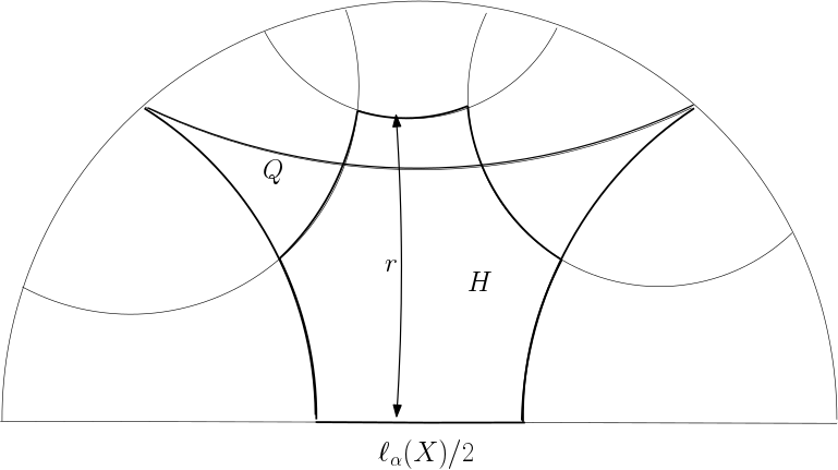
Figure 1: $r>2\sinh^{-1}(1/\sinh(\ell_{\alpha}(X)/4))$

In the usual collar lemma, the standard collars are disjoint. We emphasize that this does not hold for the collars we construct here.

Using the above we can improve our gradient bound for separating curves. We have

Theorem 5.2

Let $S$ be a finite type surface and $\ell_{\alpha}$ be a geodesic length function for $\alpha$ a simple separating curve on $S$. Then for $X\in\operatorname{Teich}(S)$

$$\|\nabla\ell_{\alpha}(X)\|^{2}\leq\frac{2\ell_{\alpha}(X)}{\pi}\left(1+F(\ell_{\alpha}(X)/2)\right).$$

Furthermore

$$d_{\rm WP}(\mathcal{S}^{a}_{\alpha},\mathcal{S}^{b}_{\alpha})\geq H_{s}(a,b)$$

where

$$H_{s}(a,b)=\int_{a}^{b}\frac{dt}{\sqrt{\frac{2t}{\pi}\left(1+F(t/2)\right)}}.$$

Proof: The proof is the same as in Theorem 1.6. The only difference is that the embedded neighborhood has width $2\sinh^{-1}(1/\sinh(\ell_{\alpha}(X)/4))$ rather than $2\sinh^{-1}(1/\sinh(\ell_{\alpha}(X)/2))$. Thus we can substitute $\ell_{\alpha}(X)/2$ into the lower bound in Corollary 2.6 to obtain the new lower bound. We note the linear factor arises from integrating in the $\alpha$ direction in the collar and therefore remains unchanged. The Weil-Petersson distance bound follows immediately as in Lemma 3.3. $\Box$

We repeat the proof of Theorem 1.2 for the punctured sphere case. For simplicity, we will let $H_{s}(t)=H_{s}(0,t)$.

Theorem 5.3

Let $\mathcal{S}_{\sigma}(S),\mathcal{S}_{\tau}(S)$ be two strata in $\operatorname{Teich}(S)$ for $S$ an $n$-punctured sphere. Then one of the following holds;

1. $i(\sigma,\tau)=0$ and $d_{\rm WP}(\mathcal{S}_{\sigma}(S),\mathcal{S}_{\tau}(S))=0.$

2. $i(\sigma,\tau)=2$ and $d_{\rm WP}(\mathcal{S}_{\sigma}(S),\mathcal{S}_{\tau}(S))=\delta_{0,4}.$

3. $i(\sigma,\tau)>2$ and $d_{\rm WP}(\mathcal{S}_{\sigma}(S),\mathcal{S}_{\tau}(S))>10.09656.$

Proof: If $i(\sigma,\tau)=0$ then the closures of the strata intersect and therefore $d_{\rm WP}(\mathcal{S}_{\sigma},\mathcal{S}_{\tau})=0$.

Now assume that $i(\sigma,\tau)=2k>0$ and that for every $\alpha\in\sigma$ we have $i(\alpha,\tau)=0$ or $2$. Then by the same argument as in Theorem 1.2 we can decompose into 4-punctured spheres and get

$$d_{WP}(\mathcal{S}_{\sigma},\mathcal{S}_{\tau})=\sqrt{k}\delta_{0,4}.$$

Therefore if $i(\sigma,\tau)=2$ we have

$$d_{\rm WP}(\mathcal{S}_{\sigma},\mathcal{S}_{\tau})=\delta_{0,4}$$

and if $i(\sigma,\tau)=2k\geq 4$ then by Lemma 2.2

$$d_{\rm WP}(\mathcal{S}_{\sigma},\mathcal{S}_{\tau})\geq\sqrt{2}\delta_{0,4}=2\delta_{1,1}>13.145.$$

Now we can assume one of the following;

• there is curve $\alpha\in\sigma$ and curve $\beta\in\tau$ with $i(\alpha,\beta)\geq 4$.

• there is curve $\alpha\in\sigma$ and curves $\beta_{1},\beta_{2}\in\tau$ and $i(\alpha,\beta_{1})=i(\alpha,\beta_{2})=2$.

In the first case, we let $c$ be any path from $\mathcal{S}_{\sigma}$ to $\mathcal{S}_{\tau}$ and choose $t_{0}$ such that at $c(t_{0})=X$ we have $\ell_{\beta}(X)=L$. Therefore by Lemma 5.1 above, $\alpha$ has an embedded collar of width $2\sinh^{-1}(1/\sinh(L/4))$. Therefore $\ell_{\alpha}(X)\geq 8\sinh^{-1}(1/\sinh(L/4))$. Then by Theorem 5.2,

$$d_{\rm WP}(\mathcal{S}_{\sigma},\mathcal{S}_{\tau})\geq H_{s}(L)+H_{s}\left(8\sinh^{-1}\left(\frac{1}{\sinh(L/4)}\right)\right)=W_{1}(L)$$

We choose $L=3.678$ and evaluating we get

$$d_{\rm WP}(\mathcal{S}_{\sigma},\mathcal{S}_{\tau})\geq W_{1}(3.678)\geq 10.76596.$$

In the second case, we choose $t_{0}$ such that at $c(t_{0})=X$ and $L=\max\{\ell_{\beta_{1}}(X),\ell_{\beta_{2}}(X)\}$. Then $\beta_{1}\cup\beta_{2}$ split $\alpha$ into 4 geodesic arcs with endpoints in $\beta_{1}\cup\beta_{2}$. Two of the arcs have endpoints in the same component of $\beta_{1}\cup\beta_{2}$ and therefore by Lemma 5.1 are both of length at least $2\sinh^{-1}(1/\sinh(L/4))$. The other two geodesic arcs have one endpoint in $\beta_{1}$ and another in $\beta_{2}$. Then using the fact that the collars about $\beta_{1},\beta_{2}$ of width $2\sinh^{-1}(1/\sinh(L/2))$ are disjoint we have each of these arcs are of length at least $2\sinh^{-1}(1/\sinh(L/2))$. Thus

$$\ell_{\alpha}(X)\geq 4\sinh^{-1}\left(\frac{1}{\sinh(L/4)}\right)+4\sinh^{-1}\left(\frac{1}{\sinh(L/2)}\right).$$

Thus

$$d_{\rm WP}(\mathcal{S}_{\sigma},\mathcal{S}_{\tau})\geq H_{s}(L)+H_{s}\left(4\sinh^{-1}\left(\frac{1}{\sinh(L/4)}\right)+4\sinh^{-1}\left(\frac{1}{\sinh(L/2)}\right)\right)=W_{2}(L).$$

We choose $L=2.420$ and get

$$d_{\rm WP}(\mathcal{S}_{\sigma},\mathcal{S}_{\tau})\geq W_{2}(2.42)\geq 10.09656.$$

Thus if $i(\sigma,\tau)>2$ then $d_{\rm WP}(\mathcal{S}_{\sigma},\mathcal{S}_{\tau})\geq 10.09656$. $\Box$

Strata distances and gaps

From the above, if $S$ has positive genus then the minimal distance between strata $\mathcal{S}_{\sigma},\mathcal{S}_{\tau}$ with $i(\sigma,\tau)\neq 0$ is $\delta_{1,1}$ and is achieved if and only if $i(\sigma,\tau)=1$. Furthermore if $i(\sigma,\tau)>1$ then the distance between the strata is at least $H(4\epsilon_{2})+H(2\epsilon_{2})$. Therefore there is a gap in the distances from $\delta_{1,1}$ to $H(4\epsilon_{2})+H(2\epsilon_{2})$ of size

$$H(4\epsilon_{2})+H(2\epsilon_{2})-\delta_{1,1}\geq 7.61138-6.65603=0.95535.$$

Similarly if $S$ is an n-punctured sphere with $n\geq 4$, then the minimal distance between strata $\mathcal{S}_{\sigma},\mathcal{S}_{\tau}$ with $i(\sigma,\tau)\neq 0$ is $\delta_{0,4}$ and is achieved if and only if $i(\sigma,\tau)=2$. Furthermore if $i(\sigma,\tau)>2$ then the distance between the strata is at least $W_{2}(2.42)$. Therefore there is a gap in the distances from $\delta_{0,4}$ to $W_{2}(2.42)$ of size

$$W_{2}(2.420)-\delta_{0,4}\geq 10.09656-9.41305=.68351.$$

6 Gradient bounds at systoles and the in-radius of $\operatorname{Teich}(S)$

A systole is a shortest closed geodesic on a Riemannian manifold. The systole function

$$\ell_{{\operatorname{sys}}}:\operatorname{Teich}(S)\rightarrow\mathbb{R}_{>0}$$

is the length of the systole at $X\in\operatorname{Teich}(S)$. The systole function is a proper, bounded function to $(0,\infty)$ (as it extends continuously to zero on $\partial\overline{{\operatorname{Teich}}(S)}$) and therefore

$${\operatorname{sys}}(S)=\max_{X\in\operatorname{Teich}(S)}\ell_{\rm sys}(X)$$

is defined. Note that for a fixed curve $\alpha$ we have bounded from below the distance between $X$ and $\mathcal{S}_{\alpha}$ in terms of $\ell_{\alpha}(X)$. One would similarly expect a lower bounded on the distance between $X$ and $\partial\overline{{\operatorname{Teich}}(S)}$ in terms of $\ell_{\operatorname{sys}}(X)$. Bounds of this type were first obtained by Wu. Before stating Wu’s result we define the in-radius of the Teichmüller space $\operatorname{Teich}(S)$ by

$$\mbox{\rm InRad}(\operatorname{Teich}(S))=\max_{X\in\mathcal{\operatorname{Teich}}(S)}d_{\rm WP}(X,\partial\overline{{\operatorname{Teich}}(S)}).$$

Then Wu proves:

Theorem 6.1 (Wu, [Wu2])

There exists a universal constant $K$ such that for all $X,Y\in\overline{{\operatorname{Teich}}(S)}$ we have

$$\left|\sqrt{\ell_{\rm sys}(X)}-\sqrt{\ell_{\rm sys}(Y)}\right|\leq Kd_{\rm WP}(X,Y).$$

Therefore

$$d_{\rm WP}(X,\partial\overline{{\operatorname{Teich}}(S)})\geq\frac{1}{K}\sqrt{\ell_{\operatorname{sys}}(X)}$$

and

$$\operatorname{InRad}(S)\geq\frac{1}{K}\sqrt{{\rm sys}(S)}.$$

By Theorem 1.5, for any length function the gradient of $\sqrt{\ell_{\alpha}}$ is uniformly bounded when the length of the curve is bounded so one would expect a similar statement to hold for $\sqrt{\ell_{\operatorname{sys}}}$ where the bound depends on ${\operatorname{sys}}(S)$. What is surprising is that there is a bound independent of topology.

Here we will show that $\sqrt{\ell_{\operatorname{sys}}}$ is $1/2$-Lipschitz and we will also give precise asymptotics for $d_{\rm WP}(X,\partial\overline{{\operatorname{Teich}}(S)})$ as $\ell_{\operatorname{sys}}(X)\to\infty$. A key observation in Wu’s work is that when a curve is a systole there are improved lower bounds on the width of embedded collars and this leads to better gradient bounds for length functions at systoles. This same observation will be central to our work.

One extra complication is that the systole function is not smooth. However it has enough regularity that we can still discuss its gradient in a modified form that will still satisfy the lower bounds from Lemma 3.1. We define

$$\|\nabla\ell_{\rm sys}(X)\|=\underset{\gamma\in{\rm sys}(X)}{\max}\|\nabla\ell_{\gamma}(X)\|$$

where ${\operatorname{sys}}(X)$ is the set of curves $\alpha$ that are systoles for $X$. Note that ${\operatorname{sys}}(X)$ is a finite set so the maximum is always defined.

Lemma 6.2

Assume that $U$ is an integrable function with

$$\|\nabla\ell_{\operatorname{sys}}(X)\|\leq U(\ell_{\operatorname{sys}}(X)).$$

Then for any $X,Y\in{\operatorname{Teich}}(S)$ we have

$$d_{\rm WP}(X,Y)\geq\left|\int_{\ell_{\operatorname{sys}}(X)}^{\ell_{\operatorname{sys}}(Y)}\frac{1}{U(s)}ds\right|.$$

Proof: Let $X_{t}$ be a smooth path from $X$ to $Y$ parameterized by $[0,1]$ and for each curve $\alpha$ let

$$f_{\alpha}(t)=\ell_{\alpha}(X_{t})\qquad\mbox{and}\qquad f_{\operatorname{sys}}(t)=\ell_{\operatorname{sys}}(X_{t}).$$

The path is a compact set in ${\operatorname{Teich}}(S)$ and as a smooth function is Lipschitz when restricted to a compact set, each $\ell_{\alpha}$ will be Lipschitz on the image and therefore each $f_{\alpha}$ will also be Lipschitz. Furthermore, on a compact set $\ell_{\operatorname{sys}}$ is the minimum of finitely many length functions so $f_{\operatorname{sys}}$ is the minimum of finitely many $f_{\alpha}$. As the minimum of finitely many Lipschitz functions is also Lipschitz we have that $f_{\operatorname{sys}}$ is Lipschitz. By standard results in analysis $f_{\operatorname{sys}}$ is differentiable almost everywhere and satisfies the fundamental theorem calculus. Also, as $f_{\operatorname{sys}}$ is the minimum of finitely many $f_{\alpha}$ whenever $f^{\prime}_{\operatorname{sys}}(t)$ exists we have

$$f^{\prime}_{\operatorname{sys}}(t)=f^{\prime}_{\alpha}(t)=d\ell_{\alpha}(\dot{X}_{t})$$

for some $\alpha\in{\operatorname{sys}}(X_{t})$. Therefore

$$|f^{\prime}_{\operatorname{sys}}(t)|\leq\|\nabla\ell_{\operatorname{sys}}(X_{t})\|\cdot\|\dot{X}_{t}\|$$

when the derivative is defined. The rest of the proof the follows exactly as in Lemma 3.1. $\Box$

While Theorem 1.6 gives bounds on $\|\nabla\ell_{\rm sys}\|$ these bounds can be significantly improved. In particular, for any closed geodesic $\gamma$ on a hyperbolic surface $X$, the collar lemma gives a uniform lower bound on $r_{\gamma}(X)$ the radius of an embedded collar about $\gamma$ depending only on $\ell_{\gamma}(X)$. If $\gamma$ is a systole then this radius is bounded below by $\ell_{\gamma}(X)/4$. For the usual collar lemma the width of the collar decreases to zero as the length grows, in contrast to here where the collar width of the systole limits to infinity. Combining this and Corollary 2.7 we can improve our upper bounds on the gradient of $\ell_{\gamma}$ at $X$. We first record the lower bound on the radius of collars of systoles in the following lemma.

Lemma 6.3

Let

$$r_{\rm sys}(t)=\max\left\{t/4,\sinh^{-1}\left(\frac{1}{\sinh(t/2)}\right)\right\}.$$

If $\gamma\in{\rm sys}(X)$ then

$$r_{\gamma}(X)\geq r_{\rm sys}(\ell_{\gamma}(X))\geq r_{\rm sys}(L_{0})$$

where $L_{0}$ is the unique positive number with $\sinh(L_{0}/4)\sinh(L_{0}/2)=1$.

Combined with Corollary 2.7 we then have:

Corollary 6.4

Let $G$ be the function from Corollary 2.7. Then

$$\|\nabla\ell_{\operatorname{sys}}(X)\|^{2}\leq\frac{2\ell_{\operatorname{sys}}(X)}{\pi}(1+G(r_{\operatorname{sys}}(X)).$$

Mimicking the definition of the function $H(a,b)$ that we used to bound from below the distance between level sets of lengths functions we define

$$\qquad H_{\rm sys}(a,b)=\int_{a}^{b}\frac{dt}{\sqrt{\frac{2t}{\pi}\left(1+G(r_{\rm sys}(t)\right)}}.$$

As before we further define $H_{\rm sys}(t)=H_{\rm sys}(0,t)$. We also let

$${\mathcal{S}}^{L}_{\operatorname{sys}}=\ell_{\operatorname{sys}}^{-1}(L)\subset\overline{{\operatorname{Teich}}(S)}$$

be the level sets of $\ell_{\operatorname{sys}}$ and note that ${\mathcal{S}}^{0}_{\operatorname{sys}}=\partial\overline{{\operatorname{Teich}}(S)}$.

Note that if $\ell_{\operatorname{sys}}(X)=b$ and $\gamma\in{\operatorname{sys}}(X)$ then by Theorem 3.3, for all $a\in[0,\infty)$ we have $d_{\rm WP}(\mathcal{S}_{\gamma}^{a},X)\leq K(a,b)$. As $\ell_{\operatorname{sys}}\leq\ell_{\gamma}$ if $a\leq b$ then, since $\ell_{\operatorname{sys}}$ is continuous, $d_{\rm WP}({\mathcal{S}}_{\operatorname{sys}}^{a},X)\leq K(a,b)$. In particular, we don’t need to modify $K(a,b)$ for the systole function and we have:

Theorem 6.5

If $0\leq a<b$ and $X\in\mathcal{S}_{\operatorname{sys}}^{b}$ then

$$H_{\operatorname{sys}}(a,b)\leq d_{\rm WP}({\mathcal{S}}_{\operatorname{sys}}^{a},{\mathcal{S}}_{\operatorname{sys}}^{b})\leq d_{\rm WP}(\mathcal{S}_{\operatorname{sys}}^{a},X)\leq K(a,b).$$

Recall that $K(a,b)=\sqrt{2\pi}\left(\sqrt{b}-\sqrt{a}\right)$. It will be useful to estimate $H_{\operatorname{sys}}(a,b)$.

Proposition 6.6

If $0\leq a<b$ then

$$H_{\operatorname{sys}}(a,b)\geq 2\left(\sqrt{b}-\sqrt{a}\right)$$

and

$$\sqrt{\frac{2}{\pi}}\leq\frac{H_{\operatorname{sys}}(t)}{\sqrt{2\pi t}}$$

with

$$\lim_{t\to 0}\frac{H_{\operatorname{sys}}(t)}{\sqrt{2\pi t}}=\lim_{t\to\infty}\frac{H_{\operatorname{sys}}(t)}{\sqrt{2\pi t}}=1.$$

Proof: We note that the $r_{\operatorname{sys}}(t)$ is the maximum of a monotonically increasing and monotonically decreasing function so it is minimized where the two functions agree. That is the minimum of $r_{\operatorname{sys}}(L_{0})=L_{0}/4$ is the minimum where $L_{0}$ is the unique positive solution to $\sinh(L_{0}/4)\sinh(L_{0}/2)=1$. Therefore

$$H_{\rm sys}(a,b)\geq\sqrt{\frac{2\pi}{1+G(L_{0}/4)}}\left(\sqrt{b}-\sqrt{a}\right).$$

To evaluate the constant term on right we need to solve $\sinh(L_{0}/4)\sinh(L_{0}/2)=1$ for $L_{0}$ and the evaluate the function $G$ at $L_{0}/4$. The function $G$ is an elementary function and can be (rigorously) evaluated using Mathematica to get

$$\sqrt{\frac{2\pi}{1+G(L_{0}/4)}}\simeq 2.00423$$

and, in particular, it is greater than two. Both inequalities then follow.

For the two limits we observe that $r_{\operatorname{sys}}(t)$ tends to infinity both as $t\to 0$ and $t\to\infty$ while

$$\lim_{t\to\infty}G(t)=0.$$

The two limits follow. $\Box$

We note that in [Wu2, Theorem 1.4] Wu obtains similar bounds to Theorem 6.5. In both Theorems the upper bound is the same and follows directly from the lower bound in Riera’s formula. In [Wu2, Theorem 1.4] the lower bound is also uniformly comparable to $\sqrt{b}-\sqrt{a}$ as in Theorem 6.5.

Remark: A more detailed analysis of the function $\frac{H_{\operatorname{sys}}(t)}{\sqrt{2\pi t}}$ shows that it has a unique critical point which is therefore a global minimum. Evaluating at this minimum gives $\frac{H_{\operatorname{sys}}(t)}{\sqrt{2\pi t}}\geq.94$ (see Figure 2).

As an immediate corollary to Theorem 6.5 we have:

Corollary 6.7

The function $\sqrt{\ell_{\operatorname{sys}}}$ is 1/2-Lipschitz.

We note that using different methods, Wu shows that $\sqrt{\ell_{\rm sys}}$ is Lipschitz with constant $.5492$ for the closed case $S_{g}$ (see [Wu1]).

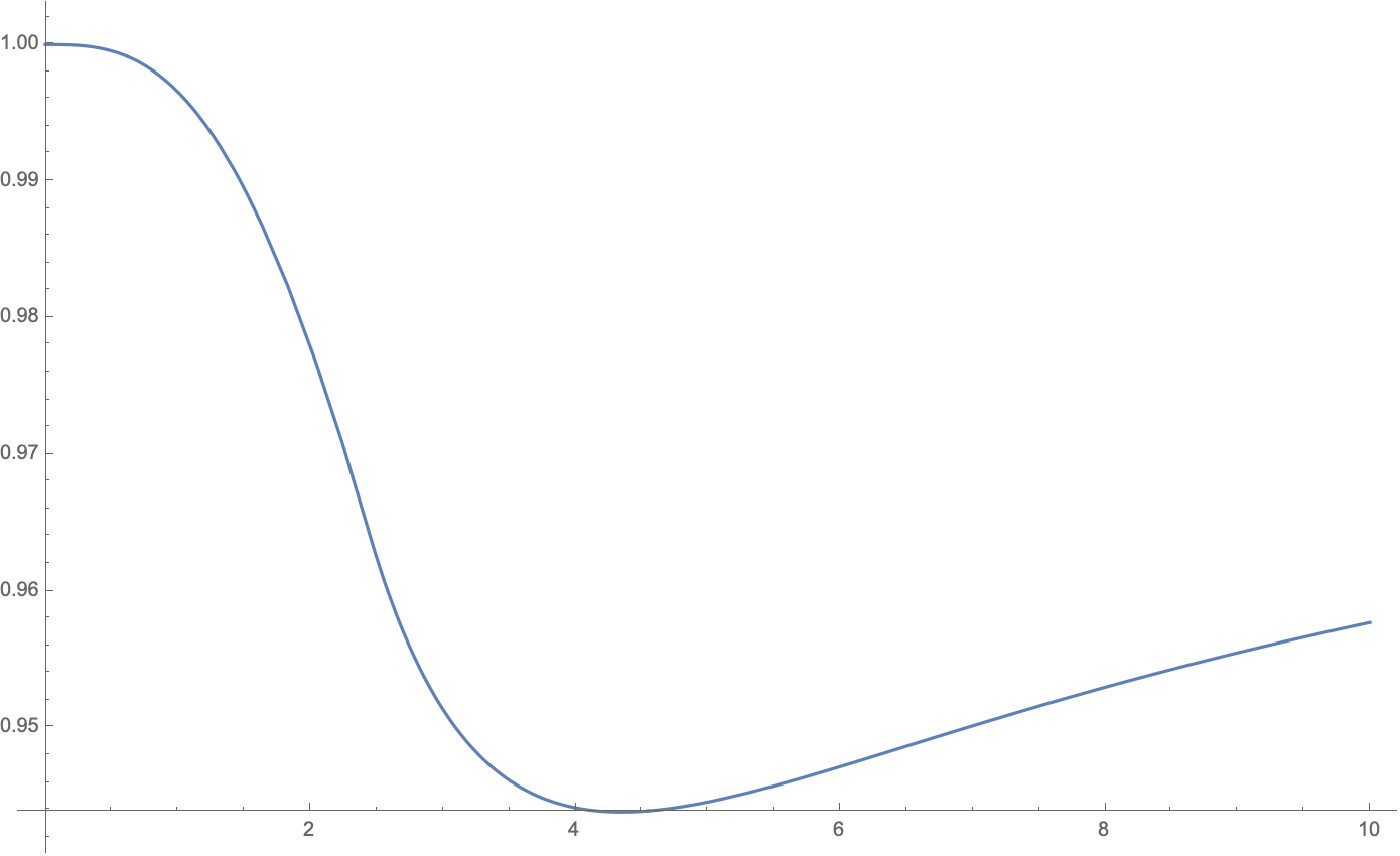
Figure 2: The graph of $\frac{H_{\operatorname{sys}}(t)}{\sqrt{2\pi t}}$

We also obtain bounds on ${\rm InRad}(S_{g,n})$. For this we apply our work here to bounds on ${\operatorname{sys}}(S_{g,n})$. For example when $n$ is fixed by [BMP] we have

$$\lim_{g\rightarrow\infty}{\rm sys}(S_{g,n})=\infty.$$

If $g$ is fixed then ${\operatorname{sys}}(S_{g,n})$ is uniformly bounded (also see [BMP]). However, it is uniformly bounded below by $2\epsilon_{2}$.

Thus we have:

Corollary 6.8

For any hyperbolic surface $S$ we have

$$\sqrt{\frac{2}{\pi}}\leq\frac{H_{\operatorname{sys}}({\operatorname{sys}}(S))}{\sqrt{2\pi{\operatorname{sys}}(S)}}\leq\frac{{\rm InRad}({\operatorname{Teich}}(S))}{\sqrt{2\pi{\operatorname{sys}}(S)}}\leq 1,$$

and therefore

$$\lim_{g\rightarrow\infty}\frac{{\rm InRad}(\operatorname{Teich}(S_{g,n}))}{\sqrt{2\pi{\rm sys}(S_{g,n})}}=1$$

and

$${\rm InRad}(\operatorname{Teich}(S_{g,n}))\geq H_{\operatorname{sys}}(2\epsilon_{2})=H(2\epsilon_{2})\simeq 3.27466.$$

We note that in [Wu2, Theorem 1.2] it was shown that ${\rm InRad}({\operatorname{Teich}}(S))$ is uniformly bounded below without producing a concrete bound. We also remark that that, as in Theorem 5.3, using the fact that we obtain improved lower bounds on the width of collar neighborhoods of separating curves one can show that

$${\rm InRad}(\operatorname{Teich}(S_{0,n}))\geq H_{s}(4\epsilon_{2})\simeq 4.63108.$$

Computation

The calculation of $H,H_{s},H_{\rm sys}$ are by numerical integration using Mathematica. The integrand in each can be written in terms of $F$ where $F(t)=a(T)u(t)v(t)$ where $T=2\sinh^{-1}(1/\sinh(t/2))$. The functions $a,u$, and $h$ are elementary functions involving trigonometric, exponential and log functions. To calculate the function $a$ for $t$ small with precision we cannot use its description in terms of basic functions and must instead use a series expansion. The reason for this is that although $a$ is monotonic and $a(0)=8/3$, the expression for $a$ for small $t$ is the difference of two large numbers with the computation being of the form $(t^{-4}+8/3\pi^{2})-t^{-4}$. To avoid this problem and have arbitrarily high precision, we use the series for the function $\hat{a}$ introduced in Lemma 2.3 and the relation

$$a(T)=\hat{a}\left(e^{-T}\right)=\hat{a}\left(\frac{\cosh(t/2)-1}{\cosh(t/2)+1}\right).$$

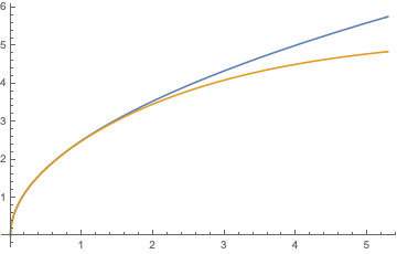
Figure 3: Graph of H versus K

See Figure 3 for a comparison of $H(t)$ and $K(t)=\sqrt{2\pi t}$.

Appendix: Closed geodesics in the moduli space of the punctured torus

Our methods can also be used to obtain lower bounds on the minimal Weil-Petersson translation length of a pseudo-Anosov mapping class acting on Teichmüller space. We demonstrate the method on the Teichmüller space of punctured tori. For a surface of higher complexity the basic idea will still work but it be harder to get explicit estimates.

Let $T$ be the punctured torus and

$$\psi\colon T\to T$$

a pseudo-Anosov mapping class. By [DW] there is a unique $\psi$-invariant geodesic $\gamma$ in the Weil-Petersson metric on $\operatorname{Teich}\left(S_{1,1}\right)$. This will descend to a closed geodesic in the moduli space $\mathcal{M}_{1,1}$. We can use our estimates to give a lower bound on the length of the shortest such geodesic.

We identify $\operatorname{Teich}(T)$ so that $\psi$ can be represented by an element of $SL_{2}(\mathbb{Z})$:

$$\psi=\left(\begin{array}[]{cc}a&b\\ c&d\end{array}\right).$$

We can conjugate $\psi$ so that the axis $\gamma$ crosses the imaginary axis at some punctured torus $X$. (This is equivalent to $b/c>0$.) Then $X$ is rectangular: the $(1,0)$-curve and $(0,1)$-curve are represented by geodesics $\alpha$ and $\beta$ that meet orthogonally at a single point. A standard calculation shows that

$$\sinh(\ell_{\alpha}(X)/2)\sinh(\ell_{\beta}(X)/2)=1.$$

One of these two curves will be the systole on $X$ (with the other the second shortest curve). In fact this is exactly the situation where the collar lemma is optimal: the width of the collar about $\alpha$ is $\ell_{\beta}(X)$ In a particular if $i(\alpha,\gamma)=k$ then

$$\ell_{\gamma}(X)\geq k\ell_{\beta}(X).$$

We have a similar statement when we switch the roles of $\alpha$ and $\beta$.

As $X$ lies on the axis $\gamma$ the translation length of $\psi$ is $d_{\rm WP}(X,\psi(X))$. To bound this distance from below we observe that for any curve $\ell_{\psi(\gamma)}(X)=\ell_{\gamma}(\psi(X))$. We assume that $\alpha$ is the shortest curve.

If $i(\alpha,\psi(\alpha))\geq 2$ then

$$\ell_{\alpha}(X)\leq 2\epsilon_{2}\mbox{ and }\ell_{\psi(\alpha)}(X)\geq 2\cdot 2\epsilon_{2}$$

so by Lemma 3.3

$$d_{\rm WP}(X,\psi(X)) \geq d_{\rm WP}(\mathcal{S}^{2\epsilon_{2}}_{\alpha},\mathcal{S}^{4\epsilon_{2}}_{\alpha})$$

$$\geq H(2\epsilon_{2},4\epsilon_{2})$$

$$\geq 1.06205$$

It follows that for $\psi$ with $i(\alpha,\psi(\alpha))\geq 2$ then

$$\|\psi\|_{\rm WP}\geq 1.06205.$$

Otherwise as $\psi(\alpha)=(a,c)$ then $|c|=1$ and $\psi^{2}(\alpha)=(a^{2}+bc,c(a+d))$. As $|a+d|>2$ then $i(\alpha,\psi^{2}(\alpha))=|c(a+d)|=|a+d|\geq 3$ and

$$\ell_{\alpha}(X)\leq 2\epsilon_{2}\mbox{ and }\ell_{\psi(\alpha)}(X)\geq 3\cdot 2\epsilon_{2}.$$

Therefore

$$d_{\rm WP}(X,\psi^{2}(X)) \geq d_{\rm WP}(\mathcal{S}^{2\epsilon_{2}}_{\alpha},\mathcal{S}^{6\epsilon_{2}}_{\alpha})$$

$$\geq H(2\epsilon_{2},6\epsilon_{2})$$

$$\geq 1.56949.$$

Therefore in general

$$\|\psi\|_{\rm WP}\geq\frac{1.56949}{2}\geq.78474.$$

In [BB], the second author and Brock give a lower bound on the systole for of $\operatorname{Teich}(S_{g,n})$ using renormalized volume and the lower bound for the volume of a hyperbolic 3-manifold. They prove

Theorem 6.9 (Brock-Bromberg, [BB])

Let $\gamma$ be a closed geodesic for the Weil-Petersson metric on moduli space $\mathcal{M}_{g,n}$ of the surface $S_{g,n}$ with $n>0$. Then

$$\ell_{\rm WP}(\gamma)\geq\frac{4\mathcal{V}_{3}}{3\sqrt{\mbox{Area}(S_{g,n})}}$$

where $\mathcal{V}_{3}$ is the volume of the regular ideal hyperbolic tetrahedron.

We note that for $\mathcal{M}_{1,1}$, the above theorem gives a bound of $.53724$ and our bound is $.78474$. While a more refined analysis could improve this bound, it seems unlikely that these estimates are close to optimal so we do not include them.

References

- [BMP] Florent Balacheff, Eran Makover, and Hugo Parlier. Systole growth for finite area hyperbolic surfaces. Annales de la faculté des sciences de Toulouse Mathématiques 23(2014), 175–180.
- [BH] M. Bridson and A. Haefliger. Metric Spaces of Non-Positive Curvature. Springer-Verlag, 1999.
- [BB] J. Brock and K. Bromberg. Inflexibility, Weil-Petersson distance, and volumes of fibered 3-manifolds. Math. Res. Lett. 23(2016), 649–674.
- [DW] Georgios Daskalopoulos and Richard Wentworth. Classification of Weil-Petersson isometries. Amer. J. Math. 125(2003), 941–975.
- [Par] Hugo Parlier. A Note on Collars of Simple Closed Geodesics. Geometriae Dedicata 112(2005), 165–168.
- [Rie] Gonzalo Riera. A formula for the Weil-Petersson product of quadratic differentials. Journal d’Analyse Mathématique 95(2005), 105–120.
- [Wol1] S. Wolpert. Geodesic length functions and the Nielsen problem. J. Diff. Geom. 25(1987), 275–296.
- [Wol2] S. Wolpert. Geometry of the Weil-Petersson completion of Teichmüller space. In Surveys in differential geometry, Vol. VIII (Boston, MA, 2002), Surv. Differ. Geom., VIII, pages 357–393. Int. Press, Somerville, MA, 2003.
- [Wol3] S. Wolpert. Behavior of geodesic-length functions on Teichmüller space. J. Differential Geom. 79(2008), 277–334.
- [Wu1] Y. Wu. A new uniform lower bound on Weil-Petersson distance. preprint 2020.
- [Wu2] Yunhui Wu. Growth of the Weil–Petersson inradius of moduli space. Annales de l’Institut Fourier 69(2019), 1309–1346.
- [Yam] Sumio Yamada. On the geometry of Weil-Petersson completion of Teichmüller spaces. Math. Res. Lett. 11(2004), 327–344.