Thermoelectric and electron heat rectification properties of quantum dot superlattice nanowire arrays

Abstract

Heat engines made of quantum-dot (QD) superlattice nanowires (SLNWs) offer promising applications in energy harvesting due to the reduction of phonon thermal conductivity. In solid state electrical generators (refrigerators), one needs to generate (remove) large amount of charge current (heat current). Consequently, a high QD SLNW density is required for realistic applications. This study theoretically investigated the properties of power factor and electron heat rectification for an SLNW array under the transition from a one dimensional system to a two dimensional system. The SLNW arrays show the functionality of heat diodes, which is mainly attributed to a transmission coefficient with a temperature-bias direction dependent characteristic.

I Introduction

The semiconductor quantum dots (QDs) resulting from the quantum confinement of heterostructures exhibit atom-like discrete electron energy levels, QDs are also called artificial atoms. Due to the localized wave functions of nanoscale QDs, electron Coulomb interactions are too strong to be ignored. The Coulomb blockade effect [Su, 1,Field, 2] and the Kondo effect [Madhavan, 3,Cron, 4] are experimentally reported to reveal how electron Coulomb interactions influence electron transport in different temperature regimes. Because the size and location of individual QDs can be precisely controlled by the modern semiconductor technique, the sophisticated QD molecule junction systems can be laid out [Deng, 5-Gustavsson, 12]. Recently, nanowires with end QDs are proposed to clarify the Majorana bound state, which is believed to be very useful in the application of quantum computing.[Deng, 5] Based on the charge filter feature of QDs, the transport behavior of single electron transistors made of QDs of different materials have been extensively studied.[Guo, 6-Kuba, 8]. In addition, single photon sources[Michler, 9-Chang, 11] and single photon detectors[Gustavsson, 12] made of QDs are proposed for the applications of quantum optics.

Apart from the above promising applications, scientists have also focused on the thermoelectric (TE) properties of QD 3-D and 2-D crystals for the applications of energy harvesting[Harman, 13,Chen, 14]. The figure of merit $ZT=2$ of QD 3-D superlattice was experimentally reported [Harman, 13]. This enhancement is due to the reduction of phonon thermal conductivity, which is mainly attributed to the increase of phonon scattering resulting from the interfaces of QDs. $ZT$ values higher than 4 and 6 are respectively predicted for 5 nm diameter $PbSe/PbS$ and $PbTe/PbSe$ of superlattice nanowires (SLNW) at $77K$ in Ref. [Lin, 15], where the free electron model is employed to illustrate the electron thermoelectric properties. Conventional thermoelectric materials employ the doping method to provide the carriers .[Chen, 14,Lin, 15] However, Mahan and Wood proposed to utilize the thermionic procedure to provide the carriers [Mahan, 16] while avoiding the electronic defects caused by ion implantation.[Rama, 17]

The phonon thermal conductivity of silicon/germanium SLNWs can be reduced one order magnitude when compared with that of silicon nanowires.[Hu, 18] This implies that the $ZT$ of SLNWs has a potential to reach high values.[Karbaschi, 19-Whitney2, 21] In solid state electrical generators (refrigerators), one needs to generate (remove) large amount of charge current (heat current). Consequently, a high SLNW density is required for realistic applications. Here, we systematically study the thermoelectric properties of SLNWs connected to electrodes in the linear and nonlinear response regimes.

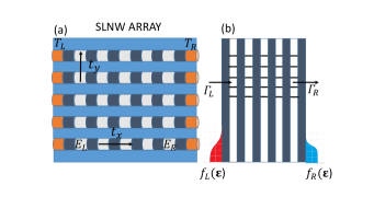
Figure 1: (a) Schematic diagram of a quantum dot superlattice nanowire (SLNW) array connected to electrodes with different equilibrium temperatures $T_{L}$ and $T_{R}$. $t_{x}$ and $t_{y}$ denote, respectively, the electron hopping strengths in the x and y directions. For simplicity, only the nearest neighbor hopping procedure is considered. (b) Band diagram of an SLNW array. $\Gamma_{L}$ and $\Gamma_{R}$ denote,respectively, the tunneling rates of electrons to tunnel from the left and right electrodes into the outer quantum dots of an SLNW array.

II Formalism

To model the thermoelectric properties of an SLNW array, the Hamiltonian of the system shown in Fig. 1 is given by $H=H_{0}+H_{QD}$,[Haug, 22] where

$$H_{0} = \sum_{k,\sigma}\epsilon_{k}a^{\dagger}_{k,\sigma}a_{k,\sigma}+\sum_{k,\sigma}\epsilon_{k}b^{\dagger}_{k,\sigma}b_{k,\sigma}$$

$$+ \sum_{\ell}^{N_{y}}\sum_{k,\sigma}V^{L}_{k,\ell,j}d^{\dagger}_{\ell,j,\sigma}a_{k,\sigma}+\sum_{\ell}^{N_{y}}\sum_{k,\sigma}V^{R}_{k,\ell,j}d^{\dagger}_{\ell,j,\sigma}b_{k,\sigma}+H.c.$$

The first two terms of Eq. (1) describe the free electron gas in the left and right electrodes. $a^{\dagger}_{k,\sigma}$ ($b^{\dagger}_{k,\sigma}$) creates an electron of momentum $k$ and spin $\sigma$ with energy $\epsilon_{k}$ in the left (right) electrode. $V^{L}_{k,\ell,j}$ ($V^{R}_{k,\ell,j}$) describes the coupling between the left (right) lead with its adjacent QD in the $\ell$th row, which counts from 1 to $N_{y}$.

$$H_{QD} = \sum_{\ell,j,\sigma}E_{\ell,j}d^{\dagger}_{\ell,j,\sigma}d_{\ell,j,\sigma}$$

$$+ \sum_{\sigma}\sum_{\ell 1,\ell 2}^{N_{y}}\sum_{j1,j2}^{N_{x}}t_{\ell 1,\ell 2,j1,j2}d^{\dagger}_{\ell 1,j1,\sigma}d_{\ell 2,j2,\sigma}+H.c,$$

$$t_{\ell 1,\ell 2,j1,j2}=\{\begin{array}[]{ll}t_{y,\ell,\ell+1}&if~{}j1=j2,|\ell 1-\ell 2|=1\\ t_{x,j,j+1}&if~{}\ell 1=\ell 2,|j1-j2|=1\end{array}.$$ (3)

where $E_{\ell,j}$ is the energy level of QD in the ${\ell}$-th row and $j$-th column. The spin-independent $t_{\ell 1,\ell 2,j1,j2}$ describes the electron hopping strength, which is limited to the nearest neighboring sites. $d^{\dagger}_{\ell 1,j1,\sigma}(d_{\ell 2,j2,\sigma})$ creates (destroys) one electron in the QD at the $\ell$th row and $j$th column. If the wavefunctions of electrons in each QD are localized, the interdot and intradot Coulomb interactions between electrons are strong. Their effects on electron transport are significant in the scenario of weak hopping strengths.[Kuo5, 23] On the other hand, the wave functions of electrons are delocalized in the scenario of strong hopping strengths, therefore their weak electron Coulomb interactions can be ignored.[Lin, 15]

To study the transport properties of an SLNW array junction connected to electrodes, it is convenient to use the Green-function technique. Using the Keldysh-Green’s function technique[Haug, 22,Meir, 24], electron and heat currents leaving electrodes can be expressed as

$$J = \frac{2e}{h}\int{d\epsilon}~{}T_{LR}(\epsilon)[f_{L}(\epsilon)-f_{R}(\epsilon)],$$ (4)

and

$$Q_{e,L(R)}$$

$$= \frac{\pm 2}{h}\int{d\epsilon}~{}T_{LR}(\epsilon)(\epsilon-\mu_{L(R)})[f_{L}(\epsilon)-f_{R}(\epsilon)]$$

where $f_{\alpha}(\epsilon)=1/\{\exp[(\epsilon-\mu_{\alpha})/k_{B}T_{\alpha}]+1\}$ denotes the Fermi distribution function for the $\alpha$-th electrode, where $\mu_{\alpha}$ and $T_{\alpha}$ are the chemical potential and the temperature of the $\alpha$ electrode. $e$, $h$, and $k_{B}$ denote the electron charge, the Planck’s constant, and the Boltzmann constant, respectively. $T_{LR}(\epsilon)$ denotes the transmission coefficient of an SLNW array connected to electrodes, which can be solved by the formula $T_{LR}(\epsilon)=4Tr[\hat{\Gamma}_{L}\hat{G}^{r}_{D,A}(\epsilon)\hat{\Gamma}_{R}\hat{G}^{a}_{D,A}(\epsilon)]$, where the matrix of tunneling rates ($\hat{\Gamma}_{L}$ and $\hat{\Gamma}_{R}$) and Green’s functions ($\hat{G}^{r}_{D,A}(\epsilon)$ and $\hat{G}^{a}_{D,A}(\epsilon)$) can be constructed as shown by the example in the appendix.[YangNX, 25]

In the linear response regime, the electrical conductance ($G_{e}$) and Seebeck coefficient ($S$) can be evaluated by using Eq. (4) with small applied bias $\Delta V=(\mu_{L}-\mu_{R})/e$ and $\Delta T=T_{L}-T_{R}$. We obtain $G_{e}=e^{2}{\cal L}_{0}$ and $S=-{\cal L}_{1}/(eT{\cal L}_{0})$. ${\cal L}_{n}$ is given by

$${\cal L}_{n}=\frac{2}{h}\int d\epsilon~{}T_{LR}(\epsilon)(\epsilon-E_{F})^{n}\frac{\partial f(\epsilon)}{\partial E_{F}},$$ (6)

where $f(\epsilon)=1/(exp^{(\epsilon-E_{F})/k_{B}T}+1)$ is the Fermi distribution function of electrodes at equilibrium temperature $T$.

III Results and discussion

III.1 A Single SLNW

Our discussion begins with a single short SLNW which can be implemented with current semiconductor fabrication techniques [Guerfi, 26]. In Fig. 2 we calculate the transmission coefficient $T_{LR}(E_{F})$ as a function of QD energy level ($\Delta=E_{0}-E_{F}$) with the homogenous electron hopping strength of $t_{x,j,j+1}=t_{c}=6\Gamma_{0}$ for an SLNW with QD number $N_{x}=N=5$ and one energy level for each QD. All energy scales are in units of $\Gamma_{0}=1~{}meV$ through out this article. Meanwhile, we have adopted symmetrical tunneling rates $\Gamma_{L}=\Gamma_{R}=\Gamma$. Diagrams (a),(b) and (c) consider different tunneling rates of $\Gamma=1\Gamma_{0},3\Gamma_{0}$ and $6\Gamma_{0}$, respectively. Fig. 2(a) clearly shows the electronic structures of a single SLNW. The resonant channels of Fig. 2(a) are given by $\epsilon=E_{0}-2t_{c}~{}cos(\frac{n\pi}{N+1})$ with $n=1,2,..N$, which is a simple tight-binding outcome with non-periodic boundary condition and ignores the effect of electrodes. Electron transport in Fig. 2(a) illustrates QD Fabry Perot type oscillations.[Whitney2, 21] When $\Gamma$ increases up to $6\Gamma_{0}$, the electronic structure of SLNW can not be resolved completely. We note that the resonant channels predicted by $\epsilon=E_{0}-2t_{c}~{}cos(\frac{n\pi}{N+1})$ are shifted in Fig. 2(c) due to the strong coupling between the outer QDs and the electrodes. The electronic structure of N-QDs shows $N-2$ resonant channels at large tunneling rates ($\Gamma=12\Gamma_{0}=2t_{c}$). Such a behavior results from that the outer QDs replace the role of electrodes when $\Gamma\geq 2t_{c}$. The results of Fig. 2 indicate that the distribution of $T_{LR}(\epsilon)$ depends on $t_{x,j,j+1}$ and $\Gamma$ values. Ref. [Whitney1, 20] pointed out that the maximum efficiency of heat engines with finite output power will be reached when the transmission coefficient maintains a square form . However, it is not yet clear how a $T_{LR}(\epsilon)$ with square form may be constructed. A single quantum dot chain has been proposed to realize the boxcar form of $T_{LR}(\epsilon)$ [Whitney2, 21], but its $G_{e}$, $S$ and power factor $PF=S^{2}G_{e}$ are lacking.

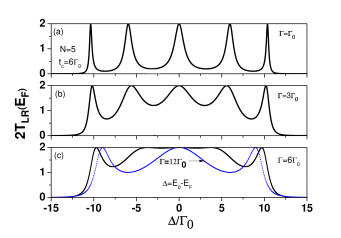
Figure 2: Transmission coefficient $T_{LR}(E_{F})$ as a function of QD energy level for $N=5$ and $t_{x,j,j+1}=t_{c}=6\Gamma_{0}$. Diagrams (a), (b) and (c) are for $\Gamma=1\Gamma_{0}$,$\Gamma=3\Gamma_{0}$ and $\Gamma=6\Gamma_{0}$ in that order. The extra curve in diagram (c) (triangles) for $\Gamma=12\Gamma_{0}$.

To examine the effect of boxcar form of $T_{LR}(\epsilon)$ on the thermoelectric properties of SLNWs,[Whitney1, 20,Whitney2, 21] we calculate $G_{e}$, $S$ and $PF$ by considering inhomogenous electron hopping strengths in Fig. 3. The electron hopping strengths $t_{12}=t_{45}=0.78\Gamma$ and $t_{23}=t_{34}=0.56\Gamma$ are adopted for $N=5$ and $\Gamma=6\Gamma_{0}$. The curve with triangle marks of $G_{e}$ (at $k_{B}T=0$) in Fig. 3(a) corresponds to the boxcar form transmission coefficient.[Whitney2, 21] The temperature-dependent $G_{e}$ shows a typical thermal broadening feature. The Seebeck coefficient is extremely small in the highly conductive region ($|\Delta|\leq 6\Gamma_{0}$). The Seebeck coefficients have different signs for positive and negative $\Delta$ values. The negative (positive) $S$ indicates that the electron transports of electrodes are mainly dominated by the resonant channels above (below) the Fermi energy of electrodes. In general, electrons of electrodes tunneling through the resonant channels below $E_{F}$ are called holes. Therefore, the change of sign in the Seebeck coefficients is called bipolar behavior.[Kuo5, 23] The peak position of $PF$ shifts away from $E_{F}$ when the temperature increases.

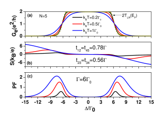
Figure 3: (a) Electrical conductance, (b) Seebeck coefficient and (c) power factor $PF$ as a function of $\Delta=E_{0}-E_{F}$ for different temperature at $N=5$, $\Gamma=6\Gamma_{0}$, $t_{12}=t_{45}=0.78\Gamma$ and $t_{23}=t_{34}=0.56\Gamma$ . The $PF$ is in the units of $k^{2}_{B}/h$. The curve with triangle marks in Fig. 3(a) corresponds to the boxcar-form transmission coefficient ($G_{e}=\frac{2e^{2}}{h}T_{LR}(E_{F})$).

Now we discuss in detail the differences of power factor between the transmission coefficients in Fig. 2 and Fig. 3. In Fig. 4 $G_{e}$, $S$ and $PF$ as a function of temperature for different $\Delta$ values at $N=5$ are calculated. Diagrams (a),(b) and (c) consider the quasi-square form $T_{LR}(\epsilon)$ given at the condition of $t_{x,j,j+1}=t_{c}$ and $t_{c}=\Gamma=6\Gamma_{0}$. In the quasi-square form, $G_{e}$ drops quickly for $\Delta=10\Gamma_{0}$ when $k_{B}T$ is below 1.5$\Gamma_{0}$. Such a behavior is attributed to the electron transport mainly resulting from resonant tunneling procedure and the electron population below $E_{F}$ is reduced with increased temperature. When $\Delta=20\Gamma_{0}$ and $\Delta=30\Gamma_{0}$ (resonant channels are far away from the $E_{F}$ of electrodes), the electron transports between the electrodes are dominated by the thermionically-assisted tunneling procedure (TATP).[Mahan, 16] For diagrams (d),(e) and (f), the curves of $G_{e}$, $S$ and $PF$ correspond to the boxcar transmission function in Fig. 3. If the curve of Fig. 4(c) at $\Delta=10\Gamma_{0}$ is compared with that of Fig. 4(f), the maximum $PF$ given by the boxcar form is larger than that of the quasi-square form. For $\Delta=10\Gamma_{0}$, the Seebeck coefficient of the boxcar form is much larger than that of the quasi-square form. For two other cases $\Delta=20\Gamma_{0}$ and $\Delta=30\Gamma_{0}$, the $PF$ of the quasi-square form is better than that of the boxcar form. As for the electron Coulomb interactions, which are important for SLNWs in the Coulomb blockade regime, we have demonstrated that $PF$ is reduced in the presence of Coulomb interactions.[Kuo5, 23]

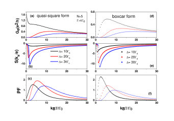
Figure 4: (a) Electrical conductance, (b) Seebeck coefficient and (c) power factor as a function of $k_{B}T$ for different $\Delta$ values at $N=5$, $t_{j,j+1}=6\Gamma_{0}$ and $\Gamma=6\Gamma_{0}$. The curves of diagrams (d), (e) and (f) consider the boxcar-form transmission coefficient in Fig. 3.

III.2 An SLNW Array

Although many studies have investigated the phonon thermal conductivity of 2-dimensional systems,[ChenG, 27-GuoYY, 30] the thermoelectric properties of an SLNW array are lacking. Fig. 5 shows the transmission coefficient $T_{LR}(E_{F})$ as a function of dot energy level $E_{\ell,j}=E_{0}=\Delta+E_{F}$ at $N_{x}=N_{y}=5$, where $N_{x}$ and $N_{y}$ are quantum dot numbers in the x and y directions, respectively. For $t_{y,\ell,\ell+1}=t_{y}=0$ and $t_{x,j,j+1}=t_{x}=6\Gamma_{0}$, $T_{LR}(E_{F})$ shows the maximum probability for the electron transport between the electrodes. The ranges of $T_{LR}(E_{F})$ are highly enhanced with increasing $t_{y}$. Fig. 5(a) illustrates the transition between a one dimensional system and a two dimensional system. The feature of $T_{LR}(\epsilon)$ involves the electronic structure of SLNW arrays given by $\epsilon=E_{0}-2t_{x}~{}cos(\frac{n_{x}\pi}{N_{x}+1})-2t_{y}~{}cos(\frac{n_{y}\pi}{N_{y}+1})$, where $n_{x}=1,2,..N_{x}$ and $n_{y}=1,2,..N_{y}$. If QDs have stronger coupling strengths in the y direction ($t_{y}>t_{x}$), how such a geometry is to influence the transport behavior of electrons. To further reveal the situation of $t_{y}>t_{x}$, we plot $T_{LR}(E_{F})$ in Fig. 5 (b) with $t_{y}=12\Gamma_{0}$ and $t_{x}=1\Gamma_{0}$. Each substructure of a main structure exhibits features similar to the structure of $t_{y}=0$ and $t_{x}=6\Gamma_{0}$ in Fig. 5(a). The behavior of Fig. 5(b) can be regarded as a single SLNW with multiple energy levels in each QD.

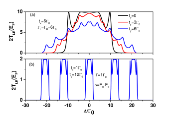
Figure 5: Transmission coefficient as a function of quantum dot energy level ($E_{\ell,j}=E_{0}-E_{F}=\Delta$) for $N_{x}=N_{y}=5$ .Diagram (a) considers $t_{x,j,j+1}=t_{x}=6\Gamma_{0}$ for different $t_{y,\ell,\ell+1}=t_{y}$ values at $\Gamma_{L}=\Gamma_{R}=6\Gamma_{0}$, and diagram (b) considers $t_{x}=1\Gamma_{0}$, $t_{y}=12\Gamma_{0}$ and $\Gamma_{L}=\Gamma_{R}=1\Gamma_{0}$.

To examine the effects of $t_{y}$ on the thermoelectric properties of an SLNW array, we calculate $G_{e}$, $S$ and $PF$ as a function of QD energy level $\Delta=E_{0}-E_{F}$ for different $t_{y}$ values at low temperature $k_{B}T=1\Gamma_{0}$ in Fig. 6. The behavior of $G_{e}$ at low temperature is significantly different from that at zero temperature ($G_{e}=\frac{2e^{2}}{h}T_{LR}(E_{F})$), however resonant tunneling procedure (RTP) still dominates the electron transport between the electrodes. $S$ is vanishingly small in highly conductive region whether the SLNW array is in the 1-D or 2-D topological structures. In addition, the maximum $S$ value of $t_{y}=0$ is the same as that of $t_{y}=6\Gamma_{0}$. In Fig. 6(c) the maximum $PF$ value is given by $PF_{1}$ for $t_{y}=0$. The results of Fig. 6 indicate that the $PF$ of the 1-D system ($t_{y}=0$) is better than that of 2-D system ($t_{y}=6\Gamma_{0}$) when the RTP dominates the electron transport.

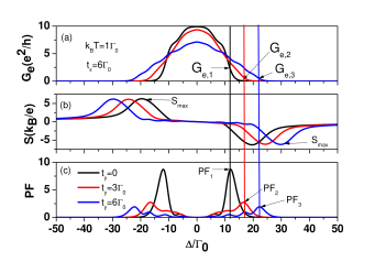
Figure 6: (a) Electrical conductance, (b) Seebeck coefficient and (c) power factor as a function of $\Delta$ for different $t_{y}$ values at $k_{B}T=1\Gamma_{0}$. Other physical parameters are the same as those of Fig. 5(a).

Because many thermoelectric devices operate at high temperatures,[Chen, 14] we examine the effects of electron hopping strengths between SLNWs on $PF$ in a large temperature range. Fig. 7 shows $S$ and $PF$ as functions of temperature for two different $t_{y}$ values. Diagrams (a) and (b) consider the case of $\Delta=10\Gamma_{0}$. Diagrams (c) and (d) consider $\Delta=30\Gamma_{0}$. The behaviors of $G_{e}$ at $t_{y}=0$ can be referred to the curves of Fig. 4(a). The trend of maximum $PF$ with respect to $t_{y}$ is the same that of $S$, because $G_{e}$ is not sensitive to $t_{y}$ at $\Delta=10\Gamma_{0}$ when $k_{B}T\geq 2.5\Gamma_{0}$. For $\Delta=10\Gamma_{0}$, we have the ratio of $PF_{1-D}/PF_{2-D}=3.9$. For $\Delta=30\Gamma_{0}$, $PF_{1-D}/PF_{2-D}$ is near one. As $\Delta$ is increased up to $\Delta=60\Gamma_{0}$, the topological effect nearly vanishes ($PF_{1-D}/PF_{2-D}=1$). This implies that the optimization of $PF$ in a 1-D system is still useful for a 2-D system as long as $\frac{t_{y}}{\Delta}\leq 0.1$.

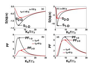
Figure 7: (a) Seebeck coefficient and (b) power factor as a function of temperature for different $t_{y}$ values at $\Delta=10~{}\Gamma_{0}$. (c) Seebeck coefficient and (d) power factor as a function of temperature for different $t_{y}$ values at $\Delta=30~{}\Gamma_{0}$. $t_{x}=6~{}\Gamma_{0}$ and $\Gamma_{L}=\Gamma_{R}=6~{}\Gamma_{0}$.

III.3 Electron Heat Rectification

Recently, many theoretical studies have devoted to the design of heat diodes (HDs).[Terraneo, 31-Craven, 36] Those designs employed three kind of heat carriers, including phonons,[Terraneo, 31-Segal, 33] photons[Otey, 34] and electrons[Kuo1, 35,Craven, 36]. So far, most experimental findings of heat rectification ratios fall between 1 and 1.4.[ChangCW, 37]Although high rectification ratio for electron HD was reported in metal/superconductor junction systems operating at extremely low temperatures (below liquid-helium temperature),[Perez, 38] it is desirable to investigate whether the SLNW arrays can show such a functionality. In Eq. (5), $Q_{e,L}+Q_{e,R}=-(\mu_{L}-\mu_{R})\times J/e$, which describes the Joule heating. To discuss the electron heat rectification, we consider the open circuit condition ($J=0$) under a temperature bias $\Delta T=T_{L}-T_{R}$, where $T_{L}=T+\Delta T/2$ and $T_{R}=T-\Delta T/2$. For $J=0$, $Q_{e,L}(\Delta T)=-Q_{e,R}(\Delta T)=Q_{e}(\Delta T)$, in which the contribution involving $\mu_{L(R)}$ is zero. Due to the Seebeck effect, the thermal voltage $V_{th}$ induced by $\Delta T$ will balance the electrons diffused from the hot electrode to the cold electrode to establish the condition of $J=0$.[Kuo1, 35,Craven, 36] Meanwhile, the energy levels $E_{\ell,j}$ will be modified due to the presence of $V_{th}$.[Craven, 36] Consequently, $T_{LR}(\epsilon)$ will depend on $V_{th}$. In addition, the Fermi distribution functions ($f_{L(R)}(\epsilon)$) also depend on the thermal voltage ($\mu_{L}=E_{F}+eV_{th}/2$ and $\mu_{R}=E_{F}-eV_{th}/2$).

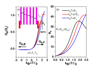
Figure 8: (a) Electron heat current and (b) heat rectification ratio as a function of temperature bias for various values of $T$ at $N_{x}=N_{y}=5$, $t_{x}=1~{}\Gamma_{0}$, $\Gamma=1~{}\Gamma_{0}$, $t_{y}=0$, $\Delta E=0.8~{}\Gamma_{0}$ and $E_{\ell,R}=E_{F}+4\Gamma_{0}$. $Q_{0}=\Gamma^{2}_{0}/h$.

We consider each SLNW with a staircase alignment of energy levels (see the inset of Fig. 8). Each QD has the position-dependent energy level only in the x-direction: $E_{\ell,j}=E_{R}+(N_{x}-j)\Delta E$, where $\Delta E$ denotes the energy level separation. Such a variation in QD levels can be engineered by considering suitable size variation of QDs in the SLNW.[Guerfi, 26] We consider an SLNW array with $N_{x}=5$ and $N_{y}=5$. Namely, we have $E_{\ell,1}=E_{R}+4\Delta E$, $E_{\ell,2}=E_{R}+3\Delta E$… and $E_{\ell,5}=E_{R}$. With an induced thermal voltage, $V_{th}$, the energy levels $E_{\ell,j}$ are modified as $\varepsilon_{\ell,j}=E_{\ell,j}+\eta_{D}eV_{th}$. In a simple approximation where the electric field is uniformly distributed in the x-direction, the level modulation factor is expressed as $\eta_{D}=-(j-3)*Ls/L$. The pair length (that of one QD plus one spacer layer) is $L_{s}$ and the length of a single SLNW is $L$. We have used their ratio $L_{s}/L=0.2$[Hu, 18]. The thermal voltage ($V_{th}$) can be evaluated by Eq. (4) under the condition of $J=0$. Once $V_{th}$ is obtained, the electron heat currents $Q_{e}(\Delta T)$ can be evaluated by Eq. (5). The resulting $Q_{e}$ as a function of temperature bias for various values of $T$ at $t_{x}=1~{}\Gamma_{0}$, $\Gamma=1\Gamma_{0}$ and $t_{y}=0$ is plotted in Fig. 8(a). In Fig. 8(a) $Q_{e}$ shows the features of thermal conductors and thermal insulators under the forward temperature bias ($\Delta T>0$) and reverse temperature bias ($\Delta T<0$), respectively. The electron heat rectification ratio of $R_{r}=\frac{Q_{e}(\Delta T>0)}{|Q_{e}(\Delta T<0)|}=\frac{Q_{e,F}}{|Q_{e,B}|}$ is plotted in Fig. 8(b). Because $Q_{e,B}$ is insensitive to the variation of $\Delta T$, the behavior of $R_{r}$ is very similar to $Q_{e,F}$. To design HDs, one needs to have a high $R_{r}$ at a small temperature bias [Chiu, 39]. Fig. 8(b) shows that $R_{r}$ is larger than ten at a small temperature bias ($\Delta T/T=0.5$).

The asymmetric behavior of $Q_{e}$ can be understood by considering $V_{th}$ as a function of $\Delta T$. $Q_{e}$ and $V_{th}$ as functions of temperature bias for different $\Delta E$ values at $k_{B}T=2\Gamma_{0}$ are plotted in Fig. 9. One see that the asymmetrical behavior of $Q_{e}$ only exists for $\Delta E\neq 0$. This implies that the staircase energy levels of SLNWs play a remarkable role in observing the electron heat rectification. Using the curve of $\Delta E=0.8\Gamma_{0}$ to illustrate the heat rectification, the QD levels are nearly aligned at $k_{B}\Delta T=1.75\Gamma_{0}$, which gives $eV_{th}=-4~{}\Gamma_{0}$, allowing the resonant tunneling of electrons from the left electrode to the right electrode. When $k_{B}\Delta T>1.75\Gamma_{0}$, $\varepsilon_{L}=E_{R}+4\Delta E+0.4eV_{th}$ and $\varepsilon_{R}=E_{R}-0.4eV_{th}$ are off-resonant, which explains why the negative differential thermal conductance (NDTC) occurs at $k_{B}\Delta T>1.75\Gamma_{0}$. Meanwhile the QD levels are misaligned under a reverse temperature bias, leading to an off-resonance condition (see insets in Fig. 9(b)).

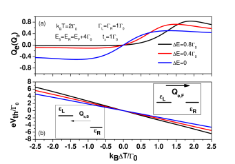
Figure 9: (a) Electron heat current and (b) thermal voltage as a function of temperature bias for various values of $\Delta E$ at $K_{B}T=2\Gamma_{0}$. Other physical parameters are the same as those of Fig. 8.

In Figures (8) and (9), we have considered the case of $t_{y}=0$. To clarify the effects of $t_{y}$ on electron heat diodes, we calculate the electron heat current and heat rectification ratio as a function of temperature bias for different $t_{y}$ values at $k_{B}T=3~{}\Gamma_{0}$ in Fig. 10. $Q_{e}$ increases with increasing $t_{y}$ values. For a finite $t_{y}$ value, the degeneracy between $E_{\ell,j}$ in y-direction is destroyed. The rectification behavior of the SLNW array can be regarded as that of a single SLNW with ”multi energy levels in each QD”. Different energy levels provide the electrons with different kinetic energies. With increasing temperature bias ($\Delta T>0$), these multi-energy levels in each QD form the multi-subbands, which substantially enhance the electron heat currents. Because of a small $\Delta E$, these multi energy levels resulting from a finite $t_{y}$ still provide some paths for electron transport in the reverse temperature bias to increase $Q_{e}$. Although the $R_{r}$ values are much reduced with increasing $t_{y}$ in Fig. 10(b), they are still very impressive when compared to some experimental findings.[ChangCW, 37]

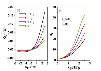
Figure 10: (a)Electron heat current and (b) heat rectification ratio, $R_{r}$ as a function of temperature bias $\Delta T$ for various values of $t_{y}$ at $k_{B}T=3\Gamma_{0}$ and $\Delta E=0.8~{}\Gamma_{0}$. Other physical parameters are the same as those of Fig. 9.Note that we use $nW$ to describe the magnitude of $Q_{e}$ instead of $Q_{0}$ for $\Gamma_{0}=1~{}meV$.

Next, we will demonstrate that the TATP also plays an important role in observing electron heat rectification. Figures 11(a) and 11(b), show $R_{r}$ and $Q_{e}$ as a function of temperature bias for different $E_{R}$ values, respectively. For $E_{R}=E_{F}$, the maximum $R_{r}$ is smaller than three. When $E_{R}$ is far away from $E_{F}$, the maximum $R_{r}$ reaches 30. Nevertheless, the magnitude of $Q_{e}$ is severely suppressed for large $E_{R}$ values. The behavior of NDTC can be observed for the cases of $\Delta_{R}=8~{}\Gamma_{0}$ and $\Delta_{R}=12~{}\Gamma_{0}$. To further clarify the results of diagram (b), we show $Q_{e}$ and the Seebeck coefficient ($S=V_{th}/\Delta T$) as functions of $E_{R}$ for different $k_{B}T$ values at $k_{B}\Delta T=2~{}\Gamma_{0}$ in diagrams (c) and (d). $Q_{e}$ decays quickly with increasing $\Delta_{R}=E_{R}-E_{F}$, whereas $V_{th}=\Delta T~{}S$ is much enhanced. When $\Delta_{R}>5\Gamma_{0}$, the TATP dominates electron transport due to all resonant channels being above $E_{F}$. The curves of $\Delta_{R}=8\Gamma_{0}$ and $\Delta_{R}=12\Gamma_{0}$ in Fig. 11(a) demonstrate that the TATP as well as $\Delta E\neq 0$ plays a critical role in observing heat rectification.

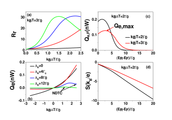
Figure 11: (a) Heat rectification ratio and (b) electron heat current as a function of temperature bias for different $\Delta_{R}=E_{R}-E_{F}$ values at $t_{x}=1\Gamma_{0}$, $t_{y}=1.5~{}\Gamma_{0}$, $\Delta E=0.8~{}\Gamma_{0}$ and $\Gamma=1~{}\Gamma_{0}$. (c) Electron heat current and (d) nonlinear Seebeck coefficient ($S=V_{th}/\Delta T$) as a function of $E_{R}$ for two different average temperatures at $k_{B}\Delta T=2~{}\Gamma_{0}$.

IV Conclusion

The thermoelectric properties of an SLNW array connected to metallic electrodes are theoretically studied by using the tight-binding Hamiltonian combined with the nonequilibrium Green’s function method. The electron current and heat current are significantly influenced by their transmission coefficients, which depend on the electron hopping strengths, QD energy levels and electron tunneling rates. These physical parameters determined by the shape and size of each QD can be calculated in the framework of effective mass theory for semiconductor QDs.[Kuo8, 40] The effects of electron interwire hopping on the optimization of power factor can be ignored if the TATP dominates the electron transport between the electrodes. In the nonlinear regime electron heat current can be highly enhanced due to proximity effect, whereas the electron heat rectification ratio is suppressed. Finally, we find that the TATP as well as staircase energy levels distributed in QDs play a very important role in observing the electron HDs with high $R_{r}$ values.

Acknowledgments
This work was supported under Contract No. MOST 107-2112-M-008 -023MY2
E-mail address: mtkuo@ee.ncu.edu.tw

V Appendix

When $N_{x}=N_{y}=2$, we have $E_{1,1}=E_{1}$, $E_{1,2}=E_{2}$, $E_{2,1}=E_{3}$ and $E_{2,2}=E_{4}$. The electron hopping strength between $E_{1(2)}$ ($E_{1(3)}$) and $E_{3(4)}$ ($E_{2(4)}$) is denoted by $t_{y}$ ($t_{x}$). The transmission coefficient $T_{LR}(\epsilon)$ of an SLNW array is calculated by the formula $T_{LR}(\epsilon)=4Tr[\hat{\Gamma}_{L}\hat{G}^{r}_{D,A}(\epsilon)\hat{\Gamma}_{R}\hat{G}^{a}_{D,A}(\epsilon)]$,[Haug, 22,YangNX, 25] where tunneling rates $\hat{\Gamma}_{L}$ and $\hat{\Gamma}_{R}$ are assumed to be energy-independent. Their forms are given by

$$\hat{\Gamma}_{L}=\Gamma_{L}\left[\begin{array}[]{cccc}1&0&0&0\\ 0&0&0&0\\ 0&0&1&0\\ 0&0&0&0\end{array}\right],$$ (7)

and

$$\hat{\Gamma}_{R}=\Gamma_{R}\left[\begin{array}[]{cccc}0&0&0&0\\ 0&1&0&0\\ 0&0&0&0\\ 0&0&0&1\end{array}\right].$$ (8)

From Eqs. (A.1) and (A.2), $E_{1}$ and $E_{3}$ ($E_{2}$ and $E_{4}$) are coupled to the left (right) electrode. $\Gamma_{L(R)}=\pi\sum_{k}|V^{L(R)}_{k,\ell,j}|^{2}\delta(\epsilon-\epsilon_{k})$. $\hat{G}^{r}_{D,A}(\epsilon)$ and $\hat{G}^{a}_{D,A}(\epsilon)$ can be calculated by their inverse matrixes ($\hat{G}^{r^{-1}}_{D,A}(\epsilon)$ and $\hat{G}^{a^{-1}}_{D,A}(\epsilon)$), which are

$$\hat{G}^{r^{-1}}_{D,A}(\epsilon)$$ (9)

$$= \left[\begin{array}[]{cccc}\epsilon-E_{1}+i\Gamma_{L}&t_{x}&t_{y}&0\\ t_{x}&\epsilon-E_{2}+i\Gamma_{R}&0&t_{y}\\ t_{y}&0&\epsilon-E_{3}+i\Gamma_{L}&t_{x}\\ 0&t_{y}&t_{x}&\epsilon-E_{4}+i\Gamma_{R}\end{array}\right],$$ (14)

and

$$\hat{G}^{a^{-1}}_{D,A}(\epsilon)$$ (15)

$$= \left[\begin{array}[]{cccc}\epsilon-E_{1}-i\Gamma_{L}&t_{x}&t_{y}&0\\ t_{x}&\epsilon-E_{2}-i\Gamma_{R}&0&t_{y}\\ t_{y}&0&\epsilon-E_{3}-i\Gamma_{L}&t_{x}\\ 0&t_{y}&t_{x}&\epsilon-E_{4}-i\Gamma_{R}\end{array}\right].$$ (20)

The imaginary parts of diagonal matrix elements result from the coupling between QDs and electrodes. Off-diagonal matrix elements ($t_{x}$ and $t_{y}$) present the electron hopping strengths between QDs. Only the nearest neighbor’s hopping strengths are included in Eqs. (A.3) and (A.4). After tedious algebra, $\hat{G}^{r}_{D,A}(\epsilon)$ is written as

$$\hat{G}^{r}_{D,A}(\epsilon)$$ (21)

$$= \frac{1}{D}\left[\begin{array}[]{cccc}a_{11}&a_{12}&a_{13}&a_{14}\\ a_{21}&a_{22}&a_{23}&a_{24}\\ a_{31}&a_{32}&a_{33}&a_{34}\\ a_{41}&a_{42}&a_{43}&a_{44}\end{array}\right],$$ (26)

where we have

$$D$$

$$= (\epsilon-E_{1}+i\Gamma_{L})(\epsilon-E_{2}+i\Gamma_{R})(\epsilon-E_{3}+i\Gamma_{L})(\epsilon-E_{4}+i\Gamma_{R})$$

$$- t^{2}_{y}(\epsilon-E_{1}+i\Gamma_{L})(\epsilon-E_{3}+i\Gamma_{L})$$

$$- t^{2}_{y}(\epsilon-E_{2}+i\Gamma_{R})(\epsilon-E_{4}+i\Gamma_{R})$$

$$- t^{2}_{x}(\epsilon-E_{1}+i\Gamma_{L})(\epsilon-E_{2}+i\Gamma_{R})$$

$$- t^{2}_{x}(\epsilon-E_{3}+i\Gamma_{L})(\epsilon-E_{4}+i\Gamma_{R})$$

$$+ (t^{2}_{x}-t^{2}_{y})^{2}$$

and

$$a_{11}$$

$$= (\epsilon-E_{2}+i\Gamma_{R})(\epsilon-E_{3}+i\Gamma_{L})(\epsilon-E_{4}+i\Gamma_{R})$$

$$- t^{2}_{y}(\epsilon-E_{3}+i\Gamma_{L})-t^{2}_{x}(\epsilon-E_{2}+i\Gamma_{R})$$

$$a_{12} = t^{3}_{x}-t^{2}_{y}t_{x}-t_{x}(\epsilon-E_{3}+i\Gamma_{L})(\epsilon-E_{4}+i\Gamma_{R})$$

$$a_{13} = t^{3}_{y}-t^{2}_{x}t_{y}-t_{y}(\epsilon-E_{2}+i\Gamma_{R})(\epsilon-E_{4}+i\Gamma_{R})$$

$$a_{14} = t_{x}t_{y}(\epsilon-E_{2}+i\Gamma_{R})+t_{x}t_{y}(\epsilon-E_{3}+i\Gamma_{L})$$

$$a_{21} = t^{3}_{x}-t^{2}_{y}t_{x}-t_{x}(\epsilon-E_{3}+i\Gamma_{L})(\epsilon-E_{4}+i\Gamma_{R})$$

$$a_{22} = (\epsilon-E_{1}+i\Gamma_{L})(\epsilon-E_{3}+i\Gamma_{L})(\epsilon-E_{4}+i\Gamma_{R})$$

$$- t^{2}_{x}(\epsilon-E_{1}+i\Gamma_{L})-t^{2}_{y}(\epsilon-E_{4}+i\Gamma_{R})$$

$$a_{23} = t_{y}t_{x}(\epsilon-E_{1}+i\Gamma_{L})+t_{y}t_{x}(\epsilon-E_{4}+i\Gamma_{R})$$

$$a_{24} = t^{3}_{y}-t^{2}_{x}t_{y}-t_{x}(\epsilon-E_{1}+i\Gamma_{L})(\epsilon-E_{3}+i\Gamma_{L})$$

$$a_{31} = t^{3}_{y}-t^{2}_{x}t_{y}-t_{y}(\epsilon-E_{2}+i\Gamma_{R})(\epsilon-E_{4}+i\Gamma_{R})$$

$$a_{32} = t_{y}t_{x}(\epsilon-E_{1}+i\Gamma_{L})+t_{y}t_{x}(\epsilon-E_{4}+i\Gamma_{R})$$

$$a_{33} = (\epsilon-E_{1}+i\Gamma_{L})(\epsilon-E_{2}+i\Gamma_{R})(\epsilon-E_{4}+i\Gamma_{R})$$

$$- t^{2}_{y}(\epsilon-E_{1}+i\Gamma_{L})-t^{2}_{x}(\epsilon-E_{4}+i\Gamma_{R})$$

$$a_{34} = t^{3}_{x}-t^{2}_{y}t_{x}-t_{x}(\epsilon-E_{1}+i\Gamma_{L})(\epsilon-E_{2}+i\Gamma_{R})$$

$$a_{41} = t_{x}t_{y}(\epsilon-E_{2}+i\Gamma_{R})+t_{x}t_{y}((\epsilon-E_{3}+i\Gamma_{L})$$

$$a_{42} = t^{3}_{y}-t^{2}_{x}t_{y}-t_{x}(\epsilon-E_{1}+i\Gamma_{L})(\epsilon-E_{3}+i\Gamma_{L})$$

$$a_{43} = t^{3}_{x}-t^{2}_{y}t_{x}-t_{x}(\epsilon-E_{1}+i\Gamma_{L})(\epsilon-E_{2}+i\Gamma_{R})$$

$$a_{44} = (\epsilon-E_{1}+i\Gamma_{L})(\epsilon-E_{2}+i\Gamma_{R})(\epsilon-E_{3}+i\Gamma_{L})$$

$$- t^{2}_{y}(\epsilon-E_{2}+i\Gamma_{R})-t^{2}_{x}(\epsilon-E_{3}+i\Gamma_{L}).$$

Although there are $16$ matrix elements, many off-diagonal matrix elements are the same. Likewise, we can obtain $\hat{G}^{a}_{D,A}(\epsilon)$. Using Eqs. (A.1), (A.2) and (A.5), the closed form of $T_{RL}(\epsilon)$ is obtained by some algebraic maneuvers. We have

$$T_{LR}(\epsilon)=\frac{c_{12}+c_{14}+c_{34}+c_{32}}{|D|^{2}}$$ (29)

where

$$c_{12}$$

$$= 4\Gamma_{L}t^{2}_{x}\Gamma_{R}|t^{2}_{x}-t^{2}_{y}-(\epsilon-E_{3}+i\Gamma_{L})(\epsilon-E_{4}+i\Gamma_{R})|^{2}$$

$$c_{14} = 4\Gamma_{L}t^{2}_{x}t^{2}_{y}\Gamma_{R}|(\epsilon-E_{2}+i\Gamma_{R})+(\epsilon-E_{3}+i\Gamma_{L})|^{2}$$

$$c_{34} = 4\Gamma_{L}t^{2}_{x}\Gamma_{R}|t^{2}_{x}-t^{2}_{y}-(\epsilon-E_{1}+i\Gamma_{L})(\epsilon-E_{2}+i\Gamma_{R})|^{2}$$

$$c_{32} = 4\Gamma_{L}t^{2}_{x}t^{2}_{y}\Gamma_{R}|(\epsilon-E_{1}+i\Gamma_{L})+(\epsilon-E_{4}+i\Gamma_{R})|^{2}$$

.

For $t_{y}=0$, $T_{LR}(\epsilon)$ is given by the simple expression below

$$T_{LR}(\epsilon)$$

$$= 4(\frac{\Gamma_{L}t^{2}_{x}\Gamma_{R}}{|(\epsilon-E_{1}+i\Gamma_{L})(\epsilon-E_{2}+i\Gamma_{R})-t^{2}_{x}|^{2}}$$

$$+ \frac{\Gamma_{L}t^{2}_{x}\Gamma_{R}}{|(\epsilon-E_{3}+i\Gamma_{L})(\epsilon-E_{4}+i\Gamma_{R})-t^{2}_{x}|^{2}}).$$

Eq. (A.10) illustrates the $T_{LR}(\epsilon)$ of two parallel serially coupled quantum dots in the absence of $t_{y}$. For $N_{x}=N_{y}=N>2$, $\hat{\Gamma}_{L}$, $\hat{\Gamma}_{R}$, $\hat{G}^{r}_{D,A}(\epsilon)$ and $\hat{G}^{a}_{D,A}(\epsilon)$ are constructed by coding to numerically calculate $T_{LR}(\epsilon)$.

References

• (1) B. Su, V. J. Goldman, and J. E. Cunningham, Science, 255, 313 (1992).
• (2) M. Field, C. G. Smith,M. Pepper, D. A. Ritchie, J. E. F. Frost, G. A. C. Jones, and D. G. Hasko, Phys. Rev. Lett. 70, 1311 (1993).
• (3) V. Madhavan, W. Chen, T. Jamneala,M. F. Crommie, and N. S. Wingreen, 280, 567 (1998).
• (4) S. M. Cronenwett, T. H. Oosterkamp, and L. P. Kouwenhoven, Science, 281, 540 (1998).
• (5) M. T. Deng,S. Vaitiekenas, E. B. Hansen,J. Danon, M. Leijnse,K. Flensberg,J. Nygard, P. Krogstrup, and C. M. Marcus, Science 354, 1557 (2016).
• (6) L. J. Guo, E. Leobandung, and S. Y. Chou, Science 275, 249 (1997).
• (7) H. W. C Postma, T. Teepen, Z. Yao, M. Grifoni, and C. Dekker, Science 293, 76 (2001).
• (8) S. Kubatkin, A. Danilov, M. Hjort, J. Cornil, J. L. Bredas, N. Stuhr-Hansen, P. Hedegard, and T. Bjornholm, Nature 425, 698 (2003).
• (9) P. Michler, A. Imamoglu, M. D. Mason, P. J. Carson, G. F. Strouse, and S. K. Buratto, Nature 406, 968 (2000).
• (10) C. Santori, D. Fattal, J. Vuckovic, G. S. Solomon, and Y. Yamamoto, Nature 419, 549 (2002).
• (11) W. H. Chang, W. Y. Chen, H. S. Chang, T. P. Hsieh, J. I. Chyi, and T. M. Hsu, Phys. Rev. Lett. 96, 117401 (2006).
• (12) S. Gustavsson, M. Studer, R. Leturcq, T. Ihn, K. Ensslin, D. C. Driscoll and A. C. Gossard, Phys. Rev. Lett. 99, 206804 (2007).
• (13) T. C. Harman, P. J. Taylor, M. P. Walsh, and B. E. LaForge, Science 297, 2229 (2002).
• (14) G. Chen, M. S. Dresselhaus, G. Dresselhaus, J. P. Fleurial, and T. Caillat, International Materials Reviews, 48, 45 (2003).
• (15) Y. M. Lin and M. S. Dresselhaus, Phys. Rev. B 68, 075304 (2003).
• (16) G. D. Mahan, L. M. Woods, Phys. Rev. Lett. 80, 4016 (1998).
• (17) E. B. Ramayya, L. N. Maurer, A. H. Davoody, I. Knezevic, Phy. Rev. B 86, 115328 (2012).
• (18) M. Hu and D. Poulikakos, Nano. Lett. 12, 5487 (2012).
• (19) H. Karbaschi, J. Loven, K. Courteaut,A. Wacker, and M. Leijnse, Phys. Rev. B, 94, 115414 (2016).
• (20) R. S. Whitney, Phys. Rev. Lett. 112, 130601 (2014).
• (21) R. S. Whitney, Phys. Rev. B 91, 115425 (2015).
• (22) H. Haug and A. P. Jauho, Quantum Kinetics in Transport and Optics of Semiconductors (Springer, Heidelberg, 1996).
• (23) D. M. T. Kuo, C. C. Chen and Y. C. Chang, Phys. Rev. B 95, 075432 (2017).
• (24) Y. Meir and N. S. Wingreen, Phys. Rev. Lett. 68, 2512 (1992).
• (25) N. X. Yang, Y. F. Zhou, P. Lv and Q. F. Sun, Phys. Rev. 97, 235435 (2018).
• (26) Y. Guerfi and G. Larrieu, Nanoscale Research Letters 11, 210 (2016).
• (27) G. Chen, Phys. Rev. B 57, 14958 (1998).
• (28) R. G. Yang, and G. Chen, Phys. Rev. B 69, 195316 (2004).
• (29) X. K. Gu, and R. G. Yang, J. Appl. Phys. 117, 025102 (2015).
• (30) Y. Y. Guo, and M. Wang, Phys. Rev. B 96, 134312 (2017).
• (31) M. Terraneo, M. Peyrard, and G. Casati, Phys. Rev. Lett. 88, 094302 (2002).
• (32) B. W. Li, L. Wang, and G. Casati, Phys. Rev. Lett. 93, 184301 (2004).
• (33) D. Segal and A. Nitzan, Phys. Rev. Lett. 94, 034301 (2005).
• (34) C. R. Otey, W. T. Lau, and S. H. Fan, Phys. Rev. Lett. 104, 154301 (2010).
• (35) David. M.-T. Kuo and Y. C. Chang, Phys. Rev. B 81, 205321 (2010).
• (36) G. T. Craven, D. H. He, A. Nitzan, Phys. Rev. Lett. 121, 247704 (2018).
• (37) C. W. Chang, D. Okawa, A. Majumdar, and A. Zettl, Science 314, 1121 (2006).
• (38) M. J. Martinez-Perez, A. Fornieri, and F. Giazotto, Nature Nanotech. 10, 303 (2015).
• (39) C. L. Chiu, C. H. Wu, B. W. Huang, C. Y. Chien, and C. W. Chang, AIP Advances 6, 121901 (2016).
• (40) David. M.-T. Kuo and Y. C. Chang, Phys. Rev. B 89, 115416 (2005).