Learning and Testing Variable Partitions

Abstract

Let $F$ be a multivariate function from a product set $\Sigma^{n}$ to an Abelian group $G$. A $k$-partition of $F$ with cost $\delta$ is a partition of the set of variables $\bm{V}$ into $k$ non-empty subsets $(\bm{X}_{1},\dots,\bm{X}_{k})$ such that $F(\bm{V})$ is $\delta$-close to $F_{1}(\bm{X}_{1})+\dots+F_{k}(\bm{X}_{k})$ for some $F_{1},\dots,F_{k}$ with respect to a given error metric. We study algorithms for agnostically learning $k$ partitions and testing $k$-partitionability over various groups and error metrics given query access to $F$. In particular we show that

1. Given a function that has a $k$-partition of cost $\delta$, a partition of cost $\mathcal{O}(kn^{2})(\delta+\varepsilon)$ can be learned in time $\tilde{\mathcal{O}}(n^{2}\operatorname{\mathrm{poly}}(1/\varepsilon))$ for any $\varepsilon>0$. In contrast, for $k=2$ and $n=3$ learning a partition of cost $\delta+\varepsilon$ is NP-hard.

2. When $F$ is real-valued and the error metric is the 2-norm, a 2-partition of cost $\sqrt{\delta^{2}+\varepsilon}$ can be learned in time $\tilde{\mathcal{O}}(n^{5}/\varepsilon^{2})$.

3. When $F$ is $\mathbb{Z}_{q}$-valued and the error metric is Hamming weight, $k$-partitionability is testable with one-sided error and $\mathcal{O}(kn^{3}/\varepsilon)$ non-adaptive queries. We also show that even two-sided testers require $\Omega(n)$ queries when $k=2$.

This work was motivated by reinforcement learning control tasks in which the set of control variables can be partitioned. The partitioning reduces the task into multiple lower-dimensional ones that are relatively easier to learn. Our second algorithm empirically increases the scores attained over previous heuristic partitioning methods applied in this context.

1 Introduction

Divide-and-conquer methods rely on the ability to identify independent sub-instances of a given instance, such as connected components of graphs and hypergraphs. When these are not available one looks for partitions into loosely related parts like small or sparse cuts. These classic problems and their variants remain at the forefront of algorithmic research [KSL15, KT15, CL15, Man17, CXY18, RSW18].

We study the related problem of function decomposition: Given a multivariate function $F(\bm{V})$ over $n$ variables $\bm{V}=\{\bm{x}_{1},\dots,\bm{x}_{n}\}$, we seek to partition the variables into $k$ groups $\bm{X}_{1},\dots,\bm{X}_{k}$ so that $F$ decomposes into a sum $F_{1}(\bm{X}_{1})+\cdots+F_{k}(\bm{X}_{k})$. In case an exact decomposition of this type is unavailable, we seek an approximate one under a suitable error metric. This algebraic partitioning question can be sensibly asked for any Abelian group. While some of our results are quite general, two particular cases of interest are addition over $\mathbb{Z}_{2}$ with respect to the Hamming metric and addition over reals with respect to the $2$-norm.

As a multivariate function is an exponentially large object, it is sensible to model the input $F$ to the partitioning problem as an oracle and allow query access to it. This departs from the common setup in (hyper)graph partitioning problems, where an explicit representation of the input is assumed to be available. While variable partitioning of real-valued functions under the 2-norm turns out to be closely related to hypergraph partitioning, the difference in input access models renders certain techniques developed for the latter (e.g., random contractions) inapplicable to our setting.

Our work is motivated by learning control variables in high-dimensional reinforcement learning control [SB18, MBM⁺16, SMSM00]. If the advantage function of the control variables can be partitioned into multiple lower-dimensional subsets, then these subsets of variables can be learned independently with a relatively easier Monte-Carlo sampling. This advantage function involves the estimates of a dynamic system, which is complex enough to not have an explicit representation available. The function is thus treated as an oracle as is in our access model. Sometimes it is natural to assume that the function should be almost decomposable; for example, if we seek to control two robots jointly performing a task, the variables controlling the respective robots are almost independent. (The robots may be collaborating so the decomposition might not be perfect.) In general, the dependencies are not known in advance but need to be learned from observed behavior. Some heuristic methods have been applied to control variable partitioning [WRD⁺18, LW18] but not rigorously analyzed.

Our contributions

Our main results are algorithmic: We show that variable partitions can be learned agnostically.

Let $F(\bm{V})$ be a function from some product set to an Abelian group $G$. A direct sum decomposition of $F$ is a partition $(\bm{X}_{1},\dots,\bm{X}_{k})$ of the set of variables $\bm{V}$ such that $F(\bm{V})$ is $F_{1}(\bm{X}_{1})+\cdots+F_{k}(\bm{X}_{k})$ for some functions $F_{1},\dots,F_{k}$. When the decomposition is imperfect, the decomposition error is measured by

$$\delta(\bm{X}_{1},\dots,\bm{X}_{k})=\min_{F_{1},\dots,F_{k}}\|F(X_{1},\dots,X_{k})-F_{1}(X_{1})-\dots-F_{k}(X_{k})\|,$$ (1)

where $\|\cdot\|\colon G\to\mathbb{R}^{+}$ is a partial norm. The definition is given in Section 2; the main examples of interest are $G=\mathbb{Z}_{q}$ under the Hamming metric $\|F\|=\operatorname{\mathrm{Pr}}[F(V)=0]$ and $G=\mathbb{R}$ under the $p$-norm $\|F\|_{p}=\mathbb{E}\bigl{[}\lvert F(V)\rvert^{p}\bigr{]}^{1/p}$ for any $p\geq 1$ under some product measure. We seek an approximation of the best-possible partition, which minimizes the objective

$$\delta_{2}(F)=\min_{\bm{X}}\delta(\bm{X},\overline{\bm{X}}),$$ (2)

for bipartition and

$$\delta_{k}(F)=\min_{\bm{X}_{1},\dots,\bm{X}_{k}}\delta(\bm{X}_{1},\dots,\bm{X}_{k}).$$ (3)

for $k$-partition. (For $p$-norms over $\mathbb{R}$ we use the notations $\|\cdot\|_{\mathbb{R},p}$, $\delta_{\mathbb{R},2}(F)$, and $\delta_{\mathbb{R},k}(F)$.)

Theorem 1.

Let $\|\cdot\|$ be either 1) $\|\cdot\|_{\mathbb{R},p}$ assuming $\|F\|_{\mathbb{R},2p}=\mathcal{O}(1)$, or 2) the Hamming metric over $\mathbb{Z}_{q}$. There is an algorithm that given parameters $n$, $k$, $\varepsilon$, $\gamma$, and oracle access to $F\colon\Sigma^{n}\to G$ outputs a $k$-partition $\mathcal{P}$ such that $\delta(\mathcal{P})\leq\mathcal{O}(kn^{2})(\delta_{k}(F)+\varepsilon)$ with probability at least $1-\gamma$. The algorithm makes $\mathcal{O}(K^{p}n^{2}\log(n/\gamma)/\varepsilon^{2p})$ queries to $F$ and runs in time linear in the number of queries, for an absolute constant $K$.

This algorithm is closely related to the heuristic ones used in the aforementioned empirical studies. However, it only guarantees optimality up to an $\mathcal{O}(kn^{2})$ approximation factor. While we do not know if an approximation factor of this magnitude is inevitable, in Proposition 17 we show that obtaining a solution with additive error is NP-hard. The proofs are given in Section 4.

In contrast, our second algorithm obtains an additive error for bipartitions of real-valued functions under the 2-norm:

Theorem 2.

Let $F\colon\Sigma^{n}\to\mathbb{R}$ be a function with $\|F\|_{\mathbb{R},4}\leq 1$. There is an algorithm that given inputs $n$, $\varepsilon$, $\gamma$, and oracle access to $F$, runs in time $\mathcal{O}(n^{5}\log(n/\gamma)/\varepsilon^{2})$ and outputs a bipartition $(\bm{X},\overline{\bm{X}})$ such that $\delta_{\mathbb{R},2}(\bm{X},\overline{\bm{X}})^{2}\leq\delta_{\mathbb{R},2}(F)^{2}+\varepsilon$ with probability at least $1-\gamma$.

More generally, we show that it is possible to output a $\sqrt{2-2/k}$-approximate $k$-partition in time $\operatorname{\mathrm{poly}}(n^{k},k,1/\varepsilon)$ (Corollary 21). For unbounded $k$ finding a good approximation is ETH hard (Corollary 19).

Theorem 2 and Corollary 19 are based on an equivalence between variable partitioning under the 2-norm and hypergraph partitioning given in Proposition 18. The results are described and proved in Section 5.

As a consequence of Theorem 1, the property of being close to a $k$-partition is testable with $\tilde{\mathcal{O}}(k^{2p}n^{4p+2}/\varepsilon^{2p})$ queries. The query complexity of the tester can be somewhat improved:

Theorem 3.

$k$-partitionability is testable with one-sided error and $\mathcal{O}(kn^{3}/\varepsilon)$ non-adaptive queries with respect to Hamming weight over $\mathbb{Z}_{q}$, and with $\mathcal{O}(k^{2p}n^{3}/\varepsilon^{2p})$ non-adaptive queries with respect to the $p$-norm over $\mathbb{R}$ assuming $\|F\|_{2p}\leq 1$.

In Section 6 we prove Theorem 3 and show that $\Omega(n-k)$ queries are necessary even for two-sided error testers.

Notation	Meaning	Notation	Meaning
$\bm{x},\bm{y}\in\bm{V}$	variables	$\delta_{k}(F)$	optimal $k$-partition error
$\bm{X},\bm{Y},\bm{\overline{X}}\subseteq\bm{V}$	sets of variables	$D_{F}(\bm{X},\bm{Y})$	dependence score
$x,y,X,Y$	(random) assignments	$\|\cdot\|,\|\cdot\|_{\mathbb{R},p}$	partial norm and $p$-norm

Ideas and techniques

Our Theorem 1 is inspired by algebraic property testing techniques. The starting point is the dual characterization of partitionability into sets $(\bm{X},\overline{\bm{X}})$ by the constraints $D_{F}(\bm{X},\bm{Y})=0$, where $D_{F}=F(X,Y)-F(X^{\prime},Y)-F(X,Y^{\prime})+F(X^{\prime},Y^{\prime})$, for all assignments $X,X^{\prime}$ to $\bm{X}$ and $Y,Y^{\prime}$ to $\bm{Y}$. David et al. [DDG⁺17] apply this relation to random inputs towards testing whether a $\mathbb{Z}_{2}$-valued function $F$ tensors decomposes into a direct sum. The acceptance probability of this test approximates the best decomposition to within a factor of 4 (Proposition 4).

Our partitioning algorithm estimates the dependence score $\|D_{F}(\bm{x},\bm{y})\|$ on every pair of variables $\bm{x},\bm{y}$ (keeping the rest fixed) to decide whether they should be partitioned or not. Here, $\|D_{F}\|$ is the probability that the test $D_{F}=0$ fails for discrete groups like $\mathbb{Z}_{2}$. In general, it can represent any error metric satisfying the axioms in Section 2. The proof of Theorem 1 amounts to showing that a collection of single variable partitions $(\bm{x},\bm{y})\in\mathcal{P}$ for which the local scores $\|D_{F}(\bm{x},\bm{y})\|$ are small can be glued together into a single $k$-partition $\mathcal{P}$ with a small global score.

When $F$ is real-valued and error is measured under the 2-norm, variable partitioning has a natural geometric interpretation. Functions that depend on different coordinates are orthogonal modulo their constant term, so the optimal decomposition with respect to a fixed partition $(\bm{X}_{1},\dots,\bm{X}_{k})$ is given by the projection of $F$ onto the respective subspaces of functions. This yields an equality between the distance and the dependence score (6) for bipartitions and a generalization to $k$-partitions (Proposition 8). Variable partitioning for functions is then equivalent to hypergraph partitioning of their orthogonal decompositions (Proposition 18), with the cost of cut $(\bm{X},\overline{\bm{X}})$ given by $\tfrac{1}{4}\|D_{F}(\bm{x},\bm{y})\|^{2}$.

This connection suggests the application of hypergraph partitioning algorithms that can be implemented with access to an approximate cut oracle, leading to Theorem 2. On the negative side it reveals that approximately optimal partitions into a large number of components are hard to find (Corollary 19).

Application to reinforcement learning control

We plug our partitioning algorithm back to reinforcement learning control. In this setting, the oracle is real-valued and as we adapt the 2-norm we use the submodularity cut algorithm described in Theorem 2.

We compare empirically with three previous approaches: The baseline that does not involve partitioning [MBM⁺16, Wil92]; the baseline that trivially partitions $n$ variables into $n$ subsets [WRD⁺18, Kos18]; the work that partitions the variables heuristically [LW18]. The way [LW18] partitions the variables is to calculate the discrete estimate of the Hessian of the oracle. Then they remove from Hessian the elements with lowest absolute values, until it forms at least $k$ connected components if the Hessian matrix is treated as the adjacency matrix.

The scores we attained on the tasks in the physics simulator are improved over these approaches, which is demonstrated in Section 7.

Relation to other learning and testing problems

A $j$-junta is a function that depends on at most $j$ of its $n$ variables. The problems of learning and testing juntas have been extensively studied [MOOS03, FKR⁺04, CG04, Bla09, Sag18, CST⁺18, Bsh19]. While a $j$-junta is always $(n-j+1)$-partitionable, the two problems are technically incomparable. Moreover, juntas are usually studied in the regime where the junta size $j$ is significantly smaller than the number of variables $n$ and are therefore partitionable into many (mostly trivial) components. In this work we are mostly interested in partitions into two or a small number of components. Nevertheless, this connection between juntas and partitionable functions is used to prove the testing lower bound in Section 6.

Dinur and Golubev [DG19] showed that the existence of decomposition with respect to a fixed $k$-partition (given as input) is testable with four queries and soundness error $\Omega(\delta)$. The case $k=2$ was already analyzed by David et al. [DDG⁺17] (see Section 3).

2 Some additional definitions

Let $F(\bm{V})$ be a function from some product set to an Abelian group $G$. In general we will assume that the variables $\bm{V}$ take values in some set $\Sigma$ endowed with a product measure which is efficiently sampleable. The quality of the partition $(\bm{X}_{1},\dots,\bm{X}_{k})$ of $\bm{V}$ is measured by $\delta(\bm{X}_{1},\dots,\bm{X}_{k})$ given in (1), where $\|\cdot\|\colon G\to\mathbb{R}^{+}$ can be any functional satisfying the following three axioms:

1. $\|0\|=0$;

2. $\|F_{1}+F_{2}\|\leq\|F_{1}\|+\|F_{2}\|$;

3. $\mathbb{E}[\|F(X,\cdot)\|\mid X]\leq\|F\|$ for any set of variables $X$ of $F$.

Our goal is to approximately optimize $\delta_{2}(F)$ in (2) and $\delta_{k}(F)$ in (3).

Our algorithms are based on the following dependence estimator inspired by the rank-1 test of [DDG⁺17]. Let $\bm{X}$ and $\bm{Y}$ be two disjoint sets of variables. The dependence estimator $D_{F}(\bm{X},\bm{Y})$ is the random variable

$$D_{F} =F(X,Y,Z)+F(X^{\prime},Y^{\prime},Z)-F(X^{\prime},Y,Z)-F(X,Y^{\prime},Z),$$

where $X,X^{\prime}$ are independent samples of the $\bm{X}$ variable, $Y,Y^{\prime}$ are independent samples of the $\bm{Y}$ variable, and $Z$ is a random sample of the remaining variables. If $F$ decomposes into a direct sum that partitions the $\bm{X}$ and $\bm{Y}$ variables then $D_{F}$ equals zero. Conversely, $\|D_{F}\|$ measures the quality of the approximation.

In the analysis it will be convenient to use the notation $F\approx_{\delta}G$ for $\|F-G\|_{p}\leq\delta$. The following two facts are immediate consequences of axioms 2 and 3:

Triangle inequality: If $F\approx_{\delta}G$ and $G\approx_{\delta^{\prime}}H$ then $F\approx_{\delta+\delta^{\prime}}H$.

Fixing: If $F(X,Z)\approx_{\delta}G(X,Z)$ then $F(\underline{X},Z)\approx_{\delta}G(\underline{X},Z)$ for some fixed value $\underline{X}$.

3 Estimating the quality of a partition

In this section we show that $\|D_{F}(\bm{X},\bm{Y})\|$ is an approximate estimator for the quality $\delta(\bm{X},\bm{Y})$ of a decomposition, namely

$$\delta(\bm{X},\bm{Y})\leq\|D_{F}(\bm{X},\bm{Y})\|\leq 4\cdot\delta(\bm{X},\bm{Y}).$$ (4)

The proof is given in Claims 5 and 6 below. As $\|D_{F}(\bm{X},\bm{Y})\|$ can be estimated efficiently from oracle access to $F$ (Claim 7), we obtain an algorithm for estimating the quality of a partition to within a factor of 4 in general, and exactly for the 2-norm over $\mathbb{R}$.

Proposition 4.

Let $\|\cdot\|$ be either 1) $\|\cdot\|_{\mathbb{R},p}$ assuming $\|F\|_{\mathbb{R},2p}=\mathcal{O}(1)$, or 2) the Hamming metric over $\mathbb{Z}_{q}$. There is an algorithm that given a bipartition $\bm{X},\bm{Y}$ of the variables and parameters $\varepsilon,\gamma>0$, outputs a value $\hat{\delta}$ such that

$$\delta(\bm{X},\bm{Y})\leq\hat{\delta}\leq 4\cdot\delta(\bm{X},\bm{Y})+\varepsilon,$$

with probability at least $1-\gamma$ from $K^{p}{\log(1/\gamma)}/{\epsilon^{2p}}$ queries to $F$ in time linear in the number of queries, for an absolute constant $K$.

The value of $\delta(\bm{X},\bm{Y})$ is known to be NP-hard to calculate exactly over $\mathbb{Z}_{2}$ under the Hamming metric given explicit access to the truth-table of $F$ [RV07]. Therefore some approximation factor is unavoidable for algorithms running in time polynomial in $n$ and $1/\varepsilon$ unless BPP is in NP. On the positive side Karpinski and Schudy [KS09] give a fully polynomial-time randomized approximation scheme for this special case. Their algorithm requires at least linear time but it is plausible that a sublinear-time variant can be obtained. However, it appears unrelated to the dependence score $D_{F}$ which plays an essential role in the results to follow.

The analysis of $D_{F}$ applies to any pair of disjoint subsets $\bm{X}$, $\bm{Y}$ that do not necessarily partition all the variables. In this more general setting distance is measured by the formula

$$\delta(\bm{X},\bm{Y})=\min_{A,B}\|F(X,Y,Z)-A(X,Z)-B(Y,Z)\|.$$ (5)

Claim 5 (Completeness of $D_{F}$).

For all disjoint $\bm{X}$, $\bm{Y}$, $\|D_{F}(\bm{X},\bm{Y})\|\leq 4\cdot\delta(\bm{X},\bm{Y})$.

Proof.

By definition of $\delta(\bm{X},\bm{Y})$ there exists a decomposition of the form

$$F(X,Y,Z)=A(X,Z)+B(Y,Z)+D(X,Y,Z),$$

where $\|D(X,Y,Z)\|=\delta(\bm{X},\bm{Y})$. In the expansion of $D_{F}$ all the $A$ and $B$ terms cancel out, leaving

$$\|D_{F}(\bm{X},\bm{Y})\| =\|D(X,Y,Z)+D(X^{\prime},Y^{\prime},Z)-D(X,Y^{\prime},Z)-D(X^{\prime},Y,Z)\|$$

$$\leq\|D(X,Y,Z)\|+\|D(X^{\prime},Y^{\prime},Z)\|+\|D(X,Y^{\prime},Z)\|+\|D(X^{\prime},Y,Z)\|$$

$$=4\delta(\bm{X},\bm{Y}).$$ ∎

Soundness for Boolean functions under the uniform measure was proved by David et al. [DDG⁺17]. We reproduce their proof under a more general setting.

Claim 6 (Soundness of $D_{F}$).

For all disjoint $\bm{X}$, $\bm{Y}$, $\delta(\bm{X},\bm{Y})\leq\|D_{F}(\bm{X},\bm{Y})\|$.

Proof.

Let $\varepsilon=\|D_{F}(\bm{X},\bm{Y})\|$. Then

$$F(X,Y,Z)\approx_{\varepsilon}F(X,Y^{\prime},Z)-F(X^{\prime},Y,Z)-F(X^{\prime},Y^{\prime},Z).$$

We can fix values $\underline{X}^{\prime}$ and $\underline{Y}^{\prime}$ for which

$$F(X,Y,Z)\approx_{\varepsilon}F(\underline{X}^{\prime},\underline{Y}^{\prime},Z)-F(X,\underline{Y}^{\prime},Z)-F(\underline{X}^{\prime},Y,Z)=A(X,Z)+B(Y,Z),$$

where $A(X,Z)=F(\underline{X}^{\prime},\underline{Y}^{\prime},Z)-F(X,\underline{Y}^{\prime},Z)$ and $B(Y,Z)=F(\underline{X}^{\prime},Y,Z)$. ∎

Proposition 4 now follows from inequality (4) and the following claim, which states that $\|D_{F}\|$ can be estimated by sampling in the cases of interest. See Appendix A for the proof.

Claim 7.

Assuming $\|F\|_{\mathbb{R},2p}\leq 1$, the value $\|F\|_{\mathbb{R},p}$ can be estimated within $\varepsilon$ from $K^{p}{\log(1/\gamma)}/{\epsilon^{2p}}$ (random) queries to $F$ in linear time with probability $1-\gamma$ for some absolute constant $K$.

3.1 Exact partitioning under the 2-norm

Since computing the optimal partition is in general NP-complete, we do not expect to replace the inequalities in (4) with an equality. However, in the special case of real-valued functions with $2$-norm, the estimate becomes exact:

$$\|D_{F}(\bm{X},\bm{Y})\|_{\mathbb{R},2}=2\cdot\delta_{\mathbb{R},2}(\bm{X},\bm{Y}).$$ (6)

This equality is a consequence of the following characterization of $\delta_{\mathbb{R},2}$, which applies more generally to $k$-partitions:

Proposition 8.

Assuming $\mathbb{E}[F]=0$, the $k$-partition $F_{i}(X_{i})=\mathbb{E}[F|X_{i}]$ achieves the minimum for $\delta_{\mathbb{R},2}(\bm{X}_{1},\dots,\bm{X}_{k})$.

In particular it follows that $\delta_{\mathbb{R},2}$ takes the value

$$\delta_{\mathbb{R},2}(\bm{X}_{1},\dots,\bm{X}_{k})=\mathbb{E}[(\overline{F}-\mathbb{E}[\overline{F}|X_{1}]-\dots-\mathbb{E}[\overline{F}|X_{k}])^{2}],$$ (7)

where $\overline{F}=F-\mathbb{E}[F]$. To derive identity (6) it remains to verify that when $k=2$, the right-hand side of (7) is a quarter of $\|D_{F}\|^{2}$:

Fact 9.

$\|D_{F}(\bm{X},\bm{Y})\|_{\mathbb{R},2}^{2}=4\cdot\mathbb{E}[(\overline{F}-\mathbb{E}[\overline{F}|X]-\mathbb{E}[\overline{F}|Y])^{2}]$.

Armed with this fact we prove the proposition.

Proof of Proposition 8.

First assume $F(\bm{X},\bm{Y})$ is bivariate. Let $A(\bm{X})$ be any function. The inequality $\mathbb{E}[(\mathbb{E}[F|X]-A(X))^{2}]\geq 0$ can be rewritten as

$$\mathbb{E}[(F-\mathbb{E}[F|X])^{2}]\leq\mathbb{E}[(F-A(X))^{2}],$$ (8)

stating that the orthogonal projection of $F$ onto the subspace of functions that depend only on $\bm{X}$ in $2$-norm is $\mathbb{E}[F|X]$.

Now let $F(\bm{X}_{1},\dots,\bm{X}_{k})$ be $k$-variate. Assume $\mathbb{E}[F]=0$ and $\mathbb{E}[F_{i}(X_{i})]=0$ for all $i$. Then $\mathbb{E}[F_{i}(X_{i})|X_{j}]=0$ for all $i\neq j$. Applying inequality (8) for $k$ times in succession together with this fact, we obtain

$$\mathbb{E}[(F-F_{1}(X_{1})-\cdots-F_{k-1}(X_{k-1})-F_{k}(X_{k}))^{2}]\\ \begin{aligned} &\geq\mathbb{E}[(F-F_{1}(X_{1})-\cdots-F_{k-1}(X_{k-1})-\mathbb{E}[F-F_{1}(X_{1})-\cdots-F_{k-1}(X_{k-1})|X_{k}])^{2}]\\ &=\mathbb{E}[(F-F_{1}(X_{1})-\cdots-F_{k-1}(X_{k-1})-\mathbb{E}[F|X_{k}])^{2}]\\ &\ \ \vdots\\ &\geq\mathbb{E}[(F-\mathbb{E}[F|X_{1}]-\cdots-\mathbb{E}[F|X_{k}])^{2}]\end{aligned}$$

as desired. Finally, by orthogonality the optimal decomposition must satisfy $\sum\mathbb{E}[F_{i}(X_{i})]=0$ so the assumption $\mathbb{E}[F_{i}(X_{i})]=0$ can be made without loss of generality. ∎

By orthogonality, equation (7) can also be written in the following forms:

$$\delta_{\mathbb{R},2}(\bm{X}_{1},\dots,\bm{X}_{k}) =\mathbb{E}\bigl{[}\overline{F}^{2}\bigr{]}-\sum\nolimits_{i=1}^{k}\mathbb{E}\bigl{[}\mathbb{E}[\overline{F}|X_{i}]^{2}\bigr{]}$$ (9)

$$=\mathbb{E}_{X}\bigl{[}\overline{F}(X)^{2}\bigr{]}-\sum_{i=1}^{k}\mathbb{E}_{X,X^{\prime}}\bigl{[}\overline{F}(X_{-i},X_{i})\overline{F}(X^{\prime}_{-i},X_{i})\bigr{]},$$

where $(X_{-i},X_{i})$ is the input whose $i$-th variable takes value $X_{i}$ and $j$-th variable takes value $X^{\prime}_{j}$ for $j\neq i$. As all these terms can be efficiently estimated, we obtain the following algorithm for estimating the quality of a given $k$-partition:

Proposition 10.

There is an algorithm that given a $k$-partition $\bm{X}_{1},\cdots,\bm{X}_{k}$ of the variables and parameters $\varepsilon,\gamma>0$, outputs a value $\hat{\delta}$ such that

$$\lvert\hat{\delta}^{2}-\delta_{\mathbb{R},2}(\bm{X}_{1},\dots,\bm{X}_{k})^{2}\rvert\leq\varepsilon,$$

with probability at least $1-\gamma$ from $\mathcal{O}(k\log(k/\gamma)/\epsilon^{4})$ queries to $F$ in time linear in the number of queries.

4 Variable partitioning over general groups

In this section we present our first partitioning algorithm, which is general enough to work on any normed group $G$ assuming it is possible to efficiently estimate the quantity $\|D_{F}(\{\bm{x}\},\{\bm{y}\})\|$. The algorithm outputs an $\mathcal{O}(kn^{2})$ approximation to the optimal partition in time polynomial in $n$, $k$, and $1/\varepsilon$.

The algorithm is based on the pairwise estimates of dependency over sets of single variables. The intuition behind the algorithm is that if the dependency between $\bm{x}$ and $\bm{y}$ is low, then these two variables should be assigned to different partitions. Therefore the algorithm keeps asserting such “in different partitions” for the pairs with the lowest dependency estimates, until the $k$-partitioning can be clearly observed from the assertions. It is worth noting that this idea of the algorithm has been used in previous works in reinforcement learning control [WRD⁺18, LW18] in a heuristic way.

Algorithm 1 Approximate partitioning via pairwise estimates

1:Input: number of sets $k$ in partition

2:Output: partition $\mathcal{P}$

3:For every pair of variables $\bm{x},\bm{y}\in\bm{V}$, find estimate $\hat{e}(\bm{x},\bm{y})$ for $e(\bm{x},\bm{y})=\|D_{F}(\{\bm{x}\},\{\bm{y}\})\|$;

4:Create a weighted graph with vertices $\bm{V}$ and weights $\hat{e}(\bm{x},\bm{y})$;

5:Order the edges in increasing weight;

6:repeat

7:     Remove the edge with the smallest weight;

8:until The graph has exactly $k$ connected components

Proposition 11.

Assuming $e(\bm{x},\bm{y})\leq\hat{e}(\bm{x},\bm{y})\leq e(\bm{x},\bm{y})+\varepsilon$ for all $\bm{x}$ and $\bm{y}$,

$$\delta(\mathcal{P})\leq(8k-10)n^{2}(4\delta_{k}(F)+\varepsilon).$$ (10)

If the estimates $\hat{e}(\bm{x},\bm{y})$ are obtained by empirical averaging, we obtain Theorem 1.

4.1 Proof of Proposition 11 and Theorem 1

For a partition $\mathcal{P}$ of the variables, let $\Delta(\mathcal{P})=\sum\delta(\{\bm{x}\},\{\bm{y}\})$, where the sum is taken over all pairs that cross the partition. We will deduce Theorem 1 from the following bound on $\delta(\mathcal{P})$.

Claim 12.

For every $k$-partition $\mathcal{P}$, $\delta(\mathcal{P})\leq(16k-20)\Delta(\mathcal{P})$.

The following fact is immediate from the definitions of $\delta$. The proof of this claim is delayed to the end of this section.

Fact 13.

For any partition $(\bm{U},\bm{\overline{U}})$ such that $\bm{X}\subseteq\bm{U}$ and $\bm{Y}\subseteq\bm{\overline{U}}$, $\delta(\bm{X},\bm{Y})\leq\delta(\bm{U},\bm{\overline{U}})$.

Now we prove the Proposition 11 and the Theorem 1, assuming the correctness of Claim 12.

Proof of Proposition 11.

By Claim 5 and Fact 13, all edges $(\bm{x},\bm{y})$ in the optimal partition must satisfy $e(\bm{x},\bm{y})\leq 4\delta_{2}(F)$. By our assumption on the quality of the approximations,

$$\hat{e}(\bm{x},\bm{y})\leq 4\delta_{2}(F)+\varepsilon.$$ (11)

Since the algorithm removes edges in increasing order of weight, all the edges that cross the output partition $\mathcal{P}$ must also satisfy this inequality. Then

$$\delta(\mathcal{P}) \leq(16k-20)\Delta(\mathcal{P})$$ by Claim 12,

$$\leq(16k-20)\sum\nolimits_{\text{$\bm{x},\bm{y}$ cross $\mathcal{P}$}}e(\bm{x},\bm{y})$$ by Claim 6,

$$\leq(16k-20)\sum\nolimits_{\text{$\bm{x},\bm{y}$ cross $\mathcal{P}$}}\hat{e}(\bm{x},\bm{y})$$

$$\leq(16k-20)\sum\nolimits_{\text{$\bm{x},\bm{y}$ cross $\mathcal{P}$}}4\delta_{2}(F)+\varepsilon$$ by (11),

$$\leq(8k-10)n^{2}\cdot(4\delta_{2}(F)+\varepsilon).$$

The last inequality holds because there are at most $\binom{n}{2}\leq n^{2}/2$ pairs of variables crossing the partition. ∎

Theorem 1.

Let $\|\cdot\|$ be either 1) $\|\cdot\|_{\mathbb{R},p}$ assuming $\|F\|_{\mathbb{R},2p}=\mathcal{O}(1)$, or 2) the Hamming metric over $\mathbb{Z}_{q}$. There is an algorithm that given parameters $n$, $k$, $\varepsilon$, $\gamma$, and oracle access to $F\colon\Sigma^{n}\to G$ outputs a $k$-partition $\mathcal{P}$ such that $\delta(\mathcal{P})\leq\mathcal{O}(kn^{2})(\delta_{k}(F)+\varepsilon)$ with probability at least $1-\gamma$. The algorithm makes $\mathcal{O}(K^{p}n^{2}\log(n/\gamma)/\varepsilon^{2p})$ queries to $F$ and runs in time linear in the number of queries, for an absolute constant $K$.

Proof.

By Proposition 4 we can estimate an edge $e(\bm{x},\bm{y})$ up to $\varepsilon$-error using $\mathcal{O}(K^{p}{\log(n/\gamma)}/{\epsilon^{2p}})$ samples with probability at least $1-\gamma/n$, for some absolute constant $K$. Therefore with $n^{2}$ times the amount of samples, which is $\mathcal{O}(K^{p}n^{2}\log(n/\gamma)/\varepsilon^{2p})$, we can estimate all edges up to $\varepsilon$-error with probability at least $1-\gamma$. Then by Proposition 11 we have $\delta(\mathcal{P})\leq(8k-10)n^{2}(4\delta_{k}(F)+\varepsilon)$ with probability at least $1-\gamma$. ∎

We first prove Claim 12 in the case $k=2$ of bipartitions. This is Claim 15 below. We use $\bm{X}\bm{X}^{\prime}$ to denote the union of the variable sets $\bm{X}$ and $\bm{X}^{\prime}$.

Claim 14.

For disjoint sets of variables $\bm{X},\bm{X^{\prime}},\bm{Y}$, $\delta(\bm{XX^{\prime}},\bm{Y})\leq\delta(\bm{X},\bm{Y})+2\delta(\bm{X}^{\prime},\bm{Y})$.

Proof.

Assume that

$$F(X,X^{\prime},Y) \approx_{\delta}A(X,X^{\prime})+B(X^{\prime},Y)\qquad\text{and}$$

$$F(X,X^{\prime},Y) \approx_{\delta^{\prime}}A^{\prime}(X,X^{\prime})+B^{\prime}(X,Y).$$

By the triangle inequality,

$$A(X,X^{\prime})+B(X^{\prime},Y)\approx_{\delta+\delta^{\prime}}A^{\prime}(X,X^{\prime})+B^{\prime}(X,Y).$$

Fix $X^{\prime}(Z)=\underline{X}^{\prime}(Z)$. Writing $C(X)=A(X,\underline{X}^{\prime})-A^{\prime}(X,\underline{X}^{\prime})$ and $D(Y^{\prime})=B(\underline{X}^{\prime},Y^{\prime})$ we get that

$$B^{\prime}(X,Y)\approx_{\delta+\delta^{\prime}}C(X)+D(Y).$$

By the triangle inequality (with the second equation), we get that

$$F(X,X^{\prime},Y)\approx_{\delta+2\delta^{\prime}}A^{\prime}(X,X^{\prime})+C(X)+D(Y).\hfill$$

Claim 15.

For every bipartition $\bm{X},\bm{\overline{X}}$ of the variables, $\delta(\bm{X},\bm{\overline{X}})\leq 4\cdot\Delta(\bm{X},\bm{\overline{X}})$.

Proof.

By Claim 14,

$$\delta(\bm{X}^{\prime}\{\bm{x}\},\{\bm{y}\})\leq\delta(\bm{X}^{\prime},\{\bm{y}\})+2\delta(\{\bm{x}\},\{\bm{y}\})$$

for all $\bm{X}^{\prime}\subseteq\bm{X}\setminus\{x\}$ and $\bm{y}$. Applying this inequality iteratively we conclude that $\delta(\bm{X},\{\bm{y}\})\leq 2\sum_{\bm{x}\in\bm{X}}\delta(\{\bm{x}\},\{\bm{y}\})$. Also by Claim 14

$$\delta(\bm{X},\bm{Y}^{\prime}\{\bm{y}\})\leq\delta(\bm{X},\bm{Y}^{\prime})+2\delta(\bm{X},\bm{Y}^{\prime}\{\bm{y}\}),$$

so $\delta(\bm{X},\bm{Y})\leq 2\sum_{\bm{y}\in\bm{Y}}\delta(\bm{X},\{\bm{y}\})$. Combining the two inequalities we obtain the desired conclusion. ∎

To extend the proof to larger $k$ and obtain Claim 12, we generalize the first inequality in this sequence to $k$-partitions.

Claim 16.

For every $2k$-partition $(\bm{Y}_{1},\dots,\bm{Y}_{k},\bm{Z}_{1},\dots,\bm{Z}_{k})$,

$$\delta(\bm{Y}_{1},\dots,\bm{Y}_{k},\bm{Z}_{1},\dots,\bm{Z}_{k})\leq 2\delta(\bm{Y}_{1}\bm{Z}_{1},\dots,\bm{Y}_{k}\bm{Z}_{k})+3\delta(\bm{Y}_{1}\dots\bm{Y}_{k},\bm{Z}_{1}\dots\bm{Z}_{k}).$$

Proof.

Assume that

$$F(V) \approx_{\delta}F_{1}(Y_{1},Z_{1})+\cdots+F_{t}(Y_{t},Z_{t})$$

$$F(V) \approx_{\delta^{\prime}}A(Y_{1},\dots,Y_{t})+B(Z_{1},\dots,Z_{t}).$$

By the triangle inequality

$$A(Y_{1},\dots,Y_{t})+B(Z_{1},\dots,Z_{t})\approx_{\delta+\delta^{\prime}}F_{1}(Y_{1},Z_{1})+\cdots+F_{t}(Y_{t},Z_{t}).$$

Fixing $Z_{1},\dots,Z_{t}$ to values $\underline{Z}_{1},\dots,\underline{Z}_{t}$ we get the decomposition

$$A(Y_{1},\dots,Y_{t}) \approx_{\delta+\delta^{\prime}}F_{1}(Y_{1},\underline{Z}_{1})+\dots+F_{t}(Y_{t},\underline{Z}_{t})-B(\underline{Z}_{1},\dots,\underline{Z}_{t}).$$

and similarly

$$B(Z_{1},\dots,Z_{t}) \approx_{\delta+\delta^{\prime}}F_{1}(\underline{Y}_{1},Z_{1})+\dots+F_{t}(\underline{Y}_{t},Z_{t})-A(\underline{Y}_{1},\dots,\underline{Y}_{t}).$$

Plugging these into the second equation gives the desired decomposition. ∎

Proof of Claim 12.

We assume that $k$ is a power of two and prove by induction that $\delta(\mathcal{P})\leq c_{k}\Delta(\mathcal{P})$, where $c_{k}$ is the sequence $c_{2k}=2c_{k}+12$, $c_{2}=4$. The base case $k=2$ follows from Claim 15. Assume the claim holds for $k$ and apply Claim 16 to $\mathcal{P}$. By inductive assumption and Claim 15,

$$\delta(\mathcal{P})\leq 2\cdot c_{k}\Delta(\bm{Y}_{1}\bm{Z}_{1},\dots,\bm{Y}_{k}\bm{Z}_{k})+3\cdot 4\Delta(\bm{Y}_{1}\dots\bm{Y}_{k},\bm{Z}_{1}\dots\bm{Z}_{k}).$$

Since $\mathcal{P}$ is a refinement of both these partitions, it follows that $\delta(\mathcal{P})\leq(2c_{k}+12)\Delta(\mathcal{P})=c_{2k}\Delta(\mathcal{P})$, concluding the induction.

The recurrence solves to $c_{k}=8k-12$, proving the claim when $k$ is a power of two. When it is not, the same reasoning applies to the closest power of two exceeding $k$ (by taking some of the sets in the partition to be empty), which is at most $2k-1$, proving the desired bound. ∎

4.2 Hardness of exact variable bipartitioning

In contrast to Theorem 1, finding the exact bipartition is NP-hard even when there are only three variables.

Proposition 17.

For any $n\geq 3$ there is no algorithm that outputs a bipartition of cost $\delta_{2}(F)+\varepsilon$ over $\mathbb{Z}_{2}$ under Hamming distance in time polynomial in $\lvert\Sigma\rvert/\varepsilon$ with constant probability unless $BPP$ is in $NP$.

Proof.

Assume such an algorithm $BIPARTITION$ exists. We show it can be used to solve the following problem: Given explicit functions $F_{1},\dots,F_{n-1}\colon\Sigma^{2}\to G$, find $i^{*}$ that minimizes $\delta_{2}(F_{i^{*}})$ assuming this $i^{*}$ is unique, i.e. a function that has the smallest bipartition cost among the candidates.

Let $F(x_{1},\dots,x_{n-1},y)=F_{1}(x_{1},y)+\cdots+F_{n-1}(x_{n-1},y)$. The cost of the bipartition that splits $x_{i}$ from all other variables in $F$ is at most the cost of $F_{i}$, so $F$ has a bipartition of cost at least $\delta_{2}(F_{i^{*}})$. We now argue that the cost of all other bipartitions is greater. In fact, any other bipartition must split $y$ from $x_{i}$ for some $i\neq i^{*}$. Assuming the cost of this partition is $\delta$, we must have

$$F(X,Y)\approx_{\delta}A(X)+B(Y),$$

where $x_{i}\in X$ and $y\in Y$. After fixing all variables except for $x_{i}$ and $y$ we obtain

$$F_{i}(x_{i},y)\approx_{\delta}A(x_{i},\underline{X_{-i}})+B(y,\underline{Y_{-i}})-\sum_{j\neq i}F_{j}(\underline{x_{j}},y).$$

This is a bipartition for $F_{i}$ so its cost is strictly greater than $\delta_{2}(F_{i^{*}})$. Therefore the output of $BIPARTITION$ with oracle access to $F$ and $\varepsilon=1/\lvert\Sigma\rvert^{2}$ has the desired property.

Roth and Viswanathan [RV07] give an efficient reduction $R$ that maps a graph $G$ into a function $F$ such that if $G$ has a larger max-cut than $G^{\prime}$ then $\delta_{2}(R(G))<\delta_{2}(R(G^{\prime}))$. By composing the two reductions we obtain an efficient algorithm for deciding which of two graphs has a larger maximum cut, which is an NP-hard problem. ∎

5 Partitioning real-valued functions under the 2-norm

The problem of partitioning real-valued functions under the 2-norm is closely related to the well-studied problem of hypergraph partitioning. To explain this connection we recall the Efron-Stein decomposition of real-valued functions over product sets. The Efron-Stein decomposition of a function $F\colon\Sigma^{n}\to\mathbb{R}$ (under some product measure) is the unique decomposition of the form

$$F(x)=\sum\nolimits_{S\subseteq[n]}\hat{F}_{S}\cdot F_{S}(x),$$

where $\hat{F}_{S}$ are real coefficients and $F_{S}$ are functions satisfying the following properties:

1. $F_{S}$ depends on the variables in $S$ only;

2. $\mathbb{E}[F_{S}|x_{S^{\prime}}]=0$ for any $S\not\subseteq S^{\prime}$, where $x_{S^{\prime}}$ is a fixing of all variables in $S^{\prime}$;

3. $\mathbb{E}[F_{S}^{2}]=1$.

In particular, properties 1 and 2 imply that $\mathbb{E}[F_{S}F_{T}]=0$ when $S\neq T$, and so $\mathbb{E}[F^{2}]=\sum_{S}\hat{F}_{S}^{2}$ by property 3.

Proposition 18.

Given $F\colon\Sigma^{n}\to\mathbb{R}$, let $H$ be the hypergraph whose vertices are the variables of $F$ and whose hyperedges $S$ have weight $\hat{F}_{S}^{2}$ for every subset $S$. The cost of the $k$-cut $(\bm{X}_{1},\dots,\bm{X}_{k})$ in $H$ equals $\delta_{\mathbb{R},2}(\bm{X}_{1},\dots,\bm{X}_{k})^{2}$.

Proof.

We may assume $\mathbb{E}[F]=0$ and use expression (9) to evaluate $\delta_{\mathbb{R},2}$. The first term equals $\mathbb{E}[F^{2}]=\sum_{S}\hat{F}_{S}^{2}$. The rest of the terms have the form $\mathbb{E}[\mathbb{E}[F|X_{I}]^{2}]=\mathbb{E}[F(X_{-I},X_{I})F(X^{\prime}_{-I},X_{I})]$ for subsets $I$ of variables. Plugging in the Efron-Stein decomposition of $F$ we have

$$\mathbb{E}[\mathbb{E}[F|X_{I}]^{2}]=\sum_{S,T}\hat{F}_{S}\hat{F}_{T}\mathbb{E}[F_{S}(X_{-I},X_{I})F_{T}(X^{\prime}_{-I},X_{I})].$$

By property 2, the terms in the summation in which $S\neq T$ evaluate to zero. Among the rest, if the set $S$ contains any variable $i$ outside $I$ then

$$\mathbb{E}[F_{S}(X_{-I},X_{I})F_{T}(X^{\prime}_{-I},X_{I})]=\mathbb{E}\bigl{[}F_{S}(X_{-I},X_{I})\mathbb{E}[F_{T}(X^{\prime}_{-I},X_{I})|X,X^{\prime}_{-i}]\bigr{]}$$

and the inside expectation evaluates to zero by property 2. Therefore the only surviving terms are those where $S=T$ and $S\subseteq I$, from where

$$\mathbb{E}[\mathbb{E}[F|X_{I}]^{2}]=\sum\nolimits_{S\subseteq I}\hat{F}_{S}^{2}.$$

By (9),

$$\delta_{\mathbb{R},2}(\bm{X}_{1},\dots,\bm{X}_{k})=\sum\nolimits_{S}\hat{F}_{S}^{2}-\sum\nolimits_{i=1}^{k}\sum\nolimits_{S\subseteq\bm{X}_{i}}\hat{F}_{S}^{2}=\sum\nolimits_{\text{$S\not\subseteq\bm{X}_{i}$ for any $i$}}\hat{F}_{S}^{2}.$$

The last quantity is the desired value of the cost of $k$-cut in $H$. ∎

When $\Sigma=\{-1,1\}$ under uniform measure, the functions $F_{S}$ do not depend on $F$ and equal the Fourier characters $\chi_{S}(x)=\prod_{i\in S}x_{i}$, allowing us to embed instances of hypergraph partitioning into variable partitioning.

Corollary 19.

Assume there is an algorithm $A$ that given oracle access to $F\colon\{-1,1\}^{n}\to\mathbb{R}$ under uniform measure outputs a $k$-variable partition of cost at most $C\cdot\delta_{2}(F)+\varepsilon$ in time $t(n,k,\varepsilon)$. Then given a hypergraph with $n$ vertices and $m$ hyperedges with a $k$-cut of value $opt$, it is possible to output a $k$-cut of value $C\cdot opt$ in time $mn\cdot t(n,k,1/m)$.

Chekuri and Li [CL15] give a reduction from hypergraph $k$-cut to densest-$k$-subgraph. Manurangsi [Man17] shows that the latter is hard to approximate to within $\mathcal{O}(n^{1/(\log\log n)^{c}})$ assuming the exponential-time hypothesis, implying inapproximability of the same order for $\delta_{\mathbb{R},2}(F)$.

On the positive side, Proposition 18 can be used to obtain variable partitioning algorithms from hypergraph partitioning ones. The conversion is not direct as hypergraph partitioning assumes explicit access to the hypergraph. Klimmek and Wagner [KW96] observed that submodularity of the hypergraph cut function $\xi(\bm{X})=\delta_{\mathbb{R},2}(\bm{X},\bm{\overline{X}})^{2}$ allows for efficient minimization from exact oracle access. To derive Theorem 2 we extend the analysis to approximate oracle access.

The following proposition is an analysis of Queyranne’s symmetric submodular minimization algorithm [Que98] for an approximate input oracle. We say $g$ is $\varepsilon$-submodular if $g(\bm{X}\bm{Y}\bm{Z})-g(\bm{X}\bm{Z})-g(\bm{Y}\bm{Z})+g(\bm{Z})\leq\varepsilon$ for all disjoint subsets $\bm{X},\bm{Y},\bm{Z}$.

Proposition 20 (Queyranne’s algorithm with an approximate oracle).

There is an algorithm that given oracle access to a symmetric $\varepsilon$-submodular $g$, makes $\mathcal{O}(n^{3})$ oracle queries and outputs a nontrivial subset $\bm{X}$ such that $g(\bm{X})$ is within $n\varepsilon/2$ of the minimum of $g$.

Algorithm 2 Variable bipartitioning for real functions

1:Output: partition $\mathcal{P}$

2:Define random function $\xi(\bm{X})$ to be an estimation of $\mathbb{E}[D_{F}(\bm{X},\bm{\overline{X}})^{2}]$;

3:Run symmetric submodular minimization over $\bm{X}$ on $\xi(\bm{X})$;

4:Output partition $\mathcal{P}=(\bm{X},\bm{\overline{X}})$;

Theorem 2.

Let $F\colon\Sigma^{n}\to\mathbb{R}$ be a function with $\|F\|_{\mathbb{R},4}\leq 1$. There is an algorithm that given inputs $n$, $\varepsilon$, $\gamma$, and oracle access to $F$, runs in time $\mathcal{O}(n^{5}\log(n/\gamma)/\varepsilon^{2})$ and outputs a bipartition $(\bm{X},\overline{\bm{X}})$ such that $\delta_{\mathbb{R},2}(\bm{X},\overline{\bm{X}})^{2}\leq\delta_{\mathbb{R},2}(F)^{2}+\varepsilon$ with probability at least $1-\gamma$.

Proof of Theorem 2.

By Proposition 10, $\delta_{\mathbb{R},2}(\bm{X},\overline{\bm{X}})^{2}$ can be estimated to within error $\varepsilon/Kn$ with $\mathcal{O}(\log(n/\gamma)n^{2}/\varepsilon^{2})$ queries to $F$ with probability $1-K\gamma/n^{3}$ for any constant $K$. This estimator implements an $\varepsilon/2n$-approximate oracle to $\delta_{\mathbb{R},2}(\bm{X},\overline{\bm{X}})^{2}$ with probability $1-\gamma$ with respect to an algorithm that makes at most $Kn^{3}$ queries. In particular, with probability $1-\gamma$, the output of the oracle is $\varepsilon/4n$-close to the value of the submodular function $\delta_{\mathbb{R},2}^{2}$ at all points queried by Queyranne’s algorithm and also at the minimum of $\delta_{\mathbb{R},2}^{2}$. Since from the algorithm’s perspective it is interacting with a symmetric $\varepsilon/n$-submodular function $g$, it outputs a partition such that $g(\bm{X},\overline{\bm{X}})$ is within $\varepsilon/2$ of the minimum of $g$. By the triangle inequality, $\delta_{\mathbb{R},2}(\bm{X},\overline{\bm{X}})^{2}$ is within $\varepsilon/2+2\varepsilon/4n\leq\varepsilon$ close to the minimum of $\delta_{\mathbb{R},2}^{2}$. ∎

Saran and Vazirani’s approximation algorithm [SV95a] for multiway $k$-cut (with fixed terminals) can be viewed as a reduction from multiway $k$-cut to multiway $2$-cut. The reduction works given access to approximate $s$-$t$-cut oracles, where $s$ and $t$ are designated terminals that must be split by the cut. The corresponding cut function $\delta_{\mathbb{R},2}(\bm{s}\bm{X},\bm{t}\bm{\overline{X}})$, where $(\bm{X},\bm{\overline{X}})$ is now a partition of $\bm{V}-\{\bm{s},\bm{t}\}$, is still submodular but no longer symmetric.

Therefore, we desire an analogue of Proposition 20 for general (not necessarily symmetric) submodular minimization [GLS81, IO09]. Blais et al. [BCE⁺18] (Algorithm 2 and Corollary 5.4 in their paper) have proposed such an algorithm under the context of tolerant junta testing, by investigating the Lovász extension [GLS81] and a separation oracle [LSW15] for the optimization. Given an inexact oracle to a submodular function up to $\operatorname{\mathrm{poly}}(\varepsilon/n)$ estimation error, they provide an algorithm to minimize the function up to an $\varepsilon$ optimization error in time $\operatorname{\mathrm{poly}}(n/\varepsilon)$, leading to our algorithm for $k$-partitioning.

Corollary 21.

Let $F\colon\Sigma^{n}\to\mathbb{R}$ be a function with $\|F\|_{\mathbb{R},4}\leq 1$ and $\|F\|_{\infty}\leq 1$. There is an algorithm that given inputs $n$, $k$, $\varepsilon$, $\gamma$, and oracle access to $F$, runs in time $\mathcal{O}(k^{2}n^{k}\operatorname{\mathrm{poly}}(n/\varepsilon)\log(1/\gamma))$ and outputs a $k$-partition $\mathcal{P}$ such that $\delta_{\mathbb{R},2}(\mathcal{P})^{2}\leq(2-2/k)\delta_{\mathbb{R},2}(F)^{2}+\varepsilon$ with probability $1-\gamma$.

Algorithm 3 Variable $k$-partitioning for real functions

1:Input: number of sets $k$ in the partition, $k\geq 3$

2:Output: partition $\mathcal{P}$

3:Define random function $\xi^{\prime}(\bm{X},\bm{s},\bm{t})$ to be an estimation of $\mathbb{E}[D_{F}(\bm{s}\bm{X},\bm{V}\setminus\bm{s}\bm{X})^{2}]$, where $\bm{s},\bm{t}\notin\bm{X}$;

4:for Set $\bm{W}$ of $k$ vertices out of $\binom{n}{k}$ combinations do

5:     Run multiway-$k$-cut given $k$ terminals $\bm{W}$ and obtain $\mathcal{P}_{\bm{W}}$, where the cost of $\bm{s}$-$\bm{t}$-cut is treated as $\min_{\bm{X}}\xi^{\prime}(\bm{X},\bm{s},\bm{t})$ for any $s,t\in\bm{W}$;

6:end for

7:Output the partition $\mathcal{P}_{\bm{W}}$ with the minimum cost over all $\bm{W}$;

It remains to prove Proposition 20.

Claim 22.

Let $g$ be $\varepsilon$-submodular. Assume there exists $\bm{x}\in\bm{W}$ such that for all $\bm{Y}\subseteq\bm{W}\setminus\bm{x}$ and $\bm{u}\not\in\bm{W}$,

$$g(\bm{W})+g(\bm{u})\leq g(\bm{W}\setminus\bm{Y})+g(\bm{Y}\bm{u})+\delta.$$

If $\bm{x}^{\prime}$ maximizes $g(\bm{W}\bm{u})-g(\bm{u})$ among all $\bm{u}\not\in\bm{W}$ then

$$g(\bm{W}\bm{x}^{\prime})+g(\bm{u})\leq g(\bm{W}\bm{x}^{\prime}\setminus\bm{Y})+g(\bm{Y}\bm{u})+(\delta+\varepsilon).$$

Proof.

If $\bm{x}\not\in\bm{Y}$ then

$$g(\bm{W}\bm{x}^{\prime})+g(\bm{u}) \leq\bigl{(}g(\bm{W})-g(\bm{W}\setminus\bm{Y})+g(\bm{W}\bm{x}^{\prime}\setminus\bm{Y})\bigr{)}+g(\bm{u})+\varepsilon \varepsilon$$ by -submodularity

$$=g(\bm{W}\bm{x}^{\prime}\setminus\bm{Y})+\bigl{(}g(\bm{W})-g(\bm{W}\setminus\bm{Y})+f(\bm{u})\bigr{)}+\varepsilon$$

$$\leq g(\bm{W}\bm{x}^{\prime}\setminus\bm{Y})+g(\bm{Y}\bm{u})+(\delta+\varepsilon)$$ by inductive hypothesis.

Otherwise, $\bm{x}\not\in\bm{W}\setminus\bm{Y}$ and

$$g(\bm{W}\bm{x}^{\prime})+g(\bm{u}) \leq g(\bm{W}\bm{u})+g(\bm{x}^{\prime}) \bm{x}^{\prime}$$ by optimality of

$$\leq\bigl{(}g(\bm{W})-g(\bm{Y})+g(\bm{Y}\bm{u})\bigr{)}+g(\bm{x}^{\prime})+\varepsilon \varepsilon$$ by -submodularity

$$=\bigl{(}g(\bm{W})+g(\bm{x}^{\prime})-g(\bm{Y})\bigr{)}+g(\bm{Y}\bm{u})+\varepsilon$$

$$\leq g(\bm{W}\bm{x}^{\prime}\setminus\bm{Y})+g(\bm{Y}\bm{u})+(\delta+\varepsilon)$$ by inductive hypothesis. ∎

Proof of Proposition 20.

Queyranne’s algorithm $Q^{g}$ is recursive. If $n=2$ the unique partition is output. Otherwise, starting from an arbitrary singleton set $\bm{W}_{1}$, the algorithm sets $\bm{W}_{i+1}=\bm{W}_{i}\bm{x}_{i}$, where $\bm{x}_{i}$ maximizes $g(\bm{W}_{i}\bm{u})-g(\bm{u})$ among all $\bm{u}\not\in\bm{W}_{i}$. The algorithm then contracts the elements $\bm{x}_{n-1}$ and $\bm{x}_{n}$ into $\bm{x}_{n-1}\bm{x}_{n}$ and outputs the smaller value of $Q^{g}(\bm{x}_{1},\dots,\bm{x}_{n-2},\bm{x}_{n-1}\bm{x}_{n})$ and $g(\bm{x}_{n})$.

We prove by induction on $n$ that the output of $Q^{g}$ is $(n-1)\varepsilon/2$-close to the minimum of $g$. The base case $n=2$ is clear. Now assume this is true for inputs of size $n-1$. If the minimum partition of $g$ doesn’t split $\bm{x}_{n-1}$ and $\bm{x}_{n}$ then the claim follows by inductive assumption.

Otherwise, we show that $g(\bm{x}_{n})$ is within $(n-1)\varepsilon/2$-close to the minimum of $g$. Applying Claim 22 iteratively to the sets $\bm{W}_{1},\dots,\bm{W}_{n-1}$, we conclude that

$$g(\bm{W}_{n-1})+g(\bm{x}_{n})\leq g(\bm{W}_{n-1}\setminus\bm{Y})+g(\bm{Y}\bm{x}_{n})+(n-1)\varepsilon$$

for all $\bm{Y}$ that do not contain $\bm{x}_{n}$ and $\bm{x}_{n-1}$. Applying symmetry this inequality can be rewritten as $g(\bm{x}_{n})\leq g(\bm{x}_{n}Y)+(n-1)\varepsilon/2$. As $\bm{x}_{n-1}$ and $\bm{x}_{n}$ are split in the optimal solution it must be of type $\bm{x}_{n}Y$ for some $Y$ excluding $\bm{x}_{n-1}$, so $g(\bm{x}_{n})$ is $(n-1)/2\varepsilon$ close to the minimum as desired. ∎

6 Testing partitionability

As a consequence of Theorem 1, $k$-partitionability is testable with $\tilde{\mathcal{O}}(k^{2p}n^{4p+2}/\varepsilon^{2p})$ queries. The yes instances are inputs with $\delta_{k}(F)=0$; the no instances are inputs with $\delta_{k}(F)>\varepsilon$. The query complexity of Theorem 3 can be obtained by the improved analysis that follows.

To simplify notation we only prove the theorem for the Hamming weight over $\mathbb{Z}_{q}$ and describe the change necessary for $p$-norms over $\mathbb{R}$.

Algorithm 4 Tester for $k$-partitionability

1:Create an empty undirected graph $G$ with vertex set $\bm{V}$;

2:for $\mathcal{O}(kn/\varepsilon)$ times do

3:     for For every pair of distinct variables $\bm{x},\bm{y}\in\bm{V}$ do

4:         Choose random $x,y,x^{\prime},y^{\prime},Z$;

5:         If $F(x,y,Z)+F(x^{\prime},y^{\prime},Z)\neq F(x,y^{\prime},Z)+F(x^{\prime},y,Z)$ create the edge $\{\bm{x},\bm{y}\}$ in $G$;

6:     end for

7:end for

8:Accept if the graph has at least $k$ connected components;

We will need the following fact:

Fact 23.

If $p_{1},\dots,p_{n}$ are probabilities such that $\sum p_{i}\geq\varepsilon$ then $1-\prod(1-p_{i})\geq\varepsilon-\mathcal{O}(\varepsilon^{2})$.

Proof.

Using the inequality $1-p\leq e^{-p}$ and the second-order estimate $e^{-x}=1-x+\mathcal{O}(x^{2})$, we have

$$\prod(1-p_{i})\leq\prod e^{-p_{i}}=e^{-\sum p_{i}}\geq e^{-\varepsilon}=\varepsilon-\mathcal{O}(\varepsilon^{2}).\hfill$$

Theorem 3.

$k$-partitionability is testable with one-sided error and $\mathcal{O}(kn^{3}/\varepsilon)$ non-adaptive queries with respect to Hamming weight over $\mathbb{Z}_{q}$, and with $\mathcal{O}(k^{2p}n^{3}/\varepsilon^{2p})$ non-adaptive queries with respect to the $p$-norm over $\mathbb{R}$ assuming $\|F\|_{2p}\leq 1$.

While in this work we are mainly interested in small values of $k$, in the extreme case when $k=n$ the partition is unique and the property is testable with $\mathcal{O}(1/\varepsilon)$ queries by the result of Dinur and Golubev [DG19].

Proof of Theorem 3.

The connected components of $G$ are always contained in the partition components of $F$, so if $F$ is $k$ partitionable the tester always accepts. We argue that with constant probability, all bipartition of $F$ satisfying $\delta(\bm{X},\bm{\overline{X}})\geq\varepsilon$ cross an edge in $G$.

If $F$ is $\varepsilon$-far from $k$-partitionable, by Claim 12 $\Delta(\mathcal{P})=\Omega(\varepsilon/k)$ for all $k$-partitions $\mathcal{P}$. As every $k$-cut can be coarsened into a 2-cut of at least half the weight, every $k$-partition can be coarsened into a bipartition such that $\Delta(\bm{X},\overline{\bm{X}})=\Omega(\varepsilon/k)$. We now argue that with constant probability, all such heavy bipartitions $(\bm{X},\overline{\bm{X}})$ are crossed by an edge in $G$, so no $k$-partition is likely to survive in $G$.

Assume $\Delta(\bm{X},\overline{\bm{X}})=\sum_{\bm{x}\in\bm{X},\bm{y}\in\bm{\bm{X}}}\|D_{F}(\bm{x},\bm{y})\|=\Omega(\varepsilon/k)$. As $\|D_{F}(\bm{x},\bm{y})\|$ is the acceptance probability of the test in line 5, by Fact 23 in any given iteration of the outer loop 3 at least one of these edges will appear in $G$ with probability $\Omega(\varepsilon/k)$. (For $p$-norms over $\mathbb{R}$, $\|D_{F}(\bm{x},\bm{y})\|$ is an expectation that takes $\mathcal{O}((\varepsilon/k)^{2p})$ queries to estimate.) After $\mathcal{O}(kn/\varepsilon)$ iterations the probability that the cut survives is less than $2^{-n}$. By a union bound the probability that any heavy cut survives is at most half. ∎

It is not difficult to see that $n$ queries are required for one-sided error testers when $k$ equals 2 as the relevant constraints span an $n$-dimensional space. We show that a linear dependence on $n$ is necessary for two-sided error testers as well. Proposition 24 shows a general $\Omega(n)$ lower bound for functions over finite domains (with uniform measure) valued over finite groups under the Hamming metric. Proposition 25 shows that $\Omega(n)$ non-adaptive queries are necessary for functions from $\mathbb{R}^{n}$ to $\mathbb{R}$ under the 2-norm.

Proposition 24.

Testing 2-partitionability for functions $F\colon\mathbb{Z}_{q}^{n}\to G$ for a finite group $G$ under uniform measure and Hamming metric requires $\Omega(n-k)$ queries even for constant $\varepsilon$.

For simplicity of notation we present the proof in the case $q=2$ and $G=\mathbb{Z}_{2}$. The proof is closely related to Chockler and Gutfreund’s lower bound for testing juntas [CG04].

Proof.

Let $R\colon\mathbb{Z}_{2}^{n}\to\mathbb{Z}_{2}$ be a random function and $P\colon\mathbb{Z}_{2}^{n-1}\to\mathbb{Z}_{2}$ be a function that depends on all but a random hidden input coordinate $I$. First we argue that $\delta_{2}(R)=\Omega(1)$ with high probability. For this it is sufficient to argue that $\|D_{R}(\bm{X},\bm{Y})\|=\Omega(1)$ for every partition $(\bm{X},\bm{Y})$. By definition $\|D_{R}(\bm{X},\bm{Y})\|$ is the average value of $\Omega(2^{2n})$ indicator values for events of the type $R(x,y)+R(x^{\prime},y^{\prime})-R(x^{\prime},y)-R(x,y^{\prime})=0$. These events have probability half each and are pairwise independent, so by Chebyshev’s inequality the probability that the $\|D_{R}(\bm{X},\bm{Y})\|$ is sub-constant is $\Omega(2^{-2n})$. Taking a union bound over all $2^{n}$ bipartitions it follows that $\|D_{R}(\bm{X},\bm{Y})\|=\Omega(1)$ with probability at least $1-\Omega(2^{-n})$.

To complete the proof, it is sufficient to argue that with high probability any $Q$ queries to $P$ reveal independent random bits. Consider the subspace of $\mathbb{Z}_{2}^{n}$ spanned by the $Q$ queries (or the submodule of $\mathbb{Z}_{q}^{n}$ if $q$ is not a prime). This vector space has dimension at most $Q$, so it can contain at most $Q$ of the elementary basis vectors $e_{1},\dots,e_{n}$. However, unless it contains $e_{I}$ for the hidden coordinate $I$, no two queries differ in a single coordinate and all answers are independent random bits. Since $I$ is uniformly random the probability that $P$ and $R$ can be distinguished is at most $Q/n$. By a union bound the distinguishing advantage of the tester is at most $\Omega(2^{-n})+Q/n$, which is subconstant unless $Q=\Omega(n)$. ∎

It was pointed out to us by Guy Kindler that the proof of Proposition 24 to functions from $\mathbb{R}^{n}$ to $\mathbb{R}$ say under Gaussian measure by considering the functions $R_{\mathbb{R}}$ and $R_{\mathbb{P}}$ given by $F_{\mathbb{R}}(x_{1},\dots,x_{n})=F(\mathrm{sign}\ x_{1},\dots,\mathrm{sign}\ x_{n})$ where the sign is interpreted as a Boolean value. This example is somewhat unnatural because the functions are discontinuous. The following proposition shows that testing still requires $\Omega(n)$ non-adaptive queries even for highly smooth functions.

Proposition 25.

Testing $2$-partitionability non-adaptively for quadratic functions from $\mathbb{R}^{n}$ to $\mathbb{R}$ under the 2-norm requires $\Omega(n)$ queries under any measure with zero mean and unit variance and bounded third and fourth moments.

We need the following claim about distinguishing linear functions of normal random variables.

Claim 26.

Let $Z_{1},\dots,Z_{n}$ be independent standard normal random variables, $F(x)=\sum_{i=1}^{n}Z_{i}x_{i}$, and $F^{\prime}(x)=\sum_{i\in S}Z_{i}x_{i}$ where $S\subseteq[n]$ is a random subset of size $s$. For any $q$ queries $x^{1},\dots,x^{q}\in\mathbb{R}^{n}$, $(F(x^{1}),\dots,F(x^{q}))$ and $(F^{\prime}(x^{1}),\dots,F^{\prime}(x^{q}))$ are $\mathcal{O}(qs/(n-s+1))$-statistically close.

Proof.

It is sufficient to prove the claim for $\lvert S\rvert=n-1$ and apply the triangle inequality. By convexity it is sufficient to upper bound the expected statistical distance averaged over the choice of the index $i$ that is omitted from $S$. For fixed $i$, since the queried functions are linear, without loss of generality we may assume that the queries $x^{1},\dots,x^{q}$ are orthonormal. Let $X$ be the $q\times n$ matrix whose rows are the queries $x^{1},\dots,x^{n}$, and $X_{-i}$ be the submatrix obtained by removing the $i$-th column. The desired statistical distance is then within a constant factor of $\|(X^{T}X)^{-1}(X_{-i}^{T}X_{-i})-I\|_{F}$, where $\|\cdot\|_{F}$ is the Frobenius norm [BU87]. By orthonormality we obtain that $\|(X^{T}X)^{-1}(X_{-i}^{T}X_{-i})-I\|_{F}=\|x^{i}\|_{2}^{2}$. Averaging over $i$, the desired statistical distance is at most $\mathcal{O}(\mathbb{E}_{i}[\|x^{i}\|_{2}^{2}])=\mathcal{O}(q/n)$. ∎

Proof of Proposition 25.

Let $F(x)=n^{-1}\sum_{j\neq k}Z_{jk}x_{j}x_{k}$, where $Z_{jk}$ are independent standard normal random variables. Let $F^{\prime}(x)=n^{-1}\sum_{\text{$j,k,i$ distinct}}Z_{jk}x_{j}x_{k}$ where $i$ is chosen at random from $[n]$. By standard concentration inequalities both $\|F\|_{4}$ and $\|F^{\prime}\|_{4}$ are constant with high probability. By Claim 26, the answers to any $q$ non-adaptive queries to $F$ and $F^{\prime}$ are $\mathcal{O}(q/n)$-statistically close.

It remains to argue that $F$ is $\Omega(1)$-far from 2-partitionable. For a fixed bipartition $(S,T)$ of $[n]$, by Claim 26 the cost of $F$ is $n^{-1}\sum_{j\in S,k\in T}Z_{jk}^{2}$. Therefore the average cost (over the randomness of $F$) is $\lvert S\rvert\lvert T\rvert/n$. By Chernoff bound the cost is at least $\Omega(\lvert S\rvert\lvert T\rvert/n)=\Omega(1)$ with probability $1-\exp(-\Omega(\lvert S\rvert\lvert T\rvert))$. Taking a union bound over all $2^{n-1}$ possible bipartitions we conclude that $F$ is $\Omega(1)$-far from 2-partitionable with probability $1-\exp(-\Omega(n))$. ∎

If Claim 26 extends to adaptive queries, so would Proposition 25.

7 Applications to reinforcement learning control

In this section we discuss the application of variable partitioning algorithms given real-valued oracle and the 2-norm measure. The set $\bm{X}$ of variables to be partitioned corresponds to the set $a$ of control variables (the action), while the oracle $F$ corresponds to the advantage function $A$. While the control task is achieved by a series of actions, the advantage function describes how much one single action in the series can affect the final objective. In general, this function is complex enough so explicit representation is not available. Instead, it is usually estimated by Monte-Carlo sampling of the action series or by function approximation, where in either case it is sensible to treat the function as an oracle.

In a reinforcement learning control task, the objective is to control the action $a$ so as to maximize the expected cumulative reward over time $t$. The advantage function $A(\cdot,a)$ describes the marginal gain of such an objective of an action $a=a_{t}$ at time $t$. This function can be estimated by Monte-Carlo sampling of the actions $a_{t},a_{t+1},\dots$, or by function approximation. In either of the cases it is sensible to treat the function as an oracle when using it to partition the variables.

We compare empirically with three previous approaches. The first approach is a standard approach proposed by Williams [Wil92, SB18] and later improved by Mnih et al. [MBM⁺16] and Schulman et al. [SWD⁺17]. These approaches learn reinforcement learning control without considering the possible partitioning of the advantage function. The second approach is to trivially partition $n$ variables into $n$ subsets [WRD⁺18, Kos18]. This causes a large partition error which induces bias in the learning update. The third baseline partitions the variables heuristically [LW18]. In their method the Hessian matrix of the advantage function is first calculated using a discrete gradient method. Then this Hessian matrix is treated as an adjacency matrix of a graph, by the heuristic that two independent variables have a zero element in Hessian. Then elements are removed from Hessian, from those with the lowest absolute values, until the graph has at least $k$ connected components. This algorithm shares some similar intuition with our first algorithm.

The rest of this section will introduce the preliminaries of how this partition may be used in reinforcement learning, and then demonstrate the comparison of scores attained in the experiments.

7.1 Reinforcement learning control and policy gradient

We consider a reinforcement learning task described by a discrete-time Markov decision process (MDP), denoted as the tuple $(\mathcal{S},\mathcal{A},\mathcal{T},r,\rho_{0},\beta)$. That includes $\mathcal{S}\in\mathbb{R}^{m}$ the $m$ dimensional state space, $\mathcal{A}\in\mathbb{R}^{n}$ the $n$ dimensional action space, $\mathcal{T}:\mathcal{S}\times\mathcal{A}\times\mathcal{S}\to\mathbb{R}^{+}$ the environment transition probability function, $r:\mathcal{S}\times\mathcal{A}\to\mathbb{R}$ the reward function, $\rho_{0}$ the initial state distribution and $\beta\in[0,1)$ the unnormalized discount factor. Here $n$ is the number of the control variables, which is consistent with the dimension of the input oracle. A (stochastic) policy is a function $\pi:\mathcal{S}\times\mathcal{A}\to\mathbb{R}_{+}$ that outputs a distribution over $\mathcal{A}$ on any given state $s\in\mathcal{S}$. The objective of reinforcement learning is to learn a policy $\pi$ such that the expected cumulative reward $J(\theta)=\mathbb{E}_{s\sim\rho_{\pi},a\sim\pi}[\sum_{t=0}^{\infty}\beta^{t}r(s_{t},a_{t})],$ is maximized, where $\rho_{\pi}(s)=\sum_{t=1}^{\infty}\beta^{t-1}\mathbb{P}(s_{t}=s)$. Since $\pi$ is in a functional space, the problem is commonly relaxed to find over the space of parameterized functions the policy, such as the space of neural networks. When the policy is parameterized we denote it as $\pi_{\theta}$.

Advantage actor-critic (A2C), a standard approach in policy optimization [MBM⁺16, SWD⁺17], estimates the gradient of the policy $\nabla_{\theta}J(\theta)$. According to the policy gradient theorem [Wil92], this gradient can be estimated by $\nabla_{\theta}J(\theta)=\mathbb{E}_{\pi(a|s)}[\nabla_{\theta}\log\pi(a|s)A^{\pi}(s,a)]$, where $A^{\pi}(s,a)$ is the advantage function of $s$,$a$, and policy $\pi$. Here $A^{\pi}(s,a)$ is defined as $A^{\pi}(s,a)=Q^{\pi}(s,a)-V^{\pi}(s)$, where $Q^{\pi}(s,a)=\mathbb{E}_{\pi}[\sum_{t^{\prime}\geq t}^{\infty}\beta^{t^{\prime}-t}r(s_{t^{\prime}},a_{t^{\prime}})|s=s_{t},a=a_{t},\pi]$ is the action-state value function and $V^{\pi}(s)=\mathbb{E}_{a\sim\pi(a|s)}[Q^{\pi}(s,a)]$ the state-value function.

It is shown later in [WRD⁺18] and [LW18], that an alternative estimator

$$\nabla_{\theta}J(\theta) =\sum\limits_{j=1}^{k}\mathbb{E}_{\pi(a_{(j)}|s)}[\nabla_{\theta}\log\pi(a_{(j)}|s)(A^{\pi}(s,a_{(j)})],$$ (12)

may induces a lower variance. The condition that this estimator holds is that the advantage function can be approximately partitioned into $k$ parts correspondingly:

$$A^{\pi}(s,a)=A_{1}^{\pi}(s,a_{(1)})+\cdots+A_{k}^{\pi}(s,a_{(k)})+U(s,a)$$

for some state $s$ the estimation takes place, where $U(s,a)$ the partition error is expected to be small for the estimator to be accurate.

The learning is an iterative process that takes $N$ updates by the gradient $\nabla_{\theta}J(\theta)$ while the $k$-partition is computed every $N/N_{1}$ iterations. Every run of the partitioning algorithm outputs the disjoint subsets $a_{(1)},\dots,a_{(k)}$, which is then used by (12) for $N_{1}$ iterations. It is worth note that our algorithm has a complexity of $\mathcal{O}(N_{1}n^{5})$, which is negligible in reinforcement learning. As the Monte-Carlo estimation of $\nabla_{\theta}J(\theta)$ requires a complete trial of the task (for example, play a game for an entire episode), which involves the interaction of a complex system.

7.2 Experiments

We compare our first algorithm (called pairwise estimates - PE) and our second algorithm (called submodular minimization - SM) with the aforementioned existing approaches. A2C [MBM⁺16] is the baseline approach in reinforcement learning who does not leverage variable partition. It uses control variates (CV) as the primary variance reduction technique. Other methods [WRD⁺18, LW18] partition the control variable so as to reduce the variance in the Monte-Carlo estimation by Rao-Blackwellization (RB) [CR96]. For the discussion on variance reduction we refer the readers to the paper cited above. The comparisons are summarized below

PG estimator	Variance reduction	Heuristics	Partitioning	Guarantees	Limits
A2C [MBM+16]	CV	-	-	-	-
Wu et al. [WRD+18]	CV & RB	yes	fully	no	$k=n$
Li and Wang [LW18]	CV & RB	yes	greedy	no	no
PE (our first)	CV & RB	no	greedy	factor-$\mathcal{O}(kn^{2})$	no
SM (our second)	CV & RB	no	optimal	almost opt	no

Table 1: Comparisons of our algorithms with previous ones

Now we study the performance in terms of both the correctness and the optimality on graph cuts on weighted graphs. Correctness notes the number of times the algorithm outputs exactly the optimal partition, while optimality describes the average of the ratio of the partition error and the optimal partition error, over all the independent runs. This will illustrate the difference between greedy-based algorithms like [LW18] and our first algorithm, and submodular minimization based algorithms like our second algorithm. Note that submodular minimization always finds the optimal partition.

#Nodes $n$	$n=5$	$n=10$	$n=20$	$n=40$	$n=100$
Submodular	-	-	-	-	-
Greedy (correctness)	7753	6271	4226	2380	1101
Greedy (optimality)	1.060	1.203	1.408	1.352	1.250

Table 2: Performance of the greedy algorithm on variable partition

Then Table 3 compares the partitioning algorithms when the oracle is a quadratic function $a^{T}H_{0}a$ for some random $H_{0}$. In this case our second algorithm SM also incurs an error per Theorem 2, but the error in practice is shown to be small enough. It has constantly the best empirical performance in both correctness and optimality.

Since we only replaced heuristic partitioning with our partitioning algorithm in reinforcement learning, it is reasonable that our more accurate partitions will improve reinforcement learning.

#Nodes $n$	$n=5$	$n=10$	$n=20$	$n=40$	$n=100$
Li and Wang [LW18] (correctness)	7553	5651	2929	1251	400
PE (correctness)	7709	6108	4001	2020	918
SM (correctness)	9896	9630	9243	8193	6802
Li and Wang [LW18] (optimality)	1.150	1.281	1.508	1.501	1.290
Wu et al. [WRD+18] (optimality)	9.049	13.54	20.96	34.42	72.55
PE (optimality)	1.075	1.277	1.452	1.400	1.281
SM (optimality)	1.020	1.028	1.101	1.110	1.025

Table 3: Comparisons of the algorithms on variable partition

Finally we plug our algorithms into reinforcement learning control, replacing the partitioning steps in [LW18]. The tasks we are testing on are standard tasks in reinforcement learning by the MuJoCo physics simulator. This includes training a simplified model of ant, cheetah, or human to run as fast as possible. The score is the cumulative reward over time, where the reward is the speed less the energy cost (which is $0.001\|a\|_{2}^{2}$). The control variables $a$ are the forces applied to the joints. We refer to [BCP⁺16] for the exact simulator settings.

We have conducted experiments on all eight environments from MuJoCo that has the action dimensional higher than one, shown in Figure 1 below. In the figure the $x$-axis is the number of Monte-Carlo sample updates, which can be regarded as the time elapsed on the training, while the $y$-axis is the score attained by the model. Our second algorithm (SM) has achieved the highest score among most of these tasks, which agrees with our theoretical finding.

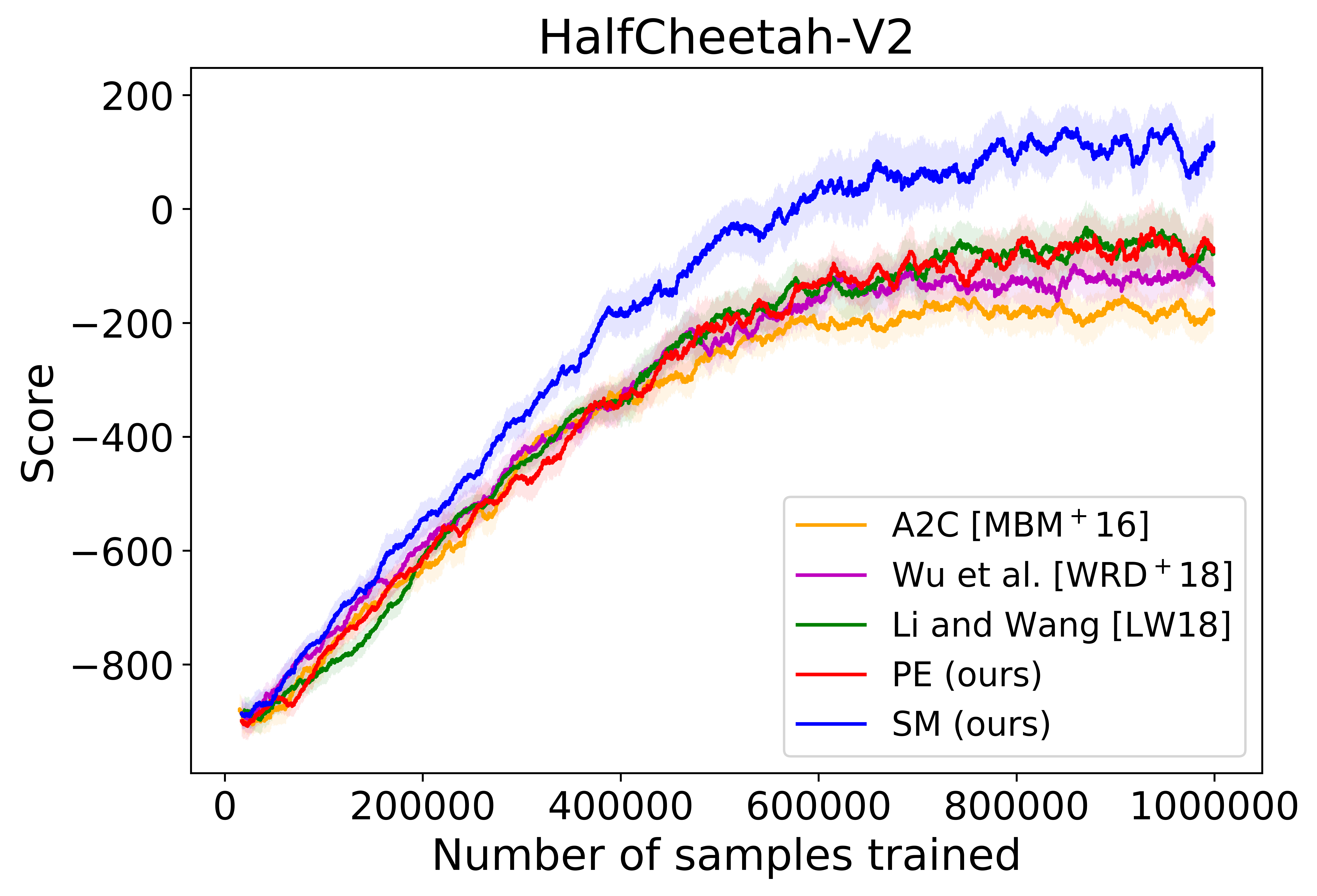
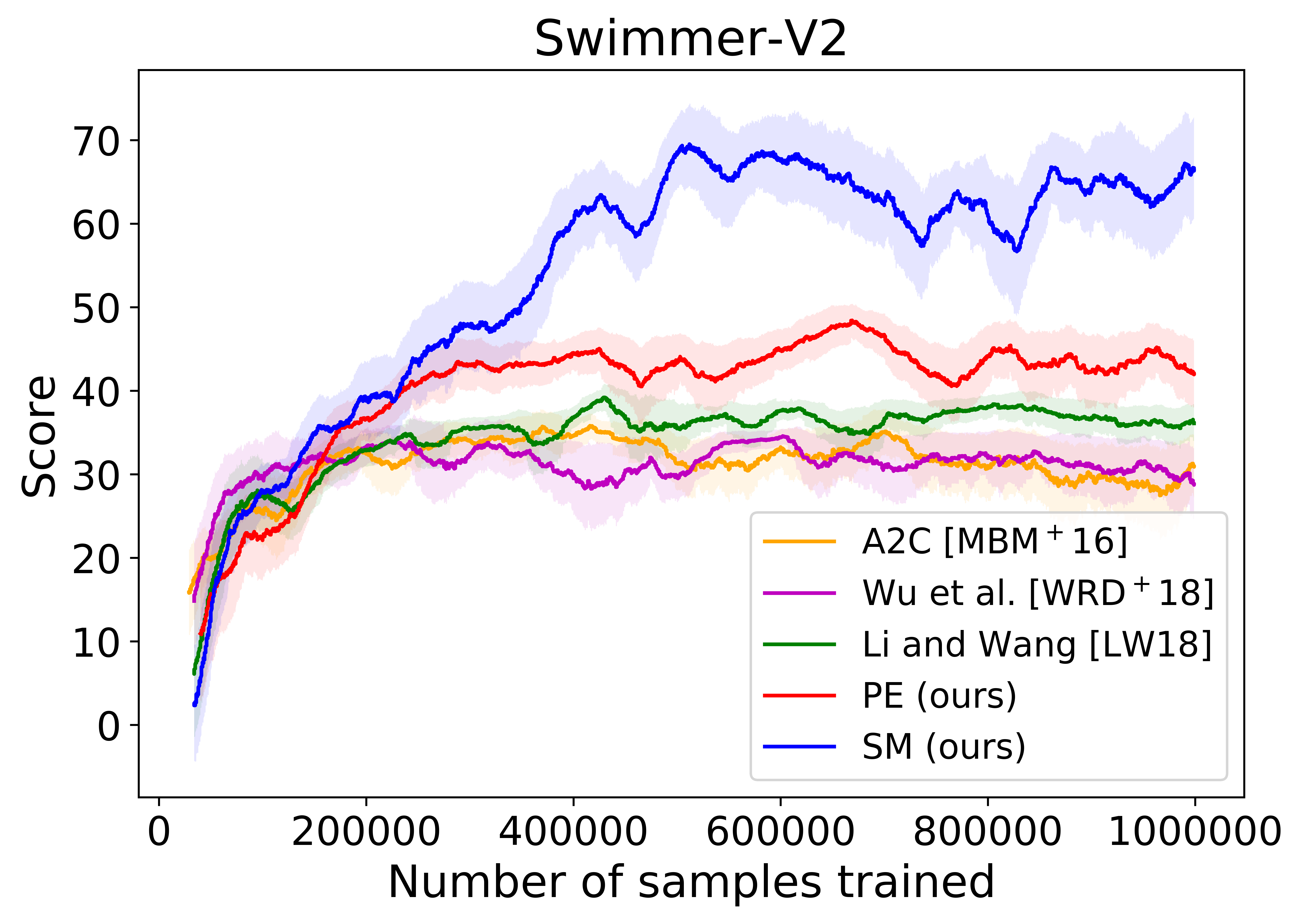
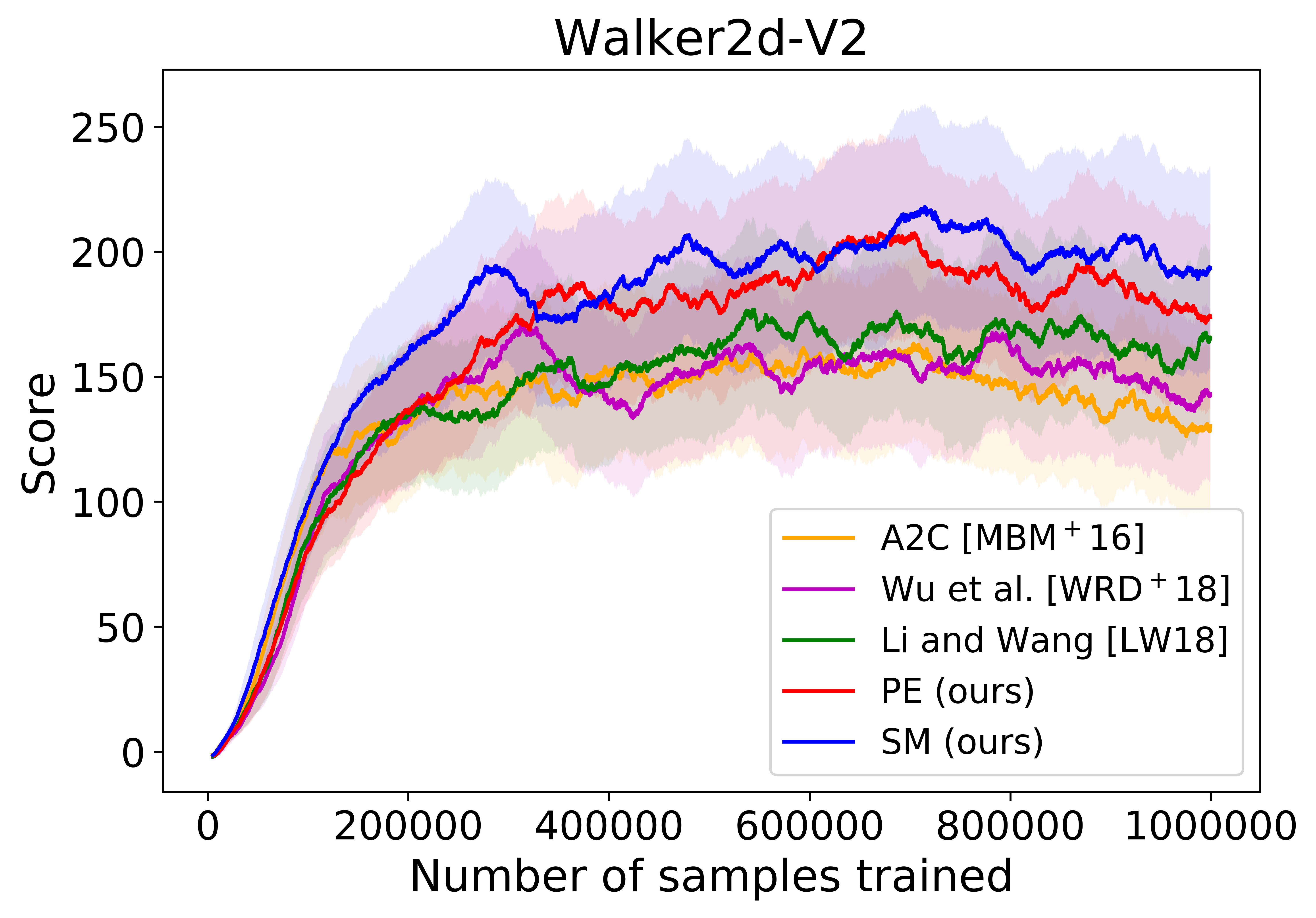
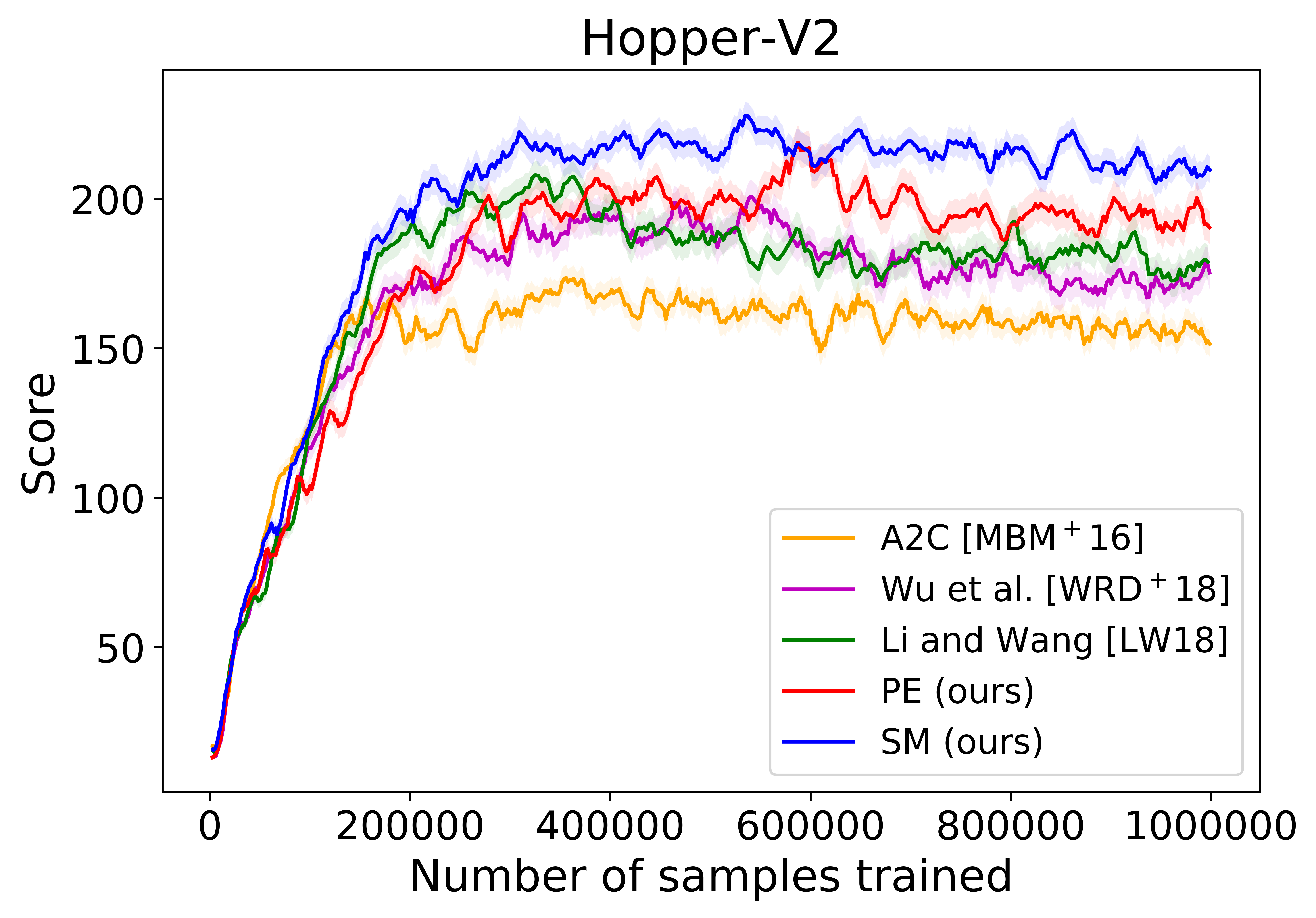
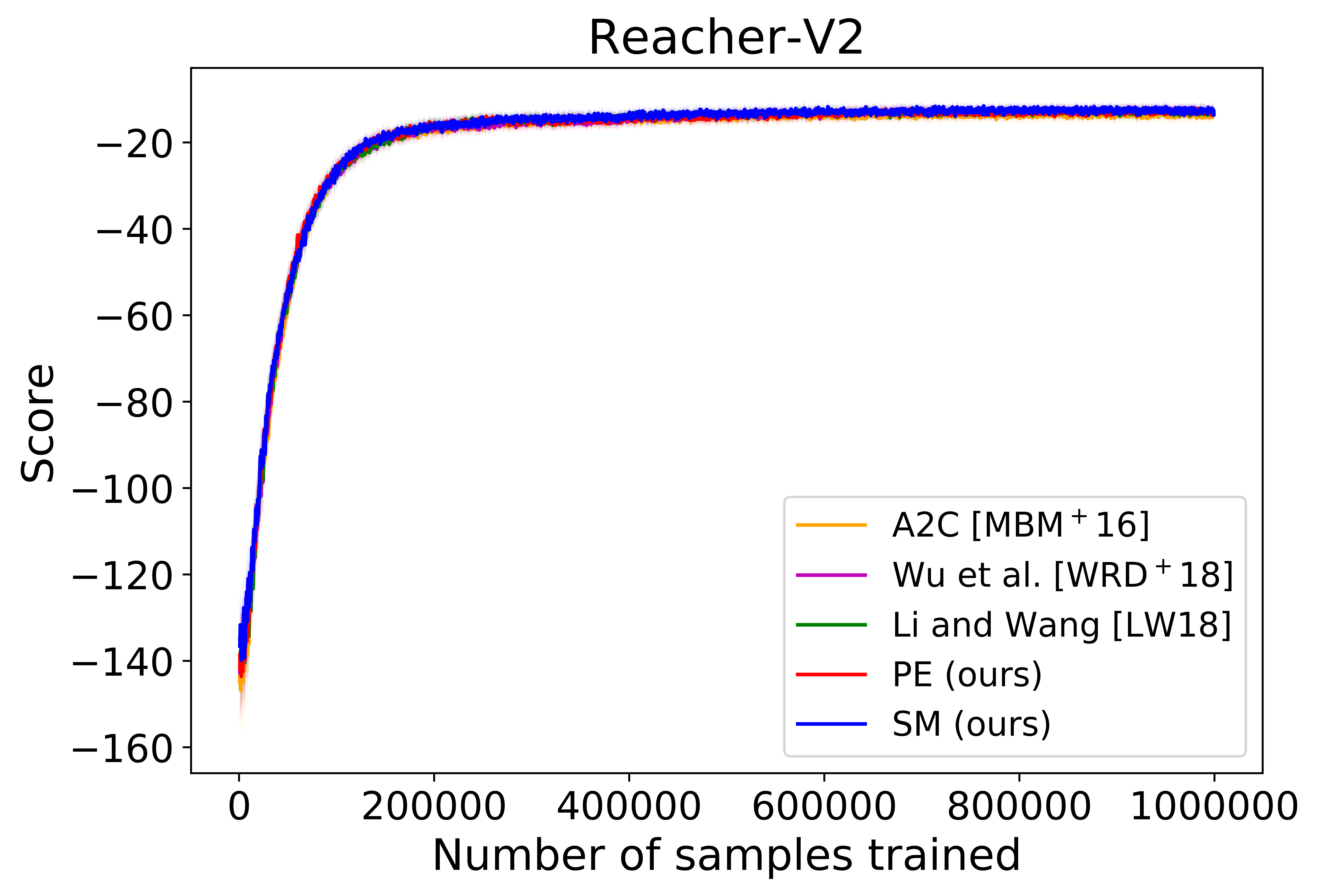
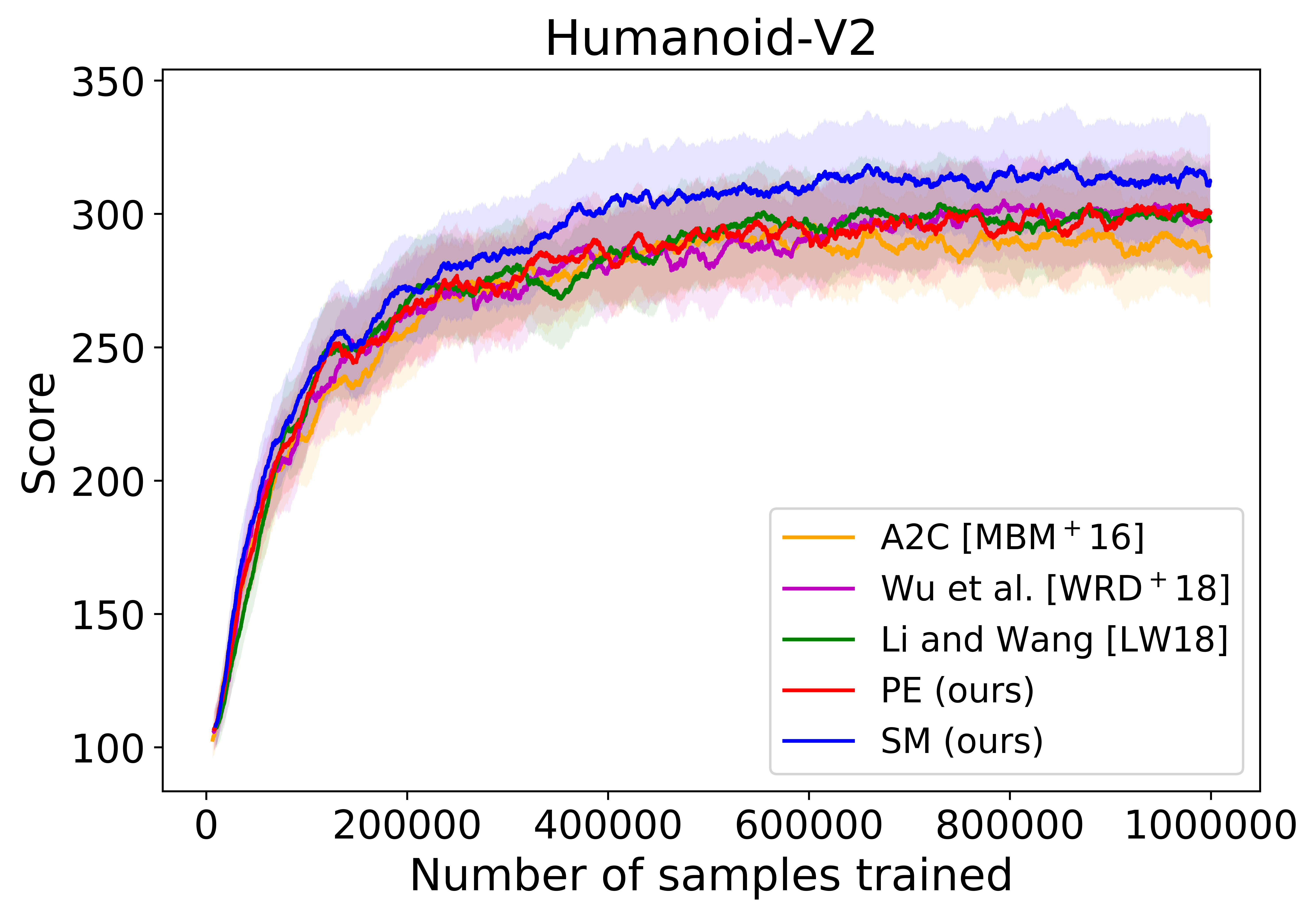
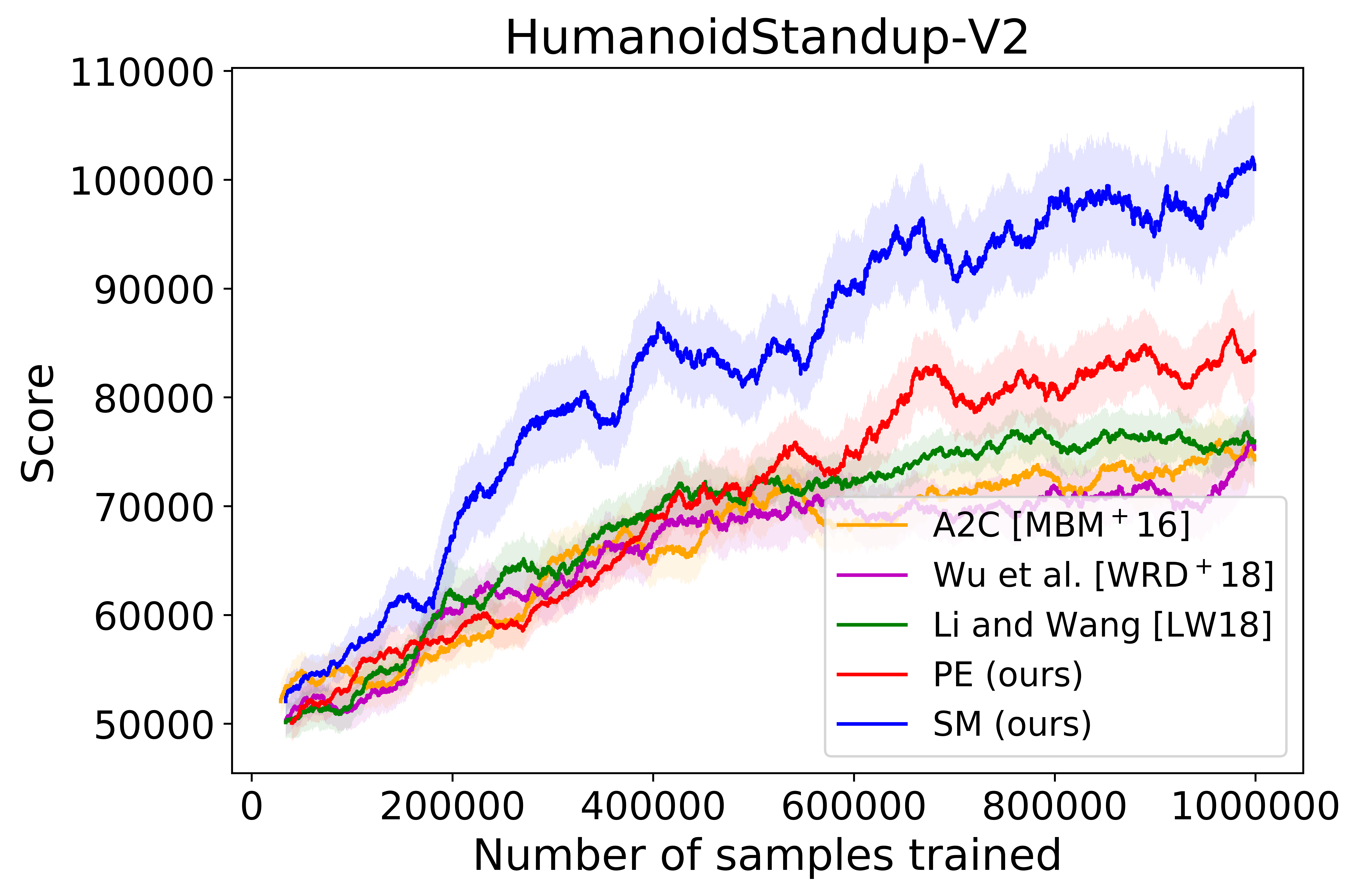
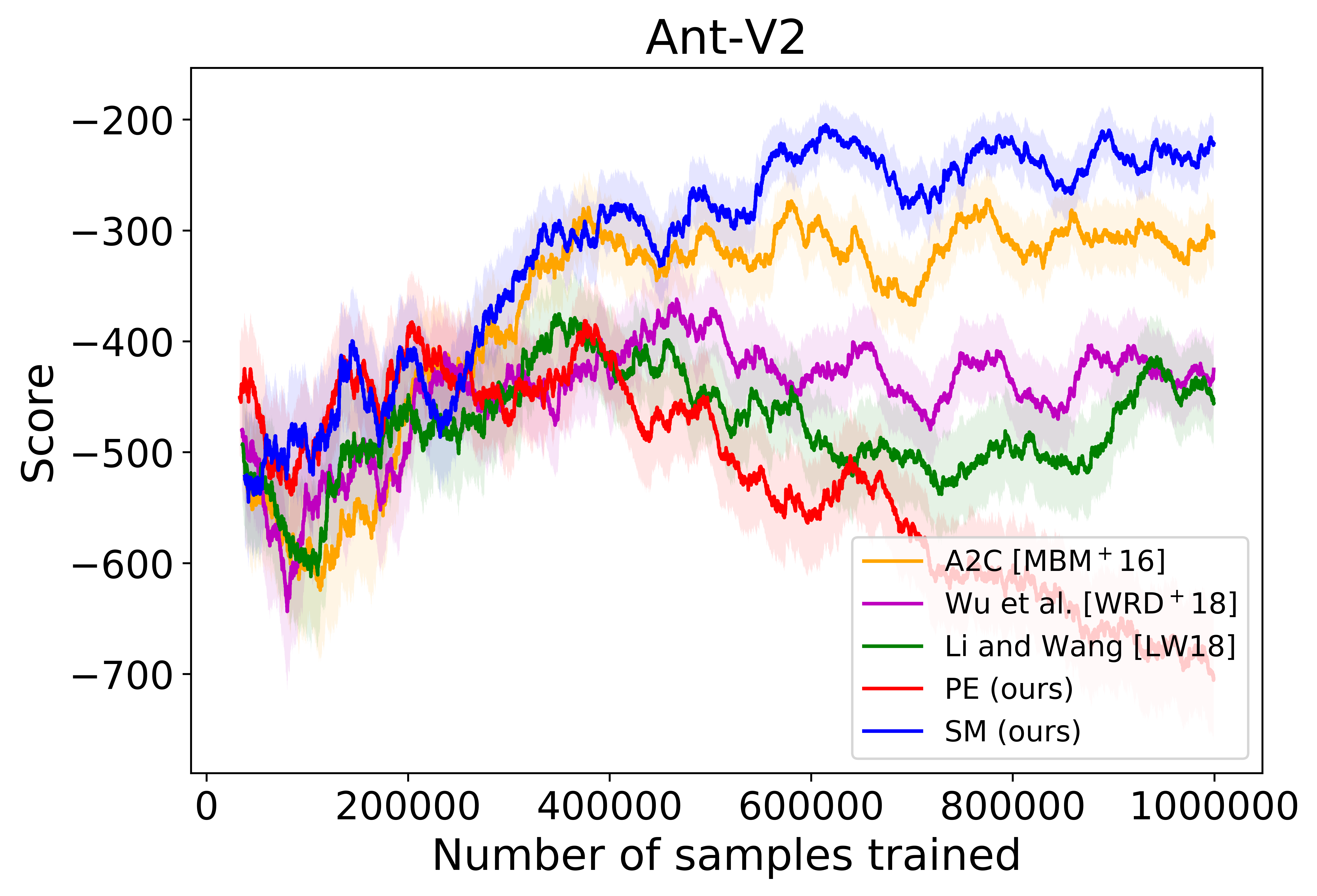
Figure 1: Empirical comparisons on MuJoCo high-dimensional control tasks. Each curve is averaged over 10 independent experiments.

Acknowledgments

We would like to thank Arnab Bhattacharyya and Guy Kindler for helpful discussions on our work and its connection to learning and testing juntas, Lap Chi Lau for telling us about the work of Blais et al. [BCE⁺18], and Jiajin Li for pointing out that variable partitioning for reinforcement learning in fact reduces the variance of its policy gradient estimator.

Appendix A Statistical claims

Claim 27.

Assume $t,\hat{t}\geq 0$. If $t^{p}\leq\hat{t}^{p}\leq t^{p}+(\varepsilon/2)^{p}$ then $t\leq\hat{t}\leq t+\varepsilon$.

Proof.

The left-hand inequalities are immediate. For the right-hand ones we start we consider two cases. If $t\leq\varepsilon/2$, then $\hat{t}^{p}\leq 2(\varepsilon/2)^{p}\leq\varepsilon\leq t+\varepsilon$. If $t>\varepsilon/2$ then

$$\hat{t}-t\leq\frac{\hat{t}^{p}-t^{p}}{t^{p-1}}\leq\frac{(\varepsilon/2)^{p}}{(\varepsilon/2)^{p-1}}\leq\varepsilon.\hfill$$

Claim 7.

Assuming $\|F\|_{\mathbb{R},2p}\leq 1$, the value $\|F\|_{\mathbb{R},p}^{p}$ can be estimated within $\varepsilon^{p}$, and $\|F\|_{\mathbb{R},p}$ can be estimated within $\varepsilon$, from $K^{p}{\log(1/\gamma)}/{\epsilon^{2p}}$ queries to $F$ in linear time with probability $1-\gamma$ for some absolute constant $K$.

Proof.

By Chebyshev’s inequality, $\mathbb{E}[\lvert F\rvert^{p}]$ can be estimated within an additive error of $(\varepsilon/2)^{p}$ by averaging $(2/\varepsilon)^{2p}$ samples with probability $3/4$. The error can be improved to $1-\gamma$ by taking the median value of $\mathcal{O}(\log 1/\gamma)$ runs. The second bound follows from Claim 27. ∎

Appendix B Details in the experiments

The exact reinforcement learning control algorithm we used is described below. The algorithm is based on proximal policy optimization [SWD⁺17] and generalized advantage estimator [SML⁺15, DWS12] in reinforcement learning.

Algorithm 5 Policy optimization with variable partitions

1:Input: Total number of samples $T$, batch size $B$, partition frequency $M_{p}$, number of value iterations $M_{w}$, initial policy parameter $\theta$, initial value and advantage parameters $w$ and $\mu$;

2:Output: Optimized policy $\pi_{\theta}$;

3:for each iteration $j$ in $[T/B]$ do

4:     Collect a batch of trajectory data $\{s_{t}^{(i)},a_{t}^{(i)},r_{t}^{(i)}\}_{i=1}^{B}$;

5:     for $M_{\theta}$ iterations do

6:         Update $\theta$ by one gradient descent step using proximal policy gradient with the gradient estimator (12);

7:     end for

8:     for $M_{w}$ iterations do

9:         Update $w$ and $\mu$ by minimizing $\|V^{w}(s_{t})-R_{t}\|_{2}^{2}$ and $\|\hat{A}-A^{\mu}(s_{t},a_{t})\|_{2}^{2}$ in one step;

10:     end for

11:     Estimate $\hat{A}(s_{t},a_{t})$ using $V^{w}(s_{t})$ by generalized advantage estimator;

12:     if $j\equiv 0\;(\bmod\;M_{p})$ then

13:         Define random function $\xi(\bm{X})$ to be an estimation of $\mathbb{E}[D_{F}(\bm{X},\bm{\overline{X}})^{2}]$;

14:         Run submodular minimization over $\bm{X}$ on $\xi(\bm{X})$;

15:         Assign $\bm{X}$ and $\bar{\bm{X}}$ to $a_{(1)}$ and $a_{(-1)}$ in (12), respectively;

16:     end if

17:end for

The differences between our algorithm and proximal policy gradient [SWD⁺17] have been highlighted: Line 6 uses the estimator with partitions on the control variables. Line $12$-$16$ find the near-optimal variable partition using submodular minimization, by Theorem 2.

We use three neural networks as function approximations: a policy network $\pi_{\theta}$ and a value network $V^{w}$ as is in the baseline methods, and an advantage network $A^{\mu}$ solely used in the partition algorithm. The networks have the same architecture as is in the previous line of works [MBM⁺16, SWD⁺17].

In our MuJoCo experiments, the tasks have been slightly modified (the physics simulator keeps intact). As the number of control variables of the original tasks is relatively low, we augment such dimensions by letting the agent controls two independent instances of the tasks at the same time. The scores and the reinforcement signals are then the additions of the scores of the two sub-tasks. Correspondingly, we use $k=2$ in [LW18] and our algorithms.

References

- [BCE+18] Eric Blais, Clément L Canonne, Talya Eden, Amit Levi, and Dana Ron. Tolerant junta testing and the connection to submodular optimization and function isomorphism. In Proceedings of the Twenty-Ninth Annual ACM-SIAM Symposium on Discrete Algorithms, pages 2113–2132. Society for Industrial and Applied Mathematics, 2018.
- [BCP+16] Greg Brockman, Vicki Cheung, Ludwig Pettersson, Jonas Schneider, John Schulman, Jie Tang, and Wojciech Zaremba. Openai gym. arXiv preprint arXiv:1606.01540, 2016.
- [Bla09] Eric Blais. Testing juntas nearly optimally. In Proceedings of the 41st Annual ACM Symposium on Theory of Computing, STOC 2009, Bethesda, MD, USA, May 31 - June 2, 2009, pages 151–158, 2009.
- [Bsh19] Nader H. Bshouty. Almost optimal distribution-free junta testing. In 34th Computational Complexity Conference, CCC 2019, July 18-20, 2019, New Brunswick, NJ, USA, pages 2:1–2:13, 2019.
- [BU87] S.S. Barsov and Vladimir Ulyanov. Estimates of the proximity of gaussian measures. Doklady Mathematics, 34:462–, 01 1987.
- [CG04] Hana Chockler and Dan Gutfreund. A lower bound for testing juntas. Inf. Process. Lett., 90(6):301–305, 2004.
- [CL15] Chandra Chekuri and Shi Li. A note on the hardness of approximating the -way hypergraph cut problem, 2015.
- [CR96] George Casella and Christian P Robert. Rao-blackwellisation of sampling schemes. Biometrika, 83(1):81–94, 1996.
- [CST+18] Xi Chen, Rocco A. Servedio, Li-Yang Tan, Erik Waingarten, and Jinyu Xie. Settling the query complexity of non-adaptive junta testing. J. ACM, 65(6):40:1–40:18, November 2018.
- [CXY18] Karthekeyan Chandrasekaran, Chao Xu, and Xilin Yu. Hypergraph k-cut in randomized polynomial time. In Proceedings of the Twenty-Ninth Annual ACM-SIAM Symposium on Discrete Algorithms, SODA ’18, pages 1426–1438, Philadelphia, PA, USA, 2018. Society for Industrial and Applied Mathematics.
- [DDG+17] Roee David, Irit Dinur, Elazar Goldenberg, Guy Kindler, and Igor Shinkar. Direct sum testing. SIAM Journal on Computing, 46(4):1336–1369, 2017.
- [DG19] Irit Dinur and Konstantin Golubev. Direct sum testing: The general case. In Approximation, Randomization, and Combinatorial Optimization. Algorithms and Techniques, APPROX/RANDOM 2019, September 20-22, 2019, Massachusetts Institute of Technology, Cambridge, MA, USA, pages 40:1–40:11, 2019.
- [DWS12] Thomas Degris, Martha White, and Richard S Sutton. Off-policy actor-critic. arXiv preprint arXiv:1205.4839, 2012.
- [FKR+04] Eldar Fischer, Guy Kindler, Dana Ron, Shmuel Safra, and Alex Samorodnitsky. Testing juntas. Journal of Computer and System Sciences, 68(4):753–787, 2004.
- [GLS81] Martin Grötschel, László Lovász, and Alexander Schrijver. The ellipsoid method and its consequences in combinatorial optimization. Combinatorica, 1(2):169–197, 1981.
- [IO09] Satoru Iwata and James Orlin. A simple combinatorial algorithm for submodular function minimization. In Proceedings of the Annual ACM-SIAM Symposium on Discrete Algorithms, pages 1230–1237, 01 2009.
- [Kar00] David R. Karger. Minimum cuts in near-linear time. J. ACM, 47(1):46–76, January 2000.
- [Kos18] Ilya Kostrikov. Pytorch implementations of reinforcement learning algorithms. https://github.com/ikostrikov/pytorch-a2c-ppo-acktr, 2018.
- [KS96] David R. Karger and Clifford Stein. A new approach to the minimum cut problem. J. ACM, 43(4):601–640, July 1996.
- [KS09] Marek Karpinski and Warren Schudy. Linear time approximation schemes for the gale-berlekamp game and related minimization problems. In Proceedings of the Forty-first Annual ACM Symposium on Theory of Computing, STOC ’09, pages 313–322, New York, NY, USA, 2009. ACM.
- [KSL15] David Karger and Matthew S. Levine. Fast augmenting paths by random sampling from residual graphs. SIAM Journal on Computing, 44:320–339, 03 2015.
- [KT15] Ken-ichi Kawarabayashi and Mikkel Thorup. Deterministic global minimum cut of a simple graph in near-linear time. In Proceedings of the Forty-seventh Annual ACM Symposium on Theory of Computing, STOC ’15, pages 665–674, New York, NY, USA, 2015. ACM.
- [KW96] Regina Klimmek and Frank Wagner. A simple hypergraph min cut algorithm, 1996. Technical Report B.
- [LSW15] Yin Tat Lee, Aaron Sidford, and Sam Chiu-wai Wong. A faster cutting plane method and its implications for combinatorial and convex optimization. In 2015 IEEE 56th Annual Symposium on Foundations of Computer Science, pages 1049–1065. IEEE, 2015.
- [LW18] Jiajin Li and Baoxiang Wang. Policy optimization with second-order advantage information. arXiv preprint arXiv:1805.03586, 2018.
- [Man17] Pasin Manurangsi. Almost-polynomial ratio ETH-hardness of approximating densest -subgraph. In Proceedings of the 49th Annual ACM SIGACT Symposium on Theory of Computing, STOC 2017, pages 954–961, New York, NY, USA, 2017. ACM.
- [MBM+16] Volodymyr Mnih, Adria Puigdomenech Badia, Mehdi Mirza, Alex Graves, Timothy P Lillicrap, Tim Harley, David Silver, and Koray Kavukcuoglu. Asynchronous methods for deep reinforcement learning. In International Conference on Machine Learning, 2016.
- [MOOS03] Elchanan Mossel, Ryan O’Donnell, Ryan O’Donnell, and Rocco P Servedio. Learning juntas. In Proceedings of the thirty-fifth annual ACM symposium on Theory of computing, pages 206–212. ACM, 2003.
- [Que98] Maurice Queyranne. Minimizing symmetric submodular functions. Mathematical Programming, 82(1-2):3–12, 1998.
- [RSW18] Aviad Rubinstein, Tselil Schramm, and S. Matthew Weinberg. Computing Exact Minimum Cuts Without Knowing the Graph. In Anna R. Karlin, editor, 9th Innovations in Theoretical Computer Science Conference (ITCS 2018), volume 94 of Leibniz International Proceedings in Informatics (LIPIcs), pages 39:1–39:16, Dagstuhl, Germany, 2018. Schloss Dagstuhl–Leibniz-Zentrum fuer Informatik.
- [RV07] R. M. Roth and K. Viswanathan. On the hardness of decoding the gale-berlekamp code. In 2007 IEEE International Symposium on Information Theory, pages 1356–1360, June 2007.
- [Sag18] Mert Saglam. Near log-convexity of measured heat in (discrete) time and consequences. In 59th IEEE Annual Symposium on Foundations of Computer Science, FOCS 2018, Paris, France, October 7-9, 2018, pages 967–978, 2018.
- [SB18] Richard S Sutton and Andrew G Barto. Reinforcement learning: An introduction. MIT press, 2018.
- [SML+15] John Schulman, Philipp Moritz, Sergey Levine, Michael Jordan, and Pieter Abbeel. High-dimensional continuous control using generalized advantage estimation. arXiv preprint arXiv:1506.02438, 2015.
- [SMSM00] Richard S Sutton, David A McAllester, Satinder P Singh, and Yishay Mansour. Policy gradient methods for reinforcement learning with function approximation. In Advances in neural information processing systems, pages 1057–1063, 2000.
- [SV95a] Huzur Saran and Vijay V Vazirani. Finding k cuts within twice the optimal. SIAM Journal on Computing, 24(1):101–108, 1995.
- [SV95b] Huzur Saran and Vijay V. Vazirani. Finding cuts within twice the optimal. SIAM J. Comput., 24(1):101–108, 1995.
- [SWD+17] John Schulman, Filip Wolski, Prafulla Dhariwal, Alec Radford, and Oleg Klimov. Proximal policy optimization algorithms. arXiv preprint arXiv:1707.06347, 2017.
- [Wil92] Ronald J Williams. Simple statistical gradient-following algorithms for connectionist reinforcement learning. Machine learning, 8(3-4):229–256, 1992.
- [WRD+18] Cathy Wu, Aravind Rajeswaran, Yan Duan, Vikash Kumar, Alexandre M.Bayen, Sham Kakade, Igor Mordatch, and Pieter Abbeel. Variance reduction for policy gradient with action-dependent factorized baselines. In International Conference on Learning Representations, 2018.