Robust Output Regulation: Optimization-Based Synthesis and Event-Triggered Implementation

Abstract.

We investigate the problem of practical output regulation, i.e., to design a controller that brings the system output in the vicinity of a desired target value while keeping the other variables bounded. We consider uncertain systems that are possibly nonlinear and the uncertainty of their linear parts is modeled element-wise through a parametric family of matrix boxes. An optimization-based design procedure is proposed that delivers a continuous-time control and estimates the maximal regulation error. We also analyze an event-triggered emulation of this controller, which can be implemented on a digital platform, along with an explicit estimates of the regulation error.

1. Introduction

Output regulation of uncertain dynamic systems is a fundamental problem in the control literature that finds a wide range of real-world applications [27]. The problem has been studied in various settings depending on the system dynamics (e.g., linear [13] or nonlinear models [23]) and uncertainty nature (e.g., characterization in time [22] or frequency domains [7]). In the light of recent developments of digitalization, communication and computation limitations of the controllers’ architecture have also become an important consideration, which also contributes to this variety of the setting. In particular, one of the distinct features of the controllers is the time scale under which the controller receives output measurements or updates the control efforts applied to the systems (e.g., continuous [13], periodic [9], or event-based interactions [37]).

From a literature point of view, the uncertainty aspect is often the focus of robust control while the time-scale implementation of the controllers is the main theme of the event-triggered mechanism. The control synthesis tools of output regulation were first developed in the robust control literature for the setting in which the uncertainty is characterized in the frequency domain [7, 18]. The setting of time-domain uncertainty, however, remains much less explored partly, due to the inherent provable computational difficulty [28]. Considering the current existing works briefly mentioned above, we set the following as our main objective in this study:

Given a nonlinear plant with element-wise time-domain uncertainty, we aim to develop a scalable computational framework, along with rigorous and explicit performance guarantees, to synthesize a robust output regulator and an event-triggered mechanism enabling its implementation on a digital platform.

Related literature on robust control

A natural way for modeling of the uncertainty in the time domain is through the state-space representation of the dynamic systems. The stability of such systems can be cast as an optimization program, which unfortunately is often computationally intractable [10]. Conservative approximations in the form of linear matrix inequalities (LMIs) are proposed for particular subclasses of uncertainty including single ellipsoid [34] or polytopic systems with low number of vertices [13, 14, 1]. A richer modeling framework is element-wise or box uncertainty that allows to conveniently incorporate different sources of uncertainties. One approach to deal with this class of uncertainty is randomized algorithms [35]. Alternatively, one can leverage the recent developments in the robust optimization literature [4] to address the computational bottleneck. The optimization-based framework proposed in this paper exploits the latter result in the context of output regulation.

Related literature on event-triggered control of uncertain systems

The second part of this study is concerned with event-triggered control, as a powerful technique to address the potential communication limitation on the measurement or actuation side. A recent approach towards event-triggered control of uncertain systems builds on an adaptive control perspective [37, 36]. The structure of an event triggering mechanism dictated by the necessity to maintain a positive dwell time between consecutive events usually makes it impossible to ensure asymptotic convergence. As such, the practical stability (i.e., convergence to a “tunable” invariant set) is aimed for. Such a notion is also adopted in other contexts like quantized control [5], and has been investigated in the presence of a common Lyapunov function [22, 23].

Focusing on uncertain linear systems, the work [34] considers norm-bounded uncertainties with continuous measurements, while [24, 30] develop mechanism under the assumption that the system is minimum-phase. Most recently, the work [21] studies the problem of output regulation together along with an event-triggering mechanism in which the robustness is guaranteed for an unstructured open uncertainty set. Concerning nonlinear systems, the recent work [16] proposes an event-triggered mechanism under the assumption that the system is input-to-state stable. Unlike the existing literature mentioned above, in this article we opt to introduce an event-triggering mechanism in which both monitoring the output measurement and implementing the actuation values operate on a discrete-time basis. To our best knowledge, none of the existing works considers this setting in control of uncertain nonlinear systems. The closest work in this spirit is [39], in which the class of single-input single-output system is considered and the performance is guaranteed only for sufficiently large feedback gains and sufficiently small periodic sampled-times.

Our contributions

The particular emphasis of this study is on the computational aspect of the control design and the corresponding event-triggering mechanism, along with explicit performance guarantees. More specifically, the contributions of the article are summarized as follows:

1. Dynamic structure and inherent hardness: We propose a class of dynamic output controllers aiming to locate the closed-loop equilibrium in accordance with the desired regulation task (Section 3.1 and Lemma 3.1). We further show that from a computational viewpoint stability analysis of the proposed controller is strongly NP-hard (Proposition 3.2).

2. Robust control under element-wise (box) uncertainties: We provide a sufficient condition along with an optimization framework to synthesize a dynamic output controller that enjoys a provable practical stability (Theorem 3.3). As a byproduct, we also show that given any fixed controller, the proposed optimization program reduces to a tractable convex optimization that can be viewed as a computational certification tool for the practical stability (Corollary 3.4).

3. Sampled-time event-triggered mechanism: We propose a unifying triggering mechanism together with easy-to-compute sufficient conditions under which the proposed output controller can be implemented through aperiodic measurements and event-based actuation (Theorem 4.2). The proposed mechanism offers explicit computable maximal inter-sampling and regulation error bounds. The proposed result subsumes both the existing approaches [33, 12] as a special case (Corollary 4.5 and Remark 4.3).

4. Numerical algorithm: Leveraging recent results from [20], we propose a numerical algorithm to deal with nonlinearities of the proposed optimization program concerning the control synthesis of the output regulation task (Algorithm 2).

In the rest of the article, we present a formal description of the problem along with some basic assumptions in Section 2. The robust control method is developed in Section 3, and the sampled-time event-triggered mechanism is presented in Section 4. Section 5 discusses an algorithm to tackle the proposed optimization program, and further provides numerical example in order to validate the theoretical results.

Notation

The set of $n\times n$ symmetric matrices and the set of $n\times n$ positive-definite (semi-definite) symmetric ones are denoted by $\mathbb{S}^{n}$ and $\mathbb{S}^{n}_{\succ 0}$ ($\mathbb{S}^{n}_{\succeq 0}$), respectively. For two symmetric matrices $A$ and $B$, we write $A\succ B$ (respectively, $A\succeq B$) if $A-B\in\mathbb{S}^{n}_{\succ 0}$ (respectively, $\mathbb{S}^{n}_{\succeq 0}$). For a square matrix $A$, we denote $\left[{A}\right]^{\dagger}=A+A^{\top}$. The symbol $\mathfrak{Diag}\left\{{A_{1},A_{2},...,A_{n}}\right\}$ denotes the block diagonal matrix with blocks $A_{1},A_{2},...,A_{n}$. For briefness in notations, the matrix $\begin{bmatrix}A&B^{\top}\\ B&C\end{bmatrix}$ is shown by $\begin{bmatrix}A&*\\ B&C\end{bmatrix}$. We use $e_{1},\ldots,e_{m}$ to denote the standard coordinate basis of $\mathbb{R}^{m}$. Also, $\mathds{1}_{m}\in\mathbb{R}^{m}$ denotes the vector whose elements are all equal to $1$.

2. Problem Statement

Consider the control system

$$\left\{\begin{array}[]{l}\dot{x}(t)=A^{\star}x(t)+B^{\star}u(t)+k^{\star}\big{(}x(t)\big{)}\vspace{1mm}\\ y(t)=Cx(t)\end{array}\right.$$ (1)

where the vector $x(t)\in\mathbb{R}^{{n_{x}}}$, $u(t)\in\mathbb{R}^{{n_{u}}}$, and $y(t)\in\mathbb{R}^{{n_{y}}}$ are the state, the control, and the output vectors, respectively. The matrices $A^{\star}$ and $B^{\star}$ represent the linear part of the state dynamics, and the function $k^{\star}:\mathbb{R}^{n_{x}}\rightarrow\mathbb{R}^{n_{x}}$ encapsulates the nonlinearity of the dynamics. Throughout this article, we assume that system (1) admits a unique solution $x(\cdot)$ for any $x(0)$. The controller to be designed in the next section has access only to the output $y(t)$. We allow the matrices $A^{\star},B^{\star}$ and the nonlinearity $k^{\star}:\mathbb{R}^{n_{x}}\rightarrow\mathbb{R}^{n_{x}}$ in the system (1) to be partially uncertain. Our main control objective is to stabilize (1) in the Lagrange sense (i.e., all solutions are bounded) and steer the output trajectory of (1) to an $\varepsilon$-neighborhood of a target value $y^{\rm d}\in\mathbb{R}^{n_{y}}$. Formally speaking, we aim to ensure that

$$\sup_{t\geq 0}\|x(t)\|<\infty,\;\;\varlimsup_{t\to\infty}\|y(t)-y^{\rm d}\|\leq\varepsilon\quad\forall x(0)\in\mathbb{R}^{n_{x}}.$$ (2)

The special case of $\varepsilon=0$ corresponds to asymptotic output regulation and the relaxed condition with is known as “$\varepsilon$-practical output stability” [26].

Henceforth, the following assumptions are adopted.

Assumption 2.1.

[Uncertainty characterization] System (1) and the desired value $y^{\rm d}\in\mathbb{R}^{n_{y}}$ satisfy the following assumptions:

1. (Box uncertainty) Matrices $A^{\star}$ and $B^{\star}$ obey inequalities

   $$|A^{\star}-A|\leq A_{b},\quad|B^{\star}-B|\leq B_{b},$$ (3)

   where $A$ and $B$ are known nominal matrices, the inequalities are understood element-wise, and $A_{b}=\begin{bmatrix}a_{b_{ij}}\end{bmatrix}_{ij},B_{b}=\begin{bmatrix}b_{b_{ij}}\end{bmatrix}_{ij}$ are the respective uncertainty bounds.

2. (Bounded nonlinearity) The function $k^{\star}$ satisfies

   $$\|k^{\star}(x_{1})-k^{\star}(x_{2})\|\leq k_{b},\qquad\forall x_{1},x_{2}\in\mathbb{R}^{n_{x}}$$ (4)

   where $k_{b}\geq 0$ is a known constant.

3. (Existence of an equilibrium) There exists a pair $(x^{\rm d},u^{\rm d})\in\mathbb{R}^{n_{x}}\times\mathbb{R}^{n_{u}}$ such that

   $$y^{\rm d}=Cx^{\rm d}\quad\textrm{and}\quad A^{\star}x^{\rm d}+k^{\star}(x^{\rm d})=-B^{\star}u^{\rm d}\,.$$ (5)

Assumption 2.1(ii) holds if and only if the nonlinearity of the dynamics is globally bounded. If $\|k^{\star}(x)\|\leq C$, then (4) holds with $k_{b}=2C$. However, this estimate of $k_{b}$ may be too conservative, e.g., if $k^{\star}$ is an uncertain constant, one can actually choose $k_{b}=0$. The “incremental” condition (4) thus provides more flexbility. There are several classes of nonlinear dynamics for which the bound (4) is available: (i) pendulum-like nonlinearity which represents periodicity of the dynamics, e.g., phase-locked loops [38, 32], or swing equations in power systems [25]; (ii) nonlinearity presented due to an underlying neural network architecture [8] or a lookup-table [11]. Such nonlinearities may or may not be fully known, but regardless of this knowledge, it is often too complicated to be utilized in control synthesis algorithms. Furthermore, we emphasize that the bound $k_{b}$ will not be required for control design and is only used in the final performance bounds.

Assumption 2.1(iii) involves $({n_{y}}+{n_{x}})$ algebraic constraints with $({n_{x}}+{n_{u}})$ variables. Therefore, we typically expect that such equations have a solution $(x^{\rm d},u^{\rm d})$ when ${n_{u}}\geq{n_{y}}$, i.e., the number of control variables is not less than the number of outputs. When the dynamic system (1) is linear (i.e., $k^{*}$ is constant), these equations reduce to a set of linear constraints, and that a sufficient condition for Assumption 2.1(iii) is the matrix $\begin{bmatrix}C&0\\ A^{\star}&B^{\star}\end{bmatrix}$ of full column rank.

Problem 2.2.

Consider the system (1) under Assumption 2.1, and let $y^{\rm d}\in\mathbb{R}^{n_{y}}$ and $\varepsilon\geq 0$ be a desired target and regulation precision, respectively.

1. Control synthesis: Synthesize an output control $y_{[0,t]}\mapsto u(t)$, $t\geq 0$, in order to ensure the $\varepsilon$-practical output regulation in the sense of (2).

2. Sampled-time event-based emulation: Given a prescribed series of measurement sampled-times, design a triggering mechanism to update the control along with a guaranteed precision of the desired output regulation (2).

We start with designing a continuous-time controller (Section 3) whose sampled-time redesign, or emulation, is considered in Section 4. Note that the viability of the sampled-time emulation reflects a certain robustness level of the continuous-time controller.

3. Continuous-Time Control Design

The main focus of this section is Problem 2.2(i). We first find a structure of the controller ensuring that the closed-loop system has an equilibrium $(x^{\rm d},u^{\rm d})$ such that $y^{\rm d}=Cx^{\rm d}$, and then provide sufficient conditions guaranteeing that this equilibrium is globally asymptotically stable. The existence of an equilibrium is natural, if one is interested in the $\varepsilon$-practical stability (2) with an arbitrarily small $\varepsilon$.

A possible control architecture, and perhaps the simplest form, is the static controller $u(t)=D_{c}y(t)+\eta$. Unfortunately, to provide the existence of an equilibrium from Assumption 2.1(iii), the parameter $\eta=u^{\rm d}-D_{c}y^{\rm d}$ should depend on $u^{\rm d}$, which, in turn, depends on the uncertain matrices $A^{\star}$ and $B^{\star}$ and function $k^{\star}$. For this reason, we propose a dynamic controller, being a multidimensional counterpart of the classical proportional-integral control.

3.1. Dynamic control and equilibrium existence

Consider now a more general dynamic controller

$$\begin{dcases}\dot{w}(t)=A_{c}w(t)+B_{c}y(t)+\xi\\ u(t)=C_{c}w(t)+D_{c}y(t)+\eta,\end{dcases}$$ (6)

where matrices $A_{c},C_{c}\in\mathbb{R}^{{n_{u}}\times{n_{u}}}$, $B_{c},D_{c}\in\mathbb{R}^{{n_{u}}\times{n_{y}}}$ and $\xi,\eta\in\mathbb{R}^{{n_{u}}}$ are the design parameters. These additional parameters in (6) enable one to make the equilibrium $(x^{*},w^{*})$ of the closed-loop system (1) and (6) compatible with the target value $y^{\rm d}$ in the face of the parametric uncertainty (3).

Lemma 3.1 (Closed-loop equilibrium).

If Assumption 2.1(iii) holds, the matrix $C_{c}$ has full column rank, and the controller parameters are such that

$$A_{c}=0\quad\textrm{and}\quad\xi=-B_{c}y^{\rm d},\,$$ (7)

then the closed-loop system (1) and (6) has an equilibrium $(x^{\rm d},w^{\rm d})$, where $x^{\rm d}$ is introduced in Assumption 2.1(iii).

Proof.

Since the matrix $C_{c}$ has full column rank, there exists $w^{\rm d}\in\mathbb{R}^{n_{u}}$ such that $C_{c}w^{\rm d}+D_{c}y^{\rm d}+\eta=u^{\rm d}$, where $u^{\rm d}$ is given by (5). In view of Assumption 2.1(iii) and (7), the point $(x^{d},w^{d})\in\mathbb{R}^{{n_{x}}+{n_{u}}}$ obeys the algebraic equations

$$\left\{\begin{matrix}[l]A^{\star}x^{\rm d}+B^{\star}(C_{c}w^{\rm d}+D_{c}Cx^{\rm d}+\eta)+k^{\star}(x^{\rm d})=0,\vspace{1mm}\\ A_{c}w^{\rm d}+B_{c}Cx^{\rm d}+\xi=B_{c}(y^{\rm d}-Cx^{\rm d})=0,\end{matrix}\right.$$ (8)

Hence, it is an equilibrium for the closed-loop system. ∎

Notice that the controller’s parameters $B_{c},D_{c}$, and $\eta$ do not influence the existence of an equilibrium compatible with the desired output $y^{\rm d}$. While $B_{c}$ and $D_{c}$ may influence the stability of the transient behavior of the closed-loop system, the vector $\eta$ does not affect stability and only determines $w^{d}$. Hence, without loss of generality, we set $\eta=-D_{c}y^{\rm d}$. Combining this with (7) and the controller (6) shapes into

$$\left\{\begin{matrix}[l]\dot{w}(t)=B_{c}\big{(}y(t)-y^{\rm d}\big{)}\vspace{1mm}\\ u(t)=C_{c}w(t)+D_{c}\big{(}y(t)-y^{\rm d}\big{)}\,.\end{matrix}\right.$$ (9)

Note that the dynamic controller (9) may be considered as a (multidimensional) extension of the conventional PI controller.

3.2. Closed-loop stability of transient behavior

The goal of this section is to design the controller parameters $B_{c},C_{c}$, and $D_{c}$ such that the equilibrium from Lemma 3.1 is (practically) stable. To this end, we introduce the augmented state vector of the closed-loop system as

$$z(t)\coloneqq\begin{bmatrix}x(t)-x^{\rm d}\\ w(t)-w^{\rm d}\end{bmatrix}.$$ (10)

Based on the system dynamics in (1) together with the controller (9), it is obtained that

$$\begin{array}[]{r}\dot{z}=\left[\bar{A}+J^{\top}\Delta AJ+(\bar{B}+J^{\top}\Delta BJ)F\bar{C}\right]z+J^{\top}(k^{\star}(J^{\top}z)-k^{\star}(x^{\star})),\end{array}$$ (12)

where $\Delta A=A^{\star}-A$ and $\Delta B=B^{\star}-B$ represent the uncertainty in the linear part of the system dynamics, and matrices $\bar{A},\bar{B},\bar{C},F$, and $J$ are defined as follows.

$$\begin{matrix}[l]\bar{A}\coloneqq\begin{bmatrix}A&0\\ 0&0\end{bmatrix},\,\bar{B}\coloneqq\begin{bmatrix}B&0\\ 0&I\end{bmatrix},\,\bar{C}\coloneqq\begin{bmatrix}C&0\\ 0&I\end{bmatrix},\,J\coloneqq\begin{bmatrix}I_{{n_{x}}}&0_{{n_{x}}\times{n_{u}}}\end{bmatrix},\,F\coloneqq\begin{bmatrix}D_{c}&C_{c}\\ B_{c}&0\end{bmatrix}\end{matrix}$$ (13)

It should be noted that matrix $F$ collects all the design variables of the controller. The goal of the controller design is to guarantee the (practical) stability of the system (12) for all uncertainties $\Delta A,\Delta B$, and $k^{\star}(\cdot)$ that meet Assumption 2.1. Unfortunately, it turns out that the exact characterization of such an $F$ is provably intractable. In fact, the special case of checking the stability of the system (12) for a given $F$ is also a difficult problem. This is formalized in the next proposition.

Proposition 3.2 (Intractability).

Consider the system (1) under Assumption 2.1, and let the control signal follow the dynamics (9). Then, for a given set of the control parameters (i.e., matrix $F$ in (13)), the problem of checking whether the output target stability (2) holds for some $\varepsilon\geq 0$ is strongly NP hard and equivalent to

$$\begin{matrix}[l]\forall\Delta A,\Delta B:|\Delta A|\leq A_{b},\,|\Delta B|\leq B_{b}\,\quad\exists P\in S^{{n_{x}}+{n_{u}}}_{\succ 0}:\\ \left[{P\left(\bar{A}+J^{\top}\Delta AJ\right.\left.+(\bar{B}+J^{\top}\Delta BJ)F\bar{C}\right)}\right]^{\dagger}\preceq 0.\end{matrix}$$ (14)

Proof.

Recall that the nonlinear term in the dynamics (12) is uniformly bounded due to Assumption 2.1(ii). Therefore, thanks to the classical result of [15, Theorem 9.1], the stability of the system (12) is equivalent to the stability of the linear part described as

$$\dot{z}=\left[\bar{A}+J^{\top}\Delta AJ+(\bar{B}+J^{\top}\Delta BJ)F\bar{C}\right]z\,.$$ (15)

From the classical linear system theory, we know that the stability of (15) is equivalent to the existence of a quadratic Lyapunov function $V(z)=z^{\top}Pz$, where the symmetric positive definite matrix $P$ may in general depend on the uncertainty in the dynamics. This assertion can be mathematically translated to checking whether the given controller parameter $F$ satisfies (14). Note that the order of the quantifies implies that the matrix $P$ may depend on the uncertain parameter $\Delta A$ and $\Delta B$. The assertion (14) is indeed a special case of the problem of an interval matrix’s stability [28], which is proven to be strongly NP-hard [2, Corollary 2.6]. ∎

A useful technique to deal with the assertion similar to (14) is to choose a so-called common Lyapunov function [29]. Namely, we aim to find a positive-definite matrix $P$ for all possible model parameters, i.e., the assertion (14) is replaced with a more conservative requirement as follows:

$$\begin{matrix}[l]\exists P\in S^{{n_{x}}+{n_{u}}}_{\succ 0}\quad\forall\Delta A,\Delta B:|\Delta A|\leq A_{b},\,|\Delta B|\leq B_{b}\\ \left[{P\left(\bar{A}+J^{\top}\Delta AJ\right.\left.+(\bar{B}+J^{\top}\Delta BJ)F\bar{C}\right)}\right]^{\dagger}\preceq 0.\end{matrix}$$ (16)

Note that the only difference between (14) and the conservative assertion in (16) is the order of quantifiers between the Lyapunov matrix $P$ and the linear dynamics uncertainties $\Delta A$ and $\Delta B$. The argument (16) is a special subclass of problems known as the “matrix cube problems” [3]. While this class of problems is also provably hard [3, Proposition 4.1], the state-of-the-art in the convex optimization literature offers an attractive sufficient condition where the resulting conservatism is bounded independently of the size of the problem [4]. Building on these developments, we will provide an optimization framework to design the controller parameters along with a corresponding common Lyapunov function.

Theorem 3.3 (Robust control & common Lyapunov function).

Consider the system (1), satisfying Assumption 2.1, and the controller (9). Also, consider the optimization program

$$\left\{\begin{matrix}[l]\max\hskip 5.69054pt{\alpha\zeta^{-1}}\\ \vspace{1mm}~{}{\rm s.t.}\hskip 8.53581pt\alpha\in\mathbb{R},\quad{\zeta},\kappa_{ij},\mu_{ik}\in\mathbb{R}_{>0},\quad P\in\mathbb{S}^{{n_{x}}+{n_{u}}}_{\succ 0},\text{ }C_{c}\in\mathbb{R}^{{n_{u}}\times{n_{u}}},\text{ }B_{c},D_{c}\in\mathbb{R}^{{n_{u}}\times{n_{y}}}\\ \vspace{1mm}\hskip 25.60747ptF=\begin{bmatrix}D_{c}&C_{c}\\ B_{c}&0\end{bmatrix},\text{ }M=\left[{P\bar{A}+P\bar{B}F\bar{C}}\right]^{\dagger}+\alpha I\\ \vspace{1mm}\hskip 25.60747ptG_{1}=\mathfrak{Diag}\left\{{-\kappa_{ij}a_{b_{ij}}^{-2}}\right\}_{i,j},\text{ }G_{2}=\mathfrak{Diag}\left\{{-\mu_{ik}b_{b_{ik}}^{-2}}\right\}_{i,k},\,G_{3}=\mathfrak{Diag}\left\{{-\mu_{ik}^{-1}}\right\}_{i,k}\\ \hskip 25.60747ptH_{1}=PJ^{\top}(\mathds{1}_{n_{x}}\otimes I_{n_{x}}),\,H_{2}=\bar{C}^{\top}F^{\top}J^{\top}\begin{bmatrix}\mathds{1}_{n_{u}}\otimes e_{1}&\dots&\mathds{1}_{n_{u}}\otimes e_{n_{x}}\end{bmatrix}\\ \vspace{1mm}\hskip 25.60747pt\begin{bmatrix}M+\sum_{i,j}\kappa_{ij}J^{\top}e_{j}^{\top}e_{j}J&*&*&*&*\\ H_{1}^{\top}&G_{1}&*&*&*\\ H_{1}^{\top}&0&G_{2}&*&*\\ H_{2}^{\top}&0&0&G_{3}&*\\ JP&0&0&0&-{\zeta}I,\end{bmatrix}\preceq 0\end{matrix}\right.$$ (17)

where $\alpha_{*},\zeta_{*}$ and $P_{*}$ denote the optimal solutions of corresponding decision variables. If $\alpha_{*}>0$, then the controller provides $\varepsilon_{\mathrm{c}}$-practical output regulation (2) where

$$\varepsilon_{\mathrm{c}}=k_{b}\|\bar{C}\|\sqrt{\dfrac{\lambda_{\max}(P_{*})}{{\color[rgb]{0,0,0}\alpha_{*}\zeta^{-1}_{*}}\lambda_{\min}(P_{*})}}\,.$$ (18)

In particular, if $k_{b}=0$ (i.e., the nonlinear term vanishes to a constant) and $\alpha_{*}>0$, then the closed-loop system is exponentially stable and $\lim_{t\rightarrow\infty}y(t)=y^{\rm d}$.

Proof.

Consider a quadratic Lyapunov function $V(z)=z^{\top}Pz$. The time-derivative of $V$ along the trajectories of (12) is

$$\dfrac{1}{2}\dfrac{d}{dt}V(z) ={z^{\top}P\left(\bar{A}+\bar{B}F\bar{C}\right)z}+\,{z^{\top}P\left(J^{\top}\Delta AJ+J^{\top}\Delta BJF\bar{C}\right)z}+{z^{\top}PJ^{\top}(k^{\star}(J^{\top}z)-k^{\star}(x^{\star}))},$$

where the last term involving the nonlinear term can be estimated by invoking the Young’s inequality as follows.

$$2{z^{\top}PJ^{\top}\big{(}k^{\star}(J^{\top}z)-k^{\star}(x^{\star})\big{)}}\leq\zeta^{-1}z^{\top}PJ^{\top}JPz+{\zeta}\big{\|}k^{\star}(J^{\top}z)-k^{\star}(x^{\star}))\big{\|}^{2}\leq\,\zeta^{-1}z^{\top}PJ^{\top}JPz+{\zeta}k_{b}^{2}\,.$$

Notice that the parameter $\zeta\in\mathbb{R}_{>0}$ is a positive scalar, and the last inequality is an immediate consequence of (4). In the light of the latter estimate, one can observe that if the inequality

$$\begin{array}[]{r}\Big{[}P(\bar{A}+\bar{B}F\bar{C})+P(J^{\top}\Delta AJ+J^{\top}\Delta BJF\bar{C})+{\dfrac{\zeta^{-1}}{2}}PJ^{\top}JP\Big{]}^{\dagger}\preceq-\alpha I,\end{array}$$ (20)

holds for some $\alpha\in\mathbb{R}_{>0}$, then the dynamics of the Lyapunov function value along with system trajectories satisfy

$${}\dfrac{1}{2}\dfrac{d}{dt}V(z)\leq-\alpha\|z\|^{2}+\zeta k_{b}^{2}\leq{\dfrac{-\alpha}{\lambda_{\max}(P_{*})}}V(z)+\zeta k_{b}^{2}.$$ (21)

The above observation implies that $\limsup_{t\rightarrow\infty}V\big{(}z(t)\big{)}\leq\lambda_{\max}(P_{*})\zeta k_{b}^{2}/\alpha$, which together with the simple bound $\lambda_{\min}(P_{*})\|z\|^{2}\leq V(z)$, leads to

$$\limsup_{t\rightarrow\infty}\|y(t)-y^{\rm d}\| \leq\limsup_{t\rightarrow\infty}\|\bar{C}\|\|z(t)\|\leq\limsup_{t\rightarrow\infty}\|\bar{C}\|\sqrt{\dfrac{V\big{(}z(t)\big{)}}{\lambda_{\min}(P_{*})}}\leq\varepsilon_{\mathrm{c}}\,,$$

where $\varepsilon_{\mathrm{c}}$ is defined as in (18). Hence, the above observation indicates that under the requirement (20) for some $\alpha>0$, the desired assertion holds. Next, we aim to replace the robust inequality (20) by a more conservative criterion, which in turn can be verified efficiently. This procedure consists of several steps. Introducing the variable $M\coloneqq\left[{P\bar{A}+P\bar{B}F\bar{C}}\right]^{\dagger}+\alpha{I}$, the inequality (20) is rewritten as

$$-M-\zeta^{-1}PJ^{\top}JP+\Big{[}PJ^{\top}\sum_{i=1}^{{n_{x}}}\Big{(}\sum_{j=1}^{{n_{x}}}(\delta a_{{ij}})e_{i}^{\top}e_{j}\Big{)}J+PJ^{\top}\sum_{i=1}^{{n_{x}}}\Big{(}\sum_{k=1}^{{n_{u}}}(\delta b_{{ik}})e_{i}^{\top}e_{k}\Big{)}JF\bar{C}\Big{]}^{\dagger}\succeq 0,$$ (22)

where the uncertainty parameters are described element-wise as $\Delta A=[\delta a_{ij}]$ and $\Delta B=[\delta b_{ij}]$. Recall that the condition (22) has to hold for all uncertain parameters, i.e., it is a robust constraint. Thanks to [4, Theorem 3.1], constraint (22) holds if there exist parameters $D_{ij}$, $E_{ik}$, $\lambda_{ij}$, $\gamma_{ik}$, where $i,j\in\{1,\dots,{n_{x}}\}$ and $k\in\{1,\dots,{n_{u}}\}$, such that

$$\begin{matrix}[l]\begin{bmatrix}D_{ij}-\lambda_{ij}a_{b_{ij}}^{2}z^{\top}PJ^{\top}e_{i}^{\top}e_{i}JPz&*\\ e_{j}Jz&\lambda_{ij}I\end{bmatrix}\succeq 0,\vspace{1mm}\\ \begin{bmatrix}E_{ik}-\gamma_{ik}b_{b_{ik}}^{2}z^{\top}PJ^{\top}e_{i}^{\top}e_{i}JPz&*\\ e_{k}JF\bar{C}{z}&\gamma_{ik}I\end{bmatrix}\succeq 0,\vspace{1mm}\\ -z^{\top}\left(M+\zeta^{-1}PJ^{\top}JP\right)z\,\geq\,\sum_{i,j}D_{ij}+\sum_{i,k}E_{ik}.\end{matrix}$$ (23)

By deploying the standard Schur complement in the first two inequalities of (23), we arrive at

$$\begin{matrix}[l]\lambda_{ij},\gamma_{ik}>0,\vspace{1mm}\\ D_{ij}-\lambda_{ij}a_{b_{ij}}^{2}z^{\top}PJ^{\top}e_{i}^{\top}e_{i}JPz-\lambda_{ij}^{-1}z^{\top}J^{\top}e_{j}^{\top}e_{j}Jz\geq 0,\vspace{1mm}\\ E_{ik}-\gamma_{ik}b_{b_{ij}}^{2}z^{\top}PJ^{\top}e_{i}^{\top}e_{i}JPz-\gamma_{ik}^{-1}{z}^{\top}\bar{C}^{\top}F^{\top}J^{\top}e_{k}^{\top}e_{k}JF\bar{C}{z}\geq 0,\vspace{1mm}\\ -z^{\top}\left(M+\zeta^{-1}PJ^{\top}JP\right)z\,\geq\,\sum_{i,j}D_{ij}+\sum_{i,k}E_{ik}.\end{matrix}$$ (24)

Eliminating $\{D_{ij}\}_{i,j}$ and $\{E_{ik}\}_{i,k}$ and doing some straightforward computations, the above inequalities reduces to

$$\begin{matrix}[l]\lambda_{ij},\gamma_{ik}>0,\vspace{1mm}\\ M+\zeta^{-1}PJ^{\top}JP+\sum_{i,j}\kappa_{ij}J^{\top}e_{j}^{\top}e_{j}J-H_{1}G_{1}^{-1}H_{1}^{\top}-H_{1}G_{2}^{-1}H_{1}^{\top}-H_{2}G_{3}^{-1}H_{2}^{\top}\preceq 0,\end{matrix}$$ (25)

where the matrices $G_{1},G_{2},G_{3},H_{1}$, and $H_{2}$ are defined as in (17). The proof is then concluded by applying yet again the Schur complement to the inequality (25) and replace the variables $\kappa_{ij}=\lambda_{ij}^{-1}$ and $\mu_{ik}=\gamma_{ik}^{-1}$. We note that since $\zeta>0$, then $\alpha\geq 0$ if and only the objective function $\alpha\zeta^{-1}\geq 0$. Therefore, the explicit positivity constraint over the variable $\alpha$ can be discarded without any impact on the assertion of the theorem. In fact, the elimination of this constraint allows the program (17) being always feasible. Finally, we also note that the second part of the assertion is a straightforward consequence of the bound (18) and the fact that asymptotic stability and exponential stability in linear system coincide. ∎

The optimization program (17) in Theorem 3.3 is, in general, non-convex. We however highlight two important features of this program: (i) It is a tool enabling co-design of a controller and obtain a Lyapunov function for the closed-loop system, and (ii) when the control parameters are fixed, the resulting program reduces to a linear matrix inequality (LMI), which is amenable to the off-the-shelves convex optimization solvers. The latter argument is formalized as follows.

Corollary 3.4 (Controller certification via convex optimization).

Consider system (1) satisfying Assumption 2.1 that is closed through the feedback (9) with some fixed coefficients (13). Consider the optimization program

$$\left\{\begin{matrix}[l]\max~{}\quad\alpha\zeta^{-1}\hskip 14.22636pt\\ ~{}{\rm s.t.}\hskip 17.07164pt\alpha\in\mathbb{R},\text{ }\zeta,\kappa_{ij},\mu_{ik}\in\mathbb{R}_{>0},\text{ }P\in\mathbb{S}_{\succ 0}^{{n_{x}}+{n_{u}}}\\ \vspace{1mm}\hskip 34.1433ptM^{\prime}=M+\sum_{i,j}\kappa_{ij}J^{\top}e_{j}^{\top}e_{j}J-H_{2}G_{3}^{-1}H_{2}^{\top}\\ \vspace{1mm}\hskip 31.29802pt\begin{bmatrix}M^{\prime}&*&*&*\\ H_{1}^{\top}&G_{1}&*&*\\ H_{1}^{\top}&0&G_{2}&*\\ JP&0&0&-\zeta I\end{bmatrix}\preceq 0\end{matrix}\right.$$ (26)

where the matrices $C,F,G_{1},G_{2},G_{3},H_{1}$, and $H_{2}$ are defined on the basis of the system and control parameters. Let $\alpha_{*}$, ${\zeta}_{*}$, and ${P}_{*}$ denote an optimizer of the program (26). Then, if $\alpha_{*}>0$, then the output target control (2) is fulfilled for all $\varepsilon\geq\varepsilon_{\mathrm{c}}$ as defined in (26). Moreover, if $\alpha_{*}\leq 0$, then there exist dynamics matrices $A^{\star}$ and $B^{\star}$ such that

$$|A^{\star}-A|\leq\frac{\pi}{2}A_{b},\quad|B^{\star}-B|\leq\frac{\pi}{2}B_{b},$$

and the closed-loop system is unstable.

Proof.

Considering the optimization program (17) with fixed matrix $F$, the matrix $H_{2}$ is also fixed. The first statement is obtained by applying the standard Schur complement as in (25). The second statement follows from  [4, Theorem 3.1] stating that the convex characterization of (16) (i.e., the step from (22) to (23)) is tight up to multiplier $\pi/2$. ∎

We close this section by a remark on the different sources of conservatism concerning the approach proposed in this section. It is needless to say that any numerical progress at the frontier of each of these sources will lead to an improvement of the solution method in this article.

Remark 3.5 (Conservatism of the proposed approach).

The path from the output target control (2) to the numerical solution of the optimization program (17) constitutes three steps that are only sufficient conditions and may contribute to the level of conservatism: (i) to restrict to a common Lyapunov function, i.e., the transition from (14) to (ii) to apply the state-of-the-art matrix cube problem from (22) to (23), and (iii) to numerically solve the finite, but possibly nonconvex, optimization program (17). As detailed in Corollary 3.4, the conservatism introduced by step (ii) is actually tight up to a constant independently of the dimension of the problem. With regards to the nonconvexity issue raised in step (iii), we will examine a recent approximation technique proposed by [20] that is particularly tailored to deal with bilinearity of a similar kind in Theorem 3.3; this will be reported in Section 5.

4. Aperiodic event-triggered robust control

In this section, we address Problem 2.2(ii) aiming to synthesize a sampled-time counterpart of the controller, which can access the system output $y(\cdot)$ only at sampled instants $\{t_{s}\}_{s\in\mathbb{N}}$. The sequence $t_{s}$ is predefined by, for instance, an external message scheduler. Throughout this study we require that $t_{s}<t_{s+1}$ and $t_{s}$ tends to infinity when $s$ increases. The latter is a sufficient condition to ensure a “Zeno-free” control design, a necessary requirement to avoid possible infinite switches in a finite-time period. We note that the inter-sampling intervals $t_{s+1}-t_{s}$ need not be constant, i.e., we allow an arbitrary aperiodic time sampling. Continuous-time controller (9) is then naturally replaced by its sampled-time emulation where the output signal $y(t)$ fed to (9) within each interval $[t_{s},t_{s+1})$ is replaced by its latest measurement $y(t_{s})$:

$$w(t)=w(t_{s})+(t-t_{s})B_{c}(y(t_{s})-y^{\rm d}),{t\in[t_{s},t_{s+1})}$$ (27)

On the actuation side, the simplest scenario is to compute the new control input upon receiving measurement $y(t_{s})$, which remains constant till the next measurement $y(t_{s+1})$ arrives:

$$u(t)=C_{c}w(t_{s})+D_{c}\big{(}y(t_{s})-y^{\rm d}\big{)},\quad t\in[t_{s},t_{s+1}).$$ (28)

Note that $u(t)$ takes a constant value within the time interval $t\in[t_{s},t_{s+1})$. More generally, one may consider an event-triggered strategy: Upon arrival of the new measurement $y(t_{s})$, the control input is updated only if a triggering condition is fulfilled. This criteria may reflect how far the plant’s output or the controller’s state have visibly changed since the last time that the control signal was updated.

Formally, assume that the control input has been updated for the last time at $t=t_{j}$. Upon the arrival of the new measurement $y(t_{s})$, where $t_{s}>t_{j}$, the triggering condition is validated that involves the vector $v(t_{j},t_{s})\coloneqq\big{[}w(t_{j})^{\top},y(t_{j})^{\top},w(t_{s})^{\top},y(t_{s})^{\top}\big{]}^{\top}$.

Inspired by [12], we consider a triggering condition as follows

$$\begin{bmatrix}v(t_{j},t_{s})\\ 1\end{bmatrix}^{\top}\mathcal{Q}\begin{bmatrix}v(t_{j},t_{s})\\ 1\end{bmatrix}\geq 0.$$ (29)

The condition (29) is slightly more generalized than the one proposed in [12] in a way that it also supports constant thresholds. Note that the information vector $v(t_{j},t_{s})$ is augmented by a constant $1$. If (29) holds, the control input is updated: we set $j=s$ and find $u(t_{j})=u(t_{s})$ from (28). In the case that (29) does not hold, the control input remains unchanged till at least time $t_{s+1}$. This procedure is summarized in Algorithm 1.

Algorithm 1 Aperiodic Event-Triggered Control (AETC)

1:Initialization: Consider sample instants $\{t_{s}\}_{s\in\mathbb{N}}$, initial measurement $y_{0}$, and initial control state $w_{0}=0$. Set $j=0$, compute $u_{0}$ from (28), and send it to the system (1).

2:Upon receiving $y(t_{s})$, find $w(t_{s})$ from (27).

• If (29) holds, then set $j\leftarrow s$, compute $u(t_{j})=u(t_{s})$ from (28) and send it to the system (1);

• otherwise, keep $u(t_{s})=u(t_{j})$ for $t\in[t_{s},t_{s+1})$, i.e., nothing is required to be communicated to (1).

3:Set $s\leftarrow s+1$ and go to step 2.

Remark 4.1 (Special triggering mechanisms).

If in (29) $\mathcal{Q}=0$, the control strategy reduces to the usual aperiodic sampled-time (or digital) control. As pointed out in [12], the quadratic form (29) subsumes the relative event-triggered mechanism [33]. The mechanism (29) includes the absolute event-triggered mechanism [40] and mixed event-triggered mechanism [6] as its special cases. More specifically, when

$$\mathcal{Q}=\widetilde{\mathcal{Q}}(q_{0},q_{1})\coloneqq\left[\begin{matrix}I&*&*&*&*\\ 0&I&*&*&*\\ -I&0&I-q_{1}I&*&*\\ 0&-I&0&I-q_{1}I&*\\ 0&0&0&0&-q_{0}\end{matrix}\right],$$ (30)

the triggering mechanism (29) is translated into the condition

$$\left\|\begin{bmatrix}w(t_{s})-w(t_{j})\\ y(t_{s})-y(t_{j})\end{bmatrix}\right\|^{2}\geq q_{0}+q_{1}\left\|\begin{bmatrix}w(t_{s})\\ y(t_{s})\end{bmatrix}\right\|^{2}\,.$$ (31)

In summary, the aperiodic event-triggered control (AETC) mechanism introduced above entails two key components: the time instants $\{t_{s}\}_{s\in\mathbb{N}}$, and the triggering mechanism (29) characterized by the matrix $\mathcal{Q}$. By definition, we know that $t_{s}\to\infty$, and as such, all solutions of the closed-loop system are forward complete, i.e., no Zeno trajectories may exist. In the rest of this section, we analyze the sampled-time event-triggered emulation of the dynamic controller from Section 3 and provide sufficient conditions ensuring (2).

Let us fix the controller parameters to a feasible solution $({B_{c}}_{*},{C_{c}}_{*},{D_{c}}_{*})$ of the optimization program (17) along with the Lyapunov matrix $P_{*}$. For the brevity of the exposition, we also introduce the following notation:

$$\begin{gathered}\hat{F}_{*}\coloneqq\begin{bmatrix}{D_{c}}_{*}&{C_{c}}_{*}\\ 0&0\end{bmatrix},\quad\beta\coloneqq\|P_{*}\|\|{B_{c}}_{*}\bar{C}\|,\quad\varrho_{B}\coloneqq\left(\|\bar{B}\|+\|B_{b}\|\right)^{2}\|\hat{F}_{*}\|^{2},\\ \varrho_{AB}\coloneqq\varrho_{B}\|\bar{C}\|^{2}+\left(\|\bar{A}\|+\|A_{b}\|\right)^{2},\quad\vartheta_{B}\coloneqq\max\limits_{|\Delta B|\leq B_{b}}\|P_{*}(\bar{B}+J^{\top}\Delta BJ)\hat{F}_{*}\|,\\ \vartheta_{AB}\coloneqq\max\limits_{|\Delta A|\leq A_{b},\,|\Delta B|\leq B_{b}}\|\bar{A}+J^{\top}{\Delta A}J+(\bar{B}+J^{\top}\Delta BJ-I)(F_{*}-\hat{F}_{*})\|,\\ \mathfrak{e}(h)\coloneqq\vartheta_{AB}^{-1}(e^{\vartheta_{AB}h}-1)\end{gathered}$$ (36)

Now we want to proceed with the main result of this section.

Theorem 4.2 (Certified robust regulation under AETC).

Consider the system (1) obeying Assumption 2.1. Let the matrices $({B_{c}}_{*},{C_{c}}_{*},{D_{c}}_{*},P_{*},\alpha_{*},\zeta_{*})$ be a feasible solution to optimization problem (17) where $\alpha_{*}>0$. Consider the AETC in Algorithm 1, where the sequence $\{t_{s}\}_{s\in\mathbb{N}}$ and matrix $\mathcal{Q}$ are such that

$$\bar{h}\coloneqq\sup_{s\in\mathbb{N}}(t_{s+1}-t_{s})\leq h_{\max}\quad\text{and}\quad\mathcal{Q}\preceq\widetilde{\mathcal{Q}}(q_{0},q_{1}).$$

Here $\widetilde{\mathcal{Q}}(q_{0},q_{1})$ is given by (30) with some constants $q_{0},q_{1}\geq 0$ and

$$h_{\max}\coloneqq\vartheta_{AB}^{-1}\ln\left(1+\vartheta_{AB}\sqrt{\dfrac{\alpha_{*}^{2}{\sqrt{q_{1}}\lambda_{\min}(P_{*})}[(1+2\sqrt{q_{1}})^{2}\lambda_{\max}(P_{*})]^{-1}-2\vartheta_{B}^{2}q_{1}\|\bar{C}\|^{2}}{6\vartheta_{B}^{2}(q_{1}\varrho_{B}\|\bar{C}\|^{4}+6\varrho_{AB}\|\bar{C}\|^{2})+3\beta^{2}(\varrho_{B}q_{1}\|\bar{C}\|^{2}+\varrho_{AB})^{2}}}\right).$$ (37)

Then, the closed-loop system under AETC is $\varepsilon_{\mathrm{d}}$-practical output stable in the sense of (2) where

$$\varepsilon_{\mathrm{d}}^{2}=\mathfrak{f}_{1}(\bar{h},{q_{1}})q_{0}+\mathfrak{f}_{2}(\bar{h},q_{1})k_{b}^{2},$$ (38)

in which the constants $\mathfrak{f}_{1}$ and $\mathfrak{f}_{2}$ can be explicitly expressed in form (39), depending only on $\bar{h},q_{1},P_{\star},\bar{C}$, and parameters (36).

$$\mathfrak{f}_{1}\left(\bar{h},q_{1}\right) \coloneqq\dfrac{\vartheta_{B}^{2}\left(2+6\varrho_{B}\|\bar{C}\|^{2}\mathfrak{e}^{2}(\bar{h})\right)\|\bar{C}\|^{4}+3\beta^{2}\varrho_{B}\|\bar{C}\|^{4}\mathfrak{e}^{2}(\bar{h})}{-\vartheta_{B}^{2}\left(2q_{1}\|\bar{C}\|^{2}+6q_{1}\varrho_{B}\|\bar{C}\|^{4}\mathfrak{e}^{2}(\bar{h})+6\varrho_{AB}\|\bar{C}\|^{2}\mathfrak{e}^{2}(\bar{h})\right)-3\beta^{2}(\varrho_{B}q_{1}\|\bar{C}\|^{2}+\varrho_{AB})^{2}\mathfrak{e}^{2}(\bar{h})+\alpha_{*}^{2}\dfrac{\sqrt{q_{1}}\lambda_{\min}(P_{*})}{(1+2\sqrt{q_{1}})^{2}\lambda_{\max}(P_{*})}},$$ (39a)

$$\mathfrak{f}_{2}(\bar{h},q_{1}) \coloneqq\dfrac{6\vartheta_{B}^{2}\|\bar{C}\|^{6}\mathfrak{e}^{2}(\bar{h})+3\beta^{2}\|\bar{C}\|^{4}\mathfrak{e}^{2}(\bar{h})+\alpha_{*}\zeta_{*}\|\bar{C}\|^{2}\sqrt{q_{1}}(1+2\sqrt{q_{1}})^{-1}}{-\vartheta_{B}^{2}\left(2q_{1}\|\bar{C}\|^{2}+6q_{1}\varrho_{B}\|\bar{C}\|^{4}\mathfrak{e}^{2}(\bar{h})+6\varrho_{AB}\|\bar{C}\|^{2}\mathfrak{e}^{2}(\bar{h})\right)-3\beta^{2}(\varrho_{B}q_{1}\|\bar{C}\|^{2}+\varrho_{AB})^{2}\mathfrak{e}^{2}(\bar{h})+\alpha_{*}^{2}\dfrac{\sqrt{q_{1}}\lambda_{\min}(P_{*})}{(1+2\sqrt{q_{1}})^{2}\lambda_{\max}(P_{*})}}.$$ (39b)

Proof.

Suppose $t\in[t_{s},t_{s+1})$ and let $t_{j}\leq t_{s}$ be the last time instant when the control input was computed. Let $z(t)$ be the state of the closed system defined in (10), and denote

$$e(t)\coloneqq\begin{bmatrix}y(t_{j})-y(t)\\ w(t_{j})-w(t)\end{bmatrix}=\bar{C}(z(t_{j})-z(t)),\,\bar{z}(t):=z(t)-z(t_{s}).$$

where the matrix $\bar{C}$ is defined in (13). Since (27) holds and $u(t)\equiv u(t_{j})$ for $t\in[t_{s},t_{s+1}]$, the closed-loop system’s state evolves as

$$\dot{z}(t) =\left[\bar{A}+J^{\top}\Delta AJ+(\bar{B}+J^{\top}\Delta BJ){F_{*}}\bar{C}\right]z(t)$$ (40)

$$\qquad+J^{\top}\left(k^{\star}\left(J^{\top}z(t)\right)-k^{\star}(x^{\rm d})\right)+(\hat{F}_{*}-F_{*})\bar{C}{\bar{z}(t)}+(\bar{B}+J^{\top}\Delta BJ)\hat{F}_{*}e(t),\qquad t\in[t_{s},t_{s+1}),$$

where the matrices $\bar{A},\bar{B}$, $J$ are defined in (13). Consider the same Lyapunov function as in the continuous-time case $V(z)=z^{\top}P_{*}z$ whose time derivative along a trajectory of (40) can be computed by

$$\dfrac{1}{2}\dfrac{d}{dt}V(z) =z^{\top}(t)P_{*}\Big{(}(\bar{B}+J^{\top}\Delta BJ)\hat{F}_{*}e(t)$$ (41)

$$\quad+\big{(}\bar{A}+J^{\top}\Delta AJ+(\bar{B}+J^{\top}\Delta BJ){F_{*}}\bar{C}\big{)}z(t)+(\hat{F}_{*}-F_{*})\bar{C}{\bar{z}(t)}+J^{\top}\big{(}k^{\star}(J^{\top}z)-k^{\star}(x^{\rm d})\big{)}\Big{)}\,.$$

By assumption, we know that the objective function of the program (17) is positive, i.e., $\alpha_{*}\zeta^{-1}_{*}>0$. Due to Young’s inequality,

$$\begin{gathered}2z^{\top}(t)P_{*}\left(\bar{B}+J^{\top}\Delta BJ\right)\hat{F}_{*}e(t)\leq\psi_{1}\vartheta_{B}^{2}\|z(t)\|^{2}+\psi_{1}^{-1}\|e(t)\|^{2},\\ 2z^{\top}(t)P_{*}\big{(}\hat{F}_{*}-F_{*}\big{)}\bar{C}\bar{z}(t)\leq\psi_{2}\beta^{2}\|z(t)\|^{2}+\psi_{2}^{-1}\|\bar{z}(t)\|^{2},\end{gathered}$$ (44)

where $\psi_{1},\psi_{2}$ are two positive scalars to be specified later. Thus, the derivative $\dot{V}$ from (41) can be estimated by

$$\dfrac{d}{dt}V(z(t)) \leq-(\alpha_{*}-\psi_{1}\vartheta_{B}^{2}-\psi_{2}\beta^{2})\|z(t)\|^{2}+\zeta_{*}k_{b}^{2}+{\psi_{1}}^{-1}{\|e(t)\|^{2}}+{\psi_{2}}^{-1}{\|\bar{z}(t)\|^{2}}.$$ (45)

One may also notice that since $\dot{\bar{z}}(t)=\dot{z}(t)$ and $e(t)=\bar{C}(z(t_{j})-z(t_{s}))-\bar{C}\bar{z}(t)$, the equation (40) is rewritten as

$$\dot{\bar{z}}(t)=\left[\bar{A}+J^{\top}\Delta AJ+(\bar{B}+J^{\top}\Delta BJ)F_{*}\bar{C}\right]z(t_{s})+J^{\top}(k^{\star}(J^{\top}z)-k^{\star}(x^{\rm d}))$$ (46)

$$+(\bar{B}+J^{\top}\Delta BJ)\hat{F}_{*}\bar{C}(z(t_{j})-z(t_{s}))+\left[\bar{A}+J^{\top}{\Delta A}J+(\bar{B}+J^{\top}\Delta BJ-I)(F_{*}-\hat{F}_{*})\right]\bar{C}\bar{z}(t).$$

Recall that we have assumed $\bar{h}\leq h_{\max}$. Leveraging similar techniques as in [17, Lemma 3], the solution of (46) is estimated as

$$\|\bar{z}(t)\|\leq\Big{[}\left(\|\bar{B}\|+\|B_{b}\|\right)\|\hat{F}_{*}\|\left\|e(t_{s})\right\|+k_{b}+\left(\|\bar{A}\|+\|A_{b}\|+(\|\bar{B}\|+\|B_{b}\|)\|{F}_{*}\bar{C}\|\right)\|z(t_{s})\|\Big{]}\mathfrak{e}(\bar{h})$$ (47)

where the constant $\mathfrak{e}(h)$ is defined in (36). Notice now that if $\mathcal{Q}\preceq\widetilde{\mathcal{Q}}(q_{0},q_{1})$, we can conclude that $\|e(t_{s})\|^{2}\leq q_{0}+q_{1}\|\bar{C}\|^{2}\|z(t_{s})\|^{2}$. This inequality automatically holds if $t_{s}=t_{j}$ (and $e(t_{s})=0$). Otherwise, the triggering condition (29) is violated, whence

$$\|e(t)\|^{2}\leq\left(\|e(t_{s})\|+\|e(t)-e(t_{s})\|\right)^{2}\leq 2q_{0}+2q_{1}\|\bar{C}\|^{2}\|z(t_{s})\|^{2}+2\|\bar{C}\|^{2}\|\bar{z}(t)\|^{2}$$ (48)

for $t\in[t_{s},t_{s+1}]$. Denote

$$\psi_{1}\coloneqq\sigma\vartheta_{B}^{-2}\alpha_{*},\;\psi_{2}\coloneqq\sigma\beta^{-2}\alpha_{*},\;\sigma\coloneqq{\sqrt{q_{1}}}({1+2\sqrt{q_{1}}})^{-1}.$$ (49)

Equations (45) together with (47)-(49) lead to

$$\dot{V}(z(t))\leq-\alpha_{*}(1-2\sigma)\|z\|^{2}+\mathfrak{g}_{1}\|z(t_{s})\|^{2}+\mathfrak{g}_{2},$$ (50)

where the constants $\mathfrak{g}_{1},\mathfrak{g}_{2}$ are defined as

$$\mathfrak{g}_{1} =\sigma_{1}^{-1}\vartheta_{B}^{2}\alpha_{*}^{-1}\Big{(}2q_{1}\|\bar{C}\|^{2}+6q_{1}\varrho_{B}\|\bar{C}\|^{4}\mathfrak{e}^{2}(\bar{h})+6\varrho_{AB}\|\bar{C}\|^{2}\mathfrak{e}^{2}(\bar{h})\Big{)}$$ (51a)

$$\hskip 156.49014pt+3\sigma_{2}^{-1}\beta^{2}\alpha_{*}^{-1}(\varrho_{B}q_{1}\|\bar{C}\|^{2}+\varrho_{AB})^{2}\mathfrak{e}^{2}(\bar{h}),$$

$$\mathfrak{g}_{2} =\sigma_{1}^{-1}\vartheta_{B}^{2}\alpha_{*}^{-1}\Big{(}2q_{0}+6q_{0}\varrho_{B}\|\bar{C}\|^{2}\mathfrak{e}^{2}(\bar{h})+6\|\bar{C}\|^{2}\mathfrak{e}^{2}(\bar{h})k_{b}^{2}\Big{)}$$ (51b)

$$\hskip 156.49014pt+3\sigma_{2}^{-1}\beta^{2}\alpha_{*}^{-1}\left(\varrho_{B}q_{0}+k_{b}^{2}\right)\mathfrak{e}^{2}(\bar{h})+\zeta_{*}k_{b}^{2}.$$

Recalling that $V(z)\leq\|z\|^{2}\lambda_{max}(P_{*})$ and denoting $h_{s}\coloneqq t_{s+1}-t_{s}$ and $\mathfrak{g}_{3}\coloneqq-\alpha_{*}(1-2\sigma)$, the inequality (50) entails that

$$V\left(t_{s+1}\right)\leq\left(e^{\mathfrak{g}_{3}\lambda_{\max}^{-1}(P_{*})h_{s}}-1\right)\mathfrak{g}^{-1}_{3}\mathfrak{g}_{2}+\left[e^{\mathfrak{g}_{3}\lambda_{\max}^{-1}(P_{*})h_{s}}+\left(e^{\mathfrak{g}_{3}\lambda_{\max}^{-1}(P_{*})h_{s}}-1\right)\mathfrak{g}^{-1}_{3}\mathfrak{g}_{1}\dfrac{\lambda_{\max}(P_{*})}{\lambda_{\min}(P_{*})}\right]V\left(t_{s}\right).$$

It can be shown that the expression in brackets $[...]$ is less than $1$ if $h_{s}\leq\bar{h}<h_{\max}$. Furthermore, if $\bar{h}<h_{\max}$, then

$$\varlimsup_{t\rightarrow\infty}\|y(t)\|^{2} \leq\|\bar{C}\|^{2}\varlimsup_{t\rightarrow\infty}\|z(t)\|^{2}\leq\|\bar{C}\|^{2}\lambda^{-1}_{\min}(P_{*})\varlimsup_{t\rightarrow\infty}V(t)\leq\|\bar{C}\|^{2}\dfrac{\mathfrak{g}_{2}\lambda_{\max}(P_{*})}{-\mathfrak{g}_{1}\lambda_{\max}(P_{*})-\mathfrak{g}_{3}\lambda_{\min}(P_{*})}=\varepsilon_{\mathrm{d}}^{2}.$$

This implies that the system (1) is $\varepsilon_{\mathrm{d}}$-practical stable and also $y(t)$ converges to a ball with center $y^{\rm d}$ and radius $\varepsilon_{\mathrm{d}}$. ∎

Remark 4.3 (Explicit inter-sampling bound).

Theorem 4.2 offers an AETC with a more general framework including absolute and relative thresholds whose maximal inter-sampling time $h_{\max}$ can be found from (37) (cf., [12, Assumption III.1]).

The setting in Theorem 4.2 is clearly more stringent than the continuous measurements and actuation framework in Theorem 3.3. Therefore, it is no longer surprising that the corresponding practical stability levels in (18) and (38) satisfy $\varepsilon_{\mathrm{c}}\leq\varepsilon_{\mathrm{d}}$. The latter is essentially quantified based on three parameters: maximum inter-sampling bound $h_{\max}$, and the absolute and relative triggering thresholds $q_{0}$ and $q_{1}$ (cf. Remark 4.1). When $h_{\max}$ tends to $0$, our setting effectively moves from the aperiodic sampled measurement framework to the continuous domain, and when the thresholds $q_{0}$ and $q_{1}$ tend to $0$, the event-triggered control mechanism transfers to the continuous-time implementation. It can be shown that the gap between $\varepsilon_{\mathrm{c}}$ and $\varepsilon_{\mathrm{d}}$ in this case vanishes.

Remark 4.4 (From discrete to continuous implementation).

Let $\varepsilon_{\mathrm{c}}$ be defined as in (18) and $\varepsilon_{\mathrm{d}}(\bar{h},q_{0},q_{1})$ in (38) as a function of the relevant parameters $\bar{h},q_{0}$, and $q_{1}$. With a straightforward computation, one can inspect that

$$\lim\limits_{q_{0},q_{1}\to 0}\lim_{\bar{h}\to 0}\varepsilon_{\mathrm{d}}(\bar{h},q_{0},q_{1})=\varepsilon_{\mathrm{c}}.$$

We note that the practical stability certificate $\varepsilon_{\mathrm{d}}$ of the proposed AETC in (38) may take $0$ values when $k_{b}=q_{0}=0$. This implies that even if the system is uncertain and we have an AETC in place, we may still be able to steer the output of the system to the desired target $y^{\rm d}$. This interesting outcome, however, comes at the price of a bound on the absolute threshold $q_{1}$. We close this section with the following result in this regard.

Corollary 4.5 (Relative AETC threshold for perfect tracking).

Suppose that the system (1) is linear (i.e., $k_{b}=0$ in Assumption 2.1(ii)), the program (17) is feasible with $\alpha_{*}>0$, and the absolute threshold in Theorem 4.2 is $q_{0}=0$. If

$${\sqrt{q_{1}}}{(2\sqrt{q_{1}}+1)^{2}}<\dfrac{\alpha_{*}^{2}\lambda_{\min}(P_{*})}{2\|\bar{L}\|^{2}\vartheta_{B}^{2}\lambda_{\max}(P_{*})},$$

then the regulation performance in (38) is $\varepsilon_{\mathrm{d}}=0$, i.e., the controller (9) implemented via the AETC scheme in Algorithm 1 steers the output of the system to the desired target $y^{\rm d}$.

Proof.

The proof is an immediate consequence of Theorem 4.2. It only suffices to check for which values of $q_{1}$ the maximal inter-sampling $h_{\max}$ in (37) is still well-defined. ∎

5. Numerical Method and Examples

Since optimization problem (17) is non-convex, special numerical techniques are introduced in the first part of this section and then utilized in the following to validate the main results of this study.

5.1. Numerical Method

There are two types of nonlinearities in the optimization problem (17). The first type of these nonlinearities comes from cross products of decision variables and the second one comes from the appearance of inverse of some of decision variables. Since no general-purpose scheme is available to deal with bilinear matrix inequalities, one needs to resort to approximation approaches. The paper [31, Section 4] has well reviewed several methods that can be used to deal with the bilinearities. Methods such as “D-K iteration”, “Path-following”, “Linearized convex-concave decomposition”, “Riccati related approach” and “Dual iteration approach” are examples of the methods mentioned in this article. In this paper, we will examine a recent powerful technique called “sequential parametric convex approximation” from [20], that is particularly tailored to deal with bilinearity of a similar kind in Theorem 3.3. The main advantage of the sequential parametric convex approximation method is that it offers a simultaneous method for dealing with bilinearities and appearnce of inverse of some parameters, and also, it allows during iterations to optimize simultaneously over the control gain and the Lyapunov matrices. In addition, it offers better convergence speeds than algorithms such as linearized convex-concave decomposition. We first provide two preparatory lemmas.

Lemma 5.1.

Let $\mathcal{Y}$ and $\mathcal{Z}$ be two matrices with appropriate dimensions. The inequality $\left[{\mathcal{Y}^{\top}\mathcal{Z}}\right]^{\dagger}\preceq 0$ holds if

$$\begin{bmatrix}\left[{(\mathcal{Y}-\mathcal{Y}_{k})^{\top}\mathcal{Z}_{k}+\mathcal{Y}_{k}^{\top}(\mathcal{Z}-\mathcal{Z}_{k})+\mathcal{Y}_{k}^{\top}\mathcal{Z}_{k}}\right]^{\dagger}&*&*\\ (\mathcal{Y}-\mathcal{Y}_{k})^{\top}&-\mathcal{U}&*\\ (\mathcal{Z}-\mathcal{Z}_{k})^{\top}&0&-\mathcal{U}^{-1}\\ \end{bmatrix}\preceq 0$$ (52)

where $\mathcal{Y}_{k}$ and $\mathcal{Z}_{k}$ are given matrices with the same size as $\mathcal{Y}$ and $\mathcal{Z}$, respectively, and $\mathcal{U}\in\mathbb{S}_{\succ 0}$ is an arbitrary matrix.

Lemma 5.1 is essentially a combination of standard Young’s inequality and Schur complement. It is worth noting that applying Young’s inequality to the term $\left[{\mathcal{Y}^{\top}\mathcal{Z}}\right]^{\dagger}\preceq 0$ yields an alternative approximation in the form of $\mathcal{Z}^{\top}\mathcal{U}^{-1}\mathcal{Z}+\mathcal{Y}^{\top}\mathcal{U}\mathcal{Y}\preceq 0$. However, if the constant matrices $\mathcal{Y}_{k}$ and $\mathcal{Z}_{k}$ are close estimates of the variables $\mathcal{Y}$ and $\mathcal{Z}$, respectively, then the proposed approximation in (52) is more efficient. We also note that in a context of optimization problem, the matrix $\mathcal{U}$ is a degree of freedom, and that can be viewed as an additional decision variable.
The next lemma suggests an idea to deal with the inverse of a decision variable in an optimization problem by introducing a linear over-approximation for the inverse of a matrix.

Lemma 5.2.

[19, Lemma 2] If $\mathcal{U},\mathcal{U}_{k}\in\mathbb{S}_{\succ 0}^{n}$, then

$$-\mathcal{U}^{-1}\preceq-2\mathcal{U}_{k}+\mathcal{U}_{k}^{-1}\mathcal{U}\mathcal{U}_{k}^{-1}.$$

By some straightforward computations and using the results of Lemmas 5.1 and 5.2, one can observe that

$$\begin{bmatrix}M_{k}+\sum_{i,j}\kappa_{ij}J^{\top}e_{j}^{\top}e_{j}J&\begin{matrix}*&*&*\end{matrix}\\ \begin{matrix}H_{1}^{\top}\\ H_{1}^{\top}\\ X_{k}^{\top}\end{matrix}&G_{k}\end{bmatrix}\preceq 0\Rightarrow\begin{bmatrix}M+\sum_{i,j}\kappa_{ij}J^{\top}e_{j}^{\top}e_{j}J&*&*&*&*\\ H_{1}^{\top}&G_{1}&*&*&*\\ H_{1}^{\top}&0&G_{2}&*&*\\ H_{2}^{\top}&0&0&G_{3}&*\\ JP&0&0&0&-\zeta I\end{bmatrix}\preceq 0$$

where,

$$\begin{matrix}[l]M_{k}\coloneqq[P\bar{A}+P_{k}\bar{B}(F-F_{k})\bar{C}+P\bar{B}F_{k}\bar{C}]^{\dagger}+\alpha I\qquad G_{3_{k}}\coloneqq\mathfrak{Diag}\left\{{(-2\mu_{ij_{k}}+\mu_{ij})}\right\}_{i,j}\\ G_{k}\coloneqq\mathfrak{Diag}\left\{{G_{1},G_{2},G_{3_{k}},-2U_{k}+U,-U,-\zeta I}\right\}\qquad H_{2_{k}}\coloneqq\mathfrak{Diag}\left\{{\mu_{ij_{k}}}\right\}H_{2}\\ X_{k}\coloneqq\begin{bmatrix}H_{2_{k}}&(P-P_{k})U_{k}^{\top}&\bar{B}(F-F_{k})\bar{C}&PJ^{\top}\end{bmatrix}\end{matrix}$$

Building on the above definitions, Algorithm 2, as a sequential approximate algorithm, can be proposed to find a stationary point for the optimization problem (17) (From [20, Proposition 3], it can be proved that Algorithm 2 converges to a stationary point of (17)).

Algorithm 2 Sequential Parametric Convex Approximation

1:Set $k=0,F_{k}=0,\mu_{ij_{k}}=1$.

2:Solve $\left\{\begin{matrix}[l](\alpha_{k},\zeta_{k})=\arg\!\max\text{ }(\ln{\alpha}-\ln{\zeta})\\ \,\textrm{Subject to}\\ \hskip 8.53581pt\lambda_{ij}\in\mathbb{R}_{>0},W_{ij}\in\mathbb{R}^{({n_{x}}+{n_{u}})\times({n_{x}}+{n_{u}})}\\ \hskip 8.53581pt\begin{bmatrix}W_{ij}-\lambda_{ij}a_{b_{ij}}^{2}J^{\top}e_{i}^{\top}e_{i}J&*\\ e_{j}J&\lambda_{ij}\end{bmatrix}\succeq 0\\ \hskip 8.53581pt0\succeq\alpha I+\bar{A}+\bar{A}^{\top}+\sum_{i,j}W_{ij}+\zeta J^{\top}J\end{matrix}\right.$.

3:Solve $\left\{\begin{matrix}[l]P_{k}\in\mathbb{S}^{{n_{x}}+{n_{u}}}_{\succ 0}\\ P_{k}\bar{A}+\bar{A}^{\top}P_{k}+{\zeta_{k}^{-1}}PJ^{\top}JP\preceq-\alpha_{k}I\end{matrix}\right.$.

4:Set $k=1$.

5:while $\left|\alpha_{k}\zeta_{k}^{-1}-\alpha_{k-1}\zeta_{k-1}^{-1}\right|>\varepsilon$ do

6:Solve $\left\{\begin{matrix}[l](P_{k},F_{k},\mu_{{ij}_{k}},\alpha_{k},\zeta_{k})=\arg\!\max\text{ }(\ln{\alpha}-\ln{\zeta})\\ \,\textrm{s.t.}\hskip 8.53581pt{\kappa_{ij},\mu_{ij}\in\mathbb{R}_{>0},\text{ }P,U\in\mathbb{S}^{{n_{x}}+{n_{u}}}_{\succ 0},}\\ \hskip 19.91692pt{C_{c}\in\mathbb{R}^{{n_{u}}\times{n_{u}}},\text{ }B_{c},D_{c}\in\mathbb{R}^{{n_{u}}\times{n_{y}}}}\\ \hskip 19.91692pt{M_{k}\coloneqq[P\bar{A}+P_{k}\bar{B}(F-F_{k})\bar{C}+P\bar{B}F_{k}\bar{C}]^{\dagger}+\alpha I}\\ \hskip 19.91692ptG_{3_{k}}\coloneqq\mathfrak{Diag}\left\{{(-2\mu_{ij_{k}}+\mu_{ij})}\right\}_{i,j}\\ \hskip 19.91692ptG_{k}\coloneqq\mathfrak{Diag}\left\{{G_{1},G_{2},G_{3_{k}},-2U_{k}+U,-U,-\zeta I}\right\}\\ \hskip 19.91692ptH_{2_{k}}\coloneqq\mathfrak{Diag}\left\{{\mu_{ij_{k}}}\right\}H_{2}\\ \hskip 19.91692pt{X_{k}\coloneqq\begin{bmatrix}H_{2_{k}}&(P-P_{k})U_{k}^{\top}&\bar{B}(F-F_{k})\bar{C}&PJ^{\top}\end{bmatrix}}\\ \hskip 19.91692pt\begin{bmatrix}M_{k}+\sum_{i,j}\kappa_{ij}J^{\top}e_{j}^{\top}e_{j}J&\begin{matrix}*&*&*\end{matrix}\\ \begin{matrix}H_{1}^{\top}\\ H_{1}^{\top}\\ X_{k}^{\top}\end{matrix}&G_{k}\end{bmatrix}\preceq 0\end{matrix}\right.$

7:Set $k+1\leftarrow k$.

5.2. Examples

In this section,we illustrate the main results of Theorems 3.3 and 4.2.

Example 1 (Synthetic setting).

Consider system (1) with the nominal matrices

$$\begin{gathered}A=\begin{bmatrix}1.40&-0.21&6.71&-5.68\\ -0.58&-4.29&0&0.67\\ 1.07&4.27&-6.65&5.89\\ 0.05&4.27&1.34&-2.10\end{bmatrix},\,B=\begin{bmatrix}0&0\\ 5.68&0\\ 1.14&-3.15\\ 1.14&0\end{bmatrix},\,C=\begin{bmatrix}1&0\\ 0&1\\ 1&0\\ -1&0\end{bmatrix}^{\top}.\end{gathered}$$ (54)

The uncertainty bounds are $A_{b}=0.1(\mathds{1}_{4}^{\top}\otimes\mathds{1}_{4})$ and $B_{b}=0.1(\mathds{1}_{2}^{\top}\otimes\mathds{1}_{4})$. Matrices $B_{c}$, $C_{c}$, and $D_{c}$ are found from (17) by means of the aforementioned technique. In this example, we consider the desired output value as $y^{\rm d}=\begin{bmatrix}9&10\end{bmatrix}$. We first examine the result of Theorem 3.3. For this purpose, we consider a nonlinear term in the form $k^{\star}(x)=k_{b}/2\begin{bmatrix}sin(x_{1}(t))&\dots&sin(x_{4}(t))\end{bmatrix}$ in the dynamic (1) and inspect the influence of amplitude $k_{b}$ on the desired regulation performance. Figure 2 compares the actual regulation error (i.e., deviation between the output and its desired value) in solid black line, and the predicted error by (18) in dashed red line.

Next, we introduce a simulation setting to validate the theoretical bound (37) in Theorem 4.2. While (37) anticipates that $\bar{h}\leq 0.0286$ ensures the stability of the system under AETC, the numerical investigation shows that in this example the stability is guaranteed for higher values up to $\bar{h}\leq 0.105$. It is, however, worth mentioning that the regulation error is not much influenced by $\bar{h}$ as long as $\bar{h}\leq 0.105$. This observation is also qualitatively aligned with the assertion of Theorem 4.2 (cf. (38) and its dependency on $\bar{h}$ as defined in (39)).

With regards to the triggering mechanism and its impact on the regulation error in Theorem 4.2, we vary the threshold level in the inequality (31) in the form $q_{0}=q_{1}=\xi$. The solid black line in Figure 2 shows the impact of this variation of the pair $(q_{0},q_{1})$ through the variable $\xi$ on the actual the regulation error. As anticipated by Theorem 4.2, the degradation of the regulation performance is dominated by the theoretical bound (38) (red dashed line). Besides these error bounds, we also inspect the relation between the relative frequency of triggered events (in proportion to the total number of sampling instants) and the threshold level. This observation is depicted in blue dotted curve with the axis on the right-hand side of Figure 2. As expected, the increase of the threshold monotonically reduces the frequency of the triggering events.

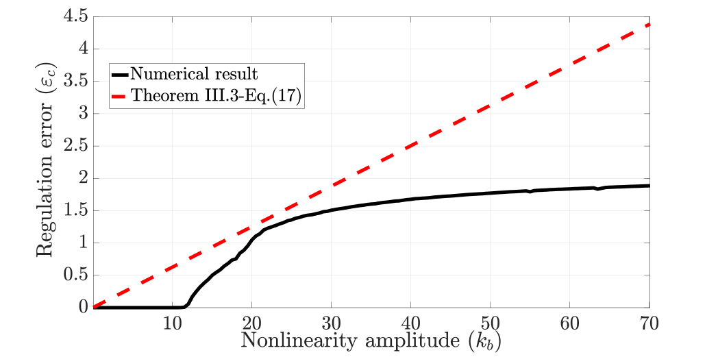
Figure 1. Impact of the nonlinearity amplitude on theoretical bound (18) in Theorem 3.3 and the actual numerical error.

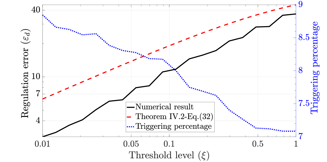
Figure 2. Impact of threshold (31) on theoretical bound (38) in Theorem 4.2, the actual numerical error, and the triggered events rate.

6. Conclusion

In this article, we introduced an optimization-based framework to synthesize robust dynamic controllers in order to ensure the output regularization task for systems with uncertain and potentially nonlinear dynamics. To numerically solve such an optimization problem, a sequential parametric convex approximate algorithm was proposed. We further introduced a general sampling-based event-triggered technique that paves the way to implement the proposed controller in case of sampled measurements and discontinuous actuation updates. It is remarkable that the procedure of the triggering law is decoupled from control synthesis and the key parameters such as maximal inter-sampling time is explicitly computationally available.

References

- [1] Cristiano M Agulhari, Ricardo CLF Oliveira, and Pedro LD Peres. relaxations for reduced-order robust control of continuous-time uncertain linear systems. IEEE Transactions on Automatic Control, 57(6):1532–1537, 2011.
- [2] Amir Ali Ahmadi and Georgina Hall. On the complexity of detecting convexity over a box. Mathematical Programming, pages 1–15, 2019.
- [3] Aharon Ben-Tal and Arkadi Nemirovski. On tractable approximations of uncertain linear matrix inequalities affected by interval uncertainty. SIAM Journal on Optimization, 12(3):811–833, 2002.
- [4] Aharon Ben-Tal, Arkadi Nemirovski, and Cornelis Roos. Extended matrix cube theorems with applications to -theory in control. Mathematics of Operations Research, 28(3):497–523, 2003.
- [5] Burak Demirel, Euhanna Ghadimi, Daniel E Quevedo, and Mikael Johansson. Optimal control of linear systems with limited control actions: threshold-based event-triggered control. IEEE Transactions on Control of Network Systems, 5(3):1275–1286, 2017.
- [6] MCF Donkers and WPMH Heemels. Output-based event-triggered control with guaranteed -gain and improved and decentralized event-triggering. IEEE Transactions on Automatic Control, 57(6):1362–1376, 2012.
- [7] John Doyle. Analysis of feedback systems with structured uncertainties. In IEE Proceedings D-Control Theory and Applications, volume 129, pages 242–250. IET, 1982.
- [8] Mahyar Fazlyab, Manfred Morari, and George J Pappas. Safety verification and robustness analysis of neural networks via quadratic constraints and semidefinite programming. IEEE Transactions on Automatic Control, 2020.
- [9] Gene F Franklin, J David Powell, Michael L Workman, et al. Digital control of dynamic systems, volume 3. Addison-wesley Menlo Park, CA, 1998.
- [10] Pascal Gahinet, Pierre Apkarian, and Mahmoud Chilali. Affine parameter-dependent lyapunov functions and real parametric uncertainty. IEEE Transactions on Automatic control, 41(3):436–442, 1996.
- [11] Bingzhao Gao, Hong Chen, Haiyan Zhao, and Kazushi Sanada. A reduced-order nonlinear clutch pressure observer for automatic transmission. IEEE Transactions on Control Systems Technology, 18(2):446–453, 2010.
- [12] WPM Heemels Heemels, MCF Donkers, and Andrew R Teel. Periodic event-triggered control for linear systems. IEEE Transactions on Automatic Control, 58(4):847–861, 2013.
- [13] Stoyan Kanev, Carsten Scherer, Michel Verhaegen, and Bart De Schutter. Robust output-feedback controller design via local BMI optimization. Automatica, 40(7):1115–1127, 2004.
- [14] Alireza Karimi, Hamid Khatibi, and Roland Longchamp. Robust control of polytopic systems by convex optimization. Automatica, 43(8):1395–1402, 2007.
- [15] Hassan K Khalil and Jessy W Grizzle. Nonlinear systems, volume 3. Prentice hall Upper Saddle River, NJ, 2002.
- [16] Gulam Dastagir Khan, Zhiyong Chen, and Lijun Zhu. A new approach for event-triggered stabilization and output regulation of nonlinear systems. IEEE Transactions on Automatic Control, 2019.
- [17] Masako Kishida, Markus Kögel, and Rolf Findeisen. Combined event-and self-triggered control approach with guaranteed finite-gain stability for uncertain linear systems. IET Control Theory & Applications, 11(11):1674–1683, 2017.
- [18] Alexander Lanzon and Ian R Petersen. Stability robustness of a feedback interconnection of systems with negative imaginary frequency response. IEEE Transactions on Automatic Control, 53(4):1042–1046, 2008.
- [19] Donghwan Lee and Jianghai Hu. A sequential parametric convex approximation method for solving bilinear matrix inequalities. In IEEE Conference on Decision and Control (CDC), pages 1965–1970, 2016.
- [20] Donghwan Lee and Jianghai Hu. Sequential parametric convex approximation algorithm for bilinear matrix inequality problem. Optimization Letters, pages 1–19, 2018.
- [21] Dong Liang and Jie Huang. Robust output regulation of linear systems by event-triggered dynamic output feedback control. IEEE Transactions on Automatic Control, 2020.
- [22] Wei Liu and Jie Huang. Event-triggered cooperative robust practical output regulation for a class of linear multi-agent systems. Automatica, 85:158–164, 2017.
- [23] Wei Liu and Jie Huang. Event-triggered global robust output regulation for a class of nonlinear systems. IEEE Transactions on Automatic Control, 62(11):5923–5930, 2017.
- [24] Wei Liu and Jie Huang. Robust practical output regulation for a class of uncertain linear minimum-phase systems by output-based event-triggered control. International Journal on Robust and Nonlinear Control, 27(18):4574–4590, 2017.
- [25] Peyman Mohajerin Esfahani and John Lygeros. A tractable fault detection and isolation approach for nonlinear systems with probabilistic performance. IEEE Transactions on Automatic Control, 61(3):633–647, 2015.
- [26] Luc Moreau and Dirk Aeyels. Practical stability and stabilization. IEEE Transactions on Automatic Control, 45(8):1554–1558, 2000.
- [27] Roberto Naldi, Michele Furci, Ricardo G Sanfelice, and Lorenzo Marconi. Robust global trajectory tracking for underactuated vtol aerial vehicles using inner-outer loop control paradigms. IEEE Transactions on Automatic Control, 62(1):97–112, 2016.
- [28] Arkadii Nemirovskii. Several -hard problems arising in robust stability analysis. Mathematics of Control, Signals and Systems, 6(2):99–105, 1993.
- [29] Tatsushi Ooba and Yasuyuki Funahashi. On a common quadratic lyapunov function for widely distant systems. IEEE Transactions on Automatic Control, 42(12):1697–1699, 1997.
- [30] Yang-Yang Qian, Lu Liu, and Gang Feng. Event-triggered robust output regulation of uncertain linear systems with unknown exosystems. IEEE Transactions on Systems, Man, and Cybernetics: Systems, 2019.
- [31] Mahdieh S Sadabadi and Dimitri Peaucelle. From static output feedback to structured robust static output feedback: A survey. Annual reviews in control, 42:11–26, 2016.
- [32] V. B. Smirnova and A. V. Proskurnikov. Volterra equations with periodic nonlinearities:multistability, oscillations and cycle slipping. Int. J. Bifurcation and Chaos, 29(5):1950068, 2019.
- [33] Paulo Tabuada. Event-triggered real-time scheduling of stabilizing control tasks. IEEE Transactions on Automatic Control, 52(9):1680–1685, 2007.
- [34] Sophie Tarbouriech, Alexandre Seuret, Christophe Prieur, and Luca Zaccarian. Insights on event-triggered control for linear systems subject to norm-bounded uncertainty. In Control Subject to Computational and Communication Constraints, pages 181–196. Springer, 2018.
- [35] Roberto Tempo, Giuseppe Calafiore, and Fabrizio Dabbene. Randomized algorithms for analysis and control of uncertain systems: with applications. Springer Science & Business Media, 2012.
- [36] Chenliang Wang, Changyun Wen, and Qinglei Hu. Event-triggered adaptive control for a class of nonlinear systems with unknown control direction and sensor faults. IEEE Transactions on Automatic Control, 65(2):763–770, 2019.
- [37] Lantao Xing, Changyun Wen, Zhitao Liu, Hongye Su, and Jianping Cai. Event-triggered output feedback control for a class of uncertain nonlinear systems. IEEE Transactions on Automatic Control, 64(1):290–297, 2019.
- [38] V.A. Yakubovich, G.A. Leonov, and A.Kh. Gelig. Stability of Stationary Sets in Control Systems with Discontinuous Nonlinearities. World Scientific Publishing Co., 2004.
- [39] Jun Yang, Jiankun Sun, Wei Xing Zheng, and Shihua Li. Periodic event-triggered robust output feedback control for nonlinear uncertain systems with time-varying disturbance. Automatica, 94:324–333, 2018.
- [40] Yuanqiang Zhou, Dewei Li, Yugeng Xi, and Zhongxue Gan. Periodic event-triggered control for distributed networked multiagents with asynchronous communication: A predictive control approach. International Journal of Robust and Nonlinear Control, 29(1):43–66, 2019.