Trajectory Poisson multi-Bernoulli filters

Abstract

This paper presents two trajectory Poisson multi-Bernoulli (TPMB) filters for multi-target tracking: one to estimate the set of alive trajectories at each time step and another to estimate the set of all trajectories, which includes alive and dead trajectories, at each time step. The filters are based on propagating a Poisson multi-Bernoulli (PMB) density on the corresponding set of trajectories through the filtering recursion. After the update step, the posterior is a PMB mixture (PMBM) so, in order to obtain a PMB density, a Kullback-Leibler divergence minimisation on an augmented space is performed. The developed filters are computationally lighter alternatives to the trajectory PMBM filters, which provide the closed-form recursion for sets of trajectories with Poisson birth model, and are shown to outperform previous multi-target tracking algorithms.

I Introduction

Multitarget tracking (MTT) consists of inferring the trajectories of an unknown number of targets that appear and disappear from a scene of interest based on noisy sensor data [1, 2]. Multitarget tracking is a fundamental process of numerous applications including advanced driver assistance systems, self-driving vehicles [3], air traffic monitoring [4] and maritime surveillance [5]. There are many approaches to perform multitarget tracking such as multiple hypothesis tracking [6, 7], joint probabilistic data association [8] and the random finite set (RFS) framework [9].

The traditional RFS approach to MTT is mainly concerned with multi-target filtering, in which one aims to estimate the current set of targets, without attempting to estimate target trajectories. In some scenarios, targets may appear anywhere in the surveillance area, while in others, targets may appear at localised areas, e.g., airports or doors. Both types of scenarios can be handled by the appropriate choice of birth model. The birth model also enables the corresponding filters to keep information on potential targets that may have been occluded [10, Fig. 6], which is key information in certain applications such as self-driving vehicles.

With Poisson point process (PPP) birth model, the solution to the multi-target filtering problem is given by the Poisson multi-Bernoulli mixture (PMBM) filter [11, 12]. If the birth model is multi-Bernoulli instead of Poisson, the filtering density is given by the multi-Bernoulli mixture (MBM) filter, which corresponds to the PMBM filtering recursion by setting the intensity of the Poisson process to zero and adding Bernoulli components for newborn targets in the prediction [12, 13]. An MBM can also be written as a mixture in which Bernoulli components have deterministic existence instead of probabilistic, giving rise to the MBM₀₁ filter [12, Sec. IV]. Deterministic existence leads to an exponential growth in the number of mixture components, which is undesirable from a computational point of view. In general, a PMBM is preferred over MBM/MBM₀₁ forms due to a more efficient representation of the information on undetected targets, via the intensity of a Poisson RFS, not limiting a priori the maximum number of new born targets at each time step [13], and being able to handle continuous-time multi-target models [14].

Even though the PMBM filter provides a closed-form solution to the multi-target filtering problem, it is also relevant to consider computationally lighter filters such as the probability hypothesis density (PHD) filter, cardinality PHD filters [9], and Poisson multi-Bernoulli (PMB) filters [11, 15]. Relations between the PMB filter and the joint integrated data association filter [16] were given in [11].

Track building procedures for the above-mentioned unlabelled filters can be obtained based on filter meta-data [17, 18, 11], i.e., information contained in the hypothesis trees. However, the posterior itself only provides information about the current set of targets, and not their trajectories. One approach to building trajectories from posterior densities is to add unique labels to the target states and form trajectories by linking target state estimates with the same label [19, 20, 21]. With labelled multi-Bernoulli birth, the $\delta$-generalised labelled multi-Bernoulli ($\delta$-GLMB) filter [20] provides the corresponding filtering density, via a recursion that is similar to the MBM₀₁ filter recursion [12, Sec. IV]. A computationally lighter alternative to the $\delta$-GLMB filter is the labelled multi-Bernoulli (LMB) filter [22]. Sequential track building approaches based on labelling can work well in many cases but it is not always adequate due to ambiguity in target-to-label associations, e.g., for independent and identically (IID) cluster birth models [23, Sec. II.B][24, Sec. III.B].

The above track building problems can be solved by computing (multi-object) densities on sets of trajectories [23], rather than sets of labelled targets. This approach has led to the following filters: trajectory PMBM (TPMBM) filter [25, 26], trajectory MBM (TMBM) filter [27], trajectory MBM₀₁ (TMBM₀₁) filter [23], and trajectory PHD (TPHD) and CPHD (TCPHD) filters [28]. These filters are analogous to their set of targets counterparts, but have the ability to estimate trajectories from first principles, and the possibility of improving the estimation of past states in the trajectories. The trajectory-based filters with multi-Bernoulli birth can be augmented to include labels, without affecting the filtering recursion [23, Sec. IV.A].

This paper proposes two trajectory PMB (TPMB) filters that approximate the trajectory PMBM filters [25] using track-oriented MBM merging [11, Sec. IV.A]. One TPMB filter aims to estimate the set of the alive trajectories at each time step, while the other aims to estimate the set of all trajectories (alive and already dead) at each time step. Keeping probabilistic information on all trajectories is important in many applications, for example, surveillance and retail analytics [29]. In the TPMB filters, the Poisson component represents information regarding trajectories that have not been detected and the multi-Bernoulli component represents information on trajectories that have been detected at some point in the past. As the true posterior is a TPMBM, the TPMB filter is derived by making use of a Kullback-Leibler divergence (KLD) minimisation, on a trajectory space with auxiliary variables, after each update, see Figure 1. The resulting TPMB density also matches the PHD of the updated TPMBM. As the TPMB filtering posterior is defined over the set of trajectories, one can estimate the set of trajectories directly from this density. In this paper, we also propose a Gaussian implementation of the TPMB filters for linear/Gaussian models. Simulation results show that the TPMB filters have a performance close to the TPMBM filters, with a decrease in computational complexity, and outperform other filters in the literature.

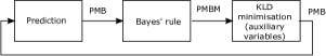
Figure 1: Diagram of the two TPMB filters. The first TPMB filter propagates a PMB density on the set of alive trajectories at the current time. After each update step, the posterior is a PMBM so the TPMB filter performs a KLD minimisation, in an augmented trajectory space with an auxiliary variable. The second TPMB filter works equivalently but propagating a PMB density on the set of all trajectories.

The rest of the paper is organised as follows. We formulate the considered multitarget tracking problems in Section II. The proposed TPMB approximation to a TPMBM density using KLD minimisation is obtained in Section III. The resulting TPMB filters are proposed in Section IV and their Gaussian implementations in Section V. Simulation results are shown in Section VI and conclusions are drawn in Section VII.

II Problem formulation

We tackle two multi-target tracking problems [25]:

1. The estimation of the set of alive trajectories at the current time step.

2. The estimation of the set of all trajectories that have existed up to the current time step. We refer to this set as the set of all trajectories.

These problems can be solved by calculating the (multi-trajectory) density over the considered set of trajectories. In this paper, we consider a computationally appealing approximation based on Poisson multi-Bernoulli densities.

II-A Set of trajectories

A single target state $x\in\mathbb{R}^{n_{x}}$ contains information of interest about the target, e.g., its position and velocity. A set of single target states $\mathbf{x}$ belongs to $\mathcal{F}\left(\mathbb{R}^{n_{x}}\right)$ where $\mathcal{F}\left(\mathbb{R}^{n_{x}}\right)$ denotes the set of all finite subsets of $\mathbb{R}^{n_{x}}$. We are interested in estimating target trajectories, where a trajectory consists of a finite sequence of target states that can start at any time step and end any time later on. A trajectory is therefore represented as a variable $X=\left(t,x^{1:\nu}\right)$ where $t$ is the initial time step of the trajectory, $\nu$ is its length and $x^{1:\nu}=\left(x^{1},...,x^{\nu}\right)$ denotes a finite sequence of length $\nu$ that contains the target states.

We consider trajectories up to the current time step $k$. As a trajectory $\left(t,x^{1:\nu}\right)$ exists from time step $t$ to $t+\nu-1$, the variable $\left(t,\nu\right)$ belongs to the set $I_{(k)}=\left\{\left(t,\nu\right):0\leq t\leq k\,\mathrm{and}\,1\leq\nu\leq k-t+1\right\}$. A single trajectory $X$ up to time step $k$ therefore belongs to the space $T_{\left(k\right)}=\uplus_{\left(t,\nu\right)\in I_{(k)}}\left\{t\right\}\times\mathbb{R}^{\nu n_{x}}$, where $\uplus$ stands for union of sets that are mutually disjoint. We denote a set of trajectories up to time step $k$ as $\mathbf{X}\in\mathcal{F}\left(T_{\left(k\right)}\right)$. Note that there can be multiple trajectories in $\mathbf{X}$ with the same $\left(t,\nu\right)$.

II-A1 Integrals and densities

Given a real-valued function $\pi\left(\cdot\right)$ on the single trajectory space $T_{\left(k\right)}$, its integral is [23]

$$\int\pi\left(X\right)dX =\sum_{\left(t,\nu\right)\in I_{(k)}}\int\pi\left(t,x^{1:\nu}\right)dx^{1:\nu}.$$ (1)

This integral goes through all possible start times, lengths and target states of the trajectory. Given a real-valued function $\pi\left(\cdot\right)$ on the space $\mathcal{F}\left(T_{\left(k\right)}\right)$ of sets of trajectories, its set integral is

$$\int\pi\left(\mathbf{X}\right)\delta\mathbf{X} =\sum_{n=0}^{\infty}\frac{1}{n!}\int\pi\left(\left\{X_{1},...,X_{n}\right\}\right)dX_{1:n}$$ (2)

where $X_{1:n}=\left(X_{1},...,X_{n}\right)$. A function $\pi\left(\cdot\right)$ is a multitrajectory density of a random finite set of trajectories if $\pi\left(\cdot\right)\geq 0$ and its set integral is one.

II-B Multi-target Bayesian models

The multi-target state evolves according to a Markov system with the following modelling:

• P1 Given the set ${\bf x}_{k}$ of targets at time step $k$, each target $x\in{\bf x}_{k}$ survives with probability $p^{S}\left(x\right)$ and moves to a new state with a transition density $g\left(\cdot\left|x\right.\right)$, or dies with probability $1-p^{S}\left(x\right)$.

• P2 The multitarget state ${\bf x}_{k+1}$ is the union of the surviving targets and new targets, where new targets are born independently following a PPP with intensity $\lambda^{B}\left(\cdot\right)$.

Set $\mathbf{x}_{k}$ is observed through the set $\mathbf{z}_{k}$ of measurements, which is modelled as

• U1 Each target state $x\in\mathbf{x}_{k}$ is either detected with probability $p^{D}\left(x\right)$ and generates one measurement with density $l\left(\cdot|x\right)$, or missed with probability $1-p^{D}\left(x\right)$.

• U2 The set $\mathbf{z}_{k}$ is the union of the target-generated measurements and Poisson clutter with intensity $\lambda^{C}\left(\cdot\right)$.

U1 and U2 imply that a measurement is generated by at most one target. The objective is to compute the posterior density of the set $\mathbf{X}_{k}$ of trajectories at time step $k$ given the sequence $\left(\mathbf{z}_{1},...,\mathbf{z}_{k}\right)$ of measurements up to time step $k$. Depending on the problem formulation, this set can correspond to the set of all trajectories or the set of alive trajectories, and the meaning will be clear from context so we use the same notation. If $\mathbf{X}_{k}$ denotes the set of alive trajectories at time step $k$, then $t+\nu-1=k$ for each $\left(t,x^{1:\nu}\right)\in\mathbf{X}_{k}$. If $\mathbf{X}_{k}$ denotes the set of all trajectories at time step $k$, then $t+\nu-1\leq k$ for each $\left(t,x^{1:\nu}\right)\in\mathbf{X}_{k}$.

II-C Poisson multi-Bernoulli mixture

Given the sequence of measurements $\left(\mathbf{z}_{1},...,\mathbf{z}_{k}\right)$ up to time step $k$ and the models in Section II-B, the density $f_{k^{\prime}|k}\left(\cdot\right)$ of the set of trajectories at time step $k^{\prime}\in\left\{k,k+1\right\}$ is a PMBM [25]. This holds for the two problem formulations we consider, though the specific recursions to compute $f_{k^{\prime}|k}\left(\cdot\right)$ vary. In both cases, $f_{k^{\prime}|k}\left(\cdot\right)$ is a PMBM with

$$f_{k^{\prime}|k}\left(\mathbf{X}_{k^{\prime}}\right) =\sum_{\mathbf{Y}\uplus\mathbf{W}=\mathbf{X}_{k^{\prime}}}f_{k^{\prime}|k}^{p}\left(\mathbf{Y}\right)f_{k^{\prime}|k}^{mbm}\left(\mathbf{W}\right)$$ (3)

$$f_{k^{\prime}|k}^{p}\left(\mathbf{X}_{k^{\prime}}\right) =e^{-\int\lambda_{k^{\prime}|k}\left(X\right)dX}\left[\lambda_{k^{\prime}|k}\left(\cdot\right)\right]^{\mathbf{X}_{k^{\prime}}}$$ (4)

$$f_{k^{\prime}|k}^{mbm}\left(\mathbf{X}_{k^{\prime}}\right) =\sum_{a\in\mathcal{A}_{k^{\prime}|k}}w_{k^{\prime}|k}^{a}\sum_{\uplus_{l=1}^{n_{k^{\prime}|k}}\mathbf{X}^{l}=\mathbf{X}_{k^{\prime}}}\prod_{i=1}^{n_{k^{\prime}|k}}f_{k^{\prime}|k}^{i,a^{i}}\left(\mathbf{X}^{i}\right)$$ (5)

where the sum in (3) goes through all disjoint and possibly empty sets $\mathbf{Y}$ and $\mathbf{W}$ such that $\mathbf{Y}\cup\mathbf{W}=\mathbf{X}_{k^{\prime}}$, the multi-object exponential is defined as $h^{\mathbf{X}}=\prod_{X\in\mathbf{X}}h\left(X\right)$ where $h$ is a real-valued function and $h^{\emptyset}=1$ by convention, and

$$f_{k^{\prime}|k}^{i,a^{i}}\left(\mathbf{X}\right) =\begin{cases}1-r_{k^{\prime}|k}^{i,a^{i}}&\mathbf{X}=\emptyset\\ r_{k^{\prime}|k}^{i,a^{i}}p_{k^{\prime}|k}^{i,a^{i}}\left(X\right)&\mathbf{X}=\left\{X\right\}\\ 0&\mathrm{otherwise}.\end{cases}$$ (6)

We proceed to explain the aspects of (3) that are relevant to our contribution; for details, we refer the reader to [25, 11].

From (3), the PMBM is the union of two independent RFS: a Poisson RFS with (multi-trajectory) density $f_{k^{\prime}|k}^{p}\left(\cdot\right)$ that represents undetected trajectories, and a mixture of multi-Bernoulli RFS $f_{k^{\prime}|k}^{mbm}\left(\cdot\right)$ that represents trajectories that have been detected at some point up to time step $k$. The Poisson RFS on undetected targets/trajectories provides very valuable information in some applications. For example, in self-driving vehicles the Poisson RFS can indicate areas where there may be pedestrians or vehicles that have not been yet detected by our sensors [10]. The intensity of the Poisson RFS is denoted as $\lambda_{k^{\prime}|k}\left(\cdot\right)$. Each received measurement generates a unique Bernoulli component. The number of Bernoulli components is $n_{k^{\prime}|k}$, and they are indexed by variable $i$. A global hypothesis is $a=\left(a^{1},...,a^{n_{k^{\prime}|k}}\right)$, where $a^{i}\in\left\{1,...,h^{i}\right\}$ is the index to the local hypothesis for the $i$-th Bernoulli and $h^{i}$ is the number of local hypotheses. The weight of global hypothesis $a$ is

$$w_{k^{\prime}|k}^{a} =\frac{\prod_{i=1}^{n_{k^{\prime}|k}}w_{k^{\prime}|k}^{i,a^{i}}}{\sum_{b\in\mathcal{A}_{k^{\prime}|k}}\prod_{i=1}^{n_{k^{\prime}|k}}w_{k^{\prime}|k}^{i,b^{i}}}$$ (7)

where $w_{k^{\prime}|k}^{i,a^{i}}$ is the weight of local hypothesis $a_{i}$ for Bernoulli $i$. The set $\mathcal{A}_{k^{\prime}|k}$ contains all global hypotheses [11]. The density of the $i$-th Bernoulli with local hypothesis $a^{i}$ is $f_{k^{\prime}|k}^{i,a^{i}}\left(\cdot\right)$, with probability $r_{k^{\prime}|k}^{i,a^{i}}$ of existence and single-trajectory density $p_{k^{\prime}|k}^{i,a^{i}}\left(\cdot\right)$. We can also write (3) as

$$f_{k^{\prime}|k}\left(\mathbf{X}_{k^{\prime}}\right)$$

$$=\sum_{\uplus_{l=1}^{n_{k^{\prime}|k}}\mathbf{X}^{l}\uplus\mathbf{Y}=\mathbf{X}_{k^{\prime}}}f_{k^{\prime}|k}^{p}\left(\mathbf{Y}\right)\sum_{a\in\mathcal{A}_{k^{\prime}|k}}w_{k^{\prime}|k}^{a}\prod_{i=1}^{n_{k^{\prime}|k}}\left[f_{k^{\prime}|k}^{i,a^{i}}\left(\mathbf{X}^{i}\right)\right].$$ (8)

We will use this formulation in Section III-A, where we introduce auxiliary variables.

III Trajectory PMB approximation

In this section we first introduce auxiliary variables in the PMBM (8) in Section III-A. Then, we provide the best PMB approximation to the PMBM with auxiliary variables, in the sense of minimising the resulting KLD in Section III-B. Finally, in Section III-C, we show the relation between the KLDs with and without auxiliary variables.

III-A PMBM with auxiliary variables

In this section, we introduce an auxiliary variable in the PMBM representation in (8) that will be useful to obtain the PMB approximation. Auxiliary variables are commonly used in Bayesian inference to deal with mixtures of densities, especially in sampling-based methods [30, 31, 19, 32, 33, 34, 35, 36] and latent variable models, e.g., expectation-maximisation [37]. Given (8), we extend the single trajectory space with an auxiliary variable $u\in\mathbb{\mathbb{U}}_{k^{\prime}|k}=\left\{0,1,..,n_{k^{\prime}|k}\right\}$, such that $\left(u,X\right)\in\mathbb{\mathbb{U}}_{k^{\prime}|k}\times T_{\left(k^{\prime}\right)}$. As will become clearer at the end of this section, variable $u=0$ implies that the single trajectory has not yet been detected, so it corresponds to the PPP, and $u=i$ indicates that the single trajectory corresponds to the $i$-th Bernoulli component. We denote a set of trajectories with auxiliary variables as $\widetilde{\mathbf{X}}_{k^{\prime}}\in\mathcal{F}\left(\mathbb{\mathbb{U}}_{k^{\prime}|k}\times T_{\left(k^{\prime}\right)}\right)$.

Definition 1.

Given $f_{k^{\prime}|k}\left(\cdot\right)$ of the form (8), we define the density $\widetilde{f}_{k^{\prime}|k}\left(\cdot\right)$ on the space $\mathcal{F}\left(\mathbb{\mathbb{U}}_{k^{\prime}|k}\times T_{\left(k^{\prime}\right)}\right)$ of sets of trajectories with auxiliary variable as

$$\widetilde{f}_{k^{\prime}|k}\left(\widetilde{\mathbf{X}}_{k^{\prime}}\right)$$

$$=\sum_{\uplus_{l=1}^{n_{k^{\prime}|k}}\mathbf{\widetilde{X}}^{l}\uplus\widetilde{\mathbf{Y}}=\widetilde{\mathbf{X}}_{k^{\prime}}}\widetilde{f}_{k^{\prime}|k}^{p}\left(\widetilde{\mathbf{Y}}\right)\sum_{a\in\mathcal{A}_{k^{\prime}|k}}w_{k^{\prime}|k}^{a}\prod_{i=1}^{n_{k^{\prime}|k}}\left[\widetilde{f}_{k^{\prime}|k}^{i,a^{i}}\left(\mathbf{\widetilde{X}}^{i}\right)\right]$$

$$=\widetilde{f}_{k^{\prime}|k}^{p}\left(\widetilde{\mathbf{Y}}_{k^{\prime}}\right)\sum_{a\in\mathcal{A}_{k^{\prime}|k}}w_{k^{\prime}|k}^{a}\prod_{i=1}^{n_{k^{\prime}|k}}\left[\widetilde{f}_{k^{\prime}|k}^{i,a^{i}}\left(\widetilde{\mathbf{X}}_{k^{\prime}}^{i}\right)\right]$$ (9)

where, for a given $\widetilde{\mathbf{X}}_{k^{\prime}}$, $\widetilde{\mathbf{Y}}_{k^{\prime}}=\left\{\left(u,X\right)\in\widetilde{\mathbf{X}}_{k^{\prime}}:u=0\right\}$ and $\widetilde{\mathbf{X}}_{k^{\prime}}^{i}=\left\{\left(u,X\right)\in\widetilde{\mathbf{X}}_{k^{\prime}}:u=i\right\}$, and

$$\widetilde{f}_{k^{\prime}|k}^{p}\left(\widetilde{\mathbf{X}}\right) =e^{-\int\lambda_{k^{\prime}|k}\left(x\right)dx}\left[\widetilde{\lambda}_{k^{\prime}|k}\left(\cdot\right)\right]^{\widetilde{\mathbf{X}}}$$ (10)

$$\widetilde{\lambda}_{k^{\prime}|k}\left(u,X\right) =\delta_{0}\left[u\right]\lambda_{k^{\prime}|k}\left(X\right)$$ (11)

$$\widetilde{f}_{k^{\prime}|k}^{i,a^{i}}\left(\widetilde{\mathbf{X}}\right) =\begin{cases}1-r_{k^{\prime}|k}^{i,a^{i}}&\widetilde{\mathbf{X}}=\emptyset\\ r_{k^{\prime}|k}^{i,a^{i}}p_{k^{\prime}|k}^{i,a^{i}}\left(X\right)\delta_{i}\left[u\right]&\widetilde{\mathbf{X}}=\left\{\left(u,X\right)\right\}\\ 0&\mathrm{otherwise}\end{cases}$$ (12)

where the Kronecker delta $\delta_{i}\left[u\right]=1$ if $u=i$ and $\delta_{i}\left[u\right]=0$, otherwise. Note that the sum over sets disappears in (9) as there is only one possible partition of $\widetilde{\mathbf{X}}_{k^{\prime}}$ into $\widetilde{\mathbf{Y}},$ $\mathbf{\widetilde{X}}^{1}$,…, $\mathbf{\widetilde{X}}^{n_{k^{\prime}|k}}$ that provides a non-zero density. In addition, if two or more trajectories in $\widetilde{\mathbf{X}}_{k^{\prime}}$ have non-zero auxiliary variables that are equal, then $\widetilde{f}_{k^{\prime}|k}\left(\widetilde{\mathbf{X}}_{k^{\prime}}\right)=0$, as the corresponding Bernoulli component (12) evaluated for more than one trajectory is zero. Conversely, there can be multiple trajectories in $\widetilde{\mathbf{X}}_{k^{\prime}}$ whose auxiliary variable is zero, without implying that $\widetilde{f}_{k^{\prime}|k}\left(\widetilde{\mathbf{X}}_{k^{\prime}}\right)=0$. Also, the density $\widetilde{f}_{k^{\prime}|k}\left(\cdot\right)$ has domain $\mathcal{F}\left(\mathbb{\mathbb{U}}_{k^{\prime}|k}\times T_{\left(k^{\prime}\right)}\right)$ which implies that we only consider auxiliary variables $u\in\mathbb{\mathbb{U}}_{k^{\prime}|k}=\left\{0,1,..,n_{k^{\prime}|k}\right\}$.

The definition of $\widetilde{f}_{k^{\prime}|k}\left(\cdot\right)$ is mathematically sound as it defines a density in $\mathcal{F}\left(\mathbb{\mathbb{U}}_{k^{\prime}|k}\times T_{\left(k^{\prime}\right)}\right)$ and, as we prove in App. A, integrating out the auxiliary variables, we recover the original density. This procedure of introducing auxiliary variables for PMBM for sets of trajectories is also directly applicable for PMBM for sets of targets. In the target case, the proposed use of auxiliary variables bears resemblance to the approaches in [5, Sec. IX][38, 39], in which targets that have never been detected are indistinguishable, in our case represented by the PPP with $u=0$, and targets that have been detected are distinguishable, in our case represented by a unique $u>0$ and a Bernoulli density. Therefore, $u$ can be considered a mark [40], but it is not a label, as in a labelled approach [20], each target must have a unique label.

III-B KLD minimisation with auxiliary variables

In this section, we derive the best PMB fit of a PMBM using KLD minimisation on the space with auxiliary variables.

III-B1 Kullback-Leibler divergence

Given a real-valued function $\pi\left(\cdot\right)$ on the single trajectory space $\mathbb{\mathbb{U}}_{k^{\prime}|k}\times T_{\left(k^{\prime}\right)}$ with auxiliary variable, its single-trajectory integral is

$$\int\pi\left(\widetilde{X}\right)d\widetilde{X} =\sum_{u\in\mathbb{\mathbb{U}}_{k^{\prime}|k}}\sum_{\left(t,\nu\right)\in I_{(k^{\prime})}}\int\pi\left(u,t,x^{1:\nu}\right)dx^{1:\nu}.$$ (13)

Given two densities $\widetilde{f}\left(\cdot\right)$ and $\widetilde{q}\left(\cdot\right)$ on the space $\mathcal{F}\left(\mathbb{\mathbb{U}}_{k^{\prime}|k}\times T_{\left(k^{\prime}\right)}\right)$ of sets of trajectories with auxiliary variable, the KLD $\mathrm{D}\left(\widetilde{f}\left\|\widetilde{q}\right.\right)$ is

$$\mathrm{D}\left(\widetilde{f}\left\|\widetilde{q}\right.\right) =\int\widetilde{f}\left(\widetilde{\mathbf{X}}\right)\log\frac{\widetilde{f}\left(\widetilde{\mathbf{X}}\right)}{\widetilde{q}\left(\widetilde{\mathbf{X}}\right)}\delta\widetilde{\mathbf{X}}.$$ (14)

III-B2 PMB approximation

We aim to obtain a PMB approximation $\widetilde{q}\left(\cdot\right)$ on the space $\mathcal{F}\left(\mathbb{\mathbb{U}}_{k^{\prime}|k}\times T_{\left(k^{\prime}\right)}\right)$ such that

$$\widetilde{q}\left(\widetilde{\mathbf{X}}_{k^{\prime}}\right) =\widetilde{q}^{p}\left(\widetilde{\mathbf{Y}}_{k^{\prime}}\right)\prod_{i=1}^{n_{k^{\prime}|k}}\left[\widetilde{q}^{i,1}\left(\widetilde{\mathbf{X}}_{k^{\prime}}^{i}\right)\right]$$ (15)

where $\widetilde{q}^{p}\left(\cdot\right)$ is of the form (10) with intensity $\lambda^{q}\left(\cdot\right)$ and $\widetilde{q}^{i,1}\left(\cdot\right)$ is of the form (12) with existence probability $r^{i}$ and single-trajectory density $p^{i}\left(\cdot\right)$.

Proposition 2.

Given a PMBM density $\widetilde{f}_{k^{\prime}|k}\left(\cdot\right)$ of the form (9), the parameters of the PMB density $\widetilde{q}\left(\cdot\right)$, see (15), that minimises the KLD $\mathrm{D}\left(\widetilde{f}_{k^{\prime}|k}\left\|\widetilde{q}\right.\right)$ are given by

$$\lambda^{q}\left(X\right) =\lambda_{k^{\prime}|k}\left(X\right)$$ (16)

$$r^{i} =\sum_{a^{i}=1}^{h^{i}}\overline{w}_{k^{\prime}|k}^{i,a^{i}}r_{k^{\prime}|k}^{i,a^{i}}$$ (17)

$$p^{i}\left(X\right) =\frac{\sum_{a^{i}=1}^{h^{i}}\overline{w}_{k^{\prime}|k}^{i,a^{i}}r_{k^{\prime}|k}^{i,a^{i}}p_{k^{\prime}|k}^{i,a^{i}}\left(X\right)}{\sum_{a^{i}=1}^{h^{i}}\overline{w}_{k^{\prime}|k}^{i,a^{i}}r_{k^{\prime}|k}^{i,a^{i}}}$$ (18)

where

$$\overline{w}_{k^{\prime}|k}^{i,a^{i}} =\sum_{b\in\mathcal{A}_{k^{\prime}|k}:b^{i}=a^{i}}w_{k^{\prime}|k}^{b}.$$ (19)

Proposition 2 is proved in App. B. Note that we can also write $r^{i}$ and $p^{i}\left(\cdot\right)$ as in (92) and (93). Nevertheless, (17) and (18) are more suitable for implementation than (92) and (93), as the sum for $p^{i}\left(\cdot\right)$ in (18) has a single term for each $p_{k^{\prime}|k}^{i,a^{i}}\left(\cdot\right)$. In App. B, we also show that the PHD of $\widetilde{q}\left(\cdot\right)$ matches the PHD of $\widetilde{f}_{k^{\prime}|k}\left(\cdot\right)$.

III-C Relation between KLDs

In this section, we establish that the KLD on the space of sets of trajectories with auxiliary variables is an upper bound on the KLD for sets of trajectories without auxiliary variables.

Lemma 3.

Let $f_{k^{\prime}|k}\left(\cdot\right)$ and $\widetilde{f}{}_{k^{\prime}|k}\left(\cdot\right)$ be the PMBMs in (8) and (9). Let $q\left(\cdot\right)$ denote a multi-trajectory density and $\widetilde{q}\left(\cdot\right)$ an extension of $q\left(\cdot\right)$ with auxiliary variables. Then,

$$\mathrm{D}\left(f_{k^{\prime}|k}\left\|q\right.\right) \leq\mathrm{D}\left(\widetilde{f}{}_{k^{\prime}|k}\left\|\widetilde{q}\right.\right).$$ (20)

The proof of Lemma 3 is given in App. B. The KLD $\mathrm{D}\left(f_{k^{\prime}|k}\left\|q\right.\right)$ is the one we are primarily interested in, as it does not include auxiliary variables. Nevertheless, introducing auxiliary variables enables us to minimise the resulting KLD in closed-form, which is an upper bound on $\mathrm{D}\left(f_{k^{\prime}|k}\left\|q\right.\right)$.

IV Trajectory PMB filters

In Section IV-A, we explain the dynamic and measurement models written for sets of alive trajectories and sets of all trajectories. The filtering recursions of the TPMB filters are provided in Section IV-B.

IV-A Bayesian models for sets of trajectories

We proceed to write the Bayesian dynamic/measurement models for the two types of problem formulations [25]. These models are required for the filtering recursions in Section IV-B. In particular, we specify the intensity $\lambda_{k+1}^{B}\left(X\right)$ of new born trajectories, the single trajectory transition density $g_{k+1}\left(\cdot\left|X\right.\right)$ and the probability $p^{S}\left(X\right)$ of survival as a function of a trajectory $X$. In this paper, $p^{S}\left(X\right)$ refers to the probability that a trajectory remains in the considered set of trajectories (either all trajectories or alive trajectories) and is different from $p^{S}\left(x\right)$ as a function on a target state $x$.

IV-A1 Dynamic model for the set of alive trajectories

The set of alive trajectories evolves according to this Markov system

• P1T Given the set ${\bf X}_{k}$ of alive trajectories at time step $k$, each $X=\left(t,x^{1:\nu}\right)\in{\bf X}_{k}$, where $t+\nu-1=k$, either survives with probability $p^{S}\left(X\right)=p^{S}\left(x^{\nu}\right)$ with a transition density

  $$g_{k+1}\left(t_{y},y{}^{1:\nu_{y}}\left|X\right.\right) =\delta_{t}\left[t_{y}\right]\delta_{\nu+1}\left[\nu_{y}\right]\delta_{x^{1:\nu}}\left(y^{1:\nu_{y}-1}\right)$$

  $$\,\times g\left(y^{\nu_{y}}\left|x^{\nu}\right.\right)$$ (21)

  or dies with probability $1-p^{S}\left(X\right)$.

• P2T The set ${\bf X}_{k+1}$ is the union of the surviving trajectories and new trajectories, which are born independently following a PPP with intensity

  $$\lambda_{k+1}^{B}\left(t,x^{1:\nu}\right) =\delta_{k+1}\left[t\right]\delta_{1}\left[\nu\right]\lambda^{B}\left(x^{\nu}\right).$$ (22)

IV-A2 Dynamic model for the set of all trajectories

The set of all trajectories evolves according to this Markov system

• P3T Given the set ${\bf X}_{k}$ of all trajectories at time step $k$, each $X=\left(t,x^{1:\nu}\right)\in{\bf X}_{k}$, where $t+\nu-1\leq k$, survives with probability 1, $p^{S}\left(X\right)=1$, with a transition density

  $$g_{k+1}\left(t_{y},y{}^{1:\nu_{y}}\left|X\right.\right)=\delta_{t}\left[t_{y}\right]$$

  $$\times\begin{cases}\delta_{\nu}\left[\nu_{y}\right]\delta_{x^{1:\nu}}\left(y^{1:\nu_{y}}\right)&\omega_{y}<k\\ \delta_{\nu}\left[\nu_{y}\right]\delta_{x^{1:\nu}}\left(y^{1:\nu_{y}}\right)\left(1-p^{S}\left(x^{\nu}\right)\right)&\omega_{y}=k\\ \delta_{\nu+1}\left[\nu_{y}\right]\delta_{x^{1:\nu}}\left(y^{1:\nu_{y}-1}\right)p^{S}\left(x^{\nu}\right)\\ \quad\times g\left(y^{\nu_{y}}\left|x^{\nu}\right.\right)&\omega_{y}=k+1\end{cases}$$

  where $\omega_{y}=t_{y}+\nu_{y}-1$.

• Same birth model as in P2T.

It should be noted that $g_{k+1}\left(\cdot\right)$ does not depend on $k$ in P1T (alive trajectories) but it depends on $k$ in P3T (all trajectories). Nevertheless, we write the dependence on $k$ in both settings to have a unified notation for both transition densities.

IV-A3 Measurement model for sets of trajectories

The measurement model U1 and U2 can be written for sets of all trajectories and sets of alive trajectories in the same manner:

• U1T Each trajectory $\left(t,x^{1:\nu}\right)\in\mathbf{X}_{k}$, where $\mathbf{X}_{k}$ is the set of (all or alive) trajectories, is detected with probability

  $$p_{k}^{D}\left(t,x^{1:\nu}\right) =\begin{cases}p^{D}\left(x^{\nu}\right)&t+\nu-1=k\\ 0&\mathrm{otherwise}\end{cases}$$ (23)

  and generates one measurement with density $l\left(\cdot|t,x^{1:\nu}\right)=l\left(\cdot|x^{\nu}\right)$ or misdetected with probability $1-p_{k}^{D}\left(t,x^{1:\nu}\right)$.

• Same clutter model as in U2.

IV-B Filtering recursions

We present the prediction and update in Sections IV-B1 and IV-B2. Given two real-valued functions $a\left(\cdot\right)$ and $b\left(\cdot\right)$ on the single-trajectory space, we denote

$$\left\langle a,b\right\rangle =\int a\left(X\right)b\left(X\right)dX.$$ (24)

IV-B1 Prediction

We denote the PMB filtering/predicted densities over the set of trajectories at time step $k$, with $k^{\prime}\in\left\{k,k+1\right\}$, as

$$f_{k^{\prime}|k}\left(\mathbf{X}_{k^{\prime}}\right) =\sum_{\uplus_{l=1}^{n_{k^{\prime}|k}}\mathbf{X}^{l}\uplus\mathbf{Y}=\mathbf{X}_{k^{\prime}}}f_{k^{\prime}|k}^{p}\left(\mathbf{Y}\right)\prod_{i=1}^{n_{k^{\prime}|k}}\left[f_{k^{\prime}|k}^{i}\left(\mathbf{X}^{i}\right)\right]$$ (25)

where the intensity of the Poisson component is $\lambda_{k^{\prime}|k}\left(\cdot\right)$, $n_{k^{\prime}|k}$ is the number of Bernoulli components and the probability of existence and single target density of the $i$-th Bernoulli component are $r_{k^{\prime}|k}^{i}$ and $p_{k^{\prime}|k}^{i}\left(\cdot\right)$.

Lemma 4 (TPMB prediction).

Given the PMB filtering density on the set of trajectories at time step $k-1$ of the form (25), the predicted density at time step $k$ is a PMB of the form (25), with $n_{k|k-1}=n_{k-1|k-1}$ and

$$\lambda_{k|k-1}\left(X\right) =\lambda_{k}^{B}\left(X\right)+\left\langle\lambda_{k-1|k-1},g_{k}\left(X|\cdot\right)p^{S}\left(\cdot\right)\right\rangle$$ (26)

$$r_{k|k-1}^{i} =r_{k-1|k-1}^{i}\left\langle p_{k-1|k-1}^{i},p^{S}\right\rangle$$ (27)

$$p_{k|k-1}^{i}\left(X\right) =\frac{\left\langle p_{k-1|k-1}^{i},g_{k}\left(X|\cdot\right)p^{S}\left(\cdot\right)\right\rangle}{\left\langle p_{k-1|k-1}^{i},p^{S}\right\rangle}$$ (28)

where $g_{k}\left(\cdot|\cdot\right)$, $p^{S}\left(\cdot\right)$ and $\lambda_{B,k}\left(\cdot\right)$ are chosen depending on the problem formulation: for alive trajectories, see Section IV-A1, and for all trajectories, see Section IV-A2.

Lemma 4 is a particular case of the TPMBM predictor [25], as a PMB is a PMBM with only one mixture component.

IV-B2 Update

The update of the TPMB filter is obtained by first doing a Bayesian update, which yields a PMBM distribution, followed by a KLD minimisation, on the space with auxiliary variables, as was illustrated in Figure 1.

Lemma 5 (TPMB update).

Given the PMB predicted density on the set of trajectories at time step $k$ of the form (25), and a measurement set $\mathbf{z}_{k}=\left\{z_{k}^{1},...,z_{k}^{m_{k}}\right\}$, the updated distribution is a PMBM of the form (3) where $n_{k|k}=n_{k|k-1}+m_{k}$ and

$$\lambda_{k|k}\left(X\right) =\left(1-p_{k}^{D}\left(X\right)\right)\lambda_{k|k-1}\left(X\right).$$ (29)

For each Bernoulli component in $f_{k|k-1}\left(\cdot\right)$, $i\in\left\{1,...,n_{k|k-1}\right\}$, there are $h^{i}=m_{k}+1$ local hypotheses, corresponding to a misdetection and an update with one of the measurements. The misdetection hypothesis for Bernoulli component $i\in\left\{1,...,n_{k|k-1}\right\}$ is given by $\mathcal{M}\left(i,1\right)=\emptyset$,

$$w_{k|k}^{i,1} =1-r_{k|k-1}^{i}\left\langle p_{k|k-1}^{i},p_{k}^{D}\right\rangle$$ (30)

$$r_{k|k}^{i,1} =\frac{r_{k|k-1}^{i}\left\langle p_{k|k-1}^{i},1-p_{k}^{D}\right\rangle}{1-r_{k|k-1}^{i}\left\langle p_{k|k-1}^{i},p_{k}^{D}\right\rangle}$$ (31)

$$p_{k|k}^{i,1}\left(X\right) =\frac{\left(1-p_{k}^{D}\left(X\right)\right)p_{k|k-1}^{i}\left(X\right)}{\left\langle p_{k|k-1}^{i},1-p_{k}^{D}\right\rangle}.$$ (32)

The hypothesis for Bernoulli component $i\in\left\{1,...,n_{k|k-1}\right\}$ and measurement $z_{k}^{j}$ is given by $\mathcal{M}\left(i,j\right)=\left\{j\right\}$, $r_{k|k}^{i,1+j}=1$,

$$w_{k|k}^{i,1+j} =r_{k|k-1}^{i}\left\langle p_{k|k-1}^{i},l\left(z_{k}^{j}|\cdot\right)p_{k}^{D}\left(\cdot\right)\right\rangle$$ (33)

$$p_{k|k}^{i,1+j}\left(X\right) =\frac{l\left(z_{k}^{j}|X\right)p_{k}^{D}\left(X\right)p_{k|k-1}^{i}\left(X\right)}{\left\langle p_{k|k-1}^{i},l\left(z_{k}^{j}|\cdot\right)p_{k}^{D}\left(\cdot\right)\right\rangle}.$$ (34)

For a new Bernoulli component $i\in\left\{n_{k|k-1}+j\right\}$, $j\in\left\{1,...,m_{k}\right\}$, which is initiated by measurement $z_{k}^{j}$, there are $h_{i}=2$ local hypotheses

$$\mathcal{M}\left(i,1\right)=\emptyset,\,w_{k|k}^{i,1}=1,\,r_{k|k}^{i,1}=0,\>\mathcal{M}\left(i,2\right)=\left\{j\right\}$$ (35)

$$w_{k|k}^{i,2} =\lambda^{C}\left(z_{k}^{j}\right)+\left\langle\lambda_{k|k-1},l\left(z_{k}^{j}|\cdot\right)p_{k}^{D}\left(\cdot\right)\right\rangle$$ (36)

$$r_{k|k}^{i,2} =\frac{\left\langle\lambda_{k|k-1},l\left(z_{k}^{j}|\cdot\right)p_{k}^{D}\left(\cdot\right)\right\rangle}{\lambda^{C}\left(z_{k}^{j}\right)+\left\langle\lambda_{k|k-1},l\left(z_{k}^{j}|\cdot\right)p_{k}^{D}\left(\cdot\right)\right\rangle}$$ (37)

$$p_{k|k}^{i,2}\left(X\right) =\frac{l\left(z_{k}^{j}|X\right)p_{k}^{D}\left(X\right)\lambda_{k|k-1}\left(X\right)}{\left\langle\lambda_{k|k-1},l\left(z_{k}^{j}|\cdot\right)p_{k}^{D}\left(\cdot\right)\right\rangle}.$$ (38)

The set $\mathcal{M}\left(i,j\right)$ indicates the measurement index for Bernoulli component $i$ and local hypothesis $j$. The set of global data association hypotheses is

$$\mathcal{A}_{k} =\left\{\vphantom{\bigcup_{i=1}^{n_{k|k}}}\left(a_{1},...,a_{n_{k|k}}\right):a_{i}\in\mathbb{N}_{h_{i}},\bigcup_{i=1}^{n_{k|k}}\mathcal{M}\left(i,a_{i}\right)=\mathbb{N}_{m_{k}},\right.$$

$$\left.\quad\mathcal{M}\left(i,a_{i}\right)\cap\mathcal{M}\left(j,a_{j}\right)=\emptyset\,\forall i\neq j\vphantom{\bigcup_{i=1}^{n_{k|k}}}\right\}$$ (39)

where $\mathbb{N}_{m_{k}}=\left\{1,...,m_{k}\right\}$.

Lemma 5 is the same for both problem formulations and corresponds to the TPMBM update [25] when the predicted density is a PMB. Finally, the projection of this PMBM density to a PMB density is obtained by Proposition 2.

The results in Lemma 4 and 5 are conceptually analogous to the PMBM recursion for targets [11, 12]. However, these lemmas operate on sets of trajectories, which requires using single trajectory densities and integrals, and establishing the corresponding $p^{S}\left(\cdot\right)$, $g_{k+1}\left(\cdot\left|X\right.\right)$ and $\lambda_{k+1}^{B}\left(\cdot\right)$ depending on the problem formulation, see Section IV-A. Also, the set of global hypotheses (39) is different from the global hypotheses of the PMBM recursion on sets of targets [11, 12], as it considers a PMB prior, not a PMBM prior.

V Gaussian TPMB filters

In this section, we explain the Gaussian implementation of the TPMB filter for alive trajectories and all trajectories in Section V-A and V-B, respectively. Practical considerations are provided in Section V-C. Trajectory estimation is explained in Section V-D. Finally, a discussion is provided in Section V-E.

We use the notation

$$\mathcal{N}\left(t,x^{1:\nu};\tau,\overline{x},P\right) =\begin{cases}\mathcal{N}\left(x^{1:\nu};\overline{x},P\right)&t=\tau,\,\nu=\iota\\ 0&\mathrm{otherwise}\end{cases}$$ (40)

where $\iota=\mathrm{dim}\left(\overline{x}\right)/n_{x}$. Equation (40) represents a single trajectory Gaussian density with start time $\tau$, duration $\iota$, mean $\overline{x}\in\mathbb{R}^{\iota n_{x}}$ and covariance matrix $P\in\mathbb{R}^{\iota n_{x}\times\iota n_{x}}$ evaluated at $\left(t,x^{1:\nu}\right)$. We use $\otimes$ to indicate the Kronecker product and $0_{m,n}$ is the $m\times n$ zero matrix.

We make the additional assumptions

• A1 The survival and detection probabilities are constants: $p^{S}\left(x\right)=p^{S}$ and $p^{D}\left(x\right)=p^{D}$, see P1 and U1.

• A2 $g\left(\cdot\left|x\right.\right)=\mathcal{N}\left(\cdot;Fx,Q\right)$ and $l\left(\cdot|x\right)=\mathcal{N}\left(\cdot;Hx,R\right)$.

• A3 The PHD of the birth density at time step $k$ is

  $$\lambda_{k}^{B}\left(X\right) =\sum_{q=1}^{n_{k}^{b}}w_{k}^{b,q}\mathcal{N}\left(X;k,\overline{x}_{k}^{b,q},P_{k}^{b,q}\right)$$ (41)

  where $n_{k}^{b}\in\mathbb{N}$ is the number of components, $w_{k}^{b,q}$ is the weight of the $q$th component, $\overline{x}_{k}^{b,q}\in\mathbb{R}^{n_{x}}$ its mean and $P_{k}^{b,q}\in\mathbb{R}^{n_{x}\times n_{x}}$ its covariance matrix.

V-A Gaussian implementation for alive trajectories

In the Gaussian implementation for alive trajectories, the single-trajectory density of the $i$-th Bernoulli component, see (25), is of the form

$$p_{k^{\prime}|k}^{i}\left(X\right) =\mathcal{N}\left(X;t^{i},\overline{x}_{k^{\prime}|k}^{i},P_{k^{\prime}|k}^{i}\right)$$ (42)

where $t^{i}$ is the start time, $\overline{x}_{k^{\prime}|k}^{i}$ is the mean, $P_{k^{\prime}|k}^{i}$ the covariance matrix and $t^{i}+\mathrm{dim}\left(\overline{x}_{k^{\prime}|k}^{i}\right)/n_{x}-1=k^{\prime}$, which implies that the trajectory is alive at time step $k^{\prime}$,

The PPP has a Gaussian mixture intensity

$$\lambda_{k^{\prime}|k}\left(X\right) =\sum_{q=1}^{n_{k^{\prime}|k}^{p}}w_{k^{\prime}|k}^{p,q}\mathcal{N}\left(X;t_{k^{\prime}|k}^{p,q},\overline{x}_{k^{\prime}|k}^{p,q},P_{k^{\prime}|k}^{p,q}\right)$$ (43)

where $n_{k^{\prime}|k}^{p}$ is the number of components, $w_{k^{\prime}|k}^{p,q}$ is the weight of the $q$th component, $t_{k^{\prime}|k}^{p,q}$ is starting time, $\overline{x}_{k^{\prime}|k}^{p,q}$ its mean and $P_{k^{\prime}|k}^{p,q}$ its covariance matrix.

The prediction step is given by the following lemma.

Lemma 6 (GTPMB prediction, alive trajectories).

Assume the filtering density for the alive trajectories is a PMB (25) with $p_{k-1|k-1}^{i}\left(\cdot\right)$ and $\lambda_{k-1|k-1}\left(\cdot\right)$ given by (42) and (43). Then, the predicted density is a PMB of the form (25) with

$$r_{k|k-1}^{i} =p^{S}r_{k-1|k-1}^{i}$$ (44)

$$\overline{x}_{k|k-1}^{i} =\left[\left(\overline{x}_{k-1|k-1}^{i}\right)^{T},\left(\overline{F}_{i}\overline{x}_{k-1|k-1}^{i}\right)^{T}\right]^{T}$$ (45)

$$P_{k|k-1}^{i} =\left[\begin{array}[]{cc}P_{k-1|k-1}^{i}&P_{k-1|k-1}^{i}\overline{F}_{i}^{T}\\ \overline{F}_{i}P_{k-1|k-1}^{i}&\overline{F}_{i}P_{k-1|k-1}^{i}\overline{F}_{i}^{T}+Q\end{array}\right]$$ (48)

$$\overline{F}_{i} =\left[0_{1,\iota^{i}-1},1\right]\otimes F,$$ (49)

$$\lambda_{k|k-1}\left(X\right) =\sum_{q=1}^{n_{k}^{b}}w_{k}^{b,q}\mathcal{N}\left(X;k,\overline{x}_{k}^{b,q},P_{k}^{b,q}\right)+p^{S}\sum_{q=1}^{n_{k-1|k-1}^{p}}$$

$$\,w_{k-1|k-1}^{p,q}\mathcal{N}\left(X;t_{k-1|k-1}^{p,q},\overline{x}_{k|k-1}^{p,q},P_{k|k-1}^{p,q}\right)$$ (50)

where $\iota^{i}=\mathrm{dim}\left(\overline{x}_{k-1|k-1}^{i}\right)/n_{x}$ and $\overline{x}_{k|k-1}^{p,q}$ and $P_{k|k-1}^{p,q}$ are obtained by (45) and (48) using $\overline{x}_{k-1|k-1}^{p,q}$ and $P_{k-1|k-1}^{p,q}$ instead of $\overline{x}_{k-1|k-1}^{i}$ and $P_{k-1|k-1}^{i}$.

The update step is given by the following lemma.

Lemma 7 (GTPMB update, alive trajectories).

Assume the PMB predicted density (25) with $p_{k|k-1}^{i}\left(\cdot\right)$ and $\lambda_{k|k-1}\left(\cdot\right)$ given by (42) and (43). The updated density is a PMBM. The PHD of the Poisson component is

$$\lambda_{k|k}\left(X\right) =\left(1-p^{D}\right)\lambda_{k|k-1}\left(X\right).$$ (51)

The misdetection hypothesis for Bernoulli component $i$ has

$$w_{k|k}^{i,1}=1-r_{k|k-1}^{i}p^{D},\>r_{k|k}^{i,1}=\frac{r_{k|k-1}^{i}\left(1-p^{D}\right)}{1-r_{k|k-1}^{i}p^{D}}$$ (52)

$$p_{k|k}^{i,1}\left(X\right) =\mathcal{N}\left(X;t^{i},\overline{u}_{k|k}^{i,1},W_{k|k}^{i,1}\right)$$ (53)

where $\overline{u}_{k|k}^{i,1}=\overline{x}_{k|k-1}^{i}$ and $W_{k|k}^{i,1}=P_{k|k-1}^{i}$. The detection hypothesis for Bernoulli component $i$ and measurement $z_{k}^{j}$ has $r_{k|k}^{i,1+j}=1$,

$$w_{k|k}^{i,1+j} =r_{k|k-1}^{i}p^{D}\mathcal{N}\left(z_{k}^{j};\overline{z}_{i},S_{i}\right)$$ (54)

$$p_{k|k}^{i,1+j}\left(X\right) =\mathcal{N}\left(X;t^{i},\overline{u}_{k|k}^{i,j},W_{k|k}^{i,j}\right)$$ (55)

$$\overline{z}_{i} =\overline{H}_{i}\overline{x}_{k|k-1}^{i},\quad S_{i}=\overline{H}_{i}P_{k|k-1}^{i}\overline{H}_{i}^{T}+R$$ (56)

$$\overline{H}_{i} =\left[0_{1,\iota^{i}-1},1\right]\otimes H$$ (57)

$$\overline{u}_{k|k}^{i,j} =\overline{x}_{k|k-1}^{i}+P_{k|k-1}^{i}\overline{H}_{i}^{T}S_{i}^{-1}\left(z_{k}^{j}-\overline{z}_{i}\right)$$ (58)

$$W_{k|k}^{i,j} =P_{k|k-1}^{i}-P_{k|k-1}^{i}\overline{H}_{i}^{T}S_{i}^{-1}\overline{H}_{i}P_{k|k-1}^{i}.$$ (59)

and $\iota^{i}=\mathrm{dim}\left(\overline{x}_{k|k-1}^{i}\right)/n_{x}$.

For the new Bernoulli component $i$ initiated by measurement $z_{k}^{j}$, the first local hypothesis has the parameters in (35). For the second hypothesis, we first calculate $v^{q}=\left\langle\lambda_{k|k-1},l\left(z_{k}^{j}|\cdot\right)p_{k}^{D}\right\rangle$ in (36) for each PHD component (43) $q\in\left\{1,...,n_{k|k-1}^{p}\right\}$,

$$v^{q} =p^{D}\mathcal{N}\left(z_{k}^{j};\overline{H}_{q}\overline{x}_{k|k-1}^{p,q},S_{q}\right)$$ (60)

$$\overline{H}_{q} =\left[0_{1,\iota^{q}-1},1\right]\otimes H,\quad S_{q}=\overline{H}_{q}P_{k|k-1}^{p,q}\overline{H}_{q}^{T}+R.$$ (61)

Then, we obtain $q^{*}=\max_{q}\left(v^{q}\right)$ and set

$$w_{k|k}^{i,2}=\lambda^{C}\left(z_{k}^{j}\right)+\sum_{q=1}^{n_{k|k-1}^{p}}v^{q},\;r_{k|k}^{i,2}=\frac{\sum_{q=1}^{n_{k|k-1}^{p}}v^{q}}{w_{k|k}^{i,2}}$$ (62)

$$p_{k|k}^{i,2}\left(X\right) =\mathcal{N}\left(X;t_{k|k-1}^{p,q^{*}},\overline{u}_{k|k}^{i,2},W_{k|k}^{i,2}\right)$$ (63)

$$\overline{u}_{k|k}^{i,2} =\overline{x}_{k|k-1}^{p,q^{*}}+P_{k|k-1}^{p,q^{*}}\overline{H}_{q^{*}}^{T}S_{q^{*}}^{-1}\left(z_{k}^{j}-\overline{H}_{q^{*}}\overline{x}_{k|k-1}^{p,q^{*}}\right)$$ (64)

$$W_{k|k}^{i,2} =P_{k|k-1}^{p,q^{*}}-P_{k|k-1}^{p,q^{*}}\overline{H}_{q^{*}}^{T}S_{q^{*}}^{-1}\overline{H}_{q^{*}}P_{k|k-1}^{p,q^{*}}.$$ (65)

In Lemma 7, all equations are closed-form expressions obtained from Lemma 5, except the single trajectory density for the new Bernoulli components (63). The closed-form formula of the single trajectory densities of new Bernoulli components is actually a Gaussian mixture, with potentially different starting times and lengths. The filter becomes computationally more efficient by making a Gaussian approximation. To do so, we take the Gaussian component with highest weight (whose index is $q^{*}$) to obtain (63). This procedure was referred to as absorption in [28].

After the Bayesian update, the updated density is a PMBM so a PMB density is obtained by applying Proposition 2, see Figure 1. The resulting PMB has the same PPP intensity as the updated PMBM. The resulting single-trajectory densities $p_{k|k}^{i}\left(\cdot\right)$ are Gaussian mixtures so we perform another KLD minimisation to fit a Gaussian distribution, which is achieved by moment matching [37]. The resulting mean and covariance matrix are provided in App. C.

V-B Gaussian implementation for all trajectories

In the Gaussian implementation for the set of all trajectories, we consider information over all trajectories that have ever been detected and information regarding alive trajectories that have not been detected. That is, as in most practical cases, trajectories that have never been detected and no longer exist are not of importance, the PPP only considers alive trajectories. The intensity of the PPP has the form (43) and the $i$-th Bernoulli component has a single-trajectory density

$$p_{k^{\prime}|k}^{i}\left(X\right) =\sum_{l=t^{i}}^{k^{\prime}}\beta_{k^{\prime}|k}^{i}\left(l\right)\mathcal{N}\left(X;t^{i},\overline{x}_{k^{\prime}|k}^{i}\left(l\right),P_{k^{\prime}|k}^{i}\left(l\right)\right)$$ (66)

where $t^{i}$ is the start time, $\beta_{k^{\prime}|k}^{i}\left(l\right)$ is the probability that the corresponding trajectory terminates at time step $l$ (conditioned on existence), and $\overline{x}_{k^{\prime}|k}^{i}\left(l\right)\in\mathbb{R}^{\iota n_{x}}$ and $P_{k^{\prime}|k}^{i}\left(l\right)\in\mathbb{R}^{\iota n_{x}\times\iota n_{x}}$, with $\iota=l-t^{i}+1$, are the mean and the covariance matrix of the trajectory given that it ends at time step $l$. It should be noted that $\sum_{l=t^{i}}^{k^{\prime}}\beta_{k^{\prime}|k}^{i}\left(l\right)=1$.

The prediction step is given by the following lemma.

Lemma 8 (GTPMB prediction, all trajectories).

Assume the PMB filtering density for all trajectories (25) with $p_{k-1|k-1}^{i}\left(\cdot\right)$ and $\lambda_{k-1|k-1}\left(\cdot\right)$ given by (66) and (43). Then, the predicted density is a PMB (25) with $\lambda_{k|k-1}\left(\cdot\right)$ given by (50) and $r_{k|k-1}^{i}=r_{k-1|k-1}^{i}$. The means and covariance matrices of (66), for $l\in\left\{t^{i},...,k-1\right\}$, are $\overline{x}_{k|k-1}^{i}\left(l\right)=\overline{x}_{k-1|k-1}^{i}\left(l\right)$ and $P_{k|k-1}^{i}\left(l\right)=P_{k-1|k-1}^{i}\left(l\right)$, and, for $l=k$, $\overline{x}_{k|k-1}^{i}\left(k\right)$ and $P_{k|k-1}^{i}\left(k\right)$ are obtained substituting $\overline{x}_{k|k-1}^{i}\left(k-1\right)$ and $P_{k|k-1}^{i}\left(k-1\right)$ into (45) and (48). Finally,

$$\beta_{k|k-1}^{i}\left(l\right) =\begin{cases}\beta_{k-1|k-1}^{i}\left(l\right)&l\in\left\{t^{i},...,k-2\right\}\\ \left(1-p^{S}\right)\beta_{k-1|k-1}^{i}\left(l\right)&l=k-1\\ p^{S}\beta_{k-1|k-1}^{i}\left(k-1\right)&l=k.\end{cases}$$ (67)

It is important to notice that the prediction step does not modify the single trajectory density of hypotheses that consider dead trajectories $l\leq k-2$. For the hypothesis that considers that the trajectory dies, $l=k-1$, the single trajectory density remains unchanged but there is a change in the probability $\beta_{k^{\prime}|k}^{i}\left(l\right)$, as one has to take into account the probability of death $1-p^{S}$ . For the alive hypothesis, $l=k$, the mean and covariance matrix are propagated as in the case of alive trajectories, see Lemma 6, and its corresponding probability $\beta_{k|k-1}^{i}\left(l\right)$ is obtained using the probability of survival and the probability $\beta_{k-1|k-1}^{i}\left(k-1\right)$ that the trajectory was alive at the previous time step.

The update step is given by the following lemma.

Lemma 9 (GTPMB update, all trajectories).

Assume the PMB predicted density (25) with $p_{k|k-1}^{i}\left(\cdot\right)$ and $\lambda_{k|k-1}\left(\cdot\right)$ given by (66) and (43). Then, the updated density is a PMBM. The PPP intensity $\lambda_{k|k}\left(\cdot\right)$ is given by (51). The misdetection hypothesis for Bernoulli component $i$ has the following parameters. The mean and covariance matrices for $l\in\left\{t^{i},...,k\right\}$ are $\overline{u}_{k|k}^{i,1}\left(l\right)=\overline{x}_{k|k-1}^{i}\left(l\right)$ and $W_{k|k}^{i,1}\left(l\right)=P_{k|k-1}^{i}\left(l\right)$, and

$$w_{k|k}^{i,1} =1-r_{k|k-1}^{i}\beta_{k|k-1}^{i}\left(k\right)p^{D}$$ (68)

$$r_{k|k}^{i,1} =\frac{r_{k|k-1}^{i}\left(1-\beta_{k|k-1}^{i}\left(k\right)p^{D}\right)}{1-r_{k|k-1}^{i}\beta_{k|k-1}^{i}\left(k\right)p^{D}}$$ (69)

$$\beta_{k|k}^{i,1}\left(l\right) \propto\begin{cases}\beta_{k|k-1}^{i}\left(l\right)&l\in\left\{t^{i},...,k-1\right\}\\ \left(1-p^{D}\right)\beta_{k|k-1}^{i}\left(l\right)&l=k.\end{cases}$$ (70)

The detection hypothesis for Bernoulli component $i$ and measurement $z_{k}^{j}$ has $r_{k|k}^{i,1+j}=1$

$$w_{k|k}^{i,1+j} =r_{k|k-1}^{i}\beta_{k|k-1}^{i}\left(k\right)p^{D}\mathcal{N}\left(z_{k}^{j};\overline{z}_{i},S_{i}\right)$$ (71)

$$\beta_{k|k}^{i,1+j}\left(l\right) =\begin{cases}0&l\in\left\{t^{i},...,k-1\right\}\\ 1&l=k\end{cases}$$ (72)

$$p_{k|k}^{i,1+j}\left(X\right) =\mathcal{N}\left(X;t^{i},\overline{u}_{k|k}^{i,j},W_{k|k}^{i,j}\right)$$ (73)

where $\overline{z}_{i}$, $S_{i}$, $\overline{u}_{k|k}^{i,j}\left(k\right)$ and $W_{k|k}^{i,j}\left(k\right)$ are given by substituting $\overline{x}_{k|k-1}^{i}\left(k\right)$ and $P_{k|k-1}^{i}\left(k\right)$ into (56)-(59).

As we only consider alive trajectories in the PPP, for the new Bernoulli component $i\in\left\{n_{k|k-1}+j\right\}$ initiated by measurement $z_{k}^{j}$, the update is done as in Lemma 7, which uses (60)-(65), and setting $\beta_{k|k}^{i,2}\left(k\right)=1$ and $\beta_{k|k}^{i,2}\left(l\right)=0$ $\forall l\neq k$.

As happened with sets of alive trajectories, the updated density is a PMBM, so we fit a PMB by applying Proposition 2, which keeps the PPP unaltered. The existence probability of the $i$-th Bernoulli component is given by (17). The parameter $\beta_{k|k}^{i}\left(\cdot\right)$ in (66) becomes

$$\beta_{k|k}^{i}\left(l\right) =\sum_{a^{i}=1:r_{k|k}^{i,a^{i}}>0}^{h^{i}}\left[\frac{\overline{w}_{k|k}^{i,a^{i}}r_{k|k}^{i,a^{i}}}{r_{k|k}^{i}}\beta_{k|k}^{i,a^{i}}\left(l\right)\right]$$ (74)

for $l\in\left\{t^{i},...,k\right\}$ and $\beta_{k|k}^{i}\left(l\right)=0$ otherwise. For each Bernoulli component, the hypotheses that represent dead trajectories $l\in\left\{t^{i},...,k-1\right\}$ are the same for all $a\in\mathcal{A}_{k}$, with mean $\overline{u}_{k|k}^{i,1}\left(l\right)$ and covariance matrix $W_{k|k}^{i}\left(l\right)$, so the output of Proposition 2 is already in Gaussian form for $l\in\left\{t^{i},...,k-1\right\}$. For alive trajectories, $l=k$, we perform moment matching to obtain the updated mean $\overline{x}_{k|k}^{i}\left(k\right)$ and covariance matrix $P_{k|k}^{i}\left(k\right)$; see Appendix C for details. We should note that, for each Bernoulli, means and covariance matrices for dead hypotheses ($\overline{x}_{k|k}^{i}\left(l\right)$ and $P_{k|k}^{i}\left(l\right)$ for $l<k$) do not need any further updating, and multiple hypotheses for the current time are blended into a single Gaussian.

V-C Practical considerations

In this section, we consider the practical aspects to make the TPMB filters computationally efficient. As time goes on, the lengths of the trajectories increase, the sizes of the covariance matrices scale quadratically and the filtering recursion becomes computationally demanding. A solution to deal with increasingly long trajectories is to use an $L$-scan implementation [28] in which, in the prediction step, we approximate the covariance matrices of the PPP components and the Bernoulli components with the block diagonal form

$$P_{k|k} \approx\mathrm{diag}\left(\tilde{P}_{k|k}^{t^{k}},\tilde{P}_{k|k}^{t^{k}+1},...,\tilde{P}_{k|k}^{k-L},\tilde{P}_{k|k}^{k-L+1:k}\right)$$ (75)

where matrix $\tilde{P}_{k|k}^{k-L+1:k}\in\mathbb{R}^{L\cdot n_{x}\times L\cdot n_{x}}$ represents the joint covariance of the $L$ last time instants, and $\tilde{P}_{k|k}^{k}\in\mathbb{R}^{n_{x}\times n_{x}}$ represents the covariance matrix of the target state at time $k$. Thus, states outside the $L$-scan window are considered independent and remain unchanged with new measurements.

The update step requires obtaining the weights for all global hypotheses $a\in\mathcal{A}_{k}$. In practice, many of these weights are close to zero and can be pruned before evaluating them by using ellipsoidal gating and solving the corresponding ranked assignment problem. In the implementations, we choose the global hypotheses with $N_{h}$ highest weights via Murty’s algorithm [41], in combination with the Hungarian algorithm, as in [12]. A different approach is to directly approximate the marginal association probabilities $\overline{w}_{k|k}^{i,a^{i}}$, e.g., as in [42][43].

We also discard Bernoulli components whose existence probability $r_{k|k}^{i}$ is lower than a threshold, and it is also possible to recycle them [44]. When we consider sets of all trajectories, Bernoulli components that represent hypotheses of trajectories that have been detected in the past always have existence probability equal to one. However, the probability that these trajectories are alive, which is given by $\beta_{k|k}^{i}\left(k\right)$, can be very low, which implies that the weights (71) of their detection hypotheses are very low. Therefore, in order to avoid computing the weights, means and covariances of these hypotheses, which have negligible weight when $\beta_{k|k}^{i}\left(k\right)$ is low enough, we set $\beta_{k|k}^{i}\left(k\right)=0$ if $\beta_{k|k}^{i}\left(k\right)$ is less than a threshold $\Gamma_{a}$. In other words, if the probability that a Bernoulli component that was once detected is alive at the current time step is lower than $\Gamma_{a}$, it is considered dead, $\beta_{k|k}^{i}\left(k\right)=0$, which implies that it is no longer updated or predicted, but it is still a component of the multi-Bernoulli of the posterior (see (25)). In addition, in (43), we discard PPP intensity components whose weight is less than a threshold $\Gamma_{p}$.

V-D Estimation

Given the PMB posterior (25) and a threshold $\Gamma_{d}$, we use the following computationally efficient estimators. For the set of alive trajectories, the estimated set of trajectories at time step $k$ is $\left\{\left(t^{i},\overline{x}_{k|k}^{i}\right):\,r_{k|k}^{i}>\Gamma_{d}\right\}$, which reports the starting times and means of the Bernoulli components whose probability of existence is greater than $\Gamma_{d}$. For the set of all trajectories, the estimated set of trajectories at time step $k$ is $\left\{\left(t^{i},\overline{x}_{k|k}^{i}\left(l^{\star}\right)\right):\,r_{k|k}^{i}>\Gamma_{d},l^{\star}=\underset{l}{\arg\max}\,\beta_{k|k}^{i}\left(l\right)\right\}$, which reports the starting times and the means with most likely duration of the Bernoulli components whose probability of existence is greater than $\Gamma_{d}$. Finally, the pseudocodes of the filters are given in Algorithm 1.

Algorithm 1 Gaussian TPMB filters pseudocode

- Set $\lambda_{0|0}\left(\cdot\right)=0$, $n_{0|0}=0$.

for $k=1$ to final time step  do

     - Prediction:

      $\circ\,$For alive trajectories: use Lemma 6.

      $\circ\,$For all trajectories: use Lemma 8.

      $\circ\,$Apply $L$-scan approximation (75) to all covariance matrices.

     - Update:

      $\circ\,$For alive trajectories: use Lemma 7.

      $\circ\,$For all trajectories: use Lemma 9.

     - Use Proposition 7 to obtain a PMB:

     for $i=1$ to $n_{k|k}$ do

         - Calculate $\overline{w}_{k^{\prime}|k}^{i,a^{i}}$ using (19) and (7), and $r_{k|k}^{i}$ using (17).

         - For alive trajectories: calculate $\overline{x}_{k|k}^{i}$ and $P_{k|k}^{i}$ with (101) and (102).

         - For all trajectories: calculate $\beta_{k|k}^{i}\left(l\right)$, $\overline{x}_{k|k}^{i}\left(k\right)$ and $P_{k|k}^{i}\left(k\right)$ with (74), (103) and (104), see Sec. V-B.

     end for

     - Estimate the set of trajectories, see Section V-D.

end for

V-E Discussion

We proceed to discuss several aspects of the proposed algorithms. The TPMB filter for alive trajectories has a similar recursion to the track-oriented PMB filter for sets of targets in [11], with the difference that past trajectory states are not integrated out. For $L=1$, the track-oriented PMB filter and the TPMB filter perform the same filtering computations, though the TPMB stores the past means, and possibly the covariances, for each Bernoulli component. This paper presents the TPMB approximation from direct KLD minimisation with auxiliary variables. Instead, the derivation in [11] uses KLD minimisation on the data association variables, which are not explicit in the posterior. The TPMB filter for all trajectories requires the propagation of more variables (66). A tighter upper bound than (20) for sets of targets is studied in [15].

We have presented the TPMB filters for Poisson birth, as it is generally more suitable than multi-Bernoulli birth, see Appendix D. Nevertheless, the above TPMB filter derivation is also valid for multi-Bernoulli birth. In this case, we just need to set $\lambda_{k^{\prime}|k}\left(\cdot\right)=0$ and add the Bernoulli components of new born targets in the prediction step [12, 13]. The resulting algorithm corresponds to the trajectory multi-Bernoulli (TMB) filter, which can include target labels to have sets of labelled trajectories, without modifying the recursion and estimated trajectories [45]. We have presented the Gaussian implementation of the TPMB filter due to its simplicity and performance. Nevertheless, it is also possible to use Gaussian mixtures and particles to represent single-trajectory densities.

Another relevant algorithm is the LMB filter [22]. As the $\delta$-GLMB filter, the LMB filter does not work well, unless practical modifications are used, if there is more than one birth Bernoulli component with the same mean and covariance [23, Sec. II.B]. In addition, the LMB update (also the version in [46]) makes use of the $\delta$-GLMB update, which requires an exponential growth in the number of global hypotheses due to the MBM₀₁ form [12, Sec. IV]. The MBM₀₁ form is avoided in the fast LMB in [47]. The TPMB avoids these drawbacks by creating Bernoulli components directly from the measurements, performing the update in PMBM form, without MBM₀₁, and estimating trajectories directly from the posterior.

VI Simulations

We analyse the performance of the two TPMB filters in comparison with the trajectory filters: the TPMBM filter [25] , the trajectory global nearest neighbour PMB (TGNPMB) filter, the TPHD filter and the TCPHD filter [28]. The TGNPMB filter corresponds to the TPMBM filter but only propagating the global hypothesis with highest weight, as the global nearest neighbor approach [1]. The TPMB filters have been implemented with the following parameters: maximum number of hypotheses $N_{h}=200$, threshold for pruning the PPP weights $\Gamma_{p}=10^{-5}$, threshold for pruning Bernoulli components $\Gamma_{b}=10^{-5}$ and $L=5$, and $\Gamma_{d}=0.5$ . For the set of all trajectories, we use the same parameters as before and also parameter $\Gamma_{a}=10^{-4}$. We have also tested the TMB filter variant in Section V-E [45]. The TPMBM filters have been implemented with the same parameters and also with a threshold $10^{-4}$ for pruning global hypothesis weights and Estimator 1 in [12] with threshold 0.4. The TPHD and TCPHD filters use a pruning threshold $10^{-8}$, absorption threshold $4$, and limit the number of PHD components to 30 [28].

The previous trajectory filters are structured to perform smoothing while filtering in the $L$-scan window. For $L=1$, no single-target smoothing is performed, though they keep the probabilistic information on trajectory start time, end time and past means. We have also considered three MTT algorithms that do not exploit trajectory smoothing and estimate the set of trajectories sequentially by linking the previous estimated trajectories with the newly estimated targets. The first one is the PMBM filter [11, 12] where the trajectory estimates are formed by linking target state estimates that originate from the same first detection (same Bernoulli component). The PMBM implementation parameters are the same as in the TPMBM filter. The $\delta$-GLMB filter [48] considers joint prediction and update using Murty’s algorithm, as in [49], with 1000 global hypotheses and the estimator that first computes the maximum a posterior of the cardinality [20]. The LMB filter [22] also considers 1000 global hypotheses in the update, maximum number of Gaussians per Bernoulli is 10, the pruning threshold is $10^{-3}$ for Bernoullis, the pruning threshold is $10^{-5}$ for each Gaussian and the merging threshold for each Gaussian is 4. The code for $\delta$-GLMB and LMB was obtained from http://ba-tuong.vo-au.com.

We first consider linear/Gaussian measurements with broad spatial distribution for new born targets in Section VI-A. In Section VI-B, we consider range-bearings measurements with point sources for new born targets.

VI-A Linear/Gaussian measurements

We consider a target state $x=\left[p_{x},\dot{p}_{x},p_{y},\dot{p}_{y}\right]^{T}$, which contains position and velocity in a two-dimensional plane. All the units in this section are given in the international system. We use the nearly-constant velocity model with

$$F=I_{2}\otimes\left(\begin{array}[]{cc}1&\tau\\ 0&1\end{array}\right),\quad Q=qI_{2}\otimes\left(\begin{array}[]{cc}\tau^{3}/3&\tau^{2}/2\\ \tau^{2}/2&\tau\end{array}\right)$$

where $\tau=1$ and $q=0.01$. We also consider $p_{S}=0.99$. The sensor measures target positions with parameters

$$H=\left(\begin{array}[]{cccc}1&0&0&0\\ 0&0&1&0\end{array}\right),\quad R=\sigma^{2}I_{2},$$

where $\sigma^{2}=1$, and $p_{D}=0.9$. The clutter intensity is $\lambda^{C}\left(z\right)=\overline{\lambda}^{C}u_{A}\left(z\right)$ where $u_{A}\left(z\right)$ is a uniform density in $A=\left[0,300\right]\times\left[0,300\right]$ and $\overline{\lambda}^{C}=10$. The birth intensity is Gaussian with $\overline{x}_{k}^{b,1}=\left[100,0,100,0\right]^{T}$ and $P_{k}^{b,1}=\mathrm{diag}\left(\left[150^{2},1,150^{2},1\right]\right)$, with weight $w_{1}^{b,1}=3$ and $w_{k}^{b,1}=0.005$ for $k>1$.

The $\delta$-GLMB filter requires a (labelled) multi-Bernoulli birth model, not Poisson. For $k>1$, we use one Bernoulli component with probability of existence 0.005, mean $\overline{x}_{k}^{b,1}$ and covariance $P_{k}^{b,1}$. For $k=1$, the expected number of targets is 3 according to the Poisson process, so we consider five Bernoulli components with the same probability of existence, 0.005, and spatial distributions such that the support of the multi-Bernoulli birth covers the expected target number. In this scenario, setting the probability of existence of the Bernoullis at $k=1$ to 3/5, which makes the multi-Bernoulli and Poisson process have the same PHD, decreases performance.

This scenario is challenging for the $\delta$-GLMB/LMB filters due to the fact that there are several potential IID new born targets with large spatial uncertainty, and the resulting high number of global hypotheses involved in the first update step, see App. D. These filters must prune potentially relevant information to be able to run them in a reasonable time, which implies a loss in performance. In contrast, at the first time step, the TPMBM and PMBM updates only require one global hypothesis, which contains full information, is already in PMB form and is very fast to compute. Due to the Gaussian implementation with moment matching, the TMB filter estimates trajectories with coalescence from the beginning, so it is not considered further.

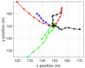
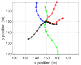
Figure 2: True trajectories in Scenario 1 (left) [12] and Scenario 2 (right). In Scenario 1, all targets are born at time step 1. In Scenario 2, the blue and the red targets are born at time step 1, whereas the green and the black targets are born at time step 21. The only target that dies during the simulations is the blue target, which dies at time step 40, when all targets are in close proximity. Targets positions every 10 time steps are marked with a circle, and their initial positions with a filled circle.

We consider the ground truth trajectories with $N_{s}=81$ time steps in Figure 2(left). We assess filter performance using Monte Carlo simulation with $N_{mc}=100$ runs. At each time step $k$, we measure the error between the true set $\mathbf{X}_{k}$ of trajectories and its estimate $\mathbf{\hat{X}}_{k}$, which differ depending on the problem formulation (see Section II). The error is determined by the linear programming metric $d\left(\cdot,\cdot\right)$ for sets of trajectories in [50] with parameters $p=2$, $c=10$ and $\gamma=1$. In our results, we only use the position elements to compute $d\left(\cdot,\cdot\right)$ and normalise the error by the considered time window such that the squared error at time $k$ becomes $d^{2}\left(\mathbf{X}_{k},\mathbf{\hat{X}}_{k}\right)/k$. The root mean square (RMS) error at a given time step is

$$d\left(k\right) =\sqrt{\frac{1}{N_{mc}k}\sum_{i=1}^{N_{mc}}d^{2}\left(\mathbf{X}_{k},\mathbf{\hat{X}}_{k}^{i}\right)},$$ (76)

where $\mathbf{\hat{X}}_{k}^{i}$ is the estimate of the set of trajectories at time $k$ in the $i$th Monte Carlo run.

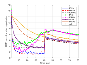
Figure 3: Trajectory metric error against time for the alive trajectories. Error increases at time step 40, when a target dies. On the whole, the TPMBM filter is the best performing filter followed by the TPMB filter.

We first proceed to analyse the error in estimating the set of alive trajectories. The RMS trajectory error against time is shown in Figure 3. For all filters, estimation error increases after time step 40, in which a target dies, and the rest of the targets are in close proximity. The TPMBM filter is the most accurate filter to estimate the alive trajectories. This is to be expected, as without approximations, the TPMBM filtering recursion provides the true posterior over the set of trajectories. The second best performing filter in general is the proposed TPMB filter. Its performance is slightly worse than TGNPMB after time step 40 but it is considerably better before time step 40. TPHD and TCPHD filters perform considerably worse, as they are less accurate approximations. The LMB filter performs worse than $\delta$-GLMB. $\delta$-GLMB is less accurate than PMBM, which is outperformed by TPMBM and TPMB.

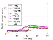
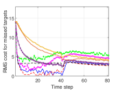
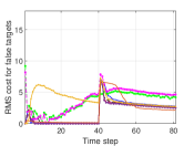
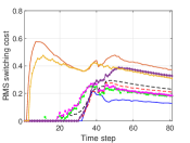
Figure 4: Decomposition of the trajectory metric error against time for the alive trajectories.

The squared trajectory metric $d^{2}\left(\cdot,\cdot\right)$ can be decomposed into the square costs for missed targets, false targets, localisation error of properly detected targets, and track switches [50]. The resulting RMS errors for the decomposed costs are shown in Figure 4. Before time step 40, all filters except LMB, TPHD and TCPHD have a negligible cost for false targets. Also, $\delta$-GLMB and PMBM show a higher error for missed targets, followed by TPHD, TCPHD and TGNPMBM. After time step 40, these filters increase their error mainly due to false and missed target errors, created by the disappearance of one trajectory. Track switching cost are small and quite similar for all filters based on sets of trajectories. $\delta$-GLMB and LMB are the only filters with track switches before targets get in close proximity, due to the IID birth, and provide the highest switching costs. PMBM filter has the third highest switching costs after time step 40. The errors obtained by the square sum of the generalised optimal sub-pattern assignment (GOSPA) metric ($\alpha=2$) [51] at each time step instead of $d^{2}\left(\cdot,\cdot\right)$ in (76) are quite similar to the trajectory metric errors, as, due to the choice of $\gamma$, the switching costs are small.

The average execution times in seconds of a single run (81 time steps) of our Matlab implementations with a 3.5 GHz Intel Xeon E5 processor are: 1.2 (TPMB), 7.0 (TPMBM), 0.7 (TGNPMB), 1.1 (TPHD), 1.1 (TCPHD), 5.8 (PMBM), 13.1 ($\delta$-GLMB) and 10.5 (LMB). The fastest algorithm is TGNPMB, though its performance is worse than TPMB. The TPMBM is slower than the other trajectory filters and PMBM but TPMBM is also the one with highest performance, as expected. There is a trade-off between computational complexity and accuracy in the selection of TPMBM, TPMB and TGNPMB. Trajectory filters are faster than $\delta$-GLMB/LMB even though the update past trajectory information in the $L$-scan window due to the considerably lower number of required global hypotheses to keep relevant information, see App. D.

We proceed to analyse the performance of the filters for different values of $L$ and different $p_{D}$ and $\overline{\lambda}^{C}$. In Table I, we show the resulting RMS error considering all time steps

$$d_{T}= \sqrt{\frac{1}{N_{s}}\sum_{k=1}^{N_{s}}d^{2}\left(k\right)}.$$ (77)

Increasing $L$ for the trajectory filters lowers the error, mainly due to improved localisation of past states. In general, the best performing filter is TPMBM, followed by TPMB. The TPMB approximation is accurate for the considered probabilities of detection and clutter intensity. As expected, if the clutter intensity increases, performance decreases for all filters. The higher the probability of detection, performance increases.

Table I: Trajectory metric errors (alive trajectories)

	TPMB			TPMBM			TGNPMB			TPHD			TCPHD			PMBM	GLMB	LMB
$L$	1	5	10	1	5	10	1	5	10	1	5	10	1	5	10	-	-	-
No change	5.18	4.84	4.82	4.87	4.50	4.49	5.30	4.98	4.97	7.87	7.69	7.69	7.50	7.30	7.30	5.73	7.62	8.64
$p_{D}=0.99$	4.91	4.73	4.73	4.55	4.36	4.35	4.66	4.47	4.46	7.17	7.06	7.06	7.07	6.96	6.96	5.46	7.38	7.48
$p_{D}=0.80$	5.52	5.02	5.00	5.38	4.89	4.88	5.94	5.54	5.52	8.74	8.52	8.52	8.04	7.80	7.79	6.27	7.52	9.48
$p_{D}=0.70$	5.92	5.21	5.18	5.91	5.24	5.22	7.02	6.55	6.53	9.12	8.88	8.87	8.47	8.20	8.20	6.76	8.43	10.38
$\overline{\lambda}^{C}=20$	5.27	4.92	4.91	4.98	4.63	4.62	6.39	6.18	6.17	8.04	7.87	7.86	7.55	7.36	7.36	5.90	8.19	9.12
$\overline{\lambda}^{C}=30$	5.27	4.96	4.94	4.95	4.62	4.61	7.50	7.39	7.39	8.11	7.95	7.95	7.62	7.44	7.44	5.96	8.51	9.44
$\overline{\lambda}^{C}=40$	5.32	5.01	4.99	5.05	4.73	4.72	8.14	8.04	8.04	8.16	8.01	8.00	7.73	7.56	7.56	6.12	8.86	9.79

Finally, we consider the estimation of the set of all trajectories. TPHD and TCPHD filters are not included as they are not suitable for this problem [28]. The RMS errors (77) are shown in Table II. As before, error decreases by increasing $L$, and TPMBM is generally the best algorithm followed by TPMB. PMBM performs worse than these filters, but better than $\delta$-GLMB and LMB.

The average execution times in seconds of a single run (81 time steps) for $p_{D}=0.9$, $\overline{\lambda}^{C}=10$, $L=5$, and the estimation of all trajectories are: 1.5 (TPMB), 7.9 (TPMBM), 0.9 (TGNPMB), 5.8 (PMBM), 13.1 ($\delta$-GLMB) and 10.5 (LMB). Compared to tracking alive trajectories, there is an increase in the execution time in the trajectory filters. The sequential track estimators, PMBM, $\delta$-GLMB and LMB have the same computational burden to solve both problems, as they only differ in the estimated set of trajectories.

Table II: Trajectory metric errors (all trajectories)

	TPMB			TPMBM			TGNPMB			PMBM	GLMB	LMB
$L$	1	5	10	1	5	10	1	5	10	-	-	-
No change	3.11	2.37	2.34	3.09	2.36	2.34	4.31	3.88	3.86	4.58	7.05	8.79
$p_{D}=0.99$	2.52	2.07	2.04	2.50	2.06	2.04	3.11	2.78	2.77	4.17	6.68	6.74
$p_{D}=0.80$	3.71	2.77	2.73	3.66	2.75	2.72	5.22	4.70	4.68	5.15	7.52	9.63
$p_{D}=0.70$	4.43	3.26	3.20	4.41	3.29	3.25	6.56	6.00	5.98	5.70	8.02	10.84
$\overline{\lambda}^{C}=20$	3.23	2.52	2.49	3.18	2.49	2.47	6.22	5.99	5.99	4.81	7.75	9.07
$\overline{\lambda}^{C}=30$	3.29	2.64	2.61	3.24	2.63	2.60	7.63	7.53	7.52	5.02	8.20	9.52
$\overline{\lambda}^{C}=40$	3.31	2.69	2.66	3.29	2.70	2.68	8.39	8.30	8.30	5.17	8.69	9.97

VI-B Range-bearings measurements

This section analyses a scenario with range-bearings measurements [52], and the same dynamic model as in Section VI-A. We have $l\left(z|x\right)=\mathcal{N}\left(z;h\left(x\right),R\right)$ with

$$h\left(x\right) =\left[\sqrt{\left(p_{x}-s_{x}\right)^{2}+\left(p_{y}-s_{y}\right)^{2}},\arctan\left(\frac{p_{y}-s_{y}}{p_{x}-s_{x}}\right)\right]^{T}$$

where $\left[s_{x},s_{y}\right]=\left[100,100\right]$ is the sensor location, and $R=\text{diag}([1,\left(2\pi/180\right)^{2}])$.

We consider multi-Bernoulli birth with four Bernoullis with Gaussian densities located at point sources [13]. The probabilities of existence are 0.01, the covariance matrices are $\text{diag}([9,1,9,1])$, and the means are located at $[140,0,170,0]^{T}$, $[165,0,155,0]^{T}$, $[150,0,160,0]^{T}$ and $[160,0,150,0]^{T}$, respectively. The filters with Poisson RFS birth model have an intensity that matches the PHD, which is a Gaussian mixture. We consider $p_{D}=0.9$ and $\lambda^{C}\left(z\right)=\overline{\lambda}^{C}u_{A}\left(z\right)$ where $A=\left[10,200\right]\times\left[0,\pi/2\right]$ and $\overline{\lambda}^{C}=10$.

We have implemented the filtering recursions using an extended Kalman filter (EKF) [53]. The EKF linearises $h\left(\cdot\right)$ at the current mean of each trajectory density using a first-order Taylor series. Then, the multi-target filtering recursions proceed as in the affine measurement case, which is a direct extension of the linear case.

The ground truth set of trajectories, with $81$ time steps, is shown in Figure 2 (right). The trajectory filters are implemented with $L=5$. The RMS trajectory error for alive trajectories is shown in Figure 5. In this case, the TPMB and TMB filters are the best performing filters followed by the TPMBM filter and TGNPMB. Sequential track estimators, PMBM and $\delta$-GLMB perform quite similarly, and LMB works slightly better than these for the considered parameters. TPHD and TCPHD have lower performance.

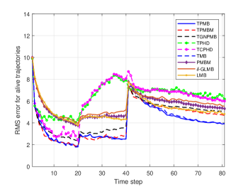
Figure 5: Trajectory metric error against time for the alive trajectories in the range-bearings scenario. The TPMB and TMB filters are the best performing filters, with TPMB being faster than TMB.

The average execution times in seconds (81 time steps) are: 1.8 (TPMB), 5.9 (TPMBM), 0.6 (TGNPMB), 0.9 (TPHD), 0.9 (TCPHD), 5.5 (TMB), 4.9 (PMBM), 14.8 ($\delta$-GLMB) and 30.1 (LMB). The filters with Poisson birth are faster than with multi-Bernoulli birth. The joint prediction and update $\delta$-GLMB is faster than LMB [22] in this scenario.

VII Conclusions

We have proposed two Poisson multi-Bernoulli filters for sets of trajectories to perform multiple target tracking. One TPMB filter contains information on the set of alive trajectories and the other on the set of all trajectories, which include alive and dead trajectories. We have also proposed Gaussian implementations of the filters.

The resulting filters offer a trade-off between computational complexity and accuracy. They are faster than TPMBM filters but typically have worse performance. The TPMB filters are considerably more accurate than TPHD and TCPHD filters, but with higher computational complexity. Computational and performance benefits with respect to $\delta$-GLMB and LMB filters are shown in two simulated scenarios.

Trajectory Poisson multi-Bernoulli filters: Supplementary material

Appendix A

In this appendix, we prove that if we integrate the auxiliary variables in $\widetilde{f}_{k^{\prime}|k}\left(\cdot\right)$, see (9), we recover $f_{k^{\prime}|k}\left(\cdot\right)$. That is, we prove that

$$\sum_{u_{1:n}\in\mathbb{\mathbb{U}}_{k}^{n}}\widetilde{f}_{k^{\prime}|k}\left(\left\{\left(u_{1},X_{1}\right),...,\left(u_{n},X_{n}\right)\right\}\right)$$

$$\quad=f_{k^{\prime}|k}\left(\left\{X_{1},...,X_{n}\right\}\right).$$ (78)

We first obtain two preliminary results with only a Poisson component and a multi-Bernoulli mixture. Then, we proceed to prove the PMBM case.

A-A PPP

Integrating out the auxiliary variables in $\widetilde{f}_{k^{\prime}|k}^{p}\left(\cdot\right)$, we obtain

$$\sum_{u_{1:n}\in\mathbb{\mathbb{U}}_{k^{\prime}|k}^{n}}\widetilde{f}_{k^{\prime}|k}^{p}\left(\left\{\left(u_{1},X_{1}\right)...,\left(u_{n},X_{n}\right)\right\}\right)$$

$$=e^{-\int\lambda_{k^{\prime}|k}\left(X\right)dX}\left[\prod_{i=1}^{n}\lambda_{k^{\prime}|k}\left(X_{i}\right)\right]\left[\sum_{u_{1:n}\in\mathbb{\mathbb{U}}_{k^{\prime}|k}^{n}}\prod_{i=1}^{n}\delta_{0}\left[u_{i}\right]\right]$$

$$=f_{k^{\prime}|k}^{p}\left(\left\{X_{1},...,X_{n}\right\}\right).$$ (79)

A-B Multi-Bernoulli mixture

We first note that if $\lambda_{k^{\prime}|k}\left(\cdot\right)=0$, then, the PMBM (8) is an MBM. Using [9, Eq. (4.127)], for existence probabilities smaller than one, the MBM with auxiliary variables can be written as

$$\widetilde{f}_{k^{\prime}|k}^{mbm}\left(\left\{\left(u_{1},X_{1}\right)...,\left(u_{n},X_{n}\right)\right\}\right)$$

$$=\sum_{a\in\mathcal{A}_{k^{\prime}|k}}w_{k^{\prime}|k}^{a}\left[\prod_{i=1}^{n_{k^{\prime}|k}}\left(1-r_{k^{\prime}|k}^{i,a^{i}}\right)\right]$$

$$\sum_{1\leq i_{1}\neq...,\neq i_{n}\leq n_{k^{\prime}|k}}\prod_{p=1}^{n}\frac{r_{k^{\prime}|k}^{i_{p},a_{p}^{i}}}{1-r_{k^{\prime}|k}^{i_{p},a_{p}^{i}}}p_{k^{\prime}|k}^{i_{p},a^{i_{p}}}\left(X_{p}\right)\delta_{i_{p}}\left[u_{p}\right]$$ (80)

If we integrate out the auxiliary variables in (80), we obtain the MBM without auxiliary variables

$$\sum_{u_{1:n}\in\mathbb{\mathbb{U}}_{k^{\prime}|k}^{n}}\widetilde{f}_{k^{\prime}|k}^{mbm}\left(\left\{\left(u_{1},X_{1}\right)...,\left(u_{n},X_{n}\right)\right\}\right)$$

$$=\sum_{a\in\mathcal{A}_{k^{\prime}|k}}w_{k^{\prime}|k}^{a}\left[\prod_{i=1}^{n_{k^{\prime}|k}}\left(1-r_{k^{\prime}|k}^{i,a^{i}}\right)\right]\sum_{1\leq i_{1}\neq...,\neq i_{n}\leq n_{k^{\prime}|k}}$$

$$\,\left[\prod_{p=1}^{n}\frac{r_{k^{\prime}|k}^{i_{p},a_{p}^{i}}}{1-r_{k^{\prime}|k}^{i_{p},a_{p}^{i}}}p_{k^{\prime}|k}^{i_{p},a^{i_{p}}}\left(X_{p}\right)\right]\left[\sum_{u_{1:n}\in\mathbb{\mathbb{U}}_{k^{\prime}|k}^{n}}\prod_{p=1}^{n}\delta_{i_{p}}\left[u_{p}\right]\right]$$ (81)

$$=f_{k^{\prime}|k}^{mbm}\left(\left\{X_{1}...,X_{n}\right\}\right).$$ (82)

If some existence probabilities are equal to one, the derivation is analogous, but removing the corresponding $\left(1-r_{k^{\prime}|k}^{i,a^{i}}\right)$ in the numerator and denominator in (80).

A-C PMBM

We can write the PMBM (8) as

$$f_{k^{\prime}|k}\left(\left\{X_{1},...,X_{n}\right\}\right) =\sum_{\mathbf{Y}\subseteq\left\{X_{1},...,X_{n}\right\}}f_{k^{\prime}|k}^{p}\left(\mathbf{Y}\right)f_{k^{\prime}|k}^{mbm}\left(\mathbf{X}_{k^{\prime}}\setminus\mathbf{Y}\right)$$ (83)

$$=\sum_{j=0}^{n}\sum_{\sigma\in\Gamma_{n,j}}f_{k^{\prime}|k}^{p}\left(\left\{X_{\sigma_{1}},...,X_{\sigma_{j}}\right\}\right)$$

$$\quad\times f_{k^{\prime}|k}^{mbm}\left(\left\{X_{\sigma_{j+1}},...,X_{\sigma_{n}}\right\}\right)$$ (84)

where $\Gamma_{n,j}$ is the set that contains all possible sets $\sigma=\left\{\sigma_{1},...,\sigma_{j}\right\}$ of $j$ elements from $\left\{1,...,n\right\}$ and $\left\{\sigma_{j+1},...,\sigma_{n}\right\}=\left\{1,...,n\right\}\setminus\left\{\sigma_{1},...,\sigma_{j}\right\}$. The cardinality of set $\Gamma_{n,j}$ is

$$\left|\Gamma_{n,j}\right|=\left(\begin{array}[]{c}n\\ j\end{array}\right).$$ (85)

Using these formulas on the PMBM density with auxiliary variables, we have

$$\widetilde{f}_{k^{\prime}|k}\left(\left\{\left(u_{1},X_{1}\right)...,\left(u_{n},X_{n}\right)\right\}\right)$$

$$=\sum_{j=0}^{n}\sum_{\sigma\in\Gamma_{n,j}}\widetilde{f}_{k^{\prime}|k}^{p}\left(\left\{\left(u_{\sigma_{1}},X_{\sigma_{1}}\right),...,\left(u_{\sigma_{j}},X_{\sigma_{j}}\right)\right\}\right)$$

$$\times\widetilde{f}_{k^{\prime}|k}^{mbm}\left(\left\{\left(u_{\sigma_{j+1}},X_{\sigma_{j+1}}\right),...,\left(u_{\sigma_{n}},X_{\sigma_{n}}\right)\right\}\right)$$ (86)

Then, integrating out the auxiliary variables

$$\sum_{u_{1:n}\in\mathbb{\mathbb{U}}_{k^{\prime}|k}^{n}}\widetilde{f}_{k^{\prime}|k}\left(\left\{\left(u_{1},X_{1}\right)...,\left(u_{n},X_{n}\right)\right\}\right)$$

$$=\sum_{u_{1:n}\in\mathbb{\mathbb{U}}_{k^{\prime}|k}^{n}}\sum_{j=0}^{n}\sum_{\sigma\in\Gamma_{n,j}}\widetilde{f}_{k^{\prime}|k}^{p}\left(\left\{\left(u_{\sigma_{1}},X_{\sigma_{1}}\right),...,\left(u_{\sigma_{j}},X_{\sigma_{j}}\right)\right\}\right)$$

$$\times\widetilde{f}_{k^{\prime}|k}^{mbm}\left(\left\{\left(u_{\sigma_{j+1}},X_{\sigma_{j+1}}\right),...,\left(u_{\sigma_{n}},X_{\sigma_{n}}\right)\right\}\right)$$ (87)

$$=\sum_{j=0}^{n}\sum_{\sigma\in\Gamma_{n,j}}\left[\sum_{u_{\sigma_{1:j}}\in\mathbb{\mathbb{N}}_{0}^{j}}\widetilde{f}_{k^{\prime}|k}^{p}\left(\left\{\left(u_{\sigma_{1}},X_{\sigma_{1}}\right),...,\left(u_{\sigma_{j}},X_{\sigma_{j}}\right)\right\}\right)\right]$$

$$\times\left[\sum_{u_{\sigma_{j+1:n}}\in\mathbb{\mathbb{N}}_{0}^{n-j}}\widetilde{f}_{k^{\prime}|k}^{mbm}\left(\left\{\left(u_{\sigma_{j+1}},X_{\sigma_{j+1}}\right),...,\left(u_{\sigma_{n}},X_{\sigma_{n}}\right)\right\}\right)\right]$$ (88)

Applying the results in the previous two subsections, we finish the proof of (78).

Appendix B

In Section B-A, we prove Proposition 2. We also prove in Section B-B that the resulting density from the KLD minimisation also matches the PHD. Finally, we prove Lemma 3 in Section B-C.

B-A KLD minimisation

The augmented single trajectory space $\mathbb{\mathbb{U}}_{k^{\prime}|k}\times T_{\left(k^{\prime}\right)}$ can be written as the union of disjoint spaces $\mathbb{\mathbb{U}}_{k^{\prime}|k}\times T_{\left(k^{\prime}\right)}=\uplus_{u=0}^{n_{k^{\prime}|k}}\left\{u\right\}\times T_{\left(k^{\prime}\right)}$. Therefore, given a finite set $\widetilde{\mathbf{X}}_{k^{\prime}}\subset\mathbb{\mathbb{U}}_{k^{\prime}|k}\times T_{\left(k^{\prime}\right)}$, we can write $\widetilde{\mathbf{X}}_{k^{\prime}}=\widetilde{\mathbf{Y}}_{k^{\prime}}\uplus\widetilde{\mathbf{X}}_{k^{\prime}}^{1}\uplus...\uplus\widetilde{\mathbf{X}}_{k^{\prime}}^{n_{k^{\prime}|k}}$, where $\widetilde{\mathbf{Y}}_{k^{\prime}}\subset\left\{0\right\}\times T_{\left(k^{\prime}\right)}$ and $\widetilde{\mathbf{X}}_{k^{\prime}}^{i}\subset\left\{i\right\}\times T_{\left(k^{\prime}\right)}$, to obtain [9, Eq. (3.53)]

$$\mathrm{D}\left(\widetilde{f}\left\|\widetilde{q}\right.\right)$$

$$\,=\int\widetilde{f}\left(\widetilde{\mathbf{X}}_{k^{{}^{\prime}}}\right)\log\frac{\widetilde{f}\left(\widetilde{\mathbf{X}}_{k^{{}^{\prime}}}\right)}{\widetilde{q}\left(\widetilde{\mathbf{X}}_{k^{{}^{\prime}}}\right)}\delta\widetilde{\mathbf{X}}_{k^{{}^{\prime}}}$$

$$\,=\int\int...\int\widetilde{f}\left(\widetilde{\mathbf{Y}}_{k^{\prime}}\uplus\widetilde{\mathbf{X}}_{k^{\prime}}^{1}\uplus...\uplus\widetilde{\mathbf{X}}_{k^{\prime}}^{n_{k^{\prime}|k}}\right)$$

$$\,\times\log\frac{\widetilde{f}\left(\widetilde{\mathbf{Y}}_{k^{\prime}}\uplus\widetilde{\mathbf{X}}_{k^{\prime}}^{1}\uplus...\uplus\widetilde{\mathbf{X}}_{k^{\prime}}^{n_{k^{\prime}|k}}\right)}{\widetilde{q}\left(\widetilde{\mathbf{Y}}_{k^{\prime}}\uplus\widetilde{\mathbf{X}}_{k^{\prime}}^{1}\uplus...\uplus\widetilde{\mathbf{X}}_{k^{\prime}}^{n_{k^{\prime}|k}}\right)}\delta\widetilde{\mathbf{Y}}_{k^{\prime}}\delta\widetilde{\mathbf{X}}_{k^{\prime}}^{1}...\delta\widetilde{\mathbf{X}}_{k^{\prime}}^{n_{k^{\prime}|k}}$$

$$=c-\int\widetilde{f}_{k^{\prime}|k}^{p}\left(\widetilde{\mathbf{Y}}_{k^{\prime}}\right)\log\widetilde{q}^{p}\left(\widetilde{\mathbf{Y}}_{k^{\prime}}\right)\delta\widetilde{\mathbf{Y}}_{k^{\prime}}$$

$$\quad-\sum_{i=1}^{n_{k^{\prime}|k}}\int\sum_{a\in\mathcal{A}_{k^{\prime}|k}}w_{k^{\prime}|k}^{a}\widetilde{f}_{k^{\prime}|k}^{i,a^{i}}\left(\widetilde{\mathbf{X}}_{k^{\prime}}^{i}\right)\log\widetilde{q}^{i,1}\left(\widetilde{\mathbf{X}}_{k^{\prime}}^{i}\right)\delta\widetilde{\mathbf{X}}_{k^{\prime}}^{i}$$ (89)

where $c$ is a constant that does not depend on $\widetilde{q}\left(\cdot\right)$. Maximising with respect to $\widetilde{q}^{p}\left(\cdot\right)$, $\widetilde{q}^{1,1}\left(\cdot\right)$, …,$\widetilde{q}^{n_{k^{\prime}|k},1}\left(\cdot\right)$, we get

$$\widetilde{q}^{p}\left(\widetilde{\mathbf{Y}}_{k^{\prime}}\right) =\widetilde{f}_{k^{\prime}|k}^{p}\left(\widetilde{\mathbf{Y}}_{k^{\prime}}\right)$$ (90)

$$\widetilde{q}^{i,1}\left(\widetilde{\mathbf{X}}_{k^{\prime}}^{i}\right) =\sum_{a\in\mathcal{A}_{k^{\prime}|k}}w_{k^{\prime}|k}^{a}\widetilde{f}_{k^{\prime}|k}^{i,a^{i}}\left(\widetilde{\mathbf{X}}_{k^{\prime}}^{i}\right).$$ (91)

Using (12) and identifying terms w.r.t. (15), we have that the existence probability $r^{i}$ and single-trajectory density $p^{i}\left(\cdot\right)$ of $\widetilde{q}^{i,1}\left(\cdot\right)$ are

$$r^{i} =\sum_{a\in\mathcal{A}_{k^{\prime}|k}}w_{k^{\prime}|k}^{a}r_{k^{\prime}|k}^{i,a^{i}}$$ (92)

$$p^{i}\left(X\right) =\frac{\sum_{a\in\mathcal{A}_{k^{\prime}|k}}w_{k^{\prime}|k}^{a}r_{k^{\prime}|k}^{i,a^{i}}p_{k^{\prime}|k}^{i,a^{i}}\left(X\right)}{\sum_{a\in\mathcal{A}_{k^{\prime}|k}}w_{k^{\prime}|k}^{a}r_{k^{\prime}|k}^{i,a^{i}}}.$$ (93)

By grouping similar local hypotheses, $r^{i}$ and $p^{i}\left(\cdot\right)$ become those given in Proposition 2, which finishes the proof.

B-B Matching the PHD

In this section, we show that, for KLD minisimation in the previous section, it holds that the PHD of $\widetilde{f}\left(\cdot\right)$ is the same as the PHD of $\widetilde{q}\left(\cdot\right)$. In Sections B-B1 and B-B2, we calculate the PHD of $\widetilde{f}\left(\cdot\right)$ and $\widetilde{q}\left(\cdot\right)$, respectively.

B-B1 PHD of $\widetilde{f}\left(\cdot\right)$

The PHD $D_{\widetilde{f}}\left(\cdot\right)$ of density $\widetilde{f}\left(\cdot\right)$ for sets of trajectories, which is given by (9), is [9, 28]

$$D_{\widetilde{f}}\left(\widetilde{X}\right) =\int\widetilde{f}\left(\left\{\widetilde{X}\right\}\cup\widetilde{\mathbf{X}}_{k^{\prime}}\right)\delta\widetilde{\mathbf{X}}_{k^{\prime}}$$

$$=\int\widetilde{f}\left(\left\{\widetilde{X}\right\}\cup\widetilde{\mathbf{Y}}_{k^{\prime}}\uplus\widetilde{\mathbf{X}}_{k^{\prime}}^{1}\uplus...\uplus\widetilde{\mathbf{X}}_{k^{\prime}}^{n_{k^{\prime}|k}}\right)$$

$$\quad\delta\widetilde{\mathbf{Y}}_{k^{\prime}}\delta\widetilde{\mathbf{X}}_{k^{\prime}}^{1}...\delta\widetilde{\mathbf{X}}_{k^{\prime}}^{n_{k^{\prime}|k}}$$ (94)

where we have applied the decomposition of the set integral into disjoint spaces, see Section B-A.

If $\widetilde{X}=\left(0,X\right)\in\left\{0\right\}\times T_{\left(k^{\prime}\right)}$, then the PHD is

$$D_{\widetilde{f}}\left(\widetilde{X}\right) =\int\widetilde{f}_{k^{\prime}|k}^{p}\left(\left\{\widetilde{X}\right\}\cup\widetilde{\mathbf{Y}}_{k^{\prime}}\right)\sum_{a\in\mathcal{A}_{k^{\prime}|k}}w_{k^{\prime}|k}^{a}$$

$$\,\times\prod_{i=1}^{n_{k^{\prime}|k}}\left[\widetilde{f}_{k^{\prime}|k}^{i,a^{i}}\left(\widetilde{\mathbf{X}}_{k^{\prime}}^{i}\right)\right]\delta\widetilde{\mathbf{Y}}_{k^{\prime}}\delta\widetilde{\mathbf{X}}_{k^{\prime}}^{1}...\delta\widetilde{\mathbf{X}}_{k^{\prime}}^{n_{k^{\prime}|k}}$$

$$=\int\widetilde{f}_{k^{\prime}|k}^{p}\left(\left\{\widetilde{X}\right\}\cup\widetilde{\mathbf{Y}}_{k^{\prime}}\right)\delta\widetilde{\mathbf{Y}}_{k^{\prime}}$$

$$=\lambda_{k^{\prime}|k}\left(X\right)$$ (95)

where the last line follows directly as it corresponds to the PHD of the PPP $\widetilde{f}_{k^{\prime}|k}^{p}\left(\cdot\right)$.

If $\widetilde{X}=\left(u,X\right)\in\left\{u\right\}\times T_{\left(k^{\prime}\right)}$, $u\in\left\{1,...,n_{k^{\prime}|k}\right\}$, then the PHD is

$$D_{\widetilde{f}}\left(\widetilde{X}\right) =\int\widetilde{f}_{k^{\prime}|k}^{p}\left(\widetilde{\mathbf{Y}}_{k^{\prime}}\right)\sum_{a\in\mathcal{A}_{k^{\prime}|k}}w_{k^{\prime}|k}^{a}\widetilde{f}_{k^{\prime}|k}^{u,a^{u}}\left(\left\{\widetilde{X}\right\}\cup\widetilde{\mathbf{X}}_{k^{\prime}}^{u}\right)$$

$$\,\times\prod_{i=1,i\neq u}^{n_{k^{\prime}|k}}\left[\widetilde{f}_{k^{\prime}|k}^{i,a^{i}}\left(\widetilde{\mathbf{X}}_{k^{\prime}}^{i}\right)\right]\delta\widetilde{\mathbf{Y}}_{k^{\prime}}\delta\widetilde{\mathbf{X}}_{k^{\prime}}^{1}...\delta\widetilde{\mathbf{X}}_{k^{\prime}}^{n_{k^{\prime}|k}}$$

$$=\sum_{a\in\mathcal{A}_{k^{\prime}|k}}w_{k^{\prime}|k}^{a}\int\widetilde{f}_{k^{\prime}|k}^{u,a^{u}}\left(\left\{\widetilde{X}\right\}\cup\widetilde{\mathbf{X}}_{k^{\prime}}^{u}\right)\delta\widetilde{\mathbf{X}}_{k^{\prime}}^{u}$$

$$=\sum_{a\in\mathcal{A}_{k^{\prime}|k}}w_{k^{\prime}|k}^{a}r_{k^{\prime}|k}^{u,a^{u}}p_{k^{\prime}|k}^{u,a^{u}}\left(X\right)$$ (96)

B-B2 PHD of $\widetilde{q}\left(\cdot\right)$

We calculate the PHD of $\widetilde{q}\left(\cdot\right)$, which is given by (15) and Proposition 2, using (94). If $\widetilde{X}=\left(0,X\right)\in\left\{0\right\}\times T_{\left(k^{\prime}\right)}$, then the PHD is

$$D_{\widetilde{q}}\left(\widetilde{X}\right) =\int\int...\int\widetilde{q}^{p}\left(\left\{\widetilde{X}\right\}\cup\widetilde{\mathbf{Y}}_{k^{\prime}}\right)$$

$$\>\times\prod_{i=1}^{n_{k^{\prime}|k}}\left[\widetilde{q}^{i,1}\left(\widetilde{\mathbf{X}}_{k^{\prime}}^{i}\right)\right]\delta\widetilde{\mathbf{Y}}_{k^{\prime}}\delta\widetilde{\mathbf{X}}_{k^{\prime}}^{1}...\delta\widetilde{\mathbf{X}}_{k^{\prime}}^{n_{k^{\prime}|k}}$$

$$=\int\widetilde{q}^{p}\left(\left\{\widetilde{X}\right\}\cup\widetilde{\mathbf{Y}}_{k^{\prime}}\right)\delta\widetilde{\mathbf{Y}}_{k^{\prime}}$$

$$=\lambda_{k^{\prime}|k}\left(X\right).$$ (97)

If $\widetilde{X}=\left(u,X\right)\in\left\{u\right\}\times T_{\left(k^{\prime}\right)}$, $u\in\left\{1,...,n_{k^{\prime}|k}\right\}$, then the PHD is

$$D_{\widetilde{q}}\left(\widetilde{X}\right) =\int\int...\int\widetilde{q}^{p}\left(\widetilde{\mathbf{Y}}_{k^{\prime}}\right)\widetilde{q}^{u,1}\left(\left\{\widetilde{X}\right\}\cup\widetilde{\mathbf{X}}_{k^{\prime}}^{u}\right)$$

$$\,\times\prod_{i=1,,i\neq u}^{n_{k^{\prime}|k}}\left[\widetilde{q}^{i,1}\left(\widetilde{\mathbf{X}}_{k^{\prime}}^{i}\right)\right]\delta\widetilde{\mathbf{Y}}_{k^{\prime}}\delta\widetilde{\mathbf{X}}_{k^{\prime}}^{1}...\delta\widetilde{\mathbf{X}}_{k^{\prime}}^{n_{k^{\prime}|k}}$$

$$=\int\widetilde{q}^{u,1}\left(\left\{\widetilde{X}\right\}\cup\widetilde{\mathbf{X}}_{k^{\prime}}^{u}\right)\delta\widetilde{\mathbf{X}}_{k^{\prime}}^{u}$$

$$=\sum_{a\in\mathcal{A}_{k^{\prime}|k}}w_{k^{\prime}|k}^{a}r_{k^{\prime}|k}^{u,a^{i}}p_{k^{\prime}|k}^{u,a^{i}}\left(X\right).$$ (98)

We can see that the PHD of $\widetilde{q}\left(\cdot\right)$, which is given by (97) and (98), coincides with the PHD of $\widetilde{f}\left(\cdot\right)$, which is given by (95) and (96).

B-C KLD bound

In this section, we prove Lemma 3. We have

$$\mathrm{D}\left(f_{k^{\prime}|k}\left\|q\right.\right) =\sum_{n=0}^{\infty}\frac{1}{n!}\int f_{k^{\prime}|k}\left(\left\{X_{1},...,X_{n}\right\}\right)$$

$$\,\times\log\frac{f_{k^{\prime}|k}\left(\left\{X_{1},...,X_{n}\right\}\right)}{q\left(\left\{X_{1},...,X_{n}\right\}\right)}dX_{1:n}$$

$$=\sum_{n=0}^{\infty}\frac{1}{n!}\int\sum_{u_{1:n}}\widetilde{f}{}_{k^{\prime}|k}\left(\left\{\left(u_{1},X_{1}\right),...,\left(u_{n}X_{n}\right)\right\}\right)$$

$$\,\times\log\frac{\sum_{u_{1:n}}\widetilde{f}{}_{k^{\prime}|k}\left(\left\{\left(u_{1},X_{1}\right),...,\left(u_{n}X_{n}\right)\right\}\right)}{\sum_{u_{1:n}}\widetilde{q}\left(\left\{\left(u_{1},X_{1}\right),...,\left(u_{n}X_{n}\right)\right\}\right)}dX_{1:n}$$ (99)

where we have used (78). Applying the log sum inequality [54] inside the integral, we obtain

$$\mathrm{D}\left(f_{k^{\prime}|k}\left\|q\right.\right) \leq\sum_{n=0}^{\infty}\frac{1}{n!}\int\sum_{u_{1:n}}\widetilde{f}{}_{k^{\prime}|k}\left(\left\{\left(u_{1},X_{1}\right),...,\left(u_{n}X_{n}\right)\right\}\right)$$

$$\,\times\log\frac{\widetilde{f}{}_{k^{\prime}|k}\left(\left\{\left(u_{1},X_{1}\right),...,\left(u_{n}X_{n}\right)\right\}\right)}{\widetilde{q}\left(\left\{\left(u_{1},X_{1}\right),...,\left(u_{n}X_{n}\right)\right\}\right)}dX_{1:n}$$

$$=\mathrm{D}\left(\widetilde{f}{}_{k^{\prime}|k}\left\|\widetilde{q}\right.\right).$$ (100)

This completes the proof of Lemma 3.

Appendix C

This appendix provides the expression of the mean and covariance matrix of the density $p_{k|k}^{i}\left(\cdot\right)$ of updated Bernoulli component $i$ after the GMTPMB updates. The case for the estimation of the set of alive trajectories is given in Section C-A, and the case of all trajectories in Section C-B.

C-A Set of alive trajectories

The updated Bernoulli component $i$ of the resulting PMB density from Lemma 7 have $r_{k|k}^{i}$ given by (17), and mean and covariance matrix

$$\overline{x}_{k|k}^{i} =\sum_{a^{i}=1:r_{k|k}^{i,a^{i}}>0}^{h^{i}}\left[\frac{\overline{w}_{k|k}^{i,a^{i}}r_{k|k}^{i,a^{i}}}{r_{k|k}^{i}}\overline{u}_{k|k}^{i,a^{i}}\right]$$ (101)

$$P_{k|k}^{i} =\sum_{a^{i}=1:r_{k|k}^{i,a^{i}}>0}^{h^{i}}\left[\frac{\overline{w}_{k|k}^{i,a^{i}}r_{k|k}^{i,a^{i}}}{r_{k|k}^{i}}\left(W_{k|k}^{i,a^{i}}+\overline{u}_{k|k}^{i,a^{i}}\left(\overline{u}_{k|k}^{i,a^{i}}\right)^{T}\right)\right]$$

$$\quad-\overline{x}_{k|k}^{i}\left(\overline{x}_{k|k}^{i}\right)^{T}$$ (102)

where $\overline{w}_{k^{\prime}|k}^{i,a^{i}}$ is given by (19), which requires (7) to relate to local hypotheses weights. Local hypotheses with $r_{k|k}^{i,a^{i}}=0$ have no associated $\overline{u}_{k|k}^{i,a^{i}}$ and $W_{k|k}^{i,a^{i}}$ so they are not considered in the above sums.

C-B Set of all trajectories

The updated Bernoulli component $i$ of the resulting PMB density from Lemma 9 is of the form (66). For alive trajectories, $l=k$, we perform moment matching to obtain $\overline{x}_{k|k}^{i}\left(k\right)$ and $P_{k|k}^{i}\left(k\right)$ in (66), which yields

$$\overline{x}_{k|k}^{i}\left(k\right) =\sum_{a^{i}=1:r_{k|k}^{i,a^{i}}>0}^{h^{i}}\left[\frac{\overline{w}_{k|k}^{i,a^{i}}r_{k|k}^{i,a^{i}}\beta_{k|k}^{i,a^{i}}\left(k\right)}{\check{r}_{k|k}^{i}}\overline{u}_{k|k}^{i,a^{i}}\left(k\right)\right]$$ (103)

$$P_{k|k}^{i}\left(k\right) =\sum_{a^{i}=1:r_{k|k}^{i,a^{i}}>0}^{h^{i}}\left[\frac{\overline{w}_{k|k}^{i,a^{i}}r_{k|k}^{i,a^{i}}\beta_{k|k}^{i,a^{i}}\left(k\right)}{\check{r}_{k|k}^{i}}\left(W_{k|k}^{i,a^{i}}\left(k\right)\right.\right.$$

$$\left.\left.+\overline{u}_{k|k}^{i,a^{i}}\left(k\right)\left(\overline{u}_{k|k}^{i,a^{i}}\left(k\right)\right)^{T}\right)\right]-\overline{x}_{k|k}^{i}\left(k\right)\left(\overline{x}_{k|k}^{i}\left(k\right)\right)^{T}$$ (104)

$$\check{r}_{k|k}^{i} =\sum_{a^{i}=1:r_{k|k}^{i,a^{i}}>0}^{h^{i}}\overline{w}_{k|k}^{i,a^{i}}r_{k|k}^{i,a^{i}}\beta_{k|k}^{i,a^{i}}\left(k\right).$$ (105)

Appendix D

We proceed to determine the number of global hypotheses after the first update for the filters based on Poisson birth model and multi-Bernoulli birth model (labelled or not). We focus on the first update as the number of global hypotheses is closed-form for all filters and we can draw important insights into how the different filters deal with hypotheses. We first consider updating a multi-Bernoulli RFS birth with $n$ Bernoullis (with probability of existence $r\in\left(0,1\right)$) with the MBM and MBM₀₁ ($\delta$-GLMB) filters. This result is equivalent for filters based on targets and trajectories. Also, the number of global hypotheses is not affected by labelling the MBM and the MBM₀₁ [12, Sec. IV][13, Sec. III.C].

Suppose we receive $m$ measurements. Then, for the MBM update (which corresponds to the PMBM update with Poisson intensity equal to zero), we obtain that the number of updated global hypotheses is

$$N_{A}^{\mathrm{MBM}}\left(m,n\right)=\sum_{p=0}^{\min\left(m,n\right)}p!\left(\begin{array}[]{c}m\\ p\end{array}\right)\left(\begin{array}[]{c}n\\ p\end{array}\right)$$ (106)

where $p$ represents the number of detected targets. The explanation of (106) is as follows. The number of ways of selecting $p$ measurements from $m$ measurements is $\left(\begin{array}[]{c}m\\ p\end{array}\right)$. The number of ways of selecting $p$ targets from $n$ Bernoullis is $\left(\begin{array}[]{c}n\\ p\end{array}\right)$. Finally, the number of ways of associating the detected measurements with the detected targets is $p!$ and we must sum over all possible $p$, which goes from 0 to $\min\left(m,n\right)$ to yield (106).

When we consider an MBM₀₁ ($\delta$-GLMB) update, the multi-Bernoulli is converted into an MBM₀₁ ($\delta$-GLMB), in which targets have deterministic existence rather than probabilistic. This step results in an MBM₀₁ ($\delta$-GLMB) with $2^{n}$ components/global hypotheses [12, Sec. IV][22, Sec. IV.C.1]. In the update, each of these global hypotheses generates $N_{A}^{\mathrm{MBM}}\left(m,n_{a}\right)$ hypotheses, where $n_{a}$ is the number of alive targets in this hypothesis.

The number of MBM₀₁ global hypotheses with $n_{a}$ alive targets is $\left(\begin{array}[]{c}n\\ n_{a}\end{array}\right).$ Therefore, the number of updated global hypothesis in MBM₀₁ ($\delta$-GLMB) form is

$$N_{A}^{\mathrm{MBM}_{01}}\left(m,n\right)=\sum_{n_{a}=0}^{n}\left(\begin{array}[]{c}n\\ n_{a}\end{array}\right)N_{A}^{\mathrm{MBM}}\left(m,n_{a}\right).$$ (107)

Table III shows the global hypotheses for the PMBM, MBM and MBM₀₁ ($\delta$-GLMB) filters after the first update. We have set $m=14$, as it is the average number of measurements at the first time step given that all targets are detected in the scenario in Section VI-A. The LMB filter should first compute the number of $\delta$-GLMB updated components (with pruning) and then apply the LMB approximation to the updated $\delta$-GLMB. Both $\delta$-GLMB and LMB must prune a significant number of global hypotheses for tractability. On the contrary, with the Poisson birth model, which can handle an arbitrarily large number of targets, the number of global hypotheses with a PMBM update is 1, i.e., it is already in PMB form. Therefore, PMBM and PMB (in targets and trajectory spaces) do not lose any information in the first update and require a lower computational time to keep the same information in the posterior.

Table III: Number of global hypotheses after first update with an MB birth with $n$ Bernoullis and $m=14$, and PPP birth.

MB birth			PPP birth
$n$	$\mathrm{MBM}$	$\mathrm{MBM}_{01}/\delta$-GLMB	PMBM
4	33,909	46,328	1
5	384,091	583,552
6	4,010,455	6,882,352
7	38,398,641	75,826,144

References

• [1] S. Blackman and R. Popoli, Design and Analysis of Modern Tracking Systems.   Artech House, 1999.
• [2] S. Challa, M. R. Morelande, D. Musicki, and R. J. Evans, Fundamentals of Object Tracking.   Cambridge University Press, 2011.
• [3] T. Chen, R. Wang, B. Dai, D. Liu, and J. Song, “Likelihood-field-model-based dynamic vehicle detection and tracking for self-driving,” IEEE Transactions on Intelligent Transportation Systems, vol. 17, no. 11, pp. 3142–3158, Nov. 2016.
• [4] C. Hurter, N. H. Riche, S. M. Drucker, M. Cordeil, R. Alligier, and R. Vuillemot, “FiberClay: Sculpting three dimensional trajectories to reveal structural insights,” IEEE Transactions on Visualization and Computer Graphics, vol. 25, no. 1, pp. 704–714, Jan. 2019.
• [5] F. Meyer, T. Kropfreiter, J. L. Williams, R. Lau, F. Hlawatsch, P. Braca, and M. Z. Win, “Message passing algorithms for scalable multitarget tracking,” Proceedings of the IEEE, vol. 106, no. 2, pp. 221–259, Feb. 2018.
• [6] D. Reid, “An algorithm for tracking multiple targets,” IEEE Transactions on Automatic Control, vol. 24, no. 6, pp. 843–854, Dec. 1979.
• [7] E. Brekke and M. Chitre, “Relationship between finite set statistics and the multiple hypothesis tracker,” IEEE Transactions on Aerospace and Electronic Systems, vol. 54, no. 4, pp. 1902–1917, Aug. 2018.
• [8] Y. Bar-Shalom and E. Tse, “Tracking in a cluttered environment with probabilistic data association,” Automatica, vol. 11, no. 5, pp. 451–460, 1975.
• [9] R. P. S. Mahler, Advances in Statistical Multisource-Multitarget Information Fusion.   Artech House, 2014.
• [10] K. Granström, M. Fatemi, and L. Svensson, “Poisson multi-Bernoulli mixture conjugate prior for multiple extended target filtering,” IEEE Transactions on Aerospace and Electronic Systems, vol. 56, no. 1, pp. 208–225, Feb. 2020.
• [11] J. L. Williams, “Marginal multi-Bernoulli filters: RFS derivation of MHT, JIPDA and association-based MeMBer,” IEEE Transactions on Aerospace and Electronic Systems, vol. 51, no. 3, pp. 1664–1687, July 2015.
• [12] A. F. García-Fernández, J. L. Williams, K. Granström, and L. Svensson, “Poisson multi-Bernoulli mixture filter: direct derivation and implementation,” IEEE Transactions on Aerospace and Electronic Systems, vol. 54, no. 4, pp. 1883–1901, Aug. 2018.
• [13] A. F. García-Fernández, Y. Xia, K. Granström, L. Svensson, and J. L. Williams, “Gaussian implementation of the multi-Bernoulli mixture filter,” in Proceedings of the 22nd International Conference on Information Fusion, 2019.
• [14] A. F. García-Fernández and S. Maskell, “Continuous-discrete multiple target filtering: PMBM, PHD and CPHD filter implementations,” IEEE Transactions on Signal Processing, vol. 68, pp. 1300–1314, 2020.
• [15] J. L. Williams, “An efficient, variational approximation of the best fitting multi-Bernoulli filter,” IEEE Transactions on Signal Processing, vol. 63, no. 1, pp. 258–273, Jan. 2015.
• [16] D. Musicki and R. Evans, “Joint integrated probabilistic data association: JIPDA,” IEEE Transactions on Aerospace and Electronic Systems, vol. 40, no. 3, pp. 1093–1099, July 2004.
• [17] K. Panta, D. Clark, and B.-N. Vo, “Data association and track management for the Gaussian mixture probability hypothesis density filter,” IEEE Transactions on Aerospace and Electronic Systems, vol. 45, no. 3, pp. 1003–1016, July 2009.
• [18] G. Battistelli, L. Chisci, S. Morrocchi, F. Papi, A. Farina, and A. Graziano, “Robust multisensor multitarget tracker with application to passive multistatic radar tracking,” IEEE Transactions on Aerospace and Electronic Systems, vol. 48, no. 4, pp. 3450–3472, Oct. 2012.
• [19] A. F. García-Fernández, J. Grajal, and M. R. Morelande, “Two-layer particle filter for multiple target detection and tracking,” IEEE Transactions on Aerospace and Electronic Systems, vol. 49, no. 3, pp. 1569–1588, July 2013.
• [20] B. T. Vo and B. N. Vo, “Labeled random finite sets and multi-object conjugate priors,” IEEE Transactions on Signal Processing, vol. 61, no. 13, pp. 3460–3475, July 2013.
• [21] E. H. Aoki, P. K. Mandal, L. Svensson, Y. Boers, and A. Bagchi, “Labeling uncertainty in multitarget tracking,” IEEE Transactions on Aerospace and Electronic Systems, vol. 52, no. 3, pp. 1006–1020, June 2016.
• [22] S. Reuter, B.-T. Vo, B.-N. Vo, and K. Dietmayer, “The labeled multi-Bernoulli filter,” IEEE Transactions on Signal Processing, vol. 62, no. 12, pp. 3246–3260, June 2014.
• [23] A. F. García-Fernández, L. Svensson, and M. R. Morelande, “Multiple target tracking based on sets of trajectories,” IEEE Transactions on Aerospace and Electronic Systems, vol. 56, no. 3, pp. 1685–1707, Jun. 2020.
• [24] Z. Lu, W. Hu, and T. Kirubarajan, “Labeled random finite sets with moment approximation,” IEEE Transactions on Signal Processing, vol. 65, no. 13, pp. 3384–3398, July 2017.
• [25] K. Granström, L. Svensson, Y. Xia, J. L. Williams, and A. F. García-Fernández, “Poisson multi-Bernoulli mixture trackers: continuity through random finite sets of trajectories,” in 21st International Conference on Information Fusion, 2018, pp. 973–981.
• [26] K. Granström, L. Svensson, Y. Xia, J. Williams, and A. F. García-Fernández, “Poisson multi-Bernoulli mixtures for sets of trajectories,” 2019. [Online]. Available: https://arxiv.org/abs/1912.08718
• [27] Y. Xia, K. Granström, L. Svensson, A. F. García-Fernández, and J. L. Wlliams, “Multi-scan implementation of the trajectory Poisson multi-Bernoulli mixture filter,” Journal of Advances in Information Fusion, vol. 14, no. 2, pp. 213–235, Dec. 2019.
• [28] A. F. García-Fernández and L. Svensson, “Trajectory PHD and CPHD filters,” IEEE Transactions on Signal Processing, vol. 67, no. 22, pp. 5702–5714, Nov 2019.
• [29] A. J. Newman, D. K. C. Yu, and D. P. Oulton, “New insights into retail space and format planning from customer tracking data,” Journal of Retailing and Customer Services, vol. 9, no. 5, pp. 253–258, Sep. 2002.
• [30] M. K. Pitt and N. Shephard, “Filtering via simulation: Auxiliary particle filters,” Journal of the American Statistical Association, vol. 94, no. 446, pp. 590–599, Jun. 1999.
• [31] V. Elvira, L. Martino, D. Luengo, and M. F. Bugallo, “Generalized multiple importance sampling,” Statistical Science, vol. 34, no. 1, pp. 129–155, 2019.
• [32] A. F. García-Fernández, “A track-before-detect labeled multi-Bernoulli particle filter with label switching,” IEEE Transactions on Aerospace and Electronic Systems, vol. 52, no. 5, pp. 2123–2138, Oct. 2016.
• [33] L. Úbeda-Medina, A. F. García-Fernández, and J. Grajal, “Adaptive auxiliary particle filter for track-before-detect with multiple targets,” IEEE Transactions on Aerospace and Electronic Systems, vol. 53, no. 5, pp. 2317–2330, Oct. 2017.
• [34] M. R. Morelande, C. M. Kreucher, and K. Kastella, “A Bayesian approach to multiple target detection and tracking,” IEEE Transactions on Signal Processing, vol. 55, no. 5, pp. 1589–1604, May. 2007.
• [35] W. Yi, M. R. Morelande, L. Kong, and J. Yang, “A computationally efficient particle filter for multitarget tracking using an independence approximation,” IEEE Transactions on Signal Processing, vol. 61, no. 4, pp. 843–856, Feb. 2013.
• [36] M. Üney, B. Mulgrew, and D. E. Clark, “Latent parameter estimation in fusion networks using separable likelihoods,” IEEE Transactions on Signal and Information Processing over Networks, vol. 4, no. 4, pp. 752–768, Dec 2018.
• [37] C. M. Bishop, Pattern Recognition and Machine Learning.   Springer, 2006.
• [38] J. Houssineau and D. E. Clark, “Multitarget filtering with linearized complexity,” IEEE Transactions on Signal Processing, vol. 66, no. 18, pp. 4957–4970, Sept. 2018.
• [39] L. Cament, J. Correa, M. Adams, and C. Pérez, “The histogram Poisson, labeled multi-Bernoulli multi-target tracking filter,” vol. 176, 2020.
• [40] R. Streit, Poisson point processes: Imaging, tracking, and sensing.   Springer, 2010.
• [41] K. G. Murty, “An algorithm for ranking all the assignments in order of increasing cost.” Operations Research, vol. 16, no. 3, pp. 682–687, 1968.
• [42] J. Williams and R. Lau, “Approximate evaluation of marginal association probabilities with belief propagation,” IEEE Transactions on Aerospace and Electronic Systems, vol. 50, no. 4, pp. 2942–2959, Oct. 2014.
• [43] P. Horridge and S. Maskell, “Real-time tracking of hundreds of targets with efficient exact JPDAF implementation,” in 9th International Conference on Information Fusion, 2006.
• [44] J. L. Williams, “Hybrid Poisson and multi-Bernoulli filters,” in 15th International Conference on Information Fusion, 2012, pp. 1103 –1110.
• [45] A. F. García-Fernández, L. Svensson, J. L. Williams, Y. Xia, and K. Granström, “Trajectory multi-Bernoulli filters for multi-target tracking based on sets of trajectories,” in 23rd International Conference on Information Fusion, 2020.
• [46] J. Olofsson, C. Veibäck, and G. Hendeby, “Sea ice tracking with a spatially indexed labeled multi-Bernoulli filter,” in 20th International Conference on Information Fusion, July 2017.
• [47] T. Kropfreiter, F. Meyer, and F. Hlawatsch, “A fast labeled multi-Bernoulli filter using belief propagation,” IEEE Transactions on Aerospace and Electronic Systems, vol. 56, no. 3, pp. 2478–2488, Jun. 2020.
• [48] B. N. Vo, B. T. Vo, and H. G. Hoang, “An efficient implementation of the generalized labeled multi-Bernoulli filter,” IEEE Transactions on Signal Processing, vol. 65, no. 8, pp. 1975–1987, April 2017.
• [49] J. Correa, M. Adams, and C. Perez, “A Dirac delta mixture-based random finite set filter,” in International Conference on Control, Automation and Information Sciences, Oct. 2015, pp. 231–238.
• [50] A. F. García-Fernández, A. S. Rahmathullah, and L. Svensson, “A metric on the space of finite sets of trajectories for evaluation of multi-target tracking algorithms,” IEEE Transactions on Signal Processing, vol. 68, pp. 3917–3928, 2020.
• [51] A. S. Rahmathullah, A. F. García-Fernández, and L. Svensson, “Generalized optimal sub-pattern assignment metric,” in 20th International Conference on Information Fusion, 2017, pp. 1–8.
• [52] B. Ristic, D. Clark, B.-N. Vo, and B.-T. Vo, “Adaptive target birth intensity for PHD and CPHD filters,” IEEE Transactions on Aerospace and Electronic Systems, vol. 48, no. 2, pp. 1656–1668, April 2012.
• [53] S. Särkkä, Bayesian Filtering and Smoothing.   Cambridge University Press, 2013.
• [54] T. M. Cover and J. A. Thomas, Elements of Information Theory.   John Wiley & Sons, 2006.