Numerical Investigation of a Neural Field Model Including Dendritic Processing

Abstract

We consider a simple neural field model in which the state variable is dendritic voltage, and in which somas form a continuous one-dimensional layer. This neural field model with dendritic processing is formulated as an integro-differential equation. We introduce a computational method for approximating solutions to this nonlocal model, and use it to perform numerical simulations for neuro-biologically realistic choices of anatomical connectivity and nonlinear firing rate function. For the time discretisation we adopt an Implicit-Explicit (IMEX) scheme; the space discretisation is based on a finite-difference scheme to approximate the diffusion term and uses the trapezoidal rule to approximate integrals describing the nonlocal interactions in the model. We prove that the scheme is of first-order in time and second order in space, and can be efficiently implemented if the factorisation of a small, banded matrix is precomputed. By way of validation we compare the outputs of a numerical realisation to theoretical predictions for the onset of a Turing pattern, and to the speed and shape of a travelling front for a specific choice of Heaviside firing rate. We find that theory and numerical simulations are in excellent agreement.

1 Introduction

Ever since Hans Berger made the first recording of the human electroencephalogram (EEG) in 1924 there has been a tremendous interest in understanding the physiological basis of brain rhythms. This has included the development of mathematical models of cortical tissue, which are often referred to as neural field models. The formulation of these models has not changed much since the seminal work of Wilson and Cowan, Nunez and Amari in the 1970s, as recently described in [7]. Neural fields and neural mass models approximate neural activity assuming the cortical tissue is a continuous medium. They are coarse-grained spatiotemporal models, which lack important physiological mechanisms known to be fundamental in generating brain rhythms, such as dendritic structure and cortical folding. Nonetheless their basic structure has been shown to provide a mechanistic starting point for understanding whole brain dynamics, as described by Nunez [14], and especially that of the EEG.

Modern biophysical theories assert that EEG signals from a single scalp electrode arise from the coordinated activity of $\sim 10^{8}$ pyramidal cells in the cortex. These are arranged with their dendrites in parallel and perpendicular to the cortical surface. When activated by synapses at the proximal dendrites, extracellular current flows parallel to the dendrites, with a net membrane current at the synapse. For excitatory (inhibitory) synapses this creates a sink (source) with a negative (positive) extracellular potential. Because there is no accumulation of charge in the tissue the proximal synaptic current is compensated by other currents flowing in the medium causing a distributed source in the case of a sink and vice-versa for a synapse that acts as a source. Hence, at the population level the potential field generated by a synchronously activated population of cortical pyramidal cells behaves like that of a dipole layer. Although the important contribution that single dendritic trees make to generating extracellular electric field potentials has been known for some time, and can be calculated using Maxwell’s equations [15], they are often not accounted for in neural field models. However, with the advent of laminar electrodes to record from different cortical layers it is now timely to build on early work by Crook and coworkers [9] and by Bressloff, reviewed in [5], and develop neural field models that incorporate a notion of dendritic depth. This will allow a significant and important departure from present-day neural field models, and recognise the contribution of dendritic processing to macroscopic large-scale brain signals. A simple way to generalise standard neural field models is to consider the dendritic cable model of Rall as the core component in a neural field, with source terms on the cable mediating long-range synaptic interactions. These in turn can be described with the introduction of an axo-dendritic connectivity function.

Here we consider a neural field model which treats the voltage on a dendrite as the primary variable of interest in a simple model of neural tissue. The model comprises a continuum of somas (a somatic layer, see schematic in Figure 1(a)). Dendrites are modeled as unbranched fibres, orthogonal to the somatic layer which, for simplicity, is one-dimensional and rectilinear (see Figure 1(b)). At each point along the somatic layer $x\in\mathbb{R}$ we envisage a fibre with coordinate $\xi\in\mathbb{R}$. The voltage dynamics along the fibre is described by the cable equation, with a nonlocal input current arising as an integral over the outputs from the somatic layer (where $\xi=0$). Denoting the voltage by $V(x,\xi,t)$ we have an integro-differential equation for the real-valued function $V:\mathbb{R}^{2}\times\mathbb{R}\rightarrow\mathbb{R}$ of the form

(1) $$\partial_{t}V(x,\xi,t)=(-\gamma+\nu\partial_{\xi\xi})V(x,\xi,t)+G(x,\xi,t)\\ +\int_{\mathbb{R}^{2}}W(x,\xi,y,\eta)S(V(y,\eta,t))\mathop{}\!\mathrm{d}y\mathop{}\!\mathrm{d}\eta,$$

posed on $(x,\xi,t)\in\mathbb{R}^{3}$, for some typically sigmoidal or Heaviside-type firing rate function $S$, and some external input function $G$. Here $\nu$ is the diffusion coefficient and $1/\gamma$ the membrane time-constant of the cable. As we shall see below, it will be crucial for our analysis that currents flow exclusively along the fibres, that is, the diffusive term in (1) contains derivatives only with respect to $\xi$.

The model is completed with a choice of the generalised axo-dendritic connectivity function $W$. The nonlocal input current arises from the somatic layer, hence they are transferred from sources in an $\varepsilon$-neighbourhood of $\xi=0$, $0<\varepsilon\ll 1$, to contact points in an $\varepsilon$-neighbourhood of $\xi=\xi_{0}$ on the cable (see Figure 1(b)). In addition, the strength of interaction depends solely on the distance between the source and the contact point, measured along the somatic layer, leading to the decomposition

(2) $$W(x,\xi,y,\eta)=w(|x-y|)\delta_{\varepsilon}(\xi-\xi_{0})\delta_{\varepsilon}(\eta),$$

where $w$ describes the strength of interaction across the somatic space and is chosen to be translationally invariant and $\delta_{\varepsilon}$ is a quickly-decaying function.

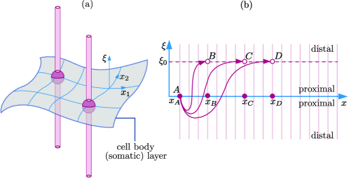
Figure 1: Schematic of the neural field model. (a) Dendrites are represented as unbranched fibres (red), orthogonal to a continuum of somas (somatic layer, in grey). (b) Model (1) is for a 1D somatic layer, with coordinate $x\in\mathbb{R}$, and fiber coordinate $\xi\in\mathbb{R}$. Input currents are generated in a small neighbourhood of the somatic layer, at $\xi=0$ and are delivered to a contact point, in a small neighbourhood of $\xi=\xi_{0}$. The strength of interaction depends on the distance between sources and contact points, measured along the somatic layer, hence the inputs that are generated at $A$ and transmitted to $B$, $C$, and $D$ depend on $|x_{B}-x_{A}|$, $|x_{C}-x_{A}|$, and $|x_{D}-x_{A}|$, respectively (see (2)).

This work introduces a computational method for approximating solutions to (1), subject to suitable initial and boundary conditions, and applies it to the numerical simulation of the model with kernel given by (2). Numerical methods for neural fields in 2-dimensional media have been introduced recently in flat geometries [16, 11, 12] and on 2-manifolds embedded in a 3-dimensional space [3, 21]. In addition, several available open-source codes, such as the Neural Field Simulator [13], the Brain Dynamics Toolbox [10], and NFTsim [18], perform simulations of neural field equations. Numerical schemes for models of type (1) have not been introduced, analysed, or implemented, and these are the main contributions of the present article.

In Section 2 we describe, analyse, and discuss implementation details of the numerical method. In Sections 3–4 we illustrate the performance of the method by means of some numerical experiments, including problems whose exact solution has known properties. The numerical results are discussed and their physical meaning is explained. We finish with some conclusions and discussion in Section 5.

2 Numerical Scheme

Numerical simulations are performed on (1), posed on a bounded, cylindrical somato-dendritic domain

$$\Omega=\mathbb{R}/2L_{x}\mathbb{Z}\times(-L_{\xi},L_{\xi}),$$

and subject to initial and boundary conditions,

(3) $$\partial_{t}V=(-\gamma+\nu\partial_{\xi\xi})V+K(V)+G \textrm{on $\Omega\times(0,T]$},$$

$$V({\mkern 2.0mu\cdot\mkern 2.0mu},{\mkern 2.0mu\cdot\mkern 2.0mu},0)=V_{0} \textrm{on $\Omega$},$$

$$\partial_{\xi}V({\mkern 2.0mu\cdot\mkern 2.0mu},-L_{\xi},{\mkern 2.0mu\cdot\mkern 2.0mu})=\partial_{\xi}V({\mkern 2.0mu\cdot\mkern 2.0mu},L_{\xi},{\mkern 2.0mu\cdot\mkern 2.0mu})=0 \textrm{on $(-L_{x},L_{x}]\times[0,T]$},$$

for some positive constants $T$, $L_{x}$, $L_{\xi}$. This setup implies $2L_{x}$-periodicity in the somatic direction, and Neumann boundary conditions in the dendritic direction. We denote by $K$ the integral operator defined by

$$(K(V))(x,\xi,t)=\int_{\Omega}W_{\Omega}(x,\xi,y,\eta)S(V(y,\eta,t))\mathop{}\!\mathrm{d}y\mathop{}\!\mathrm{d}\eta,\qquad(x,\xi)\in\Omega.$$

where $W_{\Omega}$ is the restriction of $W$ on $\Omega$. This restriction implies that the function $w$ in (2) be substituted by its periodic extension on $[-L_{x},L_{x})$. In the remainder of this paper we will omit the subscript $\Omega$ from $W$, and assume $w$ to be $2L_{x}$-periodic.

To expose our scheme we introduce a spatiotemporal discretisation using the evenly spaced grid $\{(x_{j},\xi_{i},t_{n})\}$ defined by

$$x_{j}=-L_{x}+jh_{x}, j\in\mathbb{N}_{n_{x}}, h_{x}=2L_{x}/n_{x},$$

$$\xi_{i}=-L_{\xi}+(i-1)h_{\xi}, i\in\mathbb{N}_{n_{\xi}}, h_{\xi}=2L_{\xi}/(n_{\xi}-1),$$

$$t_{n}=n\tau, n\in\mathbb{N}_{n_{t}}, \tau=T/n_{t},$$

where we posed $\mathbb{N}_{k}=\{1,2,\ldots,k\}$ for $k\in\mathbb{N}$. The scheme we propose uses the method of lines for (3), in conjunction with differentiation matrices for the diffusive term and a quadrature scheme for the integral operator.

Collocating (3) at the somato-dendritic nodes we obtain

(4) $$\begin{split}\partial_{t}V(x_{j},\xi_{i},t)=(-\gamma+\nu\partial_{\xi\xi})V(x_{j},\xi_{i},t)&+K(V)(x_{j},\xi_{i},t)\\ &+G(x_{j},\xi_{i},t)\quad(j,i)\in\mathbb{N}_{n_{x}}\times\mathbb{N}_{n_{\xi}},\end{split}$$

where, with a slight abuse of notation, we denote by $V$ an interpolant to the function $V$ in (3) through $\{(x_{j},\xi_{i})\}$. To obtain a numerical solution of the problem we must choose: (i) an approximation for the linear operator $(-\gamma+\nu\partial_{\xi\xi})$ at the somato-dendritic nodes; (ii) an approximation for the integral operator at the same nodes; (iii) a scheme to time step the derived set of ODEs.

In the presentation of the scheme, we shall use two equivalent representations for the voltage approximation: a matricial description

(5) $$V(t)=\{V_{ij}(t)\colon(i,j)\in\mathbb{N}_{n_{\xi}}\times\mathbb{N}_{n_{x}}\}\in\mathbb{R}^{n_{\xi}\times n_{x}},\qquad V_{ij}(t)\approx V(x_{j},\xi_{i},t),$$

and a lexicographic vectorial representation, obtained by introducing the index mapping $k(i,j)=n_{\xi}(i-1)+j$,

(6) $$U(t)=\{U_{k(i,j)}(t)\colon(i,j)\in\mathbb{N}_{n_{\xi}}\times\mathbb{N}_{n_{x}}\}\in\mathbb{R}^{n_{x}n_{\xi}}.$$

In the latter, we will sometimes suppress the dependence of $k$ on $(i,j)$, for notational convenience.

2.1 Discretisation of the linear operator

A simple choice for discretising the linear differential operator $(-\gamma+\nu\partial_{\xi\xi})$ is to adopt differentiation matrices [19]. If a differentiation matrix $D_{\xi\xi}\in\mathbb{R}^{n_{\xi}\times n_{\xi}}$ is chosen to approximate the action of the Laplacian operator $\partial_{\xi\xi}$ on twice differentiable, univariate functions defined on $[-L_{\xi},L_{\xi}]$, satisfying Neumann boundary conditions, and sampled at nodes $\{\xi_{i}\}$, then the action of the operator $-\gamma+\nu\partial_{\xi\xi}$ on bivariate functions defined on $[-L_{x},L_{x})\times[-L_{\xi},L_{\xi}]$, twice differentiable in $\xi$ with Neumann boundary conditions, sampled at the nodes $\{(x_{j},\xi_{i})\}$ with lexicographical ordering $k(i,j)$ is approximated by the following block-diagonal matrix

$$-\gamma I_{n_{x}n_{\xi}}+\nu I_{n_{x}}\otimes D_{\xi\xi}=\begin{bmatrix}-\gamma+\nu D_{\xi\xi}&&&\\ &-\gamma+\nu D_{\xi\xi}&&\\ &&\ddots&\\ &&&-\gamma+\nu D_{\xi\xi}\end{bmatrix},$$

where $I_{n}$, $n\in\mathbb{N}$, is the $n$-by-$n$ identity matrix, and $\otimes$ is the Kronecker product between matrices. Since the model prescribes diffusion only along the dendritic coordinate, the corresponding matrix has a block-diagonal structure with identical blocks, which can be exploited to improve performance in numerical computations. The sparsity pattern of a block is dictated by the underlying scheme to approximate the univariate Laplacian: we have full blocks if $D_{\xi\xi}$ is derived from spectral schemes, and sparse blocks for finite-difference schemes.

2.2 Discretisation of the nonlinear integral operator

The starting point to discretise the integral operator is an $m$th order quadrature formula with $q_{m}$ nodes $\{(y_{l},\eta_{l})\colon l\in\mathbb{N}_{q_{m}}\}$ and weights $\{\sigma_{l}\colon l\in\mathbb{N}_{q_{m}}\}$ for the integral of a bivariate function over $\Omega$,

$$Q(v)=\int_{\Omega}v(y,\eta)\,\mathop{}\!\mathrm{d}y\mathop{}\!\mathrm{d}\eta\approx\sum_{l\in\mathbb{N}_{m}}v(y_{l},\eta_{l})\sigma_{l}=Q_{m}(v).$$

Using this formula we approximate the nonlinear operator in (4) by

$$Q_{m}(K(V))(x_{j},\xi_{i},t)=\sum_{l\in\mathbb{N}{q_{m}}}W(x_{j},\xi_{i},y_{l},\eta_{l})S(V(y_{l},\eta_{l},t))\sigma_{l}.$$

We stress that, in general, the quadrature nodes $\{(y_{l},\eta_{l})\}$ and the collocation nodes $\{(x_{k(i,j)},\xi_{k(i,j)})\}$ are disjoint. The former are chosen so as to approximate accurately the integral term, the latter to approximate the differential operator. When the two grids are disjoint, an interpolation of $V$ with nodes $\{(y_{l},\eta_{l})\}$ is necessary to derive a set of ODEs at the collocation nodes. In the remainder of this paper we will assume that collocation and quadrature nodes coincide, so that we can omit the interpolant, for simplicity.

2.3 Matrix ODE formulation

Combining the differentiation matrix, the quadrature rule, and the lexicographic representation (6) we obtain a set of $n_{x}n_{\xi}$ ODEs

(7) $$\dot{U}(t) =(-\gamma I_{n_{x}n_{\xi}}+\nu I_{n_{x}}\otimes D_{\xi\xi})U(t)+F(U(t),t),$$

$$U(0) =U_{0}.$$

The structure of the differentiation matrix in section (2.1), however, suggests a rewriting of (7) in terms of the blocks of the linear operator, which correspond to “slices” at constant values of $x$: we recall the matrix representation (5) and obtain an equivalent matrix ODE formulation

(8) $$\dot{V}(t)=(-\gamma I_{n_{\xi}}+\nu D_{\xi\xi})V(t)+N(V(t))+G(t),$$

where $N$ is the matrix-valued function with components $N_{ij}(V)=Q_{m}(V)(x_{j},\xi_{i})$ and $G$ is the matrix with components $G(x_{j},\xi_{i},t)$. In passing, we note that the linear part of the equation involves a multiplication between an $n_{\xi}$-by-$n_{\xi}$ matrix and the $n_{\xi}$-by-$n_{x}$ matrix $V$.

2.4 Time-stepping scheme

The proposed time-stepping scheme for (3) is obtained from (8) with the following choices: (i) a first-order, implicit-explicit (IMEX) time-stepping scheme [1]; (ii) a second-order, centered finite-difference scheme for the differentiation matrix $D_{\xi\xi}$; (ii) a second-order trapezium rule for the quadrature rule $Q_{m}$. As we shall see, these choices bring a few computational advantages, which will be outlined below.

IMEX schemes treat the linear (diffusive) part of the ODE implicitly, and the nonlinear part explicitly, so that the stiff diffusive term is integrated implicitly to avoid excessively small time steps. The simplest IMEX method uses backward Euler for the diffusive term, leading to

(9) $$V^{0} =V_{0},$$

$$AV^{n} =V^{n-1}+\tau N(V^{n-1})+\tau G^{n-1},\qquad n\in\mathbb{N},$$

where $V^{n}\approx V(t_{n})$, $G^{n}=G(t_{n})$, and $A$ is the matrix

(10) $$A=(1+\gamma\tau)I_{n_{\xi}}-\tau\nu D_{\xi\xi}.$$

In concrete calculations we use second-order centred finite differences, leading to

(11) $$D_{\xi\xi}=\Delta/h_{\xi}^{2},\qquad\Delta=\begin{bmatrix}-2&2&&&&\\ 1&-2&1&&&\\ &\ddots&\ddots&\ddots&&\\ &&1&-2&1&\\ &&&2&-2&\end{bmatrix},$$

in which Neumann boundary conditions are included in the differentiation matrix.

Finally, we discuss the choice of the quadrature scheme. We use a composite trapezium scheme with nodes $\{x_{j}\}$ and weights $\{\rho_{j}\}$ in $x$, and nodes $\{\xi_{i}\}$ and weights $\{\sigma_{i}\}$ in $\xi$, respectively, hence quadrature and collocation sets coincide,

(12) $$N_{ij}(V)=\sum_{j^{\prime}\in\mathbb{N}{n_{x}}}\sum_{i^{\prime}\in\mathbb{N}{n_{\xi}}}W(x_{j},\xi_{i},x_{j^{\prime}},\xi_{i^{\prime}})S(V_{i^{\prime},j^{\prime}})\rho_{j^{\prime}}\sigma_{i^{\prime}}.\quad(i,j)\in\mathbb{N}_{n_{\xi}}\times\mathbb{N}_{n_{x}}.$$

2.5 Properties of the IMEX scheme

In this section we collect some analytical results on the IMEX scheme (9)–(12). We work with spaces of sufficiently regular continuous functions, which provides the simplest setting for our results. We denote by $C^{k}(D)$ the space of $k$-times continuously differentiable functions from $D$ to $\mathbb{R}$, where $k$ is an integer, $D$ a domain in $\mathbb{R}^{3}$. We also indicate by $C_{b}^{k}(D)$ the space of continuous functions from $D$ to $\mathbb{R}$ with bounded and continuous partial derivatives up to order $k$. Both spaces are endowed with the infinity norm $\|{\mkern 2.0mu\cdot\mkern 2.0mu}\|_{\infty}$. We will use the symbol $|{\mkern 2.0mu\cdot\mkern 2.0mu}|_{\infty}$ for the standard infinity-norm on matrices, induced by the corresponding vector norm. In addition, we will denote by $\bar{D}$ the closure of $D$.

We begin with a generic assumption of boundedness on the functions in (3): There exist $C_{W},C_{S},C_{G}>0$ such that

$$|W|\leq C_{W}\;\textrm{in $\Omega\times\Omega$},\qquad|S|\leq C_{S}\;\textrm{in $\mathbb{R}$},\qquad|G|\leq C_{G}\;\textrm{in $\Omega\times\mathbb{R}$}.$$

Lemma 2.1 (Boundedness of IMEX solution).

Assume Hypothesis 2.5, then there exists a unique bounded sequence $(V^{n})_{n\in\mathbb{N}}$ satisfying the IMEX scheme (9)–(12). In addition, the following bound holds

$$|V^{n}|_{\infty}\leq|V^{0}|_{\infty}+n_{x}\frac{\mu(\bar{\Omega})C_{W}C_{S}+C_{G}}{\gamma},\qquad n\in\mathbb{N}.$$

Proof 2.2.

The matrix $A$ in (10) has real, strictly positive eigenvalues given by

$$\lambda_{k}=1+\gamma\tau+\frac{4\nu\tau}{h_{\xi}^{2}}\bigg{[}\sin\bigg{(}\frac{\pi(k-1)}{2n_{\xi}}\bigg{)}\bigg{]}^{2},\qquad k\in\mathbb{N}_{n_{\xi}},$$

where we have used the fact that the eigenvalues of $D_{\xi\xi}$ are known in closed form. We conclude that $A$ is invertible, hence for any fixed $n\in\mathbb{N}$, the matrix $V^{n}$ solving (9) is unique. In addition, $A$ is strictly diagonally dominant, hence the following bound holds [20]

(13) $$|A^{-1}|_{\infty}\leq\max_{i\in\mathbb{N}_{\xi}} \frac{1}{|A_{ii}|-\sum_{j\neq i}|A_{ij}|}=\frac{1}{1+\gamma\tau}.$$

To prove boundedness of the sequence $(V^{n})_{n\in\mathbb{N}}$ we first bound the matrices $N(V^{n-1})$, $G^{n}$ appearing in (9)

$$\begin{aligned} |N(V^{n-1})|_{\infty}&=\max_{i\in\mathbb{N}_{n_{\xi}}}\sum_{j\in\mathbb{N}_{n_{x}}}|N_{ij}(V^{n-1})|\\ &\leq\max_{i\in\mathbb{N}_{n_{\xi}}}\sum_{j\in\mathbb{N}_{n_{x}}}\sum_{j^{\prime}\in\mathbb{N}{n_{x}}}\sum_{i^{\prime}\in\mathbb{N}{n_{\xi}}}|W(x_{j},\xi_{i},x_{j^{\prime}},\xi_{i^{\prime}})S(V_{i^{\prime},j^{\prime}})\rho_{j^{\prime}}\sigma_{i^{\prime}}|\\ &\leq C_{W}C_{S}\max_{i\in\mathbb{N}_{n_{\xi}}}\sum_{j\in\mathbb{N}_{n_{x}}}\sum_{j^{\prime}\in\mathbb{N}{n_{x}}}\sum_{i^{\prime}\in\mathbb{N}{n_{\xi}}}\rho_{j^{\prime}}\sigma_{i^{\prime}}\\ &\leq C_{W}C_{S}\max_{i\in\mathbb{N}_{n_{\xi}}}\sum_{j\in\mathbb{N}_{n_{x}}}\mu(\bar{\Omega})=n_{x}\mu(\bar{\Omega})C_{W}C_{S},\end{aligned},$$

and similarly $|G^{n-1}|_{\infty}\leq n_{x}C_{G}$, and then combine them with the bound for $|A^{-1}|_{\infty}$ to find

$$|V^{n}|_{\infty} \leq|A^{-1}|_{\infty}\Big{(}|V^{n-1}|_{\infty}+\tau|N(V^{n-1})|_{\infty}+\tau|G^{n-1}|_{\infty}\Big{)}$$

$$\leq\frac{1}{1+\gamma\tau}\Big{(}|V^{n-1}|_{\infty}+\tau n_{x}\mu(\bar{\Omega})C_{W}C_{S}+\tau n_{x}C_{G}\Big{)}.$$

We set

$$r=\frac{1}{1+\gamma\tau}<1,\qquad q=\frac{\tau n_{x}}{1+\gamma\tau}(\mu(\bar{\Omega})C_{W}C_{S}+C_{G}),$$

and use induction and elementary properties of the geometric series to obtain

$$|V^{n}|_{\infty}\leq r^{n}|V^{0}|_{\infty}+q\sum_{j=0}^{n-1}r^{j}\leq|V^{0}|_{\infty}+\frac{q}{1-r},$$

which proves the assertion.

In addition to proving boundedness of the solution, we address the convergence rate of the IMEX scheme. For this result, we assume the existence of a sufficiently regular solution to (3).

Lemma 2.3 (Local convergence rate of the IMEX scheme).

Assume Hypothesis 2.5, $W\in C^{2}(\Omega\times\Omega)$, $S\in C^{2}_{b}(\Omega)$, and assume (3) admits a strong solution $V_{*}$ whose partial derivatives $\partial_{tt}V_{*}$, $\partial_{xx}V_{*}$, $\partial_{x\xi}V_{*}$, $\partial_{\xi\xi}V_{*}$, $\partial_{\xi\xi\xi\xi}V_{*}$ exist and are bounded on $\bar{\Omega}\times[0,T]$. Denote by $V^{n}_{*}$ the matrix with elements $(V_{*}^{n})_{ij}=V_{*}(x_{j},\xi_{i},t_{n})$, for $(i,j,n)\in\mathbb{N}_{n_{x}}\times\mathbb{N}_{n_{\xi}}\times\mathbb{N}_{n_{t}}$. Further, let $(V^{n})_{n\in\mathbb{N}}$ be the solution to the IMEX scheme (9)–(12), and let

$$\zeta=n_{x}\mu(\bar{\Omega})\|W\|_{\infty}\|S^{\prime}\|_{\infty},\qquad h=\max(h_{\xi},h_{x}).$$

There exist constants $C_{\tau},C_{h}>0$ such that

(14) $$|V^{n}-V_{*}^{n}|_{\infty}\leq\frac{1}{\gamma-\zeta}(C_{\tau}\tau+C_{h}h^{2}) \text{if $\zeta<\gamma$},$$

(15) $$|V^{n}-V_{*}^{n}|_{\infty}\leq\frac{T}{1+\gamma\tau}(C_{\tau}\tau+C_{h}h^{2}) \text{if $\zeta=\gamma$},$$

(16) $$|V^{n}-V_{*}^{n}|_{\infty}\leq\frac{C_{\tau}\tau+C_{h}h^{2}}{\zeta-\gamma}\exp\frac{(\zeta-\gamma)T}{1+\gamma\tau} \text{if $\zeta>\gamma$}.$$

Proof 2.4.

The regularity assumptions on $V_{*}$, and standard results on finite-difference approximation and trapezium quadrature rule guarantee the existence of constants $C_{tt},C_{xx},C_{\xi\xi},C_{\xi\xi\xi\xi}>0$ such that for all $n\in\{0\}\cup\mathbb{N}_{n_{t}}$

(17) $$AV_{*}^{n}=V_{*}^{n-1}+\tau\big{(}N(V_{*}^{n-1})+G^{n-1}+C_{tt}\tau+C_{\xi\xi\xi\xi}h^{2}_{\xi}+C_{xx}h_{x}^{2}+C_{\xi\xi}h_{\xi}^{2}\big{)},$$

where the errors for the forward finite-difference in $t$, centred finite-difference in $\xi$, and trapezium rule are listed progressively, with constants proportional to the respective partial derivatives. We subtract (17) from

$$AV^{n}=V^{n-1}+\tau N(V^{n-1})+\tau G^{n-1},$$

and obtain the error bound

(18) $$|V-V_{*}^{n}|_{\infty}\leq|A^{-1}|_{\infty}\big{(}|V-V_{*}^{n}|_{\infty}+\tau|N(V^{n})-N(V_{*}^{n})|_{\infty}+\tau\omega\big{)},$$

where $\omega=C_{\tau}\tau+C_{h}h^{2}$, $C_{\tau}=C_{tt}$, $C_{h}=\max(C_{xx},C_{\xi\xi},C_{\xi\xi\xi\xi})$, and $h=\max(h_{\xi},h_{x})$. Since the first derivative $S^{\prime}$ of $S$ is bounded, we have the following estimate for the nonlinear term

$$|N(V^{n})-N(V_{*}^{n})|_{\infty} \leq\|W\|_{\infty}\|S^{\prime}\|_{\infty}\max_{i\in\mathbb{N}_{n_{\xi}}}\sum_{j\in\mathbb{N}_{n_{x}}}\sum_{j^{\prime}\in\mathbb{N}{n_{x}}}\sum_{i^{\prime}\in\mathbb{N}{n_{\xi}}}|V^{n}_{i^{\prime}j^{\prime}}-(V_{*}^{n})_{i^{\prime}j^{\prime}}|\rho_{j^{\prime}}\sigma_{i^{\prime}}$$

$$\leq n_{x}\mu(\bar{\Omega})\|W\|_{\infty}\|S^{\prime}\|_{\infty}|V^{n}-V_{*}^{n}|_{\infty}$$

$$=\zeta|V^{n}-V_{*}^{n}|_{\infty},$$

which, together with (13) and (18) gives a recursive bound for the $\infty$-norm matrix error $|V^{n}-V_{*}^{n}|_{\infty}$,

$$E^{0}=0,\qquad E^{n}\leq\frac{1+\zeta\tau}{1+\gamma\tau}E^{n-1}+\frac{\tau\omega}{1+\gamma\tau}:=rE^{n-1}+q.\qquad n\in\mathbb{N}_{n_{t}}.$$

Hence,

(19) $$E^{n}\leq q\frac{r^{n}-1}{r-1},\quad r\neq 1,\qquad E^{n}\leq nq\quad r=1,\qquad n\in\mathbb{N}_{n_{t}}.$$

If $\zeta<\gamma$, then $r<1$, and we obtain (14) as

$$E^{n}\leq\frac{q}{1-r}=\frac{\omega}{\gamma-\zeta}=\frac{1}{\gamma-\zeta}(C_{\tau}\tau+C_{h}h^{2}),\qquad n\in\mathbb{N}_{n_{t}}.$$

If $\zeta=\gamma$, then $r=1$ and (15) is found as follows

$$E^{n}\leq nq\leq\frac{n_{t}\tau\omega}{1+\gamma\tau}=\frac{T}{1+\gamma\tau}(C_{\tau}\tau+C_{h}h^{2}),\qquad n\in\mathbb{N}_{n_{t}}.$$

If $\zeta>\gamma$, then $r>1$ and we can bound the $n$th term of the sequence with an exponential, using the bound $(1+x/n)^{n}\leq\operatorname{e}^{x}$ for all $x\in\mathbb{R}$, as follows,

$$r^{n}=\bigg{(}1+\frac{(\zeta-\gamma)n\tau}{n(1+\gamma\tau)}\bigg{)}^{n}\leq\exp\frac{(\zeta-\gamma)n\tau}{1+\gamma\tau}\leq\exp\frac{(\zeta-\gamma)T}{1+\gamma\tau},$$

which combined with (19) gives (16):

$$E^{n}\leq\frac{\omega}{\zeta-\gamma}\exp\frac{(\zeta-\gamma)T}{1+\gamma\tau}=\frac{C_{\tau}\tau+C_{h}h^{2}}{\zeta-\gamma}\exp\frac{(\zeta-\gamma)T}{1+\gamma\tau}.$$

The preceding lemma shows that the IMEX scheme has first order convergence in time, and second order convergence in space. As expected, this conclusion holds without imposing any restriction to the size of $\tau$ in relation to $h$, as happens, for example, in the case of explicit methods for parabolic equations. In passing we note that if $\zeta<\gamma$ and $V_{*}(t)$ exists for all $t\in\mathbb{R}$, the error estimate (14) holds for $n\in\mathbb{N}$, that is, in an unbounded interval of time; on the other hand, the error estimates do not hold on an unbounded time interval when $\zeta\geq\gamma$, as the bounds depend on $T$.

2.6 Implementational aspects and efficiency

In this section we make a few considerations on the implementation of the proposed IMEX scheme, with the view of comparing its efficiency to an ordinary IMEX scheme, that is, to an IMEX scheme applied to (7).

2.6.1 Implementation

IMEX schemes for planar semilinear problems require the inversion of a discretised Laplacian, which usually is a square matrix with the same dimension of the problem ($n_{\xi}n_{x}$ equations in our case). The particular structure of the problem under consideration, however, implies that the matrix to be inverted is much smaller (the square matrix $A$ has only $n_{\xi}$ rows and $n_{\xi}$ columns). At each time step (9) we solve a problem of the type $AX=B$, where $A\in\mathbb{R}^{n_{\xi}\times n_{\xi}}$, and $X,B\in\mathbb{R}^{n_{\xi}\times n_{x}}$. This can be achieved efficiently by pre-computing a factorisation of $A$, and then back-substituting for all columns of $B$. Since the matrix $A$ is sparse and with low bandwidth, efficient implementations of the $LU$ decompositions and backsubstitution can be used to solve the $n_{x}$ linear problems corresponding to the columns of $X$ and $B$.

An important aspect of the numerical implementation is the evaluation of the nonlinear term (12): evaluating the right-hand side of (9) requires in general $O(n^{2}_{\xi}n^{2}_{x})$ operations, which is a bottleneck for the time stepper, in particular for large domains. However, the structure of the problem can be exploited once again to evaluate this term efficiently. We make use of the following properties:

1. The kernel $W$ specified in (2) has a product structure, hence

   $$W(x_{j},\xi_{i},x_{j^{\prime}},\xi_{i^{\prime}})=\alpha_{i}\alpha^{\prime}_{i^{\prime}}w(|x_{j}-x_{j^{\prime}}|).$$

   where $\alpha_{i}=\delta_{\varepsilon}(\xi_{i}-\xi_{0})$, $\alpha^{\prime}_{i^{\prime}}=\delta_{\varepsilon}(\xi_{i^{\prime}})$. In addition, $w$ is periodic, therefore the matrix with entries $w(|x_{j}-x_{j^{\prime}}|)$ is circulant with (rotating) row vector $w=\{w(|x_{j}|)\colon j\in\mathbb{N}_{n_{x}}\}\in\mathbb{R}^{1\times n_{x}}$.

2. The function $x\mapsto V(x,{\mkern 2.0mu\cdot\mkern 2.0mu})$ is $2L_{x}$-periodic, hence the trapezium rule has identical weights $\rho_{j}=h_{x}$, and the integration in $x$ is a circular convolution, which can be performed efficiently in $O(n_{x}\log n_{x})$ operations, using the Discrete Fourier Transform (DFT).

We have

(20) $$N_{ij}(V)=\alpha_{i}\sum_{j^{\prime}\in\mathbb{N}_{n_{x}}}w_{j-j^{\prime}}\rho_{j^{\prime}}\sum_{i^{\prime}\in\mathbb{N}_{n_{\xi}}}\alpha^{\prime}_{i^{\prime}}\sigma_{i^{\prime}}S(V_{i^{\prime}j^{\prime}})\qquad(i,j)\in\mathbb{N}_{n_{\xi}}\times\mathbb{N}_{n_{x}},$$

and a DFT can be used to perform the outer sums [8, 16]. Introducing the direct, $\mathcal{F}_{n}$, and inverse, $\mathcal{F}_{n}^{-1}$, DFTs for $n$-vectors, we express compactly the nonzero elements of $N$ as follows

(21) $$N=\alpha h_{x}\mathcal{F}^{-1}_{n_{x}}\big{[}\mathcal{F}_{n_{x}}[w]\odot\mathcal{F}_{n_{x}}[(\alpha^{\prime}\odot\sigma)^{T}S(V)]\big{]},$$

where $\alpha,\alpha^{\prime},\sigma\in\mathbb{R}^{n_{\xi}\times 1}$ are column vectors, and $\odot$ denotes the Hadamard product, that is, elementwise vector multiplication. The formula above evaluates the nonlinear term $N$ in just $O(n_{x}n_{\xi})+O(n_{x}\log n_{x})$ operations.

We summarise our implementation with the pseudocode provided in Algorithm 1, and we will henceforth compare quantitatively its efficiency with a standard IMEX implementation, which we also provide in Algorithm 2. The matricial version, Algorithm 1 exposes row- and column-vectors, for which a very compact Matlab implementation can be derived. We give an example of such implementation in Appendix A, and we refer the reader to [2] for a repository of codes used in this article.

2.6.2 Efficiency estimates

We now make a few considerations about the efficiency of our algorithm. We will provide two main measures of efficiency: an estimate of the floating point operations (flops), and an estimate of the storage space (in floating point numbers) required by the algorithm, as a function of the input data which, in our case, are the number of gridpoints in each direction, $n_{x}$ and $n_{\xi}$. We are interested in how the estimates scale for large $n_{x},n_{\xi}$.

To estimate the number of flops, we count the number of operations required by Algorithms 1 and 2 in the initialisation step (lines 2–6), and in a single time step (lines 8–12). We base our estimates on the following facts and hypotheses:

1. The cost of multiplying an $m$-by-$n$ matrix by an $n$-vector is $2mn-m$ flops.

2. If an $n$-by-$n$ matrix is tridiagonal, then the matrices $L$ and $U$ of its $LU$-factorisation are bidiagonal, and $L$ has $1$ along its main diagonal. This implies that storing the $LU$ factorisation requires only $3$ $n$-vectors. Calculating the $LU$ factorisation costs $2n+1$ flops, while solving the corresponding linear problem $LUx=b$, with $x,b\in\mathbb{R}^{n}$, requires $2n-2$ and $3n-2$ flops for the forward- and backward-subsitution, respectively. Similar considerations apply if $A$ is not tridiagonal, but still sparse, as it would be obtained using a different discretisation method for the diffusive operator: estimates for the flops of the corresponding $PLU$-factorisation depend, in general, on the sparsity pattern of $A$, as well as on the permutation strategy, which is heuristic but can have an impact on the sparsity of $L$ and $U$, thereby influencing the performance of the algorithm. We present calculations only in the case of a tridiagonal matrix $A$, for which explicit estimates are possible.

3. As stated above, it is well known that a single FFT of an $n$-vector costs $O(n\log n)$ operations.

4. We assume that function evaluations of the functions $G$, $S$, $w$, $\delta$ cost one flop. This estimate is optimistic, as most function evaluations will require more than one flop, but we make this simplifying assumption for both the algorithms we are comparing.

1

Input : Initial condition $V^{0}\in\mathbb{R}^{n_{\xi}\times n_{x}}$, time step $\tau$, number of steps $n_{t}$.

Output : An approximate solution $(V^{n})_{n=1}^{n_{t}}\subset\mathbb{R}^{n_{\xi}\times n_{x}}$

2 begin

3      Compute grid vectors $\xi\in\mathbb{R}^{n_{\xi}\times 1}$, $x\in\mathbb{R}^{1\times n_{x}}$.

4      Compute synaptic vectors $w,\hat{w}=\mathcal{F}_{n_{x}}[w]\in\mathbb{R}^{1\times n_{x}}$.

5      Compute synaptic vectors $\alpha,\alpha^{\prime}\in\mathbb{R}^{n_{\xi}\times 1}$.

6      Compute quadrature weights $\sigma\in\mathbb{R}^{n_{\xi}\times 1}$.

7      Compute sparse $LU$-factorisation of $A$,

$$LU=A\in\mathbb{R}^{n_{\xi}\times n_{\xi}}.$$

8      for $n=1,\ldots,n_{t}$ do

9           Set $V=V^{n-1}\in\mathbb{R}^{n_{\xi}\times n_{x}}$.

10           Compute the external input at time $t_{n-1}$ and store it in $G\in\mathbb{R}^{n_{\xi}\times n_{x}}$.

11           Set $z=\mathcal{F}_{n_{x}}\big{[}(\alpha^{\prime}\odot\sigma)^{T}S(V)\big{]}\in\mathbb{R}^{1\times n_{x}}$.

12           Set $N=h_{x}\alpha\mathcal{F}^{-1}_{n_{x}}[\hat{w}\odot z]\in\mathbb{R}^{n_{\xi}\times n_{x}}$.

13           Solve for $V^{n}$ the linear problem $(LU)V^{n}=V+\tau(N+G)$.

14           end for

15          

16           end

17          

Algorithm 1 IMEX time stepper in matrix form (8), nonlinear term computed with pseudospectral evaluation (21)

1

Input : Initial condition $U^{0}\in\mathbb{R}^{n_{\xi}n_{x}}$, time step $\tau$, number of steps $n_{t}$.

Output : An approximate solution $(U^{n})_{n=1}^{n_{t}}\subset\mathbb{R}^{n_{\xi}n_{x}}$

2 begin

3      Compute grid vectors $\xi\in\mathbb{R}^{n_{\xi}}$, $x\in\mathbb{R}^{n_{x}}$.

4      Compute synaptic vector $w\in\mathbb{R}^{1\times n_{x}}$.

5      Compute synaptic vectors $\alpha,\alpha^{\prime}\in\mathbb{R}^{n_{\xi}\times 1}$.

6      Compute quadrature weights $\rho\in\mathbb{R}^{n_{x}}$, $\sigma\in\mathbb{R}^{n_{\xi}}$.

7      Compute sparse $LU$-factorisation

$$LU=\big{(}(1+\tau\gamma)I_{n_{x}n_{\xi}}-\tau\nu I_{n_{x}}\otimes D_{\xi\xi}\big{)}\in\mathbb{R}^{n_{\xi}n_{x}\times n_{\xi}n_{x}}.$$

for $n=1,\ldots,n_{t}$ do

8           Set $Z=U^{n-1}\in\mathbb{R}^{n_{\xi}n_{x}}$.

9           Compute the external input at time $t_{n-1}$ and store it in $G\in\mathbb{R}^{n_{\xi}n_{x}}$.

10           Compute the nonlinear term $N$ using (12).

11           Solve for $U^{n}$ the linear problem $(LU)U^{n}=Z+\tau(N+G)$.

12           end for

13          

14           end

15          

Algorithm 2 IMEX time stepper in vector form (7), nonlinear term evaluated with quadrature formula (12).

In Table 1 we count flops required in each line of Algorithms 1 and 2. The data is grouped so as to distinguish between the initialisation phase of the algorithms, and the iterations for the time steps. Algorithm 1 outperforms substantiatlly Algorithm 2 in both phases. In the initialisation, the number of flops scales linearly for Algorithm 1, and quadratically for Algorithm 2. This is mostly owing to the $LU$-factorisation step, which involves the $n_{\xi}$-by-$n_{\xi}$ matrix $A$ in the former, and an $n_{\xi}n_{x}$-by-$n_{\xi}n_{x}$ matrix in the latter.

The efficiency gain is more striking in the cost per time step: owing to the pseudospectral evaluation of the nonlinearity, only $O(n_{\xi}n_{x})+O(n_{x}\log n_{x})$ flops are necessary in Algorithm 1, as opposed to $O(n^{2}_{\xi}n^{2}_{x})$ flops in Algorithm 2.

Table 1: Flop count for the initialisation step (lines 2–6) and for one time step (lines 8–12) in Algorithms 1,2.

Algorithm 1		Algorithm 2
Lines	Flops	Lines	Flops
2	$n_{\xi}+n_{x}$	2	$n_{\xi}+n_{x}$
3	$2n_{x}$	3	$n_{x}$
4	$2n_{\xi}$	4	$2n_{\xi}$
5	$n_{\xi}$	5	$n_{\xi}+n_{x}$
6	$2n_{\xi}-1$	6	$2n_{\xi}n_{x}-1$
2–6	$O(n_{\xi})+O(n_{x})$	2–6	$O(n_{\xi}n_{x})$
8	$n_{\xi}n_{x}$	8	$n_{\xi}n_{x}$
9	$n_{\xi}n_{x}$	9	$n_{\xi}n_{x}$
10	$3n_{\xi}n_{x}+O(n_{x}\log n_{x})+n_{\xi}-n_{x}$	10	$2n^{2}_{\xi}n_{x}^{2}-n^{2}_{\xi}n_{x}$
11	$n_{\xi}n_{x}+O(n_{x}\log n_{x})+2n_{x}$	11	$5n_{\xi}n_{x}-4$
12	$5n_{\xi}n_{x}-4n_{x}$
8–12	$O(n_{\xi}n_{x})+O(n_{x}\log n_{x})$	8–11	$O(n^{2}_{\xi}n^{2}_{x})$

Table 2: Space requirements, measured in Floating Point Numbers, for Algorithms 1 and 2. Arrays $d_{1},\ldots,d_{3}$, store diagonals of the $LU$-factorisation in the respective algorithms.

Floating Point Numbers	Algorithm 1	Algorithm 2
$n_{\xi}$	$\xi,\alpha,\alpha^{\prime},d_{1},d_{2},d_{3},z$	$\xi,\rho,\alpha,\alpha^{\prime}$
$n_{x}$	$x,w,\sigma$	$x,\sigma,w$
$n_{\xi}n_{x}$	$V,V^{n},G,N$	$U^{n},Z,N,G,d_{1},d_{2},d_{3}$
Total	$4n_{x}n_{\xi}+7n_{\xi}+3n_{x}$	$7n_{x}n_{\xi}+2n_{\xi}+2n_{x}$

An important point to note that, in the case of a 2D somatic space with, say coordinates $(x,y,\xi)$ and $n_{x}=n_{y}=N$, $n_{\xi}$ grid points (see Figure 1(a)), the size of the matrix $A$ in Algorithm 1 remains unaltered, while Algorithm 2 requires the factorisation and inversion of a much larger matrix, of size $n_{\xi}N^{2}$-by-$n_{\xi}N^{2}$. Estimates for the efficiencies in this case can be obtained by replacing $n_{x}$ by $N^{2}$ in the table, leading to much greater savings.

Finally, in Table 2 we collect the variables used by both algorithms, and count the storage requirement of each of them, measured floating point numbers. The results show that Algorithm 1 requires asymptotically the same storage as Algorithm 2 $O(n_{\xi}n_{x})$. For fixed values of $n_{\xi}$ and $n_{x}$, however, the latter uses almost twice as much storage space as the former.

3 Travelling waves

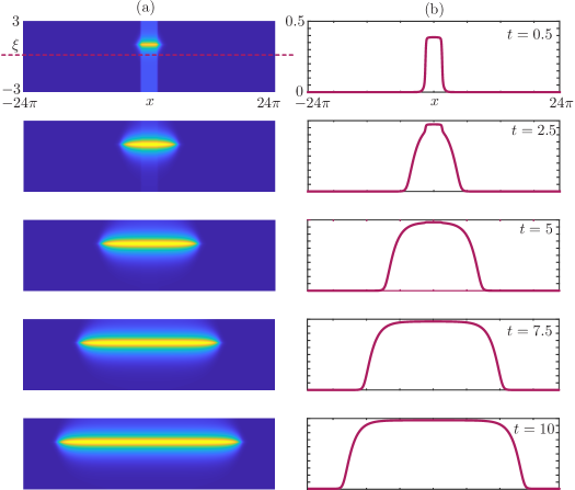
Figure 2: Coherent structure observed in time simulation of (3), (22), (23). (a): Pseudocolor plot of $V(x,\xi,t)$ at several time points, showing two counter-propagating waves. (b): Solution at $\xi=0$, showing the wave profile. Parameters: $\xi_{0}=1$, $\varepsilon=0.005$, $\nu=0.4$, $\gamma=1$, $\beta=1000$, $\theta=0.01$, $\kappa=3$, $L_{x}=24\pi$, $L_{\xi}=3$, $n_{x}=2^{10}$, $n_{\xi}=2^{12}$, $\tau=0.05$.

We tested the algorithm on an analytically tractable neural field problem, and we report in this section our numerical experiments. For the test, we take a sigmoidal firing rate function

(22) $$S(V)=\frac{1}{1+\exp(-\beta(V-\theta))},$$

and kernel specified by

(23) $$w(x)=\frac{\kappa}{2}\exp\bigg{(}-\frac{|x|}{2}\bigg{)},\qquad\delta_{\varepsilon}(\xi)=\frac{1}{\varepsilon\sqrt{\pi}}\exp\bigg{(}-\frac{\xi^{2}}{\varepsilon^{2}}\bigg{)}$$

where $\beta,\theta,\kappa$ are positive constants. If $S(V)=H(V-\theta)$, $H$ being the Heaviside function, $\delta_{\varepsilon}$ is replaced by the Dirac delta distribution, and the evolution equation is posed on $\mathbb{R}^{2}$, then the model supports solutions for which $V(x,0,t)$ is a travelling front $V(x,0,t)=\varphi(x-v_{*}t)$, with $\varphi(\pm\infty)=V_{\pm}$, whose speed $v_{*}$ satisfies the implicit equation [17]

(24) $$\frac{\kappa\exp(-\psi(v_{*},\nu)\xi_{0})}{2\psi(v_{*},\nu)\nu}-\theta=0,\qquad\psi(v_{*},\nu)=\sqrt{\frac{\gamma+v_{*}}{\nu}}.$$

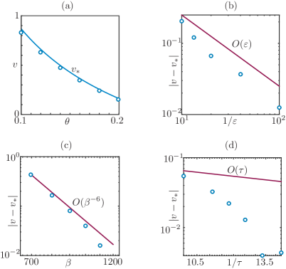
Figure 3: (a) Travelling wave speed versus firing rate threshold, computed analytically via (24), and numerically via the time-stepper. (b)–(d) Convergence of the computed speed to the analytical speed at $\theta=0.01$, as a function of the the kernel support parameter $\varepsilon$, the steepness of the sigmoid $\beta$, and the time-stepping parameter $\tau$, respectively. Parameters as in (2).

To test our scheme we study solutions to (3), (22), (23) with $L_{x},\beta\gg 1$, $L_{\xi}\gg\sqrt{\nu/\gamma}$, (the characteristic electrotonic length), and $\varepsilon\ll 1$. Since for this problem $[-L_{x},L_{x})\cong\mathbb{S}$, we expect to observe at $\xi=\xi_{0}$ two counter-propagating waves with approximate speed $v$ and

$$V(\pm L_{x},\xi_{0},t)\approx V_{+},\qquad V(0,\xi_{0},t)\approx V_{-}.$$

We show an exemplary profile of this coherent structure in Figure 2, where we observe two counter-propagating waves, as described above.

Since the wavespeed $v_{*}$ is available implicitly, we performed some tests to validate the proposed algorithm. Firstly, we compute roots of (24) in the variable $v_{*}$, as a function of the firing rate threshold $\theta$. In Figure 3(a) we observe a good agreement with the wavespeed observed in direct simulations. The latter has been computed by post-processing data from numerical simulations: using first-order interpolants we approximate a positive function $x_{*}(t)$ such that $V(x_{*}(t),0,t)=\theta$, that is, the $\theta$-level set of $V(x,0,t)$ on $[0,L_{x}]\times[0,T]$; after an initial transient, $\dot{x}_{*}(t)$ is approximately constant and provides an estimate of $v_{*}$, which is derived via first-order finite differences. In Figure 3(a) we observe a small discrepancy, which should be expected as we have several sources of error, namely: the time-stepping error, the spatial discretisation error for the differential and integral operators, the error due to the sigmoidal firing rate and to $\delta_{\varepsilon}$ (the theory is valid for Heaviside firing rate and for a Dirac-delta distribution $\delta$). In Figures 3(b)–(d) we show convergence plots for these errors (except for the second-order spatial discretisation error which is dominated in numerical simulations by the first-order time-stepping error).

4 Turing instability

The model defined by (1), with an appropriate choice of somatic interaction, can also support a Turing instability to spatially periodic patterns [4]. These in turn may either be independent of time or periodic in time. In the latter case this leads to periodic travelling waves. Whether emergent patterns be static or dynamic they both provide another validation test for the numerical scheme presented here, as the bifurcation point as determined analytically from a Turing analysis should agree with the onset of patterning in a direct numerical simulation. A relatively recent description of the method for determining the Turing instability in a neural field with dendritic processing can be found in [7]. Here we briefly summarise the necessary steps to arrive at a formula for the continuous spectrum, from which the Turing instability can be obtained.

In general a homogeneous steady state solution of (1) will only exist if either $S(0)=0$ or $\int_{\mathbb{R}^{2}}W(x,\xi,y,\eta)\mathop{}\!\mathrm{d}y\mathop{}\!\mathrm{d}\eta=\text{constant}$ for all $(x,\xi)$. The latter condition is not generic, and so for the purposes of this validation exercise we shall work with the choice $S(0)=0$ for which $V=0$ is the only homogeneous steady state. Linearising around $V=0$ and using (2) gives an evolution equation for the perturbations $\delta V(x,\xi,t)$ that can be written in the form

(25) $$\delta V(x,\xi,t)=S^{\prime}(0)\int_{-\infty}^{t}\Theta(\xi-\xi_{0},t-s)\int_{\mathbb{R}}w(|x-x^{\prime}|)\delta V(x^{\prime},0,s)\mathop{}\!\mathrm{d}x^{\prime}\mathop{}\!\mathrm{d}s,$$

where

$$\Theta(\xi,t)=\mathrm{e}^{-\gamma t}\frac{\mathrm{e}^{-\xi^{2}/(4\nu t)}}{\sqrt{4\pi\nu t}}H(t).$$

Focusing on a somatic field $\delta V(x,0,t)$, we see from (25) (with $\xi=0$) that this has solutions of the form $\operatorname{e}^{\lambda t}\operatorname{e}^{ipx}$ for $\lambda\in\mathbb{C}$ and $p\in\mathbb{R}$, where $\lambda=\lambda(p)$ is defined by the implicit solution of $\mathcal{E}(\lambda,p)=0$, where

(26) $$\mathcal{E}(\lambda,p)=1-S^{\prime}(0)\frac{\exp(-\psi(\lambda,\nu)\xi_{0})}{2\psi(\lambda,\nu)\nu}\widehat{w}(p).$$

Here the function $\psi$ is defined as in (24) and $\widehat{w}(p)$ is the Fourier transform of $w$:

(27) $$\widehat{w}(p)=\int_{\mathbb{R}}w(|y|)\operatorname{e}^{-ipy}\mathop{}\!\mathrm{d}y.$$

We note that since $w(x)=w(|x|)$ then $\widehat{w}(p)\in\mathbb{R}$.

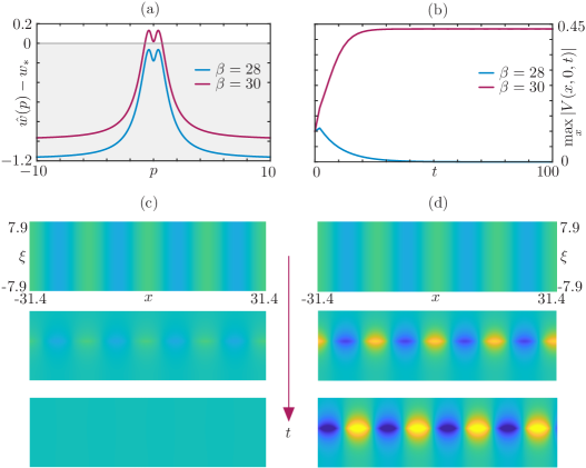
Figure 4: Numerical simulation of Turing bifurcation for the model with kernel and firing rate function given in (28). (a): Plots of $\hat{w}(p)-w_{*}$ for $\beta=28$ and $\beta=30$, from which we deduce that a Turing bifurcation occurs for an intermediate value of $\beta$. We expect perturbations of the trivial state to decay exponentially if $\beta=28$ and to increase exponentially if $\beta=30$, as confirmed in panels (b)–(d). (b): Maximum absolute value of the voltage at $\xi=0$, as function of time, when the trivial steady state is perturbed. (c),(d): Pseudocolor plot of $V$ when $\beta=28$ and $\beta=30$, respectively. Parameters: $\xi_{0}=1$, $\varepsilon=0.005$, $\nu=6$, $c=1$, $a_{1}=1$, $b_{1}=1$, $a_{2}=1/4$, $b_{2}=1/2$, $n_{x}=2^{9}$, $L_{x}=10\pi$, $n_{\xi}=2^{11}$, $L_{\xi}=2.5\pi$, $\tau=0.01$.

Note that if $\lambda\in\mathbb{R}$ with $\lambda>-\gamma$ then $\mathcal{E}(\lambda,p)\in\mathbb{R}$. The trivial steady state is stable to spatially-periodic perturbations if

$$\hat{w}(p)<w_{*}=2\psi(0,\nu)\nu\exp(\psi(0,\nu)\xi_{0})/S^{\prime}(0)\qquad\text{for all $p\in\mathbb{R}$}.$$

Hence a static instability occurs under a parameter variation when $w(p_{*})=w_{*}$ for some $p_{*}\in\mathbb{R}$, the critical wavelength of the unstable pattern. Hence if $\widehat{w}(p)$ has a positive peak away from the origin, at $p=p_{*}$, then a static Turing instability can occur (see Figure 4(a)). This is possible if $w(|x|)$ has a Mexican-hat shape, describing short range excitation and long range inhibition.

We have validated this scenario numerically, by simulating a neural field with

(28) $$w(x)=a_{1}\exp(-b_{1}|x|)-a_{2}\exp(-b_{2}|x|),\qquad S(V)=\frac{1}{1+\exp{(-\beta V)}}-\frac{1}{2},$$

and reporting results in Figure 4. In the Figure we pick the steepness of the sigmoidal firing rate as main parameter, deduce that a Turing bifurcation occurs for a critical value $\beta_{*}\in[28,30]$, perturb the trivial steady state by setting initial condition $V_{0}(x,\xi)=0.01\cos(p_{*}x)$ and domain $\bar{\Omega}=[-4\pi/p_{*},4\pi/p_{*}]\times[-\pi/p_{*},\pi/p_{*}]$, and observe the perturbations decaying for $\beta=28$, and growing for $\beta=30$, respectively.

Note that, if $\lambda\in\mathbb{C}$, then $\mathcal{E}(\lambda,p)\in\mathbb{C}$ and it is possible that a dynamic Turing instability can occur, with an emergent frequency $\omega_{c}$. It is known that this case is more likely for an inverted Mexican-hat shape, describing short range inhibition and long range excitation [4]. We do not show computations for this case, but we briefly discuss it below. The dynamic bifurcation condition can be defined by tracking the continuous spectrum at the point where it first crosses the imaginary axis away from the real line. This is equivalent to solving $P_{p}H_{\omega}-H_{p}P_{\omega}=0$ with $P(0,\omega_{c},p)=0=H(0,\omega_{c},p)$, where the subscripts denote partial differentiation and $P(\nu,\omega,p)=\operatorname{Re}\,\mathcal{E}(\nu+i\omega,p)$ and $H(\nu,\omega,p)=\operatorname{Im}\,\mathcal{E}(\nu+i\omega,p)$ [6, Chapter 1].

5 Conclusions

In this paper we have presented an efficient scheme for the numerical solution of neural fields that incorporate dendritic processing. The model prescribes diffusivity along the dendritic coordinate, but not along the cortex; in addition, the nonlinear coupling is nonlocal on the cortex, but essentially local on the dendrites. This structure allows the formulation of a compact numerical scheme, and provides efficiency savings both in terms of operation counts, and in terms of the space required by the algorithm. Firstly, a small diffusivity differentiation matrix is decomposed at the beginning of the computation, and then used repeatedly to solve a set of linear problems in the cortical direction. This aspect of the computation is appealing, especially for high-dimensional computations where a 2D cortex is coupled to the 1D dendritic coordinate, as the decomposition is performed once, and involves only a 1D differentiation matrix. Secondly, the largest computational effort of the scheme, which is in the evaluation of the nonlinear term, can be reduced considerably using DFTs. We have also provided a basic numerical analysis of the scheme, under the assumption that a solution to the infinite-dimensional problem exists. The existence of this solution remains an open problem, which will be addressed in future publications.

The numerical implementation presented here does not exploit the fact that the synaptic kernel is localised via the function $\delta_{\varepsilon}$. If one models the kernel using a compactly supported function, for instance

(29) $$\delta_{\varepsilon}(\xi)=\kappa\exp\bigg{(}-\frac{\xi^{2}}{\varepsilon^{2}}\bigg{)}1_{(-\varepsilon,\varepsilon)}(\xi),$$

which is supported in a small interval of $O(\varepsilon)$ length, its evaluation at the grid points is nonzero only on a small index set, namely

$$\delta_{\varepsilon}(\xi_{i}-\xi_{0})=\begin{cases}\alpha_{i}&\text{if $i\in\mathbb{I}$,}\\ 0&\text{otherwise,}\end{cases}\qquad\delta_{\varepsilon}(\xi_{i^{\prime}})=\begin{cases}\alpha^{\prime}_{i^{\prime}}&\text{if $i^{\prime}\in\mathbb{I}^{\prime}$,}\\ 0&\text{otherwise,}\end{cases}$$

where $\mathbb{I},\mathbb{I}^{\prime}\subseteq\mathbb{N}_{n_{\xi}}$ are index sets with $O(\varepsilon/L_{n_{\xi}})$ elements $|\mathbb{I}|,|\mathbb{I}^{\prime}|\ll n_{\xi}$, respectively. This implies

$$N_{ij}(V)=\alpha_{i}\sum_{j^{\prime}\in\mathbb{N}_{n_{\xi}}}w_{j-j^{\prime}}\rho_{j^{\prime}}\sum_{i^{\prime}\in\mathbb{I}^{\prime}}\alpha^{\prime}_{i^{\prime}}\sigma_{i^{\prime}}S(V_{i^{\prime}j^{\prime}})\qquad(i,j)\in\mathbb{I}\times\mathbb{N}_{n_{x}},$$

and we note that only $|\mathbb{I}|$ rows of $N$ are nonzero, and the inner sum is only over $|\mathbb{I}^{\prime}|$ elements. The formula above evaluates the nonlinear term $N$ in just $(2|\mathbb{I}|+|\mathbb{I}^{\prime}|)n_{x}+O(n_{x}\log n_{x})=O(n_{x}+n_{x}\log n_{x})$ operations. Numerical experiments and convergence tests have been performed also for this formula, albeit the results not presented here, because a synaptic kernel with the choice (29) is no longer in $C^{2}(\Omega\times\Omega)$, hence Lemma 2.3 does not hold, and we plan to provide a convergence result for this case elsewhere. We provide, however, a Matlab implementation of this code in Appendix A.

Possible extensions of the model include curved geometries [21, 3], which should benefit from a similar strategy used here for the dendritic coordinate, as well as multiple population models. We expect that the latter will induce different coherent structures to the ones reported here. The method outlined in this paper is valid also in the context of numerical bifurcation analysis, which can be employed to study the bifurcation structure of steady states and travelling waves.

The inclusion of synaptic processing to the present model is straightforward, by coupling (3) to an equation of type $Q\Psi=K$ where $Q=(1+\alpha^{-1}\partial_{t})^{2}$ is a temporal differential operator. The resulting model would not involve any additional spatial differential or integral operator, therefore the proposed scheme can be applied by simply augmenting the discretised state variables.

It is also important to address the role of axonal delays on the generation of large scale brain rhythms. A recent paper [17] has explored how this might be done in a purely PDE setting, generalising the Nunez brain-wave equation to include dendrites. A natural extension of the work in this paper is to consider a more general numerical treatment of a model with both dendritic processing and space-dependent axonal delays in an integro-differential framework.

Appendix A Matlab implementation

In this section we provide a listing of the code used

⬇

%% Model parameters

xi0 = 1.0; epsi = 0.005; nu = 0.4; xStar = 5; c = 1;

mu = 1000; vth = 0.01; kappa = 3;

%% Numerical parameters

nx = 2^12; Lx = 24*pi; nxi = 2^10; Lxi = 3;

tau = 0.05; nt = 1000; iplot = 10; ihist = iplot;

%% Spatial grid

hx = 2*Lx/nx; x = -Lx +[0:nx-1]*hx;

hxi = 2*Lxi/(nxi-1); xi = -Lxi + [0:nxi-1]’*hxi;

[X,XI] = meshgrid(x,xi);

%% Function handles

wFun = @(x) kappa*0.5*exp(-abs(x));

alphaFun = @(xi,epsi) (epsi*sqrt(pi))^-1 * exp( -(xi-xi0).^2/epsi^2)...

.*(abs(xi - xi0) <= 2*epsi);

alphaPFun = @(xi,epsi) (epsi*sqrt(pi))^-1 * exp( -xi.^2/epsi^2)...

.*(abs(xi) <= 2*epsi);

SFun = @(v) 1./(1+exp(-mu*(v-vth)));

%% Precomputing vectors

wHat = fft(wFun(x));

alpha = alphaFun(xi,epsi); J = find(alpha ~= 0); alpha = alpha(J);

alphaP = alphaPFun(xi,epsi); JP = find(alphaP ~= 0); alphaP = alphaP(JP);

%% Quadrature weights

sigma = ones(nxi,1); sigma([1 nxi]) = 0.5; sigma = hxi*sigma; sigma = sigma(JP);

%% Differenstiation matrix and linear operator

e = ones(nx,1); D2 = spdiags([e -2*e e], -1:1, nxi, nxi);

D2(1,2) = 2; D2(nxi,nxi-1) = 2; D2 = D2/hxi^2;

A = (1+tau/c)*speye(nxi) - tau*nu*D2;

dA = decomposition(A);

%% Initial condition

t = 0;

V = 0.5*(1 - 1./(1+exp(-5*(X-xStar)))).*(X>0) +...

0.5*(1 - 1./(1+exp(5*(X+xStar)))).*(X<=0);

%% Plots

subplot(2,2,[1 2]);

p1 = surf(X,XI,V); p1.ZDataSource = ’V’;

shading interp; view([0 90]); axis tight; caxis([0 1]);

subplot(2,2,[3 4]);

[~,id0] = min(abs(xi-xi0)); VSlice = V(id0,:);

p2 = plot(x,VSlice,’*-’); p2.YDataSource = ’VSlice’; ylim([0 2.5]);

%% TimeStep

for it = 1:nt

% Compute F

F = zeros(nxi,nx);

S = (alphaP .* sigma)’*SFun(V(JP,:));

convol = hx*ifftshift(real(ifft(fft(S) .* wHat)));

F(J,:) = alpha * convol;

% Update V

V = dA\(V + tau*F);

t = t + tau;

% Update plot

if mod(it,iplot) == 0

VSlice = V(id0,:);

title([’t = ’ num2str(t)]); caxis([0 2]);

refreshdata, drawnow;

end

end

References

• [1] U. M. Ascher, S. J. Ruuth, and B. T. R. Wetton, Implicit-explicit methods for time-dependent partial differential equations, SIAM Journal of Numerical Analysis, 32 (1995), pp. 797–823, https://doi.org/10.1137/0732037.
• [2] D. Avitabile, S. Coombes, and P. M. Lima, danieleavitabile/neural-field-with-dendrites: Ancillary codes to “Numerical Investigation of a Neural Field Model Including Dendritic Processing”, Mar. 2020, https://doi.org/10.5281/zenodo.3731920, https://doi.org/10.5281/zenodo.3731920.
• [3] I. Bojak, T. F. Oostendorp, A. T. Reid, and R. Kötter, Connecting Mean Field Models of Neural Activity to EEG and fMRI Data, Brain Topography, 23 (2010), pp. 139–149, https://doi.org/10.1007/s10548-010-0140-3.
• [4] P. C. Bressloff, New mechanism for neural pattern formation, Physical Review Letters, 76 (1996), pp. 4644–4647.
• [5] P. C. Bressloff and S. Coombes, Physics of the extended neuron, International Journal of Modern Physics B, 11 (1997), pp. 2343–2392.
• [6] S. Coombes, Waves, bumps, and patterns in neural field theories, Biological Cybernetics, 93 (2005), pp. 91–108.
• [7] S. Coombes, P. P. Beim Graben, R. Potthast, and J. Wright, Neural fields: Theory and Applications, Springer, 2014.
• [8] S. Coombes, H. Schmidt, and I. Bojak, Interface dynamics in planar neural field models, The Journal of Mathematical Neuroscience, 2 (2012), p. 9.
• [9] S. M. Crook, G. B. Ermentrout, M. C. Vanier, and J. M. Bower, The role of axonal delay in the synchronization of networks of coupled cortical oscillators, Journal of computational neuroscience, 4 (1997), pp. 161–172.
• [10] S. Heitmann, M. J. Aburn, and M. Breakspear, The Brain Dynamics Toolbox for Matlab, Neurocomputing, 315 (2018), pp. 82–88, https://doi.org/https://doi.org/10.1016/j.neucom.2018.06.026.
• [11] A. Hutt and N. Rougier, Numerical simulation scheme of one-and two dimensional neural fields involving space-dependent delays, in Neural Fields, Springer, 2014, pp. 175–185.
• [12] P. M. Lima and E. Buckwar, Numerical solution of the neural field equation in the two-dimensional case, SIAM Journal on Scientific Computing, 37 (2015), pp. B962–B979.
• [13] E. J. Nichols and A. Hutt, Neural field simulator: two-dimensional spatio-temporal dynamics involving finite transmission speed., Frontiers in Neuroinformatics, 9 (2015), p. 25, https://doi.org/10.3389/fninf.2015.00025.
• [14] P. L. Nunez, Neocortical Dynamics and Human EEG Rhythms, Oxford University Press, 1995.
• [15] K. H. Pettersen and G. T. Einevoll, Amplitude variability and extracellular low-pass filtering of neuronal spikes, Biophysical Journal, 94 (2008), pp. 784–802.
• [16] J. Rankin, D. Avitabile, J. Baladron, G. Faye, and D. J. Lloyd, Continuation of localized coherent structures in nonlocal neural field equations, SIAM Journal on Scientific Computing, 36 (2014), pp. B70–B93.
• [17] J. Ross, M. Margetts, I. Bojak, R. Nicks, D. Avitabile, and S. Coombes, A brain-wave equation incorporating axo-dendritic connectivity, Physical Review E, 101 (2020), p. 022411.
• [18] P. Sanz-Leon, P. A. Robinson, S. A. Knock, P. M. Drysdale, R. G. Abeysuriya, F. K. Fung, C. J. Rennie, and X. Zhao, NFTsim: Theory and Simulation of Multiscale Neural Field Dynamics., PLoS Computational Biology, 14 (2018), p. e1006387, https://doi.org/10.1371/journal.pcbi.1006387.
• [19] L. N. Trefethen, Spectral methods in MATLAB, vol. 10, SIAM, 2000.
• [20] J. M. Varah, A lower bound for the smallest singular value of a matrix, Linear Algebra and Applications, 11 (1975), pp. 3–5.
• [21] S. Visser, R. Nicks, O. Faugeras, and S. Coombes, Standing and travelling waves in a spherical brain model: The Nunez model revisited, Physica D, 349 (2017), pp. 27–45, https://doi.org/10.1016/j.physd.2017.02.017.