Reusing Preconditioners in Projection based Model Order Reduction Algorithms

Abstract

Dynamical systems are pervasive in almost all engineering and scientific applications. Simulating such systems is computationally very intensive. Hence, Model Order Reduction (MOR) is used to reduce them to a lower dimension. Most of the MOR algorithms require solving large sparse sequences of linear systems. Since using direct methods for solving such systems does not scale well in time with respect to the increase in the input dimension, efficient preconditioned iterative methods are commonly used. In one of our previous works, we have shown substantial improvements by reusing preconditioners for the parametric MOR (Singh et al. 2019). Here, we had proposed techniques for both, the non-parametric and the parametric cases, but had applied them only to the latter. We have four main contributions here. First, we demonstrate that preconditioners can be reused more effectively in the non-parametric case as compared to the parametric one because of the lack of parameters in the former. Second, we show that reusing preconditioners is an art and it needs to be fine-tuned for the underlying MOR algorithm. Third, we describe the pitfalls in the algorithmic implementation of reusing preconditioners. Fourth, and final, we demonstrate this theory on a real life industrial problem (of size 1.2 million), where savings of upto $64\%$ in the total computation time is obtained by reusing preconditioners. In absolute terms, this leads to a saving of $5$ days.

=-15pt

I Introduction

Dynamical systems arise in many engineering and scientific applications such as weather prediction, machine design, circuit simulation, biomedical engineering, etc. Generally, dynamical systems corresponding to real-world applications are extremely large in size. A set of equations describing a parametric nonlinear second-order dynamical system is represented as

$$\begin{split}g(\ddot{x}(t),\mathfrak{p})&=f(\dot{x}(t),\mathfrak{p})+h(x(t),\mathfrak{p},u(t)),\\ y(t)&=C^{T}x(t),\\ \end{split}$$ (1)

where $t$ is the time variable, $x(t):\mathbb{R}\rightarrow\mathbb{R}^{n}$ is the state, $\mathfrak{p}=(p_{1},p_{2},\ldots,p_{k})$ is the set of parameters (with $p_{\mathcal{j}}\in\mathbb{R}$; for $\mathcal{j}=1,\ \ldots,\ k$), $u(t):\mathbb{R}\rightarrow\mathbb{R}^{m}$ is the input, $y(t):\mathbb{R}\rightarrow\mathbb{R}^{q}$ is the output, $C^{T}\in\mathbb{R}^{q\times n}$ is the output matrix, and $g(\cdot):\mathbb{R}^{n+k}\rightarrow\mathbb{R}^{n}$, $f(\cdot):\mathbb{R}^{n+k}\rightarrow\mathbb{R}^{n}$ and $h(\cdot):\mathbb{R}^{n+k+m}\rightarrow\mathbb{R}^{n}$ are some nonlinear functions [1, 2, 3, 4, 5, 6]. If $m$ and $q$ both are equal to one, then we have a Single-Input Single-Output (SISO) system. Otherwise, it is called a Multi-Input Multi-Output (MIMO) ($m$ and $q>1)$ system. The functions $g(\cdot),\ f(\cdot),\ \text{and}\ h(\cdot)$ are usually simplified as [2, 6]

$$\begin{split}g(\ddot{x}(t),\mathfrak{p})&=\sum_{{\mathcal{j}}=1}^{k}\mathsf{g}_{\mathcal{j}}(\mathfrak{p})\mathcal{g}(\ddot{x}(t)),\\ f(\dot{x}(t),\mathfrak{p})&=\sum_{{\mathcal{j}}=1}^{k}\mathsf{f}_{\mathcal{j}}(\mathfrak{p})\mathcal{f}(\dot{x}(t)),\\ h(x(t),\mathfrak{p},u(t))&=\sum_{{\mathcal{j}}=1}^{k}\mathsf{h}_{\mathcal{j}}(\mathfrak{p})\mathcal{h}(x(t),u(t)),\end{split}$$ (2)

where $\mathsf{g}_{\mathcal{j}}(\cdot),\ \mathsf{f}_{\mathcal{j}}(\cdot),\ \mathsf{h}_{\mathcal{j}}(\cdot):\mathbb{R}^{k}\rightarrow\mathbb{R}$ are scalar-valued functions while $\mathcal{g}(\cdot),\ \mathcal{f}(\cdot):\mathbb{R}^{n}\rightarrow\mathbb{R}^{n}$, and $\mathcal{h}(\cdot):\mathbb{R}^{n+m}\rightarrow\mathbb{R}^{n}$ are vector-valued. Next, we look at simplifications to (1) based upon the three predicates; the presence of parameters; the degree of non-linearity, and the order of the system.

• If $\mathsf{g}_{\mathcal{j}}(\mathfrak{p}),\ \mathsf{f}_{\mathcal{j}}(\mathfrak{p}),\ \text{and}\ \mathsf{h}_{\mathcal{j}}(\mathfrak{p})$ are independent of the parameters, then (1) becomes a non-parametric dynamical system.

• Bilinear systems are one of the common types of nonlinear dynamical systems. Here, there is a product between the state variables and the input variables. Another important class of nonlinear dynamical systems is the quadratic systems. Here, there is product among the state variables. If $\mathcal{g}(\cdot)$ and $\mathcal{f}(\cdot)$ are linear functions of the state variables, and $\mathcal{h}(\cdot)$ is a linear function of the state and the input variables, then (1) is called a linear dynamical system.

• Finally, if the second derivative term in (1) is not present, then (1) becomes a first-order dynamical system.

Simulation of large dynamical systems can be unmanageable due to high demands on computational resources. These large systems can be reduced into a smaller dimension by using Model Order Reduction (MOR) techniques [7, 8, 4, 9, 10, 11]. The reduced system has approximately the same characteristics as the original system but it requires significantly less computational effort in simulation. MOR can be done in many ways such as balanced truncation, Hankel approximations, and Krylov projection [7, 8, 4, 11]. Among these, the projection methods are quite popular, and hence, we focus on them.

Some of the commonly used projection-based MOR algorithms for different types of dynamical systems are summarized in Table I.

TABLE I: MOR Algorithms.

S. No.	Category		Order
			First	Second
1.	Non-parametric Linear		IRKA [10], $(Sy)^{2}\text{IRKA}$ [11]	SOR-IRKA [12], SO-IRKA [13] SOSPDR [14], AIRGA [15]
2.	Non-parametrc	Bilinear	BIRKA [16], TB-IRKA [17, 18]	–
		Quadratic-bilinear	QB-IHOMM [19]	–
3.	Parametric Linear		I-PMOR [20], RPMOR [21]	RPMOR [22]
4.	Parametric	Bilinear	I-PMOR-Bilinear [23]	–
		Quadratic-bilinear	QB-IRKA [24]	–

In the above mentioned MOR algorithms, sequences of very large and sparse linear systems arise during the model reduction process. Solving such linear systems is the main computational bottleneck in efficient scaling of these MOR algorithms for reducing extremely large dynamical systems. Preconditioned iterative methods are commonly used for solving such linear systems [25, 26]. In most of the above listed MOR algorithms, the change from one linear system to the next is usually very small, and hence, the applied preconditioner could be reused.

Next, we briefly summarize the past work that has been done in the field of reusing preconditioners. This technique was first applied in the QMC context, where it was referred to as recycling preconditioner [27, 28]. In the optimization context, this approach was applied in [29], where it was termed as the preconditioner update. Such a technique was first applied in the MOR context in [12], and more recently in [30], where the focus was mostly on MOR of non-parametric linear first-order dynamical systems (part of the first category above).

The main goal of this paper is to demonstrate the reuse of preconditioners in the remainder of the algorithms for the first category above (MOR of non-parametric linear second-order dynamical systems) as well as the algorithms for the second category above (MOR of non-parametric bilinear/ bilinear-quadratic dynamical systems).

In one of our recent works [31], we had proposed a general framework for reuse of preconditioners during MOR of both non-parametric and parametric dynamical systems. However, in [31] we had demonstrated application of this framework for the parametric case only. That is, the third category above (MOR of parametric linear dynamical systems). We are currently (and separately) working on the algorithms for the fourth category above as well (MOR of parametric bilinear/ bilinear-quadratic dynamical systems).

To summarize, in this paper we broadly demonstrate the application of our above mentioned framework for MOR of non-parametric dynamical systems. We have four contributions as below, which have not been catered in any of the above cited papers.

• We demonstrate that the reuse of preconditioners can be done more effectively in the non-parametric case as compared to the parametric case because of the lack of parameters in the former.

• We show that as the underlying MOR algorithms get more intricate, the reuse of preconditioners needs to be fine-tuned.

• We highlight that there are multiple pitfalls in the algorithmic implementation of reusing preconditioners, which if not done efficiently, could actually increase the computational complexity of the underlying MOR algorithms instead of reducing it.

• We experiment on a massively large and real-life industrial problem (BMW disc brake model), which is of size $1.2$ million. We reduce the total computation time from $197$ hours to about $72$ hours (approximately), leading to a saving of $64\%$.

The paper has four more sections. We discuss MOR techniques in Section II. The theory of reusing preconditioners is described in Section III. We support our theory with numerical experiments in Section IV. Finally, conclusions and future works are discussed in Section V. For the rest of this paper, $\|\cdot\|_{f}$ denotes the Frobenius norm, $\|\cdot\|$ denotes the Euclidean norm for vectors and the induced spectral norm for matrices, $\otimes$ refers to the Kronecker product (i.e. an operation on two matrices of arbitrary size), $vec(\cdot)$ signifies the vectorization of a matrix, and $I$ denotes the Identity matrix.

II MOR

As above, our focus is on MOR of the non-parametric dynamical systems. Hence, we summarize some of the previously listed such algorithms here. AIRGA [15] is a Ritz-Galerkin projection based algorithm for MOR of linear second-order MIMO dynamical systems with proportional damping, which for the MIMO case are represented as

$$\begin{split}M\ddot{x}(t)&=-D\dot{x}(t)-Kx(t)+Fu(t),\\ y(t)&=C^{T}x(t),\end{split}$$ (3)

where $M,\ D,\ K\in\mathbb{R}^{n\times n},\ F\in\mathbb{R}^{n\times m},\ C\in\mathbb{R}^{n\times q},$ and $D=\alpha M+\beta K$. Here, $\alpha,\ \beta$ are some scalar values. Let $V\in\mathbb{R}^{n\times r}$ and its columns span a $r$-dimension subspace ($r\ll n$). In principle, the Ritz-Galerkin projection method involves the steps below.

• Approximating the reduced state vector $\hat{x}(t)$ using ${V}$ as $x(t)\approx V\hat{x}(t)$ leads to

  $$\begin{split}MV\ddot{\hat{x}}(t)+DV\dot{\hat{x}}(t)+KV\hat{x}(t)-Fu(t)&=r(t),\\ \hat{y}(t)&=\ C^{T}V\hat{x}(t),\end{split}$$

  where $r(t)$ is the residual after projection.

• Enforcing the residual $r(t)$ to be orthogonal to $V$ or $V^{T}r(t)=0$ leads to the reduced system given as follows:

  $$\begin{split}\hat{M}\ddot{\hat{x}}(t)+\hat{D}\dot{\hat{x}}(t)+\hat{K}\hat{x}(t)-\hat{F}u(t)&=0,\\ \hat{y}(t)&=\hat{C}^{T}\hat{x}(t),\end{split}$$

where $\hat{M}=V^{T}MV,\ \hat{D}=V^{T}DV,\ \hat{K}=V^{T}KV,\ \hat{F}=V^{T}F,\ \text{and}\ \hat{C}^{T}=C^{T}V$. To compute this projection matrix $V$, AIRGA matches the moments of the original system transfer function and the reduced system transfer function. We briefly summarize AIRGA in Algorithm 1, where parts relevant to solving linear systems are only listed.

Algorithm 1 : AIRGA [15]

1:Input: $M,\ D,\ K,\ F,\ C$;  $S$ is the set of initial expansion points $s_{i},\ i=1,\ \ldots,\ \ell$.

2:Output: ${\hat{M},\ \hat{D},\ \hat{K},\ \hat{F},\ \hat{C}}$.

3:$z=1$

4:while (no convergence) do

5:     for $i=1,\ \ldots,\ \ell$ do

6:         $X^{(0)}(s_{i})=(s_{i}^{2}M+s_{i}D+K)^{-1}F$

7:

8:         $V_{1}=\frac{X^{(0)}(s_{i})}{\|X^{(0)}(s_{i})\|_{f}}$

9:     end for

10:     j = 1

11:     while (no convergence) do

12:         for $i=1,\ \ldots,\ \ell$ do

13:              $X^{(j)}(s_{i})=-(s_{i}^{2}M+s_{i}D+K)^{-1}MV_{j}$

14:

15:              $V_{j+1}=\frac{X^{(j)}(s_{i})}{\|X^{(j)}(s_{i})\|_{f}}$

16:         end for

17:         $j=j+1$

18:     end while

19:     “All the given set of expansion points

20:  (i.e. $s_{1},\ s_{2},\ \ldots,\ s_{\ell}$) are updated”

21:     $z=z+1$

22:end while

23:$\hat{M}=V^{T}MV,\ \hat{D}=V^{T}DV,\ \hat{K}=V^{T}KV,\ \hat{F}=V^{T}F,\ \text{and}\ \hat{C}^{T}=C^{T}V$

BIRKA [16] is a Petrov-Galerkin projection based algorithm for MOR of the bilinear first-order dynamical systems, which for the MIMO case are represented as

$$\begin{split}\dot{x}(t)&=Kx(t)+\sum_{\mathsf{j}=1}^{m}N_{\mathsf{j}}x(t)\mathsf{u}_{\mathsf{j}}(t)+Fu(t),\\ y(t)&=C^{T}x(t),\end{split}$$ (4)

where $K,\ N_{\mathsf{j}}\in\mathbb{R}^{n\times n},\ F\in\mathbb{R}^{n\times m},\ C\in\mathbb{R}^{n\times q}$, and $u=[\mathsf{u}_{1},\ \mathsf{u}_{2},\ \ldots,\mathsf{u}_{m}]\in\mathbb{R}^{m}$. Let columns of $V,W\in\mathbb{R}^{n\times r}$ span two $r$-dimension subspaces (where, as earlier, $r\ll n$ ). In principle, the Petrov-Galerkin projection method involves the steps below.

• Approximating the reduced state vector $\hat{x}(t)$ using ${V}$ as $x(t)\approx V\hat{x}(t)$ leads to

  $$\begin{split}V\dot{\hat{x}}(t)-KV\hat{x}(t)-\sum_{\mathsf{j}=1}^{m}N_{\mathsf{j}}V\hat{x}(t)\mathsf{u}_{\mathsf{j}}(t)-Fu(t)&=r(t),\\ \hat{y}(t)&=C^{T}V\hat{x}(t),\end{split}$$

  where $r(t)$ is the residual after projection.

• Enforcing the residual $r(t)$ to be orthogonal to $W$ or $W^{T}r(t)=0$ leads to the reduced system given by

  $$\begin{split}\dot{\hat{x}}(t)-\hat{K}\hat{x}(t)-\sum_{\mathsf{j}=1}^{m}\hat{N}_{\mathsf{j}}\hat{x}(t)\mathsf{u}_{\mathsf{j}}(t)-\hat{F}u(t)&=0,\\ \hat{y}(t)&=\ \hat{C}^{T}\hat{x}(t),\end{split}$$

where $\hat{K}=(W^{T}V)^{-1}W^{T}KV,\ \hat{N}_{\mathsf{j}}=(W^{T}V)^{-1}W^{T}N_{\mathsf{j}}V,\ \hat{F}=(W^{T}V)^{-1}W^{T}F,\ \hat{C}^{T}=C^{T}V$, and $(W^{T}V)^{-1}$ is assumed to be invertible. Here, $V$ and $W$ are computed by using interpolation, where the original system transfer function and its derivative are respectively matched with the reduced system transfer function and its derivative at a set of points. We briefly summarize BIRKA in Algorithm 2, where again, only parts related to solving linear systems are listed.

Algorithm 2 : BIRKA [16]

1:Input $K,\ N_{1},\ \ldots,\ N_{m},\ F,\ C$, and initial guess of the reduced system $\check{K},\ \check{N}_{1},\ \ldots,\ \check{N}_{m},\ \check{F},\ \check{C}$

2:Output $\hat{K},\ \hat{N}_{1},\ \ldots,\ \hat{N}_{m},\ \hat{F},\ \text{and}\ \hat{C}$

3:$z=1$

4:while (no convergence) do

5:     $R\Lambda R^{-1}=\check{K},\ \check{\check{F}}=\check{F}^{T}R^{-T},\ \check{\check{C}}=\check{C}R,\ \check{\check{N}}_{\mathsf{j}}=R^{T}\check{N}_{\mathsf{j}}R^{-T}$

6:   for $\mathsf{j}=1,\ \ldots,\ m$

7:

8:     $vec\left(V\right)=\left(-\Lambda\otimes I_{n}-I_{r}\otimes K-\sum\limits_{\mathsf{j}=1}^{m}\check{\check{N}}^{T}_{\mathsf{j}}\otimes N_{\mathsf{j}}\right)^{-1}$

9:      $\left(\check{\check{F}}^{T}\otimes F\right)\ {vec(I_{m})}$

10:     $vec\left(W\right)=\left(-\Lambda\otimes I_{n}-I_{r}\otimes K^{T}-\sum\limits_{{\mathsf{j}}=1}^{m}\check{\check{N}}_{\mathsf{j}}\otimes N^{T}_{\mathsf{j}}\right)^{-1}$

11:      $\left(\check{\check{C}}^{T}\otimes C^{T}\right)\ {vec(I_{q})}$

12:

13:     $V=orth\left(V\right),\ W=orth\left(W\right)$

14:

15:     $\check{K}=(W^{T}V)^{-1}W^{T}KV$,   $\check{N}_{\mathsf{j}}=\left(W^{T}V\right)^{-1}W^{T}N_{\mathsf{j}}V,$  

16:  $\check{F}=\left(W^{T}V\right)^{-1}W^{T}F,$  $\check{C}=CV$

17:     $z=z+1$

18:end while

19:$\hat{K}=\check{K},\ \hat{N}_{\mathsf{j}}=\check{N}_{\mathsf{j}},\ \hat{F}=\check{F},\ \text{and}\ \hat{C}=\check{C}$

QB-IHOMM algorithm [19] is a Petrov-Galerkin projection based algorithm for MOR of the quadratic-bilinear dynamical systems, which for the SISO case are represented as

$$\begin{split}D\dot{x}(t)&=Kx(t)+Nx(t)u(t)+H\left(x(t)\otimes x(t)\right)+Fu(t),\\ y(t)&=C^{T}x(t),\end{split}$$ (5)

where $D,\ K,\ N\in\mathbb{R}^{n\times n},\ H\in\mathbb{R}^{n\times n^{2}},\ F\in\mathbb{R}^{n\times 1},\ C\in\mathbb{R}^{n\times 1}$. Let columns of $V,\ W\in\mathbb{R}^{n\times r}$ span two $r$-dimension subspaces (where as earlier, $r\ll n$ ). In principle, the Petrov-Galerkin projection method involves the steps below.

• As before, approximating the reduced state vector $\hat{x}(t)$ using ${V}$ as $x(t)\approx V\hat{x}(t)$ leads to

  $$DV\dot{\hat{x}}(t)-KV\hat{x}(t) -NV\hat{x}(t)u(t)$$

  $$-H\left(V\hat{x}(t)\otimes V\hat{x}(t)\right)-Fu(t)=r(t),$$

  $$\qquad\qquad\qquad\qquad y(t)=C^{T}V\hat{x}(t),$$

  where $r(t)$ is the residual after projection.

• Enforcing the residual $r(t)$ to be orthogonal to $W$ or $W^{T}r(t)=0$ leads to the reduced system given by

  $$\hat{D}\dot{\hat{x}}(t)-\hat{K}\hat{x}(t)-\hat{N}\hat{x}(t)u(t)-\hat{H}\left(\hat{x}(t)\otimes\hat{x}(t)\right)-\hat{F}u(t)=0,$$

  $$y(t)=\hat{C}^{T}\hat{x}(t),$$

where $\hat{D}=W^{T}DV,\ \hat{K}=W^{T}KV,\ \hat{N}=W^{T}NV,$

$\hat{H}=W^{T}H(V\otimes V),\ \hat{F}=W^{T}F,\ \hat{C}^{T}=C^{T}V.$ Here, $V$ and $W$ are computed by matching the moments of the original system transfer function and the reduced system transfer function. We briefly summarize QB-IHOMM in Algorithm 3, where as earlier, only parts related to solving linear systems are listed.

Algorithm 3 : QB-IHOMM [19]

1:Input: $D,\ K,\ N,\ H,\ F,\ C$;  interpolation points  $\sigma_{i}\in\mathbb{C}$ for $i=1,\ \ldots,\ \ell$; higher orders moments numbers $P,Q\in\mathbb{N}$

2:Output: ${\hat{D},\ \hat{K},\ \hat{N},\ \hat{H},\ \hat{F},\ \hat{C}}$

3:$V=\left[\ \right],\ \ W=\left[\ \right]$

4:for $j=0,\ \ldots,\ P+Q$ do

5:     for $i=1,\ \ldots,\ \ell$ do

6:         $X_{j}(\sigma_{i})=[(\sigma_{i}D-K)^{-1}D]^{j}(\sigma_{i}D-K)^{-1}F$

7:

8:         $V=\left[V\ \ X_{j}(\sigma_{i})\right]$

9:     end for

10:end for

11:for $j=0,\ \ldots,\ Q$ do

12:     for $i=1,\ \ldots,\ \ell$ do

13:         $X_{j}(2\sigma_{i})^{T}=[(2\sigma_{i}D-K)^{-T}D^{T}]^{j}(2\sigma_{i}D-K)^{-T}C^{T}$

14:

15:         $W=\left[W\ \ X_{j}(2\sigma_{i})^{T}\right]$

16:     end for

17:end for

18:$U=orth([V\ W])$

19:Construct the reduced system as

20:$\hat{D}=U^{T}DU,\ \hat{K}=U^{T}KU,\ \hat{N}=U^{T}NU,$

21:$\hat{H}=U^{T}H(U\otimes U),\ \hat{F}=U^{T}F,\ \hat{C}^{T}=C^{T}U.$

III Proposed Work

Here, we discuss preconditioned iterative methods in Section III-A. In Section III-B, we revisit the theory of reusing preconditioners from [31]. Finally, we discuss application of reusing preconditioners to the earlier discussed algorithms in Section III-C.

III-A Preconditioned iterative methods

Krylov subspace based methods are very popular class of iterative methods [32, 33]. Let $Ax=b$ be a linear system, with $A\in\mathbb{R}^{n\times n},\ b\in\mathbb{R}^{n}$, $x_{0}$ the initial solution and $r_{0}$ (where $r_{0}=b-Ax_{0}$) the initial residual. We find the solution of a linear system in $\mathbb{K}_{\mathcal{k}}(A,\ r_{0})=span\{r_{0},\ Ar_{0},\ A^{2}r_{0},\ \ldots,\ A^{{\mathcal{k}}-1}r_{0}\}$, where $\mathbb{K}_{\mathcal{k}}(\cdot,\ \cdot)$ represents the Krylov subspace.

Often iterative methods are slow or fail to converge, and hence, preconditioning is used to accelerate them. If $P$ is a non-singular matrix that approximates the inverse of $A\ (\text{that is},\ P\approx A^{-1})$, then the preconditioned system becomes $AP\tilde{x}=b$ with $x=P\tilde{x}$ . We expect that the preconditioned iterative solves would find a solution in less amount of time as compared to the unpreconditioned ones. For most of the input dynamical systems (as mentioned here), the Krylov subspace methods fail to converge (see Numerical Experiments section). Hence, we use a preconditioner.

The goal is to find a preconditioner that is cheap to compute as well as apply. There exist many preconditioning techniques [35, 34, 36, 37], like incomplete factorizations, Sparse Approximate Inverse (SPAI) etc. SPAI preconditioners are known to work in the most general setting and can be easily parallelized. Hence, we use them.

For constructing a preconditioner $P$ corresponding to a coefficient matrix $A$, we focus on methods for finding approximate inverse of $A$ by minimizing the Frobenius norm of the residual matrix $I-AP$. This minimization problem can be rewritten as [36]

$$\min_{P}\|I-AP\|_{f}^{2}.$$ (6)

Here, the columns of residual matrix $I-AP$ can be computed independently, which is an important property that can be exploited. Hence, the solution of (6) can be separated into $n$ independent least square problems as

$$\begin{split}&\min_{P}\sum_{\mathcal{i}=1}^{n}\|(I-AP)e^{\mathcal{i}}\|_{2}^{2},\ or\\ &\min_{p^{\mathcal{i}}}\|e^{\mathcal{i}}-Ap^{\mathcal{i}}\|_{2}^{2},\ \ \text{for}\ \mathcal{i}=1,\ 2,\ \ldots,\ n,\end{split}$$ (7)

where $e^{\mathcal{i}}$ and $p^{\mathcal{i}}$ are the $\mathcal{i}$-th column of $I$ and $P$, respectively. The above minimization problem can be implemented in parallel and one can efficiently obtain the explicit approximate inverse $P$ of $A$.

III-B Theory of reusing preconditioners

In general, the linear systems of equations generated by lines 4 and 10 of Algorithm 1; lines 4 and 5 of Algorithm 2; and lines 4 and 10 of Algorithm 3 have the following form:

$$\begin{split}A_{1}X_{1}&=F_{1},\\ A_{2}X_{2}&=F_{2},\\ &\vdots\\ A_{\ell}X_{\ell}&=F_{\ell},\end{split}$$

where $A_{i}\in\mathbb{R}^{n\times n}$, $X_{i}\in\mathbb{R}^{n}$, and $F_{i}\in\mathbb{R}^{n}$; for $i=1,\ 2,\ \ldots,\ \ell$.

Let $P_{1}$ be a good preconditioner for ${A}_{1}$, that is, computed by

$$\min_{P_{1}}\|I-{A}_{1}P_{1}\|_{f}^{2}.$$

Now, we need to find a good preconditioner $P_{2}$ corresponding to ${A}_{2}$. Using the standard SPAI theory, this means solving

$${\min_{P_{2}}\|I-{A}_{2}P_{2}\|_{f}^{2}.}$$ (8)

If we are able to enforce ${A}_{1}P_{1}={A}_{2}P_{2}$, then $P_{2}$ will be an equally good preconditioner for ${A}_{2}$ as much as $P_{1}$ is a good preconditioner for ${A}_{1}$ (since the Spectrum of ${A}_{2}P_{2}$ would be same as that of ${A}_{1}P_{1}$, on which convergence of any Krylov subspace method depends). Since $P_{2}$ is unknown here, we have a degree of freedom in choosing how to form it. Without loss of generality, we assume that $P_{2}=Q_{2}P_{1}$, where $Q_{2}$ is an unknown matrix. Here, we need to enforce ${A}_{1}P_{1}={A}_{2}Q_{2}P_{1}$. Thus, instead of solving the minimization problem (8), we can solve

$$\min_{Q_{2}}\|{A}_{1}-{A}_{2}Q_{2}\|_{f}^{2}.$$

Note that $P_{2}$ here is never explicitly formed by multiplying two matrices $Q_{2}$ and $P_{1}$. Rather, always a matrix-vector product is done to apply the preconditioner.

Next, we apply a similar argument for finding a good preconditioner $P_{i}$ corresponding to $A_{i}$. For this we refer to one of our recent works [31], which focused on MOR of parametric linear dynamical systems (category three from the Introduction). We can obtain $P_{i}$ by enforcing either $A_{1}P_{1}=A_{i}P_{i}$ or $A_{i-1}P_{i-1}=A_{i}P_{i}$. For these two cases, $P_{i}$ would be as effective preconditioner for $A_{i}$ as $P_{1}$ is for $A_{1}$ or $P_{i-1}$ is for $A_{i-1}$, respectively. These two approaches are summarized in Table II.

TABLE II: Cheap preconditioner update approaches [31].

First approach	Second approach
•  ${A}_{1}P_{1}={A}_{i}P_{i}$	•  ${A}_{i-1}P_{i-1}={A}_{i}P_{i}$
•  If $P_{i}=Q_{i}P_{1}$,	•  If $P_{i}=Q_{i}P_{i-1}$,
then ${A}_{1}P_{1}={A}_{i}Q_{i}P_{1}$	then ${A}_{i-1}P_{i-1}={A}_{i}Q_{i}P_{i-1}$
•  $\min\limits_{Q_{i}}\|{A}_{1}-{A}_{i}Q_{i}\|_{f}^{2}$	•  $\min\limits_{Q_{i}}\|{A}_{i-1}-{A}_{i}Q_{i}\|_{f}^{2}$

In [31], we have conjectured (with evidence) the following two results: (a) In the parametric case, the first approach is more beneficial. This is because, in this case although the two approaches have a similarly hard minimization problem (attributed to slowly varying parameters, and in-turn, slowly changing matrices), the computation of $P_{i}$ from $P_{1}$ in the first approach leads to a preconditioner with less approximation errors, and hence, a one which is more accurate. (b) In the non-parametric case, the second approach is more suited. This is because in this case the minimization problem of the second approach is much easier to solve as compared to the first approach (attributed to rapidly changing expansion/ interpolation points, and in-turn, rapidly changing matrices). The computation of $P_{i}$ from $P_{i-1}$ in this case (rather than $P_{1}$ as above) does have the drawback of accumulated approximation errors, however, solving the minimization problem efficiently is a bigger bottleneck for scaling to large problems.

As mentioned in the Introduction, in [31] we have extensively experimented for the parametric case (again, category three earlier) using the first approach. The focus here is to do a similar experimentation for the non-parametric case (first two categories earlier) using the second approach.

III-C Application of reusing Preconditioner

Here, we first discuss the application of the above presented theory of reusing preconditioners to the AIRGA algorithm. If we closely observe Algorithm 1, as mentioned earlier, linear systems are solved at lines 4 and 10. Computation of preconditioners is done only at line 4 because at line 10, matrices do not change, only the right-hand sides do. Hence, we only focus on reusing preconditioners for line 4.

Delving further into the complexity of such linear systems, we observe that the matrices change with the index of outer while loop (line 2) as well as with the index of the for loop corresponding to the expansion points (line 3). Hence, we denote such matrices not only with a subscript as in previous subsection but also with a superscript. That is, $A_{i}^{(z)}=\left(s_{i}^{(z)}\right)^{2}M+s_{i}^{(z)}D+K,\ \text{where}\ z=1,\ \ldots,\ \mathfrak{z}\ (\text{until covergence})\ \text{and}\ i=1,\ \ldots,\ \ell$. As the matrix $A_{i}^{(z)}$ changes with respect to two different indices, we can reuse preconditioners in many ways. However, here we use the second approach as discussed in the previous subsection. This approach is diagrammatically represented in Figure 1.

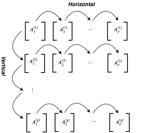
Figure 1: Reusing preconditioners in the AIRGA algorithm.

Next, we show how the new preconditioners are computed for both, the horizontal direction and the vertical direction. While looking at the horizontal route, let,

$A^{(z)}_{i-1}=\left(s_{i-1}^{(z)}\right)^{2}M+s_{i-1}^{(z)}D+K$ and

$A^{(z)}_{i}=\left(s_{i}^{(z)}\right)^{2}M+s_{i}^{(z)}D+K$ be the two coefficient matrices for different expansion points $s_{i-1}^{(z)}$ and $s_{i}^{(z)}$, respectively, with $i=2,\ \ldots,\ \ell$. Using the above theory, we enforce $A^{(z)}_{i-1}P^{(z)}_{i-1}=A^{(z)}_{i}P^{(z)}_{i}$ in Figure 2.

Figure 2: Expressing one linear system matrix in terms of the other.

Thus, we eventually enforce $A^{(z)}_{i-1}P^{(z)}_{i-1}=A^{(z)}_{i}Q^{(z)}_{i}P^{(z)}_{i-1}$ and solve the minimization problem

$$\min_{Q^{(z)}_{i}}\|A^{(z)}_{i-1}-A^{(z)}_{i}Q^{(z)}_{i}\|^{2}_{f}.$$

This gives us the new preconditioner $P^{(z)}_{i}=Q^{(z)}_{i}P^{(z)}_{i-1}$. This minimization is again performed for $n$ independent least square problems as in (7). Similar steps are followed for reusing preconditioners along the rest of the horizontal directions, i.e. for all $z=1,\ \ldots,\ \mathfrak{z}$.

Now, applying this technique for the vertical direction, we have $\text{for}\ z=2,\ \ldots,\ \mathfrak{z}$

$$A_{1}^{(z-1)}P_{1}^{(z-1)}=A_{1}^{(z)}P_{1}^{(z)}.$$

Following the steps as for the horizontal direction, here, we solve the minimization problem

$$\min_{Q^{(z)}_{1}}\|A^{(z-1)}_{1}-A^{(z)}_{1}Q^{(z)}_{1}\|^{2}_{f}.$$

This gives us the new preconditioner $P^{(z)}_{1}=Q^{(z)}_{1}P^{(z-1)}_{1}$. Again, this is solved as $n$ independent least square problems as in (7).

AIRGA with an efficient implementation of the above discussed theory of reusing preconditioners is given in Algorithm 1. If we closely look at line 4 of Algorithm 1, the solution vector is denoted by $X^{(0)}(s_{i})$, where the superscript $``0"$ refers to the index of the inner while loop (line 8). We do not bother about this index because, as earlier, matrix does not change inside this inner loop. Rather, we need to capture the change because of the outer while loop indexed with $z$. Hence, we denote the solution vector as $\mathcal{X}^{(z)}(s_{i})$ in Algorithm 1 (lines 8, 11, 19 & 22). It is important to emphasize again that preconditioners are never computed explicitly. Rather, they are obtained using matrix-vector product (please see line numbers 11, 19 & 22 of Algorithm 1).

Algorithm 1 : AIRGA with reuse of SPAI preconditioner

1:$z=1$

2:while no convergence do

3:     if $z==1$ then

4:         for $i=1,\ \ldots,\ \ell$ do

5:

6:              $A_{i}^{(1)}=\left(\left(s_{i}^{(1)}\right)^{2}M+\left(s_{i}^{(1)}\right)D+K\right)$

7:

8:              if $i==1$ then

9:                  Compute initial $P_{1}^{(1)}$ by solving

10:        $\min\limits_{P_{1}^{(1)}}\|I-A_{1}^{(1)}P_{1}^{(1)}\|_{f}^{2}$

11:      (First-time; no earlier preconditioner)

12:

13:                  $A_{1}^{(1)}P_{1}^{(1)}\mathcal{X}^{(1)}(s_{1})=F$

14:              else

15:                  Compute $Q_{i}^{(1)}$ by solving

16:        $\min\limits_{Q_{i}^{(1)}}\|A_{i-1}^{(1)}-A_{i}^{(1)}Q_{i}^{(1)}\|_{f}^{2}$

17:      (Reuse along horizontal direction)

18:

19:                  $A_{i}^{(1)}[{Q_{i}^{(1)}\ \cdots\ Q_{2}^{(1)}}P_{1}^{(1)}]\mathcal{X}^{(1)}(s_{i})=F$

20:              end if

21:         end for

22:     else

23:         for $i=1,\ \ldots,\ \ell$ do

24:

25:              $A_{i}^{(z)}=\left(\left(s_{i}^{(z)}\right)^{2}M+\left(s_{i}^{(z)}\right)D+K\right)$

26:

27:              if $i==1$ then

28:                  Compute $Q_{1}^{(z)}$ by solving

29:        $\min\limits_{Q_{1}^{(z)}}\|A_{1}^{(z-1)}-A_{1}^{(z)}Q_{1}^{(z)}\|_{f}^{2}$

30:      (Reuse along vertical direction)

31:

32:                  $A_{1}^{(z)}\left[Q_{1}^{(z)}\ \ldots\ Q_{1}^{(2)}\ P_{1}^{(1)}\right]\mathcal{X}^{(z)}(s_{1})=F$

33:              else

34:                  Compute $Q_{i}^{(z)}$ by solving

35:        $\min\limits_{Q_{i}^{(z)}}\|A_{i-1}^{(z)}-A_{i}^{(z)}Q_{i}^{(z)}\|_{f}^{2}$

36:      (Reuse along horizontal direction)

37:

38:                  $A_{i}^{(z)}\left[\underbrace{Q_{i}^{(z)}\ \cdots\ Q_{2}^{(z)}}\right.$

39:

40:        $\left.\underbrace{Q_{1}^{(z)}\ \ldots\ Q_{1}^{(2)}}\ P_{1}^{(1)}\right]\mathcal{X}^{(z)}(s_{i})=F$

41:              end if

42:         end for

43:     end if

44:     “All the given set of expansion points

45:  (i.e. $s_{1},\ s_{2},\ \ldots,\ s_{\ell}$) are updated”

46:     $z=z+1$

47:end while

48:Note: The minimization problems at lines 7, 10, 18 and 21 are solved as $n$ independent least square problems (see (7)).

For sake of brevity, reusing preconditioners in BIRKA (Algorithm 2) is discussed as part of Appendix A. Similarly, applying this theory to QB-IHOMM (Algorithm 3) is discussed in Appendix B.

IV Numerical Experiments

For supporting our proposed preconditioned iterative solver theory using the AIRGA algorithm [15], we perform experiments on two models. The first is a macroscopic equations of motion model (i.e. academic disk brake $M_{0}$) [38], and is discussed in Section IV-A. The second is also a similar model, however, this is a real-life industrial problem (i.e. industrial disk brake $M_{1}$) [38]. The experiments on this model are discussed in Section IV-B. These models are described by the following set of equations [38]:

$$\begin{split}M_{\Omega}\ddot{x}(t)=&-D_{\Omega}\dot{x}(t)-K_{\Omega}x(t)+Fu(t),\\ y(t)=&\ C^{T}x(t),\end{split}$$ (9)

where $M_{\Omega}=M,\ K_{\Omega}=K_{E}+K_{R}+\Omega^{2}K_{G},\ D_{\Omega}=\alpha M_{\Omega}+\beta K_{\Omega}$ (case of proportionally damped system; as needed for AIRGA) with commonly used parameter values as ${\Omega}=2\pi,\ \alpha=5\times 10^{-02},$ and $\beta=5\times 10^{-06}$. Further, $F\in\mathbb{R}^{n}\ \text{and}\ C^{T}\in\mathbb{R}^{n}$ are taken as $\left[1\ 0\ \cdots\ 0\right]^{T}$, which is the most frequently used choice. We take four expansion points linearly spaced between 1 and 500 based upon experience.

Although our purpose is to just reuse SPAI in AIRGA (Algorithm 1), we also execute original SPAI in AIRGA (Algorithm 1) for comparison. In Algorithms 1 and 1, at line 2 the overall iteration (while-loop) terminates when the change in the reduced model (computed as $H_{2}$-error between the reduced models at two consecutive AIRGA iterations) is less than a certain tolerance. We take this tolerance as $10^{-04}$ based upon the values in [15]. There is one more stopping criteria in Algorithms 1 at line 8 (also in Algorithm 1 but not listed here). This checks the $H_{2}$-error between two temporary reduced models. We take this tolerance as $10^{-06}$, again based upon the values in [15]. Since this is an adaptive algorithm, the optimal size of the reduced model is determined by the algorithm itself, and is denoted by $r$.

The linear systems that arise here have non-symmetric matrices. There are many iterative methods available for solving such linear systems. We use the Generalized Minimal Residual (GMRES) method [32] because it is very popular [40]. The stopping tolerance in GMRES is taken as $10^{-06}$, which is a common standard. As mentioned in Introduction, for both the given models, we observe that unpreconditioned GMRES fails to converge. Hence, we use the SPAI preconditioner as described above (without and with reuse). We use Modified Sparse Approximate Inverse (MSPAI 1.0) proposed in [39] as our preconditioner. This is because MSPAI uses a linear algebra library for solving sparse least square problems that arise here. We use standard initial settings of MSPAI $\left(\text{i.e. tolerance (ep) of}\ 10^{-04}\right)$.

We perform our numerical experiments on a machine with the following configuration: Intel Xeon (R) CPU E5-1620 V3 $@$ 3.50 GHz., frequency 1200 MHz., 8 CPU and 64 GB RAM. All the codes are written in MATLAB (2016b) (including AIRGA, GMRES) except SPAI and reusable SPAI. MATLAB is used because of ease of rapid prototyping. Computing SPAI and reusable SPAI in MATLAB is expensive, therefore, we use C++ version of these (SPAI is from MSPAI and reusable SPAI is written by us). MSPAI further uses BLAS, LAPACK and ATLAS libraries. Whenever a preconditioner has to be computed, we first compute SPAI and reusable SPAI separately (in-parallel) and save them. Then, we run MATLAB code along with the saved preconditioner matrices (i.e. SPAI and reusable SPAI).

IV-A Academic Disk Brake Model

This model is of size $4,669$. Based upon experience, the maximum reduced system size ($r_{max}$) is taken as $20$. As mentioned earlier, however, due to the adaptive nature of the AIRGA algorithm, we obtain a reduced system of size $r=13$. For this model, the AIRGA algorithm takes two outer iterations (line 2 of Algorithms 1 and 1) to converge (i.e. $\mathfrak{z}=2$).

Reusing the SPAI preconditioner is beneficial when the values of $\|I-A_{i}^{(z)}\|_{f}/\|I\|_{f}$ is large, and the values of $\|A_{i-1}^{(z)}-A_{i}^{(z)}\|_{f}/\|A_{i-1}^{(z)}\|_{f}$ and $\|A_{1}^{(z-1)}-A_{1}^{(z)}\|_{f}/\|A_{1}^{(z-1)}\|_{f}$ are small, which is true in this case (see Table III). In this table, columns 1 and 2 list the AIRGA iterations and the four expansion points, respectively. The above three quantities are listed in columns 3, 4 and 5, respectively. For the first AIRGA iteration and the first expansion point, SPAI preconditioner cannot be reused because there is no earlier preconditioner (mentioned as NA in table). From the second expansion point (and the first AIRGA iteration), we perform horizontal reuse of preconditioner (see Figure 1). This is the same for the second AIRGA iteration as well. Vertical reuse of preconditioner is done only for the first expansion point (and the second AIRGA iteration; again see Figure 1).

In Table IV, we compare the SPAI and the reusable SPAI timings. As for Table III, here columns 1 and 2 list the AIRGA iterations and the four expansion points, respectively. SPAI and reusable SPAI computation times are given in columns 3 and 4, respectively. At the first AIRGA iteration and the first expansion point, both SPAI and reusable SPAI take the same computation time. This is because, as above, reusing of SPAI preconditioner is not applicable here. From the second expansion point of the first AIRGA iteration, we see substantial savings because of the reuse of the SPAI preconditioner (approximately $68\%$).

TABLE III: SPAI and reusable SPAI analysis for the academic disk brake model.

AIRGA Itr.†	Exp. Pts.‡	SPAI Case	Reusable SPAI Case
1		Standard $\footnotesize{\dfrac{\|I-A_{i}^{(z)}\|_{f}}{\|I\|_{f}}}$	Horizontal $\footnotesize{\dfrac{\|A_{i-1}^{(z)}-A_{i}^{(z)}\|_{f}}{\|A_{i-1}^{(z)}\|_{f}}}$	Vertical $\footnotesize{\dfrac{\|A_{1}^{(z-1)}-A_{1}^{(z)}\|_{f}}{\|A_{1}^{(z-1)}\|_{f}}}$
	1	$3.77\times 10^{06}$	NA	NA
	2	$4.36\times 10^{06}$	$0.1569$
	3	$4.95\times 10^{06}$	$0.3139$	NA
	4	$5.54\times 10^{06}$	$0.4708$
2	1	$7.63\times 10^{06}$	NA	$0.9996$
	2	$4.06\times 10^{06}$	$0.0180$
	3	$1.62\times 10^{06}$	$20.3431$	NA
	4	$3.82\times 10^{06}$	$0.4985$

• AIRGA Iterations.

• Expansion Points.

TABLE IV: SPAI and reusable SPAI computation time for the academic disk brake model.

AIRGA Iterations $(z)$	Expansion Points $(s_{i})$	SPAI (Seconds)	Reusable SPAI (Seconds)
1	1	174	174
	2	164	10
	3	165	16
	4	165	20
2	1	165	64
	2	165	10
	3	165	108
	4	158	20
Total	8	1321	422

Table V provides the iteration count and the computation time of GMRES. Here, we only provide GMRES execution details since the computation time of preconditioner has been discussed above. In this table, column 1 lists the AIRGA iterations. The number of linear solves and average GMRES iterations per linear solve are given in columns 2 and 3, respectively. Finally, columns 4 and 5 list the computation times of GMRES when using SPAI and reusable SPAI, respectively. We notice from this table that solving linear systems by GMRES with SPAI takes less computation time as compared to solving them by GMRES with reusable SPAI. This is because when we reuse the SPAI preconditioner in GMRES, additional matrix-vector products are performed, however, this extra cost is almost negligible when compared to the savings in the preconditioner computation time for the latter case (as evident in Table III above; also see total GMRES and preconditioner time below).

Table VI gives the computation time of GMRES plus SPAI (column 2) and GMRES plus reusable SPAI (column 3) at each AIRGA iteration (column 1). As evident from this table, reusing the SPAI preconditioner leads to about $60\%$ savings in total time required for solving all the linear systems.

TABLE V: GMRES computation time for the academic disk brake model.

AIRGA Iterations $(z)$	No. of Linear Solves	GMRES Iterations per Linear Solve	GMRES Time when Using SPAI (Seconds)	GMRES Time when Using Reusable SPAI (Seconds)
1	10	271	$7.98$	$8.62$
2	13	270	$8.12$	$8.93$
[b]      Total	$\mathbf{23}$	${10\times 271+13\times 270}$ $\mathbf{=6220}$	${10\times 7.98+13\times 8.12}$ $\mathbf{=185}$	${10\times 8.62+13\times 8.93}$ $\mathbf{=202}$

TABLE VI: GMRES with SPAI and reusable SPAI computation time for the academic disk brake model.

AIRGA Iterations $(z)$	GMRES Plus SPAI Time (Seconds)	GMRES Plus Reusable SPAI Time (Seconds)
1	748	306
2	759	318
Total	1507	624

IV-B Industrial Disk Brake Model

This model is of size $1.2$ million. Based upon experience, the maximum reduced system size ($r_{max}$) is taken as $100$. As mentioned earlier, however, due to the adaptive nature of the AIRGA algorithm, we obtain a reduced system of size $r=52$. For this model, the AIRGA algorithm takes four outer iterations (line 2 of Algorithms 1 and 1) to converge (i.e. $\mathfrak{z}=4$).

Again, reusing the SPAI preconditioner is beneficial when the value of $\|I-A_{i}^{(z)}\|_{f}/\|I\|_{f}$ is large, and the value of $\|A_{i-1}^{(z)}-A_{i}^{(z)}\|_{f}/\|A_{i-1}^{(z)}\|_{f}$ and $\|A_{1}^{(z-1)}-A_{1}^{(z)}\|_{f}/\|A_{1}^{(z-1)}\|_{f}$ are small, which is true in this case (see Table VIII). The structure of this table is same as Table III. As earlier, for the first AIRGA iteration and the first expansion point, SPAI preconditioner cannot be reused because there is no earlier preconditioner (mentioned as NA in table). From the second expansion point (and the first AIRGA iteration), we perform horizontal reuse of preconditioner (see Figure 1). This is the same for the second, the third and the fourth AIRGA iterations as well. Vertical reuse of preconditioner is done only for the first expansion point (and the second, the third, and the fourth AIRGA iterations; again see Figure 1).

TABLE VII: SPAI and reusable SPAI analysis for the industrial disk brake model.

AIRGA Iterations $(z)$	Expansion Points $(s_{i})$	SPAI Case	Reusable SPAI Case
1		Standard $\footnotesize{\dfrac{\|I-A_{i}^{(z)}\|_{f}}{\|I\|_{f}}}$	Horizontal $\footnotesize{\dfrac{\|A_{i-1}^{(z)}-A_{i}^{(z)}\|_{f}}{\|A_{i-1}^{(z)}\|_{f}}}$	Vertical $\footnotesize{\dfrac{\|A_{1}^{(z-1)}-A_{1}^{(z)}\|_{f}}{\|A_{1}^{(z-1)}\|_{f}}}$
	1	$6.54\times 10^{08}$	NA	NA
	2	$6.54\times 10^{08}$	$3.74\times 10^{-05}$
	3	$6.54\times 10^{08}$	$7.49\times 10^{-05}$	NA
	4	$6.54\times 10^{08}$	$1.12\times 10^{-04}$
2	1	$1.31\times 10^{09}$	NA	$1.006$
	2	$6.65\times 10^{08}$	$0.49$
	3	$6.53\times 10^{08}$	$0.50$	NA
	4	$6.56\times 10^{08}$	$0.49$
3	1	$1.30\times 10^{09}$	NA	$1.009$
	2	$7.01\times 10^{08}$	$0.4658$
	3	$6.53\times 10^{08}$	$0.5499$	NA
	4	$6.63\times 10^{08}$	$0.4940$
4	1	$1.31\times 10^{09}$	NA	$1.0015$
	2	$6.86\times 10^{08}$	$0.4641$
	3	$6.53\times 10^{08}$	$0.5002$	NA
	4	$6.56\times 10^{08}$	$0.4933$

TABLE VIII: SPAI and reusable SPAI computation time for the industrial disk brake model.

AIRGA Iterations $(z)$	Expansion Points $(s_{i})$	SPAI$\S$	Reusing SPAI$\S$
1	1	10 hrs	10 hrs
	2	10 hrs	1 hr
	3	10 hrs	1 hr
	4	10 hrs	1 hr
2	1	10 hrs	1 hr 30 mins
	2	10 hrs	1 hr
	3	10 hrs	1 hr
	4	10 hrs	1 hr
3	1	10 hrs	1 hr 30 mins
	2	10 hrs	1 hour
	3	10 hrs	1 hour
	4	10 hrs	1 hour
4	1	10 hrs	1 hr 30 mins
	2	10 hrs	1 hr
	3	10 hrs	1 hr
	4	10 hrs	1 hr
Total	16	160 hrs	26 hrs 30 mins

• All times given here differ in seconds (not evident because of the rounding to the nearest minute).

In Table VIII, we compare the SPAI and the reusable SPAI timings. The structure of this table is same as that of Table IV. As before, at the first AIRGA iteration and the first expansion point, both SPAI and reusable SPAI take the same computation time. This is because, as above, reusing of SPAI preconditioner is not applicable here. From the second expansion point of the first AIRGA iteration, we see substantial savings because of the reuse of the SPAI preconditioner (from $160$ hours to $26$ hrs $30$ minutes; approximately $83\%$).

Table IX provides the iteration count and the computation time of GMRES. Here, again we have only provided GMRES execution details since the computation time of the preconditioner has already been discussed above. The structure of this table is same as that of Table V. As earlier, we notice from this table that solving linear systems by GMRES with SPAI takes less computation time as compared to solving them by GMRES with reusable SPAI. This is again because of additional matrix-vector products in the reusable SPAI case. Here also, this extra cost is almost negligible when compared to the savings in the preconditioner computation time (as evident in Table VIII; also see the total GMRES and preconditioner time below).

Table X gives the computation time of GMRES plus SPAI (column 2) and GMRES plus reusable SPAI (column 3) at each AIRGA iteration (column 1). As before, it is evident from this table, reusing the SPAI preconditioner leads to about $64\%$ savings in total time (from $197$ hours $28$ minutes to $72$ hours $06$ minutes).

TABLE IX: GMRES computation time for the industrial disk brake model.

AIRGA Iterations $(z)$	No. of Linear Solves	GMRES Iterations per Linear Solve	GMRES Time when Using SPAI (Minutes)	GMRES Time when Using Reusable SPAI (Minutes)
1	64	$421$	$08$	$10$
2	64	$426$	$09$	$11$
3	64	$429$	$10$	$12$
4	52	$432$	$10$	$12$
Total	244	$64\times(421+426+429)$ $+\ 52\times 432$ $\mathbf{=104,128}$	$64\times(08+09+10)$ $+\ 52\times 10$ $\mathbf{=2248}$	$64\times(10+11+12)$ $+\ 52\times 12$ $\mathbf{=2736}$

To demonstrate the quality of the reduced system, we plot the relative $H_{2}$ error between the transfer function of the original system and the reduced system with respect to the different expansion points (in Figure 3). The reduced system considered here is obtained by using GMRES with reusable SPAI. These expansion points, denoted by $S$, are computed as $2\pi f$, where the frequency variable $f$ is linearly spaced between $1$ and $500$. As evident from this figure, the obtained reduced system is good (the error is very small). Further, we also observe from this figure that the reduced model is most accurate in 7–10 range of the expansion points. This is because the final expansion points, upon the convergence of the AIRGA algorithm, lie in this range.

Figure 3: Relative error between the original and reduced system for the industrial disk brake model.

TABLE X: GMRES with SPAI and reusable SPAI computation time for the industrial disk brake model.

AIRGA Iterations $(z)$	GMRES plus SPAI Time	GMRES plus Reusable SPAI Time
1	$48\ \text{hrs}\ 32\ \text{mins}$	$23\ \text{hrs}\ 40\ \text{mins}$
2	$49\ \text{hrs}\ 36\ \text{mins}$	$16\ \text{hrs}\ 14\ \text{mins}$
3	$50\ \text{hrs}\ 40\ \text{mins}$	$17\ \text{hrs}\ 18\ \text{mins}$
4	$48\ \text{hrs}\ 40\ \text{mins}$	$14\ \text{hrs}\ 54\ \text{mins}$
Total	$\mathbf{197\ \text{\bf hrs}\ 28\ \text{\bf mins}}$	$\mathbf{72\ \text{\bf hrs}\ 06\ \text{\bf mins}}$

V Conclusions & Future Work

In this work, we have focused on MOR of non-parametric dynamical systems, specifically on the following three algorithms: AIRGA, BIRKA, and QB-IHOMM. Since solving large and sparse linear systems is a bottleneck in scaling these MOR algorithms for reduction of large sized dynamical systems, we have proposed reusing of the SPAI preconditioner.

Specifically, we have demonstrated the following: exploitation of the simplicity because of the lack of parameters in reusing preconditioners, multiple ways of reusing preconditioners within the algorithm, efficient implementation to ensure that the savings because of reusing preconditioners are not negated by bad coding, and experimentation on a massively large industrial problem. Numerical experiments show the effectiveness of our approach, where for a problem of size $1.2$ million, we save upto $64\%$ in the computation time. In absolute terms, this gives a saving of $5$ days.

In future, we plan to explore two directions. The first is use of the randomized preconditioners in solving linear systems arising in MOR. This is giving promising results. The second is to use the spiking neural networks to optimize the parameters inside the preconditioners.

Appendix A

In the Algorithm 2, we solve linear systems of equations at lines 4 and 5. We first apply our proposed theory of reusing preconditioners to line 4, which is given as

$$vec\left(V\right)=\left(-\Lambda\otimes I_{n}-I_{r}\otimes K-\sum\limits_{\mathsf{j}=1}^{m}\check{\check{N}}^{T}_{\mathsf{j}}\otimes N_{\mathsf{j}}\right)^{-1}$$

$$\left(\check{\check{F}}^{T}\otimes F\right)\ {vec(I_{m})}.$$

Here, $\Lambda$ is a diagonal matrix comprising of interpolation points, which is updated at the start of the while loop at line 2. Let $A_{z-1}=-\Lambda_{z-1}\otimes I_{n}-I_{r}\otimes K-\sum\limits_{\mathsf{j}=1}^{m}\check{\check{N}}^{T}_{\mathsf{j}}\otimes N_{\mathsf{j}}$ and $A_{z}=-\Lambda_{z}\otimes I_{n}-I_{r}\otimes K-\sum\limits_{\mathsf{j}=1}^{m}\check{\check{N}}^{T}_{\mathsf{j}}\otimes N_{\mathsf{j}}$ be the coefficient matrices corresponding to $\Lambda_{z-1}$ and $\Lambda_{z}$, respectively $\left(\text{for}\ z=1,\ \ldots,\ \mathfrak{z}\ (\text{until covergence})\right)$. Expressing $A_{z}$ in terms of $A_{z-1}$, we get

$$A_{z}=A_{z-1}\left(I_{nr}+A_{z-1}^{-1}(-\Lambda_{z}\otimes I_{n})+A_{z-1}^{-1}(\Lambda_{z-1}\otimes I_{n})\right),$$

where $I_{nr}\in\mathbb{R}^{n\cdot r\times n\cdot r}$ is the Identity matrix. Now, we enforce

$$A_{z-1}P_{z-1}=A_{z}P_{z}\ \ or$$ (10)

$$A_{z-1}P_{z-1}=\ A_{z-1}\left(I_{nr}+A_{z-1}^{-1}(-\Lambda_{z}\otimes I_{n})+A_{z-1}^{-1}(\Lambda_{z-1}\otimes I_{n})\right)\cdot$$

$$\left(I_{nr}+A_{z-1}^{-1}(-\Lambda_{z}\otimes I_{n})+A_{z-1}^{-1}(\Lambda_{z-1}\otimes I_{n})\right)^{-1}P_{z-1}$$

$$=\ A_{z}P_{z},$$

where $P_{z}=\left(I_{nr}+A_{z-1}^{-1}(-\Lambda_{z}\otimes I_{n})+A_{z-1}^{-1}(\Lambda_{z-1}\otimes I_{n})\right)^{-1}P_{z-1}$.

Let $Q_{z}=\left(I_{nr}+A_{z-1}^{-1}(-\Lambda_{z}\otimes I_{n})+A_{z-1}^{-1}(\Lambda_{z-1}\otimes I_{n})\right)^{-1}$, then instead of (10) we enforce $A_{z-1}P_{z-1}=A_{z}Q_{z}P_{z-1}$. The remaining derivation here is same as earlier (see Section III-C). We reuse preconditioners at line 5 similarly.

Appendix B

In the Algorithm 3, we solve linear systems of equations at line 4 and 10. Again, we first apply our proposed theory of reusing preconditioners to line 4, which is given as

$$X_{j}(\sigma_{i})=[(\sigma_{i}D-K)^{-1}D]^{j}(\sigma_{i}D-K)^{-1}F,\$$

$$\text{for}\ j=1,\ \ldots,\ P+Q\ \text{and}\ i=1,\ \ldots,\ \ell.$$

Let $A_{i-1}=\sigma_{i-1}D-K$ and $A_{i}=\sigma_{i}D-K$ be the two coefficient matrices for different interpolation points $\sigma_{i-1}$ and $\sigma_{i}$, respectively $\left(\text{for}\ i=1,\ \ldots,\ \ell\right)$. Expressing $A_{i}$ in terms of $A_{i-1}$, we get

$$A_{i}=A_{i-1}(I+(\sigma_{i}-\sigma_{i-1})A_{i-1}^{-1}D).$$

Now, we enforce

$$A_{i-1}P_{i-1}=A_{i}P_{i}\ \ or$$ (11)

$$\begin{split}A_{i-1}P_{i-1}=\ A_{i-1}(I+(\sigma_{i}-\sigma_{i-1})A_{i-1}^{-1}D)\ \cdot\\ (I+(\sigma_{i}-\sigma_{i-1})A_{i-1}^{-1}D)^{-1}P_{i-1}\\ =\ A_{i}P_{i},\end{split}$$

where $P_{i}=(I+(\sigma_{i}-\sigma_{i-1})A_{i-1}^{-1}D)^{-1}P_{i-1}$.

Let $Q_{i}=(I+(\sigma_{i}-\sigma_{i-1})A_{i-1}^{-1}D)^{-1}$, then instead of (11) we enforce $A_{i-1}P_{i-1}=A_{i}Q_{i}P_{i-1}$. Again, here also, the remaining derivation is same as earlier (see Section III-C). We reuse preconditioners at line 10 similarly.

Navneet Pratap Singh received his bachelor’s degree in Computer Science and Engineering from UPTU, Lucknow, India, and his master’s degrees in Modelling and Simulation from the Defence Institute of Advanced Technology, Pune, India. He is currently pursuing his Ph.D. degree with IIT Indore. His thesis focuses on Stable Linear Solves with Preconditioner Updates for Model Reduction. His research interests are at the intersection of Computer Science and Mathematics, especially Numerical Linear Algebra, Optimization, Dynamical Systems, and Machine Learning.

Kapil Ahuja (B.Tech.: IIT (BHU), India; M.S. and Ph.D.: Virginia Tech, USA; Postdoctoral Research Fellow: Max Planck Institute, Germany) has a varied background, including degrees in Computer Science, Mathematics, and Mechanical Engineering. He is currently an Associate Professor in Computer Science and Engineering at IIT Indore (India). In the past, he has been a visiting professor at TU Braunschweig (Germany), TU Dresden (Germany), and Sandia National Labs (USA). Dr. Ahuja is working on Mathematics of Data Science as well as Computational Science. Specifically, Artificial Intelligence, Machine Learning, Numerical Methods, and Optimisation.

References

- [1] O. Katsuhiko, Modern Control Engineering. Upper Saddle River, NJ, USA: Prentice Hall PTR, 2001.
- [2] M. Rewienski and J. White, “A trajectory piecewise-linear approach to model order reduction and fast simulation of nonlinear circuits and micromachined devices,” IEEE Trans. Comput.-Aided Des. Integr. Circuits Syst., vol. 22, no. 2, pp. 155–170, 2003.
- [3] A. C. Antoulas, “Approximation of Large-Scale Dynamical Systems: An Overview,” IFAC Proceedings, vol. 37, no. 11, pp. 19–28, 2004.
- [4] A. C. Antoulas, Approximation of Large-Scale Dynamical Systems. Philadelphia, PA, USA: SIAM, 2005.
- [5] J. E. S. Socolar, Nonlinear Dynamical Systems. Boston, MA, USA: In Complex Systems Science in Biomedicine, T. S. Deisboeck and J. Y. Kresh Eds., Springer, 2006, pp. 115–140.
- [6] B. N. Bond, “Parameterized model order reduction for nonlinear dynamical systems,” Master’s dissertation, Dept. Elect. Eng. and Comp. Sci., MIT, Cambridge, MA, USA, 2006.
- [7] E. J. Grimme, “Krylov projection methods for model reduction,” Ph.D. dissertation, Dept. Elect. Eng., Univ. Illinois at Urbana-Champaign, Urbana, IL, USA, 1997.
- [8] S. Gugercin, “Projection methods for model reduction of large-scale dynamical systems,” Ph.D. dissertation, Dept. Elect. and Comp. Eng., Rice Univ., Houston, TX, USA, 2003.
- [9] W. H. Schilders, H. A. Van der Vorst and J. Rommes, Model Order Reduction: Theory, Research Aspects and Applications, Berlin, Germany: Springer, vol. 13, 2008.
- [10] S. Gugercin, A. C. Antoulas and C. Beattie, “ model reduction for large-scale linear dynamical systems,” SIAM J. Matrix Anal. Appl., vol. 30, no. 2, pp. 609–638, 2008.
- [11] T. Breiten, “Interpolation methods for model reduction of large-scale dynamical systems,” Ph.D. dissertation, Dept. Math., Otto-von-Guericke-Universität Magdeburg, Germany, 2013.
- [12] S. A. Wyatt, “Issues in interpolatory model reduction: Inexact solves, second-order systems and DAEs,” Ph.D. dissertation, Dept. Math., Virginia Tech, Blacksburg, VA, USA, 2012.
- [13] Q. Zhi-Yong, J. Yao-Lin and Y. Jia-Wei, “Interpolatory model order reduction method for second order systems,” Asian J. Control, vol. 20, no. 1, pp. 312–322, 2018.
- [14] Z. Bai and Y. Su, “Dimension reduction of large-scale second-order dynamical systems via a second-order Arnoldi method,” SIAM J. Sci. Comput., vol. 26, pp. 1692–1709, 2005.
- [15] T. Bonin, H. Faßbender, A. Soppa, and M. Zaeh, “A fully adaptive rational global Arnoldi method for the model-order reduction of second-order MIMO systems with proportional damping,” Math. Comput. Simulat., vol. 122, pp. 1–19, 2016.
- [16] P. Benner and T. Breiten, “Interpolation-based -model reduction of bilinear control systems,” SIAM J. Matrix Anal. Appl., vol. 33, no. 3, pp. 859–885, 2012.
- [17] G. M. Flagg, “Interpolation methods for the model reduction of bilinear systems,” Ph.D. dissertation, Dept. Math., Virginia Tech, Blacksburg, VA, USA, 2012.
- [18] R. Choudhary and K. Ahuja, “Inexact linear solves in model reduction of bilinear dynamical systems,” IEEE Access, vol. 7, pp. 72297-72307, 2019.
- [19] M. M. A. Asif, M. I. Ahmad, P. Benner, L. Feng, and T. Stykel, “Implicit higher-order moment matching technique for model reduction of quadratic-bilinear systems,” 2019, arXiv:1911.05400. [Online]. Available: https://arxiv.org/abs/1911.05400.
- [20] U. Baur, C. Beattie, P. Benner and S. Gugercin, “Interpolatory projection methods for parameterized model reduction,” SIAM J. Sci. Comput., vol. 33, no. 5, pp. 2489–2518, 2011.
- [21] P. Benner and L. Feng, A Robust Algorithm for Parametric Model Order Reduction Based on Implicit Moment Matching: In Reduced Order Methods for Modeling and Computational Reduction, A. Quarteroni and G. Rozza, Eds., Springer, 2014, pp. 159–185.
- [22] L. Feng, P. Benner and J. G. Korvink, “Subspace recycling accelerates the parametric macro-modeling of MEMS,” Int. J. Numer. Meth. Engng., vol. 94, pp. 84–110, 2013.
- [23] A. C. Rodriguez, S. Gugercin, and J. Borggaard, “Interpolatory model reduction of parameterized bilinear dynamical systems,” Adv. Comput. Math., vol. 44, pp. 1887–1916, 2018.
- [24] X. Cao, “Optimal model order reduction for parametric nonlinear systems,” Ph.D. dissertation, Dept. Math. and Comp. Sci., TU Eindhoven, Netherlands, 2019.
- [25] K. Ahuja, E. de Sturler, S. Gugercin and E. R. Chang, “Recycling BiCG with an application to model reduction,” SIAM J. Sci. Comput., vol. 34, no. 4, pp. A1925–A1949, 2012.
- [26] K. Ahuja, P. Benner, E. de Sturler and L. Feng, “Recycling BiCGSTAB with an application to parametric model order reduction,” SIAM J. Sci. Comput., vol. 37, no. 5, pp. S429–S446, 2015.
- [27] K. Ahuja, “Recycling Krylov subspaces and preconditioners,” Ph.D. dissertation, Dept. Math., Virginia Tech, Blacksburg, VA, USA, 2011.
- [28] K. Ahuja, B. K. Clark, E. de Sturler, D. M. Ceperley and J. Kim, “Improved scaling for quantum Monte Carlo on insulators,” SIAM J. Sci. Comput., vol. 33, no. 4, pp. 1837–1859, 2011.
- [29] A. K. Grim-McNally, E. de Sturler and S. Gugercin, “Preconditioning parametrized linear systems,” 2017, arXiv:1601.05883v3. [Online]. Available: https://arxiv.org/abs/1601.05883.
- [30] A. K. Grim-McNally, “Reusing and updating preconditioners for sequences of matrices,” Master’s dissertation, Dept. Math., Virginia Tech, Blacksburg, VA, USA, 2015.
- [31] N. P. Singh, and K. Ahuja, “Preconditioned linear solves for parametric model order reduction,” Int. J. Comput. Math., 2019, 10.1080/00207160.2019.1627525.
- [32] Y. Saad, Iterative Methods for Sparse Linear Systems, Philadelphia, PA, USA: SIAM, 2003.
- [33] H.-L. Shen, S.-Y. Li, and X.-H. Shao, “The NMHSS iterative method for the standard Lyapunov equation,” IEEE Access, vol. 7, pp. 13200–13205, 2019.
- [34] M. Benzi, “Preconditioning techniques for large linear systems: A survey,” J. Comput. Phys., vol. 182, no. 2, pp. 418–477, 2002.
- [35] M. Grote and T. Huckle, “Parallel preconditioning with sparse approximate inverses,” SIAM J. Sci. Comput., vol. 18, no. 3, pp. 838–853, 1997.
- [36] E. Chow and Y. Saad, “Approximate inverse preconditioners via sparse-sparse iterations,” SIAM J. Sci. Comput., vol. 19, no. 3, pp. 995–1023, 1998.
- [37] M. Fallah and S. A. Edalatpanah, “On the some new preconditioned generalized AOR methods for solving weighted linear least squares problems,” IEEE Access, vol. 8, pp. 33196–33201, 2020.
- [38] N. Gräbner, V. Mehrmann, S. Quraishi, C. Schröder and V. U. Wagner, “Numerical methods for parametric model reduction in the simulation of disk brake squeal,” J. Appl. Math. Mech., vol. 96, no. 12, pp. 1388–1405, 2016.
- [39] K. Alexander, “Modified sparse approximate inverses (MSPAI) for parallel preconditioning,” Ph.D. dissertation, Dept. Math., TU Munich, Germany, 2008.
- [40] T. Han and Y. Han, “Numerical solution for super large scale systems,” IEEE Access, vol. 1, pp. 537–544, 2013.