The effect of photoionising feedback on the shaping of hierarchically-forming stellar clusters

Abstract

We use two hydrodynamical simulations (with and without photoionising feedback) of the self-consistent evolution of molecular clouds (MCs) undergoing global hierarchical collapse (GHC), to study the effect of the feedback on the structural and kinematic properties of the gas and the stellar clusters formed in the clouds. During this early stage, the evolution of the two simulations is very similar (implying that the feedback from low mass stars does not affect the cloud-scale evolution significantly) and the star-forming region accretes faster than it can convert gas to stars, causing the instantaneous measured star formation efficiency (SFE) to remain low even in the absence of significant feedback. Afterwards, the ionising feedback first destroys the filamentary supply to star-forming hubs and ultimately removes the gas from it, thus first reducing the star formation (SF) and finally halting it. The ionising feedback also affects the initial kinematics and spatial distribution of the forming stars, because the gas being dispersed continues to form stars, which inherit its motion. In the non-feedback simulation, the groups remain highly compact and do not mix, while in the run with feedback, the gas dispersal causes each group to expand, and the cluster expansion thus consists of the combined expansion of the groups. Most secondary star-forming sites around the main hub are also present in the non-feedback run, implying a primordial rather than triggered nature. We do find one example of a peripheral star-forming site that appears only in the feedback run, thus having a triggered origin. However, this appears to be the exception rather than the rule, although this may be an artifact of our simplified radiative transfer scheme.

1 Introduction

Stellar groups are the result of star formation (SF) happening within dense molecular gas. However, it remains a challenge to have a complete description for the origin and the structural properties of stellar clusters (SCs), such as mass segregation, density profiles, age gradients and histograms, hierarchical structure, etc.

From the observational point of view, great advances have been achieved in the study of kinematics of SCs with data from surveys like GAIA-DR2 (Kounkel et al., 2018) and APOGEE-2 (see e.g., Hacar et al., 2016; Da Rio et al., 2017; Kounkel et al., 2018). In particular, Da Rio et al. (2017) found evidence for kinematic subclustering and by studying the kinematic properties through radial velocities they found also some evidence for ongoing expansion; Hacar et al. (2016) have suggested that for most of the Orion A cloud, young stars keep memory of the parental gas substructure where they originated, and Kounkel et al. (2018) have identified distinct groups of stellar objects with ages ranging from 1 to 12 Myr within the Orion Complex. These authors also found subclusters and reported that, while in Orion D and $\lambda$ Ori the motions of the stars are consistent with an expansion process, Orion B is still in the process of contraction. Finally, Kounkel et al. (2018) also suggest that the proper motions in $\lambda$ Ori are consistent with a radial expansion due to a supernova explosion. These features require a coherent explanation within current models of formation of SCs and the MCs where they were formed. In particular, it is important to determine the role that stellar feedback from massive stars plays on this.

On the theory side, a variety of numerical models of star formation in the interstellar medium has been used to explain the properties of SCs following the complete evolution of molecular clouds since their own formation to the formation of a stellar group within the region. In particular, the effect of different sources of feedback and the positioning of the sources has been a matter of intense research. (see e.g., Bate, 2009; Vázquez-Semadeni, 2011; Colín et al., 2013; Dale et al., 2013; Dale et al., 2014; Iffrig & Hennebelle, 2015, 2017; Körtgen et al., 2016; Vázquez-Semadeni et al., 2017; Colling et al., 2018; Haid et al., 2018; Grudić et al., 2018a; Zamora-Avilés et al., 2019b). In particular, Haid et al. (2018) showed that the relative impact of stellar winds and ionising radiation depends on the stellar mass considered but even more strongly on the properties of the ambient medium. They found that for stars placed in the CNM, ionising radiation is the relevant source of feedback to take into account.

One important aspect, which perhaps has not received sufficient attention, is the need to investigate clouds in which both the geometry of the clouds and the positioning of the ionising feedback sources arise self-consistently, in order to avoid unrealistic setups. Numerical simulations of the formation and evolution of the clouds in the presence of self-gravity indicate that the clouds engage in global hierarchical collapse (GHC; Vázquez-Semadeni et al., 2019, and references therein), forming filamentary accretion flows that transfer mass from the large to the small scales (e.g., Heitsch et al., 2008, 2009; Smith et al., 2009; Gómez & Vázquez-Semadeni, 2014). For example, clouds formed self-consistently by collision of diffuse gas streams tend to be flattened and porous, with warm, diffuse gas “pockets”, rather than roundish and isothermal, and to develop turbulence due to the combined effect of various instabilities (e.g., Walder & Folini, 1998; Ballesteros-Paredes et al., 1999a; Hennebelle & Pérault, 2000; Hennebelle et al., 2008; Audit & Hennebelle, 2005; Heitsch et al., 2005, 2006; Vázquez-Semadeni et al., 2006). A realistic shape and porous constitution may be essential for the correct simulation and dispersal of the clouds, as discussed by Colín et al. (2013), Dale (2015), and Rey-Raposo et al. (2015).

In this paper we study structural properties of stellar clusters and the gas around them using hydrodynamical simulations in which the clouds have formed and evolved self-consistently from the collision of oppositely-directed streams of diffuse warm gas, with an additional moderate turbulent component to break the symmetry of the stream collision setup. The clouds then follow an evolutionary path consisting of growth, onset of global hierarchical collapse (GHC), accelerating star formation, cluster formation and cloud dispersal, as described in Vázquez-Semadeni et al. (2019).

In these simulations, we test the role of stellar feedback in shaping the properties of resulting stellar clusters and the gas that led to its formation and evolution. For this, we use hydrodynamical simulations presented first in Colín et al. (2013, hereafter Paper I) and then studied in the context of cluster formation in Vázquez-Semadeni et al. (2017, hereafter Paper II). We use the LAF1 simulation described in Paper I (for “large-amplitude fluctuations, feedback on”), focusing, in particular, on the cluster labeled G1-2 in Paper II. In the present paper, we investigate the effects of feedback in detail, by including the non- feedback counterpart of the LAF1 simulation, denoted LAF0. Besides pinpointing the precise effect of the feedback on the cluster structure, our results can additionally help to test the GHC scenario of MCs by testing its ability to form realistic clusters, and predict their observed properties.

This article is organized as follows. In Sec. 2.1 we present our simulations and describe the main physical processes included in the numerical code, and in Sec. 2.2 we discuss the procedure to analyze cluster properties. Next, in Sec. 3 we present our main results, which include an analysis of the feedback effect on gas, stars, and the SFR in the SC. In Sec. 4 we discuss the implications of our results and their comparison with other studies. Finally, in Sec. 5 we summarize our findings and present our conclusions.

2 Numerical setup and method

In this section we first describe the numerical simulations, albeit only briefly, as they have been already described in detail in Paper I and Paper II, to which we refer the reader for further details. We then describe the cluster-identification algorithm.

2.1 Simulations

We use the Hydrodynamics+N–body Adaptive Refinement Tree (ART) code (Kravtsov, Klypin & Khokhlov, 1997; Kravtsov, 2003) to run the simulations. The initial conditions consist of two oppositely directed cylindrical streams that collide within a 256 pc numerical box containing a total mass of $9.25\times 10^{5}$ $M_{\odot}$. The gas properties of the uniform background resemble the conditions of the warm neutral medium (WNM): it has a uniform density $n=1\ {\rm cm}^{-3}$ and temperature $T=5000$ K. The streams, which have the same density as the background, have a length of 112 pc, a radius of 32 pc, and travel at a speed of 5.9 ${\rm km~{}s}^{-1}$ each. This velocity is subsonic (Mach number of 0.8) with respect to the adiabatic sound speed of the WNM. The head-on collision of the streams promotes a transition to the cold phase, forming an initially circular sheet of cold, dense gas (cold neutral medium), whose thickness and mass grow as the warm gas from the streams accretes onto the layer and condenses to the cold phase (Vázquez-Semadeni et al., 2006). A turbulent initial velocity field with rms velocity dispersion of 1.7 ${\rm km~{}s}^{-1}$ is added in order to break the symmetry of the colliding streams and trigger various instabilities within the layer (Heitsch et al., 2006), which cause it to bend and fragment. This setup is meant to represent the formation of a large cloud by general transonic or supersonic compressions in the WNM of either turbulent or gravitational origin (e.g., von Weizsäcker, 1951; Roberts, 1969; Sasao, 1973; Elmegreen & Lada, 1977; Vishniac, 1994; Ballesteros-Paredes et al., 1999b; Hennebelle & Pérault, 2000; Koyama & Inutsuka, 2002; Audit & Hennebelle, 2005; Heitsch et al., 2005, 2006; Vázquez-Semadeni et al., 2006, 2007).

As the simulation evolves, and once the mass is redistributed forming cold dense regions, the simulation allows up to five refinement levels, reaching a minimum cell size of 0.0625 pc ($\approx$13 000 au). Cells in the mesh are refined when the gas mass within the cell is greater than 0.32 $M_{\odot}$. It is important to note that the cell’s mass can reach much larger values than this ‘refining mass’ after the maximum refining level is reached due to our probabilistic SF scheme (see 2.1.1 below).

As described in Paper I, we modified our original version of ART such that our simulations include: i) a new probabilistic SF prescription; ii) self-gravity from gas and stars; iii) parametrized heating and cooling, and iv) an ionisation feedback prescription by massive stars. We use the cooling and heating functions provided in Koyama & Inutsuka (2002),

$$\frac{\Lambda(T)}{\Gamma} =10^{7}\exp\left(\frac{-1.184\times 10^{5}}{T+1000}\right)$$

$$\;\;\;\;+1.4\times 10^{-2}\sqrt{T}\exp\left(\frac{-92}{T}\right)\rm{cm}^{3}$$ (1)

$$\Gamma=2.0\times 10^{-26}\rm{ergs}^{-1}.$$ (2)

This particular parametrization differs from the one presented in Koyama & Inutsuka (2002) since we have included the corrections to the typographical errors that appeared in the original version, as discussed in Vázquez-Semadeni et al. (2007). Under the conditions imposed by these functions the gas is thermally unstable in the density range 1 $\lesssim n\lesssim$ 10 $\rm{cm}^{3}$.

2.1.1 Star formation: a probabilistic approach

For each timestep of the coarsest grid, when the gas density $n$ in a grid cell exceeds a density threshold $n_{\rm SF}$, a stellar particle (SP) with mass $m_{\it SP}$ may be placed in the cell with a probability $P$. Indeed, depending on the value of $P$, there is a non-zero probability (1-$P$) of not forming an SP, even when the density cell reaches $n_{\rm SF}$. If this is the case, then the gas accretion into the cell continues for several timesteps until a SP is created. When an SP finally forms, it acquires half the gas mass of its parent cell, and does not accrete further. Thus, a cell that exceeds the density threshold but does not form a star can increase its density and mass until it eventually does form a star. This mimics the process of accretion onto a protostar to form a massive star. Indeed, the prescription we use implies that the longer it takes to form an SP in a collapsing cell, the more massive the SP will be, because the density of the cell will be higher.

Consequently, our probabilistic prescription allows the formation of SPs with different masses. In Paper I it was shown that the resulting mass distribution of the SPs is a power law with an exponent than can be tuned depending on the value of $P$. In particular, it was found in Paper I that, for $P=0.003$, the slope of the SP mass distribution (the simulation’s IMF) in run LAF1 simulation went from $-1.21$ at $\approx$ 6 Myr after the SF starts, to $-1.34$ at the end of the evolution, $\approx$ 21 Myr after the first star was formed, thus resembling the Salpeter IMF. Also, for our fiducial setup, with five refinement levels, $P=0.003$, and $n_{\rm SF}$$=9.2\times 10^{4}\;{\rm cm}^{-3}$, the minimum SP mass in the simulation was $m_{\rm SP}=0.39$ $M_{\odot}$, while the most massive has $m_{\rm SP}=61$ $M_{\odot}$ by the end of the simulation.

We also use the non-feedback counterpart of LAF1 simulation, labeled LAF0 in Paper I, as a ‘control simulation’ to test feedback effects. In this simulation, the most massive SP has $m_{\rm SP}\approx 100$ $M_{\odot}$ at its final time. As the SPs in our simulations have stellar masses, hereafter we will refer to them simply as ‘stars’.

2.1.2 Feedback scheme

For simplicity and cleanliness, in our simulation with feedback, we only consider a sub-grid model of UV photoionising radiation from massive stars. This choice is partially justified by the fact that a number of studies have concluded that this form of feedback is likely to be the dominant form of energy injection into giant molecular clouds (GMCs) leading to their dispersal (e.g., Matzner, 2002; Haid et al., 2019). Nevertheless, in a future work we plan to test other feedback sources.

For computing the ionising feedback from massive stars, in this work we first determine the size of an Hii region around the massive stars. To do that, we compute the Strömgren (1939) radius corresponding to the star’s mass as

$$R_{S}\equiv\left(\frac{3}{4\pi}\frac{S(M_{\star})}{\alpha n^{2}_{\rm LOS}}\right)^{1/3},$$ (3)

with $S(M_{\star})$ the ionising flux produced by a star of mass $M_{\star}$, $\alpha=3.0\times 10^{-13}{\rm cm}^{3}{\rm s}^{-1}$ the hydrogen recombination coefficient and $n_{\rm LOS}$ a uniform line-of-sight (LOS) characteristic density in the Hii region computed as the geometric mean of the density at the site of the star, $n_{\rm SP}$, and the density at the test grid cell, $n_{\rm tc}$, so that $n_{\rm LOS}=\sqrt{n_{\rm SP}n_{\rm tc}}$. In Paper I it was shown that this simplified prescription reproduces correctly the expansion of an Hii region, although it neglects the effect of “shadows” behind clumps. Nevertheless, our results are consistent, for example in measured global star formation efficiencies, with those obtained from simulations with full radiative transfer implemented (e.g., Zamora-Avilés et al., 2019a). For $S(M_{\star})$ we use tabulated data provided by Diaz-Miller, Franco & Shore (1998). We assume that only stars with masses greater than 1.9 $M_{\odot}$ inject any significant feedback into the ISM.

Once $R_{S}$ is computed for each line of sight, we assign a temperature of $10^{4}$ K to all cells whose distances $d_{\rm LOS}$ to the star satisfy $d_{\rm LOS}<R_{\rm S,LOS}$, and we turn off the cooling in these cells to prevent very dense cells from radiating their thermal energy too quickly. This thermal state will last for a time $t_{s}$ which depends on the mass of the star according to:

$$t_{s}=\left\{\begin{array}[]{lr}2\;{\rm Myr}&\text{if }m_{*}\leq 8{\rm M}_{\odot}\\ 222\;{\rm Myr}\left(\frac{m_{*}}{{\rm M}_{\odot}}\right)^{-0.95}&\text{if }m_{*}>8{\rm M}_{\odot}\end{array}\right.$$ (4)

For stars with $m_{*}$ lower than 8 $M_{\odot}$, this time characterizes their stellar wind phase, while for stars with $m_{*}$ greater than 8 $M_{\odot}$, $t_{s}$ is a fit to their lifetimes as given by Bressan et al. (1993). Note that with this feedback prescription we are accounting for non-local radiation effects: ionising photons from massive stars affect not only the parent cell where a star was born, but all the nearby cells within $R_{S}$. However, our single-fluid prescription does not follow the neutral and ionised components. As we mentioned above, we simply set the temperature of cells that are within the $R_{\rm S,LOS}$ from an ionising star to $10^{4}$ K, and then let them return to their thermal-equilibrium ($\Gamma=n\Lambda$) temperature once the star “turns off” according to the stellar lifetime given by eq. (4).

2.2 Procedure

A number of SCs were formed in the simulated box (see Paper II for its general description). In this work we select the G1–2 group to show the effect of the feedback on the gas distribution and on the stars around the SC. For simplicity, henceforth we will refer to G1–2 group as G2. This was born in a region clearly detached from other star forming regions (several tens of parsecs away) and allows us to start the analysis with an unambiguous membership identification of the stars. Note that other regions in the simulation start forming stars at almost the same time ($\pm$ 1 Myr) than G2; thus, ionising radiation from their massive stars does not affect the evolution of G2. Within this region there are approximately 390 $M_{\odot}$ in stars in the LAF1 simulation by the end of the last analysed snapshot, while in the LAF0 run, around 883 $M_{\odot}$ were converted into stars. Another filamentary-like star forming region which appeared in the LAF1 simulation will be the subject of a future analysis.

We will use the center of mass of the stellar cluster, denoted ${\rm CM}_{\rm s}$, as the origin of the reference frame to compute its properties. As the stars are the source of photoionisation feedback, the center of mass of the stellar distribution represents the natural framework to compute its effect on the surrounding gas distribution. In Paper I we made an effort to determine, at each snapshot in the simulation, the membership of stars to the G2 cluster disregarding runaway stars to update ${\rm CM}_{\rm s}$ in subsequent time steps. Instead, for simplicity, here we include in our analysis all the stars that were born clearly within the star forming region first identified at $t\approx 19$ Myr in the LAF1 simulation, and follow their evolution over $\approx$ 10 Myr. During this period, a number of small sub-units appear in the surroundings of G2. We easily identify these subgroups by eye, and we follow their evolution by tracking the positions of their stars.

Similarly to what is done for G2, the center of mass is also computed for each subgroup, and all the stars born within the radius determined by the outermost star are considered as a new stars belonging to the corresponding subgroup. Obviously, some complications arise when groups start to merge. When that is the case, the center of mass is now computed considering all the stars from the merged groups. We will discuss this with more detail in Sec. 3.4.

Given the center of mass of the stellar distribution, we compute several properties of the gas and stars within different radii to analyze the imprint of stellar feedback on them. Thus, we are not constraining our analysis to a particular region, such as the region within the radius of the group, since we do not attempt to define such radius. Obviously, the center of mass depends on the stars considered but, given our approach to measure the cluster properties at different radius, and the fact that the differences on the location of the center of mass when we exclude runaway stars are minimal, we do not expect that avoiding the definition of a radius group shall affect our results.

3 Results

3.1 General evolution of the simulation

In this section we provide a brief description of the evolution of the simulation that leads to the formation of the clusters studied. For further details, the reader is referred to Colín et al. (2013) and Vázquez-Semadeni et al. (2017).

The colliding streams form a cold dense layer through a shock and a condensation front (Koyama & Inutsuka, 2000; Vázquez-Semadeni et al., 2006). The layer becomes turbulent by a combination of various instabilities (Vishniac, 1994; Koyama & Inutsuka, 2002, 2004; Audit & Hennebelle, 2005; Heitsch et al., 2006; Inoue et al., 2006), with the turbulence being moderately supersonic with respect to the cold gas. However, due to the added turbuelent velocity field in the initial conditions, the layer is strongly bent. Furthermore, as noted in Sec. 2, the streams have a length of 112 pc, and collide in the central $(y,z)$ plane of the simulation. That is, the streams have a finite length, and are completely contained within the 256-pc numerical box. At their inwards speed of 5.9 ${\rm km~{}s}^{-1}$, they complete their collision after 18.7 Myr.

During this time, the layer has been increasing its thickness and column density at roughly constant mean volume density, until it exceeds its Jeans mass and begins to contract gravitationally. Due to the turbulent motions, however, the contraction is highly non-homologous and anisotropic, forming filaments that accrete from the cloud and funnel the gas to the collapse centers, in a river-like flow (Gómez & Vázquez-Semadeni, 2014; Vázquez-Semadeni et al., 2019). Moreover, when the filaments have increased their linear mass density sufficiently, they undergo local low-mass collapse that constitute secondary star-formation sites (Gómez & Vázquez-Semadeni, 2014) in the periphery of the main collapse centers, usually referred to as “hubs”, in a “conveyor-belt”-like fashion (Longmore et al., 2014).

Within this context, the first stars appear in the simulation at an absolute time (i.e., from the start of the simulation) $\sim 19$ Myr. In what follows, we analyse the properties of two stellar clusters that begin forming at this time. For simplicity, we describe the evolution in terms of the time measured after the onset of star formation ($t_{\rm SF}$) in this region, which we refer to as $t_{\rm age}=t-t_{\rm SF}$.

3.2 Indirect effect of the feedback on the stars via the gas

In Fig. 1 we show the spatial stellar distribution of the simulated cluster G2 in the runs without (LAF0, left panels) and with feedback (LAF1, right panels) at four different times (from top to bottom, $t=22.5,25.0,27.5$ and $29.1$ Myr since the start of the simulations). These correspond to times $t_{\rm age}\approx 3.7,6.2,8.7$ and $10.2$ Myr since the formation of the first star in the group. The gas density is color coded in the figure according to the color bar in each panel.

Fig. 1 directly illustrates one of our main results: once massive stars are born, feedback becomes dominant and not only sweeps the gas out of the stellar cluster $\sim 5$ Myr after the formation of its first star (see the right panel in the second line in Fig. 1 where an Hiilike region can be identified), but it also strongly affects the spatial distribution of the stars, which is much more extended by the final time in the run with feedback (see the right panel at the bottom in Fig. 1) than in the run without feedback. In the latter, the cluster is tightly concentrated within a region of $\approx 2$ pc of radius, with only a few smaller subunits appearing in the surroundings, which are clearly detached from the main cluster. Thus, feedback not only disperses the gas, but induces a more scattered initial configuration of the cluster which is not only due to the reduction in the gravitational potential of the region once the gas is removed. In addition, the gas being pushed away from the main hub continues to form stars for some time, and therefore those stars form at more distant locations from the CM than in the case without feedback. For example, in Fig. 1, the circles indicate the position of a clump/stellar group that in the run without feedback (left panels) undergoes a close encounter with the stellar group in the main hub, orbiting around it and producing a tidal tail of stars. The same clump in the run with feedback is pushed sideways by the expanding shell around the main hub, and thus never undergoes the close encounter with the hub and its stars.

The effect of the feedback is also manifest in that, in the non-feedback run LAF0, after 10 Myr of evolution since the formation of the first star (bottom left panel), the accretion along the filament onto the main hub continues, with the filament being as dense and well defined as at the start. Instead, in run LAF1, the dense gas has been almost completely evacuated in the neighbourhood of the cluster, with only traces of gas being left at the sites of secondary cores/groups.

Finally, the well-known effect of the stellar cluster expanding as the gas is removed due to the loss of the latter’s gravitational potential (e.g., Tutukov, 1978; Lada et al., 1984; Baumgardt & Kroupa, 2007; Parmentier et al., 2008) is also clearly seen in Fig. 1, which shows that the stellar distribution in the run with feedback is much more extended than that in the run with no feedback. In this case, the stellar expansion begins to be clearly noticeable $\sim 8$ Myr after the formation of the first star.

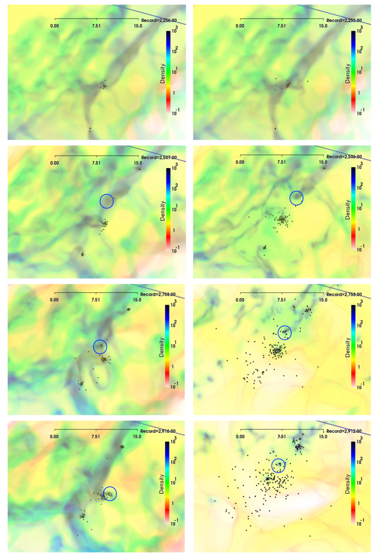
Figure 1: Non-Feedback (left panels) vs Feedback run (right panels) comparison of the G2 cluster in the simulated box at times $t=22.5,25.0,27.5$ and $29.1$ Myr since the start of the simulations. These times correspond to $t_{\rm age}\approx 3.7,6.2,8.7$ and $10.2$ Myr since the formation of the first star in the group. The color bar indicates the gas number density in ${\rm cm}^{-3}$. Note that the lower-density gas has a higher transparency in the rendering, and thus it is not very prominent. The ruler indicates a scale of 15 pc. Black dots represent individual stars born within the densest gas clumps. Ionising feedback from massive stars sweeps the gas out of the star forming region showing ring-shaped features in the gas distribution $\approx 5$ Myr after the formation of the stellar group (second panel from top at the right) and clear the region from gas after $\approx 10$ Myr (bottom panel at the right). Ionising feedback has a strong effect too in the spatial stellar distribution: the simulation including feedback forms more extended stellar clusters than the one without feedback. The circles indicate the position of a clump/stellar group that in the run without feedback (left panels) undergoes a close encounter with the stellar group in the main hub, but is pushed sideways by the expanding shell around the main hub in the run with feedback and thus avoids the close encounter.

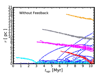
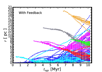
Figure 2: Stellar particle distribution as a function of $t_{\rm age}$, the elapsed time since the start of the formation of the cluster, for the run without feedback (LAF0, left panel) and the run with feedback (LAF1, right panel). The dots represent individual stars, and are colored according to their membership to the various subgroups, subG1 (cyan dots), subG2 (magenta dots), subG3 (grey dots), subG4 (orang dots), subG5 (red dots) and subG6 (green dots, only in the right panel). The stellar groups formed in run LAF0 are extremely concentrated (left panel), so some of them never merge with the others, while all groups merge in run LAF1, indicating that feedback promotes the mixing of the stellar populations by affecting their kinematic properties (right panel). Note also that one subgroup (green dots) forms at late times in run LAF1 that does not have a counterpart in run LAF0, constituting one (somewhat exceptional) instance of feedback-triggered star formation.

3.3 Masses of the most massive stars

The truncation of the gas supply along the filaments in the feedback run, LAF1, has the additional consequence of limiting the masses of the most massive stars that form. Specifically, the most massive star formed in the whole numerical box of run LAF1 has 61 $M_{\odot}$, while in run LAF0 it reaches 100 $M_{\odot}$. If we consider only the star forming region around G2, the most massive star in LAF1, formed $\approx 5$ Myr after SF began, has $\sim 30$ $M_{\odot}$, while the most massive star in run LAF0 has $\approx 60$ $M_{\odot}$, and forms around 8 Myr after the onset of SF. A stellar particle with a mass similar to that of the most massive star in LAF1 is formed more than a Myr before in run LAF0. Thus, feedback delays even more the formation of massive stars by controlling the accretion onto the star-forming hubs and clumps.

3.4 Hierarchical cluster assembly

The formation of smaller subunits or subgroups occurs in both runs, but as feedback “inflates” the stellar distribution, the subunits merge more rapidly in run LAF1, while they remain more clearly separate in run LAF0. Nevertheless, traces of their separate origins are still seen as local density enhancements in the resulting cluster. Also, it is important to note that the different secondary sites begin forming stars at different times. This is shown in Fig. 2, where we plot the 3D radial distance $r$ of each star (colored points) with respect to the centre of mass of the G2 cluster (points in blue) as a function of the time elapsed since the formation of the first star, $t_{\rm age}$. Only stars that were born within the G2 cluster at each time were used to compute the centre of mass. Thus, we explicitly exclude stars that form in a clearly different gas clump, even if they eventually merge with the G2 population.

As is shown in the right panel of Fig. 2, six subgroups form in the simulations that end up comprising group G2. We will refer to them as subG1 (cyan dots), subG2 (magenta dots), subG3 (grey dots), subG4 (orang dots), subG5 (red dots) and subG6 (green dots). In run LAF1, subgroups subg1 and subG5 fall onto G2 some time after their formation, while subgroups subG2, subG3 and subG6 are close enough to G2, that at late times, stars formed within these subgroups mix with the G2 population, without properly “falling” onto it. And viceversa, some stars from the central hub have been ejected, so at late times they have reached the locations of these subgroups. Subg4 is the outermost subgroup formed in this region of the numerical box, appearing $\sim 20$ pc away from the centre of mass of G2. Thus, we define the star forming region around G2 (SFRegG2) as the one that encloses all these subgroups; basically a 20-pc sphere around G2. This is somewhat arbitrary, but we will use it just to characterize the outskirts of G2, and our results do not depend sensitively on this choice. SFRegG2 manages to gather a mass $\la 10^{4}$$M_{\odot}$ in dense gas during its evolution; thus, our results should be compared to observational or numerical inferences obtained for MCs in this mass range.

Most of the subgroups form in small (“secondary”) collapsing sites within the filaments of dense gas that feed the main cluster G2. They started as small groups of stars confined to a small area, but a few megayears later they are dispersed due to the effect of feedback, either local, or from the main hub. SubG2 is the extreme case of this situation: as soon as feedback disperses the gas around G2, it also affects the stars constituting subG2, practically destroying it within a few megayears. Thus, in general, feedback from massive stars causes an expansion of the stars and, as a result, it facilitates the mixing of populations from different subgroups. Thus, possible “primordial” age gradients (Vázquez-Semadeni et al., 2017) might be blurred by this process. It is easy to verify that feedback from massive stars is the cause of this effect by comparing the left panel (run without feedback) with the right one (fiducial run including feedback) of Fig. 2: the subgroups form in both simulations, but are more tightly concentrated in run LAF0 in comparison to run LAF1. Thus, their populations never mix in LAF0, contrary to what occurs in LAF1 (compare the radial extents of each group in the two panels of Fig. 2).

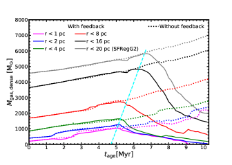
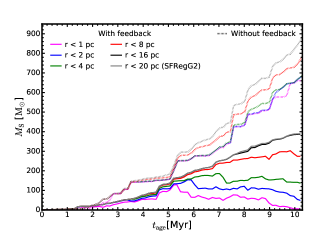
Figure 3: Left: Evolution of the dense gas mass enclosed within radii $r=1,2,4,8,16,20$ pc from the center of mass of G2. The solid and dotted lines respectively show the results for the simulations with (LAF1) and without (LAF0) feedback. The effect of feedback from massive stars in the dense gas mass distribution is clear at $\approx 5$ Myr after the formation of the first star ($t=0$ in this figure). The cyan dashed line in the left panel represents the times at which an expanding front moving at a speed of 11 ${\rm km~{}s}^{-1}$ intersects the various lines. Right: Evolution of the stellar mass in the same spherical regions as in the left panel. The stellar mass is seen to stop increasing or even decrease in the run with feedback, while it continues to increase at an accelerated pace in the run without feedback.

3.5 Dense gas consumption or removal?

The evolution of the SCs discussed above depends fundamentally on the amount of dense gas available to form stars at a given time. This reservoir depends on the accretion rate into the region, consumption to form stars (quantified by the SFR) and dispersal or evaporation due to feedback. In this work, we do not distinguish between dispersal and evaporation, and instead consider them together, referring to them generically as gas removal.

In order to determine how much gas is available to form stars as a function of time, the left panel of Fig. 3 shows the amount of dense gas (${n_{\rm dens}}>100\ {\rm cm}^{-3}$) enclosed within spheres of radius $r=1,2,4,8,16,$ and 20 pc from the center of mass of G2 for the two simulations. For comparison, the right panel of this figure shows the mass in stars within the same spherical regions.

As shown by the solid curves in the left panel of Fig. 3 (which denote the feedback run, LAF1), at time $t_{\rm age}\sim 5$ Myr, when the first very massive ($M=30$ $M_{\odot}$) star forms, an important qualitative change in the behaviour of the feedback simulation occurs: before that time, the mass in dense gas had been consistently increasing throughout region SFRegG2. However, after that time, the dense gas mass begins to decrease until there is no more dense gas in the innermost parts of SFregG2 at $t_{\rm age}\approx 10$ Myr. Thus, the gas is either fully consumed by star formation or fully removed by feedback within a radius of $\sim 4$ pc over a span of another $\sim 5$ Myr. On the other hand, in the non-feedback run LAF0, the dense gas mass simply continues to increase within all of the radii considered.

Note that the onset of the decrease of the dense gas mass occurs at later times for spheres of larger radii (see, for example, the curves for $r=16$ and 20 pc—black and grey curves, respectively—in Fig. 3). This is indicative of the expansion of the Hii region around the main hub, and implies a velocity $\approx 11$ ${\rm km~{}s}^{-1}$. It is important to note that the massive stars responsible for the ionising flux in the region were born just before the dense gas mass begins to decrease in the central parsec. That is, there is a time during which the star-forming region can accrete and grow essentially unimpeded, before the massive stars form. After this, the region is dispersed essentially in the crossing time of the sound speed in the ionised gas.

We define the dense gas mass removal rate from sphere of radius $r$ as

$$\dot{M}_{\rm g,dense} =-\frac{\Delta M_{\rm g,dense}(r)}{\Delta t}+\frac{\Delta M_{*}(r)}{\Delta t}$$ (5)

$$\equiv-\frac{\Delta M_{\rm g,dense}(r)}{\Delta t}+{\rm SFR(r),}$$

where the masses are computed inside radius $r$, $\Delta t$ is the elapsed time between two consecutive snapshots in the simulation ($\sim 0.14$ Myr), $M_{*}(r)$ is the mass in stars within radius $r$, the changes in the masses are computed over the time interval $\Delta t$, and the second equality defines the star formation rate within radius $r$, SFR$(r)$. By including the instantaneous SFR in the balance to compute $\dot{M}_{\rm g,dense}$ we account for gas consumption by conversion to stars. This also avoids spurious contributions by previously existing stars that enter or leave the spherical region.

As defined by Eq. (5), negative values of $\dot{M}_{\rm g,dense}$ imply that accretion is more important than dispersion and star formation. The left panel of Fig. 4 shows that, in the non-feedback run LAF0, $\dot{M}_{\rm g,dense}$ is always negative, meaning that the region always accretes faster than it can convert gas to stars, explaining the continued dense mass increase at all radii seen in Fig. 3. Instead, in run LAF1 (right panel of Fig. 4), the two stages are again clearly identified. In the first, accretion of dense gas predominates, until the time when sufficiently massive stars appear and feedback begins to dominate, defining the beginning of the second stage, represented by positive values of $\dot{M}_{\rm g,dense}$, in which dense gas removal dominates over accretion. Note that this does not mean that accretion is halted instantaneously, but only that the balance between accretion and removal begins to be reversed.

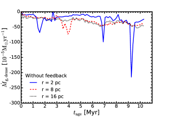
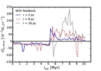
Figure 4: Evolution of the dense gas mass rate of change $\dot{M}_{\rm{\rm g,dense}}$ within spheres of radius $r=$ 2 pc, 8 pc and 16 pc. Run LAF1, with feedback (right panel), shows two clear stages during the first 10 Myr of stellar cluster evolution: a strong collapse stage at the beginning ($\dot{M}_{\rm{\rm g,dense}}<0$, $\it{gas\ accretion}$), and a gas removal stage once stellar feedback becomes important ($\dot{M}_{\rm{\rm g,dense}}>0$).

3.6 Evolution of the star formation rate

The effect of the feedback on the SFR is one of the fundamental questions in the problem of how star formation self-regulates. In the top panel of Fig. 5 we show the evolution of the star formation rate as defined by the second term of the right-hand side of eq. (5), using a sufficiently large radius $r$ to encompass all of the star formation in region SFRegG2 in the two simulations. In both runs, the SFR is extremely intermittent (bursty) over the entire evolution. However, in the feedback run LAF1, the SFR first increases with time, reaching a maximum at $t_{\rm age}\approx 4.5$ Myr, and then it begins to decrease on average, until dense gas is depleted and star formation is fully quenched in the region. Instead, in the non-feedback run LAF0, as long as gas accretion goes on, the SFR continues to grow in time, and reaches higher values than in run LAF1. By the final time shown, $t_{\rm age}\sim 10$ Myr, the mass in stars in region SFRegG2 in run LAF0 is $\sim 2.3$ times larger than the corresponding mass in run LAF1 and is still increasing (see the right panel of Fig. 3), while it has stopped incrreasing in run LAF1, and the SFR has shut off (Fig. 5). The situation is essentially the same for the central group G2 only (middle panel in Fig. 5). This is because most of the star formation activity in the whole SFRegG2 occurs in the clump that gives rise to G2. Specifically, $\sim 87\%$ and 91% of the total mass in stars within SFRegG2 were formed in G2 after 10 Myr of evolution in runs LAF1 and LAF0, respectively.

Figure 5: Instantaneous star formation rate ${\rm SFR}_{t}$ as a function of time for (from top to bottom): the star forming region around G2 (SFRegG2, $\rm{r}<$ 20pc), the G2 group, and for the four subgroups formed farthest from G2 (see Figure 2). It does not matter if we consider the whole region around G2 (SFRegG2) or just the inner four parsecs around G2, ${\rm SFR}_{t}$ increases with time peaking $\sim$5 Myr after the first star was formed, then it decreases; and clearly the non-feedback run (dashed lines) are forming stars at a higher rate than the respective regions in the run that include ionising feedback from massive stars (solid lines). ${\rm SFR}_{t}$ for the subgroups (bottom panel) shows that sometimes feedback just stops the formation of stars (see subG2 and the respective curve for the simulation without feedback), and sometimes it triggers SF, as is the case for subG6, which does not even have a counterpart in the simulation without feedback.

The difference in stellar mass between the two runs (a factor $\sim 2.3$) by the final times ($t_{\rm age}\sim 10$ Myr) shown in Fig. 3 may seem too low to provide any effective self-regulation of star formation. However, what happens is that, in the non-feedback run, star formation continues for a long time after the last times shown in this figure, as can be inferred by the fact that the stellar mass is not only still increasing in run LAF0 at that time, but it is doing so at an accelerated pace. Instead, SF has been almost completely quenched by the feedback at this time in run LAF1, and no new stars are forming in the region. But, comparing the gas and stellar masses at $t_{\rm age}=7$ Myr, at which these masses are still similar in the two simulations, we see that the instantaneous star formation efficiency,

$${\rm SFE}(t)=\frac{M_{\rm S}(t)}{M_{\rm dense}(t)+M_{\rm S}(t)},$$ (6)

is $\approx 4\%$ in LAF1 and $\approx 6.5\%$ in LAF0, since $M_{\rm dense}\approx 5800M_{\odot}$ in both runs, while $M_{\rm S}\approx 250M_{\odot}$ in LAF1 and $M_{\rm S}\approx 400M_{\odot}$ in LAF0. So, at this time, the SFE is still quite low in the two simulations, and consistent with observations. This is due to the multi-timescale nature of the hierarchical collapse and the corresponding acceleration of SF (Vázquez-Semadeni et al., 2019). In order for the non-feedback run LAF0 to more thoroughly convert its gas to stars, significantly longer timescales would be required. The bottom panel of Fig. 5 shows the evolution of the SFR for the stellar subgroups formed within SFRegG2 (cf. Sec. 3.4) but clearly separate from G2 at almost all times. As is the case for the whole G2 cluster, SF is quenched in most of the subgroups in the feedback simulation LAF1. This is exemplified by the curve for subG2, which indicates that SF is halted in this subgroup at $t_{\rm age}\approx 7$ Myr, which corresponds to $\sim 2$ Myr after feedback starts to sweep the gas out from the central region (see the solid magenta line in the left panel of Fig. 3). Thus, the quenching of SF is dominated by the feedback from the most massive star, and, for more distant groups, quenching begins once the expanding shell around that star has engulfed the region containing each group.

3.7 Cluster expansion

At the same time when SF is quenched in subG2 ($t_{\rm age}\approx 7$ Myr), the right panel of Fig. 2 shows that the stars in this group (magenta dots) begin to expand. This is therefore clearly an effect of the removal of the gravitational potential of the gas from the group, because the group has existed since $\sim 4$ Myr before, so that most of its stars are already in place, and it does not expand much at all in the non-feedback run LAF0. The same effect occurs for all other secondary sites, and so, as can be seen from the right panel of Fig. 2, the combined expanding motions of the main group and the subgroups produce a net expansion of the cluster, but not as a simple radial expansion from the central star-forming region, but rather as a hierarchical expansion, resulting from the combined expansion of all groups.

Additionally, the group indicated by the circles in Fig. 1, which is represented by the red dots in both panels of Fig. 2, is seen to completely fall onto the center of mass by $t_{\rm age}\approx 10$ Myr in run LAF0, while its members remain at an average distance of $\approx 2$ pc from the center of mass in run LAF1. This is a pre-gas-removal effect, since in this case, the gas clump is first pushed away from its infall path by the passing expanding shell and then it forms stars. Therefore, in general, the expansion of the cluster is the combined result of two effects: one is the well known effect of the removal of the remaining gas in regions that have already formed most stars, reducing the gravitational potential after it has formed stars. In fact, the feedback may even cause accumulation of gas in the outskirts of the SF region, creating a new potential well that could pull the stars towards these new locations, a mechanism which Zamora-Avilés et al. (2019b) referred to as gravitational feedback; however, we do not see an accumulation of dense gas in the periphery of the cluster in our simulation that could cause such an effect. The second is the indirect injection of momentum to the stars by the feedback, which injects momentum to the gas from which the stars form, so that they inherit their motion from the gas.

3.8 Triggering versus inhibition

An important question about the feedback is whether and to what extent is trigger subsequent star formation episodes in nearby regions, as originally proposed by Elmegreen & Lada (1977). In relation to this question, we focus on the formation of group subG6 (green dots in the right panel of Fig. 2) in run LAF1. This group has no counterpart in the non-feedback run. This group forms at a distance $\sim 9$ pc from G2 and at a time $t_{\rm age}\sim 7.6$ Myr ($\sim 2.6$ Myr after feedback started affecting gas and stars in the central parsec of G2). An animation of the LAF1 run (not shown) shows that, as the expanding shell collides with another infalling filamentary stream, a locally gravitationally unstable clump forms, giving birth to subG2. However, this is the only instance of stimulated star formation we have found in the simulation with feedback, suggesting that this is not the dominant mode of secondary star formation. Instead, all the other subgroups form also in the non-feedback run, indicating that their appearance was not triggered by the feedback from the main hub, but rather was just the manifestation of the small-scale, low-mass peripheral collapsing regions in the GHC process. In this sense, triggering in our simulation appears to be the exception rather than the rule. This seems qualitatively opposite to what was reported by Dale et al. (2012), who found that the negative effect of feedback may be compensated by the positive feedback in the form of triggered SF. We do not find such balance in our simulations. The reason for the disagreement is not clear at the moment, although it may be at least partly due to the very different morphology of our clouds and theirs, since ours are flattened due to their formation mechanism through the collision of streams, while theirs are not formed self-consistently, but initially set up as spherical clouds. In any case, a detailed comparison is in order, which we hope to carry out in a future contribution.

More recently, Bending et al. (2020) studied the role of photoionization feedback on large spiral arms environment, finding that the feedback causes the formation of larger masses of dense gas, and a period of increased star formation than in a simulation with no feedback, although the dense gas is more scattered, and ultimately they report a lower overall SFR. In our case, we do not see the formation of much additional dense gas, although this may be an artifact of our simplified radiative transfer scheme. We plan to perform detailed comparisons with simulations using full radiative transfer to evaluate the long-term impact of our scheme.

4 Discussion

4.1 Implications

The results presented in the previous section have a number of implications for the study and understanding of the structure and evolution of young stellar clusters. These can be summarized as follows:

First, our finding that most of the secondary star formation sites in the periphery of the main hub are primordial rather than triggered suggests that the vast body of star-forming sites that are proposed as the result of triggering (e.g., Elmegreen & Lada, 1977; Peng et al., 2010; Samal et al., 2014; Ochsendorf et al., 2015; Duronea et al., 2017; Rugel et al., 2019; Panwar et al., 2019, see also the review by Elmegreen 2011 and references therein) may actually contain a large fraction of cases where the star-formation activity would have occurred anyway, with no need for triggering. The GHC scenario implies that the star-forming sites in the clouds exhibit a hierarchical nesting, in which a main star-forming hub is expected to be surrounded by lower-mass star-forming sites (Vázquez-Semadeni et al., 2009; Vázquez-Semadeni et al., 2019). Since the main hub eventually produces massive stars, the Hii regions they produce will eventually engulf the lower-mass sites, and appear as if their star-forming activity may have been triggered by the expanding shells. Although we do not include supernovae in our simulation, a similar effect is expected to occur for cases where the trigger appears to be a supernova explosion (e.g., Kounkel et al., 2018). These authors note that proper motions in the $\lambda$ Ori region imply a radial expansion, and that the traceback age of this expansion exceeds the age of the youngest stars near the outer edges of the region. They thus conclude that the formation of those stars may have been triggered by a supernova explosion when their parent regions were at half their present distance from the cluster centre. According to our results, the triggering is not indispensable, and the stars likely could have formed at that location even without the passage of a shell.

In addition, according to our results, the most important effect of the passage of an expanding shell through a secondary star-forming site is the removal of most of its gas, with the corresponding triggering of the expansion of the stars already formed there. Thus, we propose that, for sub-groups undergoing local expansion, the local traceback age of the sub-group may indicate the time of the shell passage, rather than being an indication of a triggering event.

Finally, our result that the gas mass in the whole region increases faster by accretion than it decreases by conversion to stars has the unexpected implication that part of the observed smallness of the SFE, as defined in eq. (6) is not entirely due to a low rate of conversion to stars, but also to the fact that the star-forming regions themselves are accreting mass from their environment, keeping the ratio in the right-hand side of eq. (6) low. This is a crucial implication of the accretion at all scales in molecular clouds expected to occur in the GHC scenario (Vázquez-Semadeni et al., 2019).

4.2 Comparison with previous work

The evolution of clouds and their star formation activity in the GHC scenario incorporates features of various models previously presented in the literature. The fundamental premise of the GHC scenario (Vázquez-Semadeni et al., 2019) is that the clouds are evolving in near pressure-less collapse, because they contain a large number of Jeans masses. Nevertheless, the clouds do contain moderately supersonic turbulent motions which cause nonlinear density fluctuations. Therefore, the collapse is extremely non-homologous, and regions of different density evolve on their respective collapse timescales. These timescales are, however, longer than the standard free fall time, $t_{\rm ff}=3\pi/(32G\rho)$, because strongly anisotropic objects collapse on timescales longer than $t_{\rm ff}$ by factors that depend on the aspect ratio (Toalá et al., 2012; Pon et al., 2012). Since the collapse is nearly pressureless, anisotropies are amplified, producing filamentary accretion flows that feed the main star-forming hubs, although secondary, lower-mass star formation occurs along the filaments as they become locally Jeans unstable (Gómez & Vázquez-Semadeni, 2014). These filaments are thus “conveyor-belt” type of flows, as proposed by Longmore et al. (2014).

In addition, the primary star formation activity in the hubs and the secondary activity in the filaments leads to a hierarchical process of star formation, in which various groups are formed, thus being analogous to the hierarchical cluster formation proposed by a number of groups (e.g., Fellhauer et al., 2009; Grudić et al., 2018b). Our simulations are complementary to those of the latter authors, because, on the one hand, we consider a self-consistent formation and turbulent driving of the clouds and stellar particles that represent individual stars, while they considered initially spherical, rotating gas configurations, and their sink particles represent stellar groups. On the other hand, those authors considered a wide rang of cloud column densities, while we consider only one case, corresponding to Solar-neighborhood-type clouds. In particular, Grudić et al. (2018b) considered many cases of densities so high that photoionising radiation alone is unable to destroy the clouds, a case we do not encounter in our LAF1 simulation.

The GHC scenario represented by our simulations also implies an acceleration of the star formation process, due to the global gravitational contraction, with the corresponding increase of the mean cloud density and decrease of the mean free-fall time (Zamora-Avilés & Vázquez-Semadeni, 2014; Vázquez-Semadeni et al., 2019). The conclusion of an increasing SFR has also been reached by Lee et al. (2015); Murray & Chang (2015); Caldwell & Chang (2018), although Murray & Chang (2015) specifically suggest that the increase is due to local rather than global collapse, arguing that there is no observational evidence for global, cloud-scale collapse provided by P Cygni profiles toward GMCs on scales larger than $\sim 10$ pc. As discussed in Vázquez-Semadeni et al. (2019), we emphasize that, according to the GHC scenario, the infall does not occur with a near-spherical geometry and thus should be not searched by line-of-sight accretion tracers such as P Cygni profiles, but rather through filamentary accretion flows, and these are routinely observed now on scales up to 10 pc or more (e.g., Schneider et al., 2010; Kirk et al., 2013; Peretto et al., 2014; Tackenberg et al., 2014; Hacar et al., 2017; Chen et al., 2019). The larger-scale accretion flow from cloud to filaments, suggested by the simulations (Gómez & Vázquez-Semadeni, 2014) is indeed more elusive, because it occurs on lower-density gas for which the gravitational velocity is lower, and thus more “polluted” by the turbulent background (Camacho et al., 2016), but nevertheless a global velocity offset between peripheral ¹²CO and internal ¹³CO has been detected for a number of clouds by Barnes et al. (2018).

Concerning the SFE, it has been measured in other numerical works for MCs of similar gas mass ($10^{4}$ $M_{\odot}$) to that of our clouds, but with somewhat different results. For example Dale (2017) also finds SFEs that increase with time, but reaching significantly larger values than we find here. A possible reason, which we plan to explore in the future, is that his simulations start with spherical clouds, while our clouds acquire a sheetlike morphology, due to their formation by the collision of streams. This implies that our clouds produce a much shallower potential well than if their mass were assembled in a roughly spherical configurations.

It is also important to note that different definitions for SFE are used in different works, and care must be taken to ensure that comparisons are meaningful. For instance, Geen et al. (2018) report “total” SFEs, with values in the range of 6-15 %. To compute this total SFE, they take into account the total initial mass in gas. Thus, to make a more adequate comparison, we can use the maximum mass in dense gas attained by SFReg2 throughout its evolution. In this case, the SFE in our simulation is $\sim$ 9% when measured 5 Myrs after feedback started to disperse the gas, a similar value to that reported by Geen et al. (2018).

Our result of a quick destruction of the molecular cloud after the first very massive star appears is consistent with the result by Kim et al. (2018) that the destruction of a MC occurs within 2 –10 Myr after the onset of radiation feedback. Along similar lines, Ali & Harries (2019) reported that, for a MC with $10^{4}$ $M_{\odot}$, 75 percent of its mass is dispersed within 4.3 Myr once a massive star of $\sim$ 34 $M_{\odot}$ is placed in the most massive core within the cloud. In our case, this occurs after 5–10 Myr depending of the star forming region within the numerical box. Similarly, Dale et al. (2012) found that photoionisation disperses the neutral gas around 3 Myr before the explosion of the first supernovae in clouds of mass $10^{4}$–$10^{5}$ $M_{\odot}$. Kim et al. (2018) also report that neutral gas is ejected at a typical velocity of $\sim 6$-15 ${\rm km~{}s}^{-1}$. Although we do not track the velocity of the dense gas directly, we do find (Sec. 3.5) that the dense gas is removed from the region at a velocity $\approx 11$ ${\rm km~{}s}^{-1}$ from the position of the massive star.

In relation to observations, it is interesting to cast our results in the context, for example, of those by Ginsburg et al. (2016). These authors found that, in the W51 massive proto-custer clumps, the feedback from massive stars may be insufficient to halt star formation in the clumps, but may be capable of shutting off the large-scale accretion onto them. Although our star-forming hub SFRegG2 is not as massive, the images of Fig. 1 suggest that indeed the fueling of the hub is destroyed earlier than the hub itself (see the second and third panels from the top on the right column), suggesting a similar mechanism.

Our numerical results are also consistent with the timeline of GMC evolution found observationally by Chevance et al. (2020) in the PHANGS-ALMA survey (Leroy et al., in prep.), finding that GMCs disperse within 1-5 Myr once massive stars emerge. As seen in Figs. 1 and 3, the gas within 20 pc of SFRegG2 is dispersed within $\sim 5$ Myr in our simulation. Moreover, Chevance et al. (2020) also conclude that the total lifetime of GMCs is 10–30 Myr, and their final integrated star formation efficiency is 4–10%. Our simulation results are fully consistent with these numbers: the lifetime of the cloud is $\la 30$ Myr, as can be seen from the fact that the first star forms at $t\sim 19$ Myr after the beginning of the simulations, the first destructive massive star appears $\sim 5$ Myr after the first star, and the cloud is destroyed $\sim 5$ Myr after that, for a total of $\sim 30$ Myr of evolution. This is an upper limit to the cloud’s lifetime, since the cloud becomes massive enough to be considered a GMC some $\sim 10$ Myr after the start of the simulation. Thus, a better estimate of the lifetime of our cloud is $\sim 20$ Myr, fully within the range found by Chevance et al. (2020). Also, the final SFE of our cloud is $\sim 5\%$, also fully within the range of their findings. We conclude that our simulation if fully consistent with their observational constraints.

4.3 Caveats

Although our simulations have the big advantage of forming stellar particles with masses of individual stars thanks to our probabilistic star formation prescription, the mass sampling of the IMF does not reach the low-mass part of the IMF, since the minimum stellar mass we have is $\sim 0.3$ $M_{\odot}$, imposed by our numerical resolution. For a typical IMF, about half of the total stellar mass is in stars with $M<3$ $M_{\odot}$. It is not clear, however, whether our simulation is missing that amount of mass, or has deposited it into the stellar mass range it develops. In any case, the stars that do form have the correct mass distribution, and thus the cluster $N$-body dynamics can be trusted. Moreover, in regards to the effect of momentum injection to the stellar component via the gas while it is forming stars, if the effect is efficient for the higher-mass stars, it should be even more so for the lower-mass ones. Finally, regarding the total amount of energy injected, this does not depend on the lower-mass stars. Thus, we conclude that our results should not be seriously affected by our star-formation prescription, and is anyway more accurate than schemes in which the sink particles have masses corresponding to small clusters.

The other important caveat is the usage of our strongly simplified prescription for injecting the feedback energy. Although in Paper I we presented a test of the method in the standard problem of the expansion of an Hii region in a uniform medium, showing that the numerical solution was always within $\sim 30\%$ of the analytical solution. In addition, the fact that our results are in qualitative agreement with those of other groups, as discussed in Sec. 4.2, suggests that our implementation captures the essential physics. Nevertheless, it is clear that our method has limitations, and we intend to test our results in a forthcoming paper using a full radiative-transfer simulation with the probabilistic star formation prescription.

Finally, it is worth mentioning that we have analysed only one out of the three stellar clusters formed in the numerical box. It would certainly be desirable to have a large sample of simulated star-forming regions with different properties to perform a statistical analysis and test our conclusions. Unfortunately, the study presented in this paper could not be done in automated form, and had to be done manually, because it was necessary to keep track of each star’s position even if it had migrated far from its birthplace (perhaps near another group, so that standard grouping algorithms could not be used), while simultaneously assigning the correct membership to the newly-formed stars, which required a constant updating of the definition of a group. A comprehensive analysis of a large sample of clusters will require first an automatization of the entire procedure.

5 Summary and conclusions

In this paper, we have used two hydrodynamical simulations of MCs undergoing global hierarchical collapse (GHC), with and without feedback (LAF1 and LAF0, respectively), to investigate the effects of the feedback on the shaping of the cluster, removal of the dense gas, and the primordial or triggered nature of the peripheral star formation activity. We focus on a region in the simulation labeled SFRegG2, which contains approximately $10^{4}$ $M_{\odot}$ in dense gas, and which forms stars in a hierarchy consisting of a main hub, denoted G2, and several peripheral subgroups. A key ingredient of our numerical simulations is the sub-grid model for star formation, which allows the stellar particles to have realistic stellar masses, with a Salpeter slope, in the range 0.39–61 $M_{\odot}$, with each star feeding back at the rate corresponding to its mass. This allows us to have a realistic implementation of feedback from massive stars, and also a realistic description of the cluster dynamics.

We found that the evolution of the two simulations is quite similar until a very massive ($M\approx 30$ $M_{\odot}$) forms, at $t_{\rm age}\sim 5$ Myr after the formation of the first star in the cluster. After that time, the expansion of the Hii region formed by this star dominates the dynamics of both the gas and the stars in the region, causing the feedback run to behave very differently from the non-feedback one. Our main results are as follows:

• Because gas is funneled to the star-forming hubs and cores by the filaments, the amount of material available for forming the most massive stars is also limited, causing the most massive stars in run LAF1 to be less massive than the corresponding ones in run LAF0. Also, these most massive stars in run LAF0 appear at a later time than their less massive counterparts in LAF1, suggesting that more massive, denser clumps are necessary to form more massive stars.

• Before the feedback from the very massive star begins to dominate, the mass accretion rate onto the star-forming region SFRegG2 is larger than the rate of gas consumption by star formation, so that the mass and density of the region increase, and the measured instantaneous SFE given by eq. (6) remains low, in spite of the star formation activity occurring with virtually no opposition from feedback.

• Most of the peripheral, low-mass star-forming sites form also in the non-feedback run LAF0, indicating they are of a primordial nature, rather than triggered by the passage of the expanding shell of the Hii region. We have found only one case of truly triggered star formation (i.e., a star forming site that occurs in the feedback run but not in the non-feedback one), out of a total of 6 peripheral regions. This also implies that the net effect of the feedback on the SFR is to quench it, although locally it is possible to find examples of triggering.

• After feedback begins to dominate, the dense gas is removed from the star-forming region SFRegG2 at a velocity $\approx 11\ \rm{km\ seg}^{-1}$, as indicated by the times at which the dense gas mass contained within successively larger spheres around the central hub begins to decrease. The net flux of dense gas becomes outwards-directed, as shown in Fig. 4, reversing the previous trend of the hub’s mass increasing faster by accretion than it could consume its mass by star formation. During this stage, both the gas mass and the SFR in the region begin to decrease, although the onset of this decrease “propagates” outwards at the ejection velocity. Therefore, secondary star-forming sites in the periphery of the hub begin to lose their gas and reduce their SFR later than the central hub.

• The spatial and kinematic structure of the stellar component is also strongly affected by the feedback, and not only because of the reduction of the local potential well caused by the removal of the dense gas. An important simultaneous mechanism is the injection of momentum to the star-forming gas in the peripheral sites by the expanding shell. In the non-feedback run, these sites are generally falling onto the main hub along the filaments, but the passage of the expanding shell partially counteracts this motion, reducing or reverting the infall. Therefore, the subgroups end up not having very large infall speeds towards the main hub, and instead have smaller, more random velocities.

• The two previous results remove the concern about the GHC scenario raised by Krumholz et al. (2019, Sec. 3.4.1), that the stellar motions should be directed radially inwards before gas is expelled, and outwards after gas is removed. This criticisms arises from an oversimplification of the GHC scenario, ignoring its hierarchical nature and picturing it as a globally monolithic collapse. Our simulations show that the combination of the scattered nature of the hierarchical star formation region, with a main hub and several secondary neighboring sites, together with the “braking” of the infall by the pressure of the dominant Hii region implies that: a) There is no strong global radial motion of the subgroups in relation to the central hub before the gas removal, and b) According to the discussion in Sec. 3.7, after each subgroup begins to lose its gas, the locally dominant expansion motion is with respect to its local center, not with respect to the main hub. The cluster as a whole expands as well, but as a consequence of the local expansion of each group, not as a coherent expansion from the central hub. Therefore, the resulting motions are much more moderate than estimated by Krumholz et al. (2019) under the assumption of a monolithic, rather than hierarchical, cloud collapse, and thus the resulting concerns are not applicable to GHC.

Data availability

The data underlying this article will be shared on reasonable request to the corresponding author.

References

- Ali & Harries (2019) Ali A. A., Harries T. J., 2019, MNRAS, 487, 4890
- Audit & Hennebelle (2005) Audit E., Hennebelle P., 2005, A&A, 433, 1
- Ballesteros-Paredes et al. (1999a) Ballesteros-Paredes J., Vázquez-Semadeni E., Scalo J., 1999a, ApJ, 515, 286
- Ballesteros-Paredes et al. (1999b) Ballesteros-Paredes J., Vázquez-Semadeni E., Scalo J., 1999b, ApJ, 515, 286
- Barnes et al. (2018) Barnes P. J., Hernandez A. K., Muller E., Pitts R. L., 2018, ApJ, 866, 19
- Bate (2009) Bate M. R., 2009, MNRAS, 392, 1363
- Baumgardt & Kroupa (2007) Baumgardt H., Kroupa P., 2007, MNRAS, 380, 1589
- Bending et al. (2020) Bending T. J. R., Dobbs C. L., Bate M. R., 2020, MNRAS, 495, 1672
- Bressan et al. (1993) Bressan A., Fagotto F., Bertelli G., Chiosi C., 1993, Astronomy and Astrophysics Supplement Series, 100, 647
- Caldwell & Chang (2018) Caldwell S., Chang P., 2018, MNRAS, 474, 4818
- Camacho et al. (2016) Camacho V., Vázquez-Semadeni E., Ballesteros-Paredes J., Gómez G. C., Fall S. M., Mata-Chávez M. D., 2016, ApJ, 833, 113
- Chen et al. (2019) Chen H.-R. V., et al., 2019, ApJ, 875, 24
- Chevance et al. (2020) Chevance M., et al., 2020, MNRAS, 493, 2872
- Colín et al. (2013) Colín P., Vázquez-Semadeni E., Gómez G. C., 2013, MNRAS, 435, 1701
- Colling et al. (2018) Colling C., Hennebelle P., Geen S., Iffrig O., Bournaud F., 2018, A&A, 620, A21
- Da Rio et al. (2017) Da Rio N., et al., 2017, ApJ, 845, 105
- Dale (2015) Dale J. E., 2015, New Astron. Rev., 68, 1
- Dale (2017) Dale J. E., 2017, MNRAS, 467, 1067
- Dale et al. (2012) Dale J. E., Ercolano B., Bonnell I. A., 2012, MNRAS, 424, 377
- Dale et al. (2013) Dale J. E., Ercolano B., Bonnell I. A., 2013, MNRAS, 430, 234
- Dale et al. (2014) Dale J. E., Ngoumou J., Ercolano B., Bonnell I. A., 2014, MNRAS, 442, 694
- Diaz-Miller et al. (1998) Diaz-Miller R. I., Franco J., Shore S. N., 1998, ApJ, 501, 192
- Duronea et al. (2017) Duronea N. U., Cappa C. E., Bronfman L., Borissova J., Gromadzki M., Kuhn M. A., 2017, A&A, 606, A8
- Elmegreen & Lada (1977) Elmegreen B. G., Lada C. J., 1977, ApJ, 214, 725
- Fellhauer et al. (2009) Fellhauer M., Wilkinson M. I., Kroupa P., 2009, MNRAS, 397, 954
- Geen et al. (2018) Geen S., Watson S. K., Rosdahl J., Bieri R., Klessen R. S., Hennebelle P., 2018, MNRAS, 481, 2548
- Ginsburg et al. (2016) Ginsburg A., et al., 2016, A&A, 595, A27
- Gómez & Vázquez-Semadeni (2014) Gómez G. C., Vázquez-Semadeni E., 2014, ApJ, 791, 124
- Grudić et al. (2018a) Grudić M. Y., Hopkins P. F., Faucher-Giguère C.-A., Quataert E., Murray N., Kereš D., 2018a, MNRAS, 475, 3511
- Grudić et al. (2018b) Grudić M. Y., Guszejnov D., Hopkins P. F., Lamberts A., Boylan-Kolchin M., Murray N., Schmitz D., 2018b, MNRAS, 481, 688
- Hacar et al. (2016) Hacar A., Alves J., Forbrich J., Meingast S., Kubiak K., Großschedl J., 2016, A&A, 589, A80
- Hacar et al. (2017) Hacar A., Alves J., Tafalla M., Goicoechea J. R., 2017, A&A, 602, L2
- Haid et al. (2018) Haid S., Walch S., Seifried D., Wünsch R., Dinnbier F., Naab T., 2018, MNRAS, 478, 4799
- Haid et al. (2019) Haid S., Walch S., Seifried D., Wünsch R., Dinnbier F., Naab T., 2019, MNRAS, 482, 4062
- Heitsch et al. (2005) Heitsch F., Burkert A., Hartmann L. W., Slyz A. D., Devriendt J. E. G., 2005, ApJ, 633, L113
- Heitsch et al. (2006) Heitsch F., Slyz A. D., Devriendt J. E. G., Hartmann L. W., Burkert A., 2006, ApJ, 648, 1052
- Heitsch et al. (2008) Heitsch F., Hartmann L. W., Slyz A. D., Devriendt J. E. G., Burkert A., 2008, ApJ, 674, 316
- Heitsch et al. (2009) Heitsch F., Ballesteros-Paredes J., Hartmann L., 2009, ApJ, 704, 1735
- Hennebelle & Pérault (2000) Hennebelle P., Pérault M., 2000, A&A, 359, 1124
- Hennebelle et al. (2008) Hennebelle P., Banerjee R., Vázquez-Semadeni E., Klessen R. S., Audit E., 2008, A&A, 486, L43
- Iffrig & Hennebelle (2015) Iffrig O., Hennebelle P., 2015, A&A, 576, A95
- Iffrig & Hennebelle (2017) Iffrig O., Hennebelle P., 2017, A&A, 604, A70
- Inoue et al. (2006) Inoue T., Inutsuka S.-i., Koyama H., 2006, ApJ, 652, 1331
- Kim et al. (2018) Kim J.-G., Kim W.-T., Ostriker E. C., 2018, ApJ, 859, 68
- Kirk et al. (2013) Kirk H., Myers P. C., Bourke T. L., Gutermuth R. A., Hedden A., Wilson G. W., 2013, ApJ, 766, 115
- Körtgen et al. (2016) Körtgen B., Seifried D., Banerjee R., Vázquez-Semadeni E., Zamora-Avilés M., 2016, MNRAS, 459, 3460
- Kounkel et al. (2018) Kounkel M., et al., 2018, AJ, 156, 84
- Koyama & Inutsuka (2000) Koyama H., Inutsuka S.-I., 2000, ApJ, 532, 980
- Koyama & Inutsuka (2002) Koyama H., Inutsuka S.-i., 2002, ApJ, 564, L97
- Koyama & Inutsuka (2004) Koyama H., Inutsuka S.-i., 2004, ApJ, 602, L25
- Kravtsov (2003) Kravtsov A. V., 2003, ApJ, 590, L1
- Kravtsov et al. (1997) Kravtsov A. V., Klypin A. A., Khokhlov A. M., 1997, The Astrophysical Journal Supplement Series, 111, 73
- Krumholz et al. (2019) Krumholz M. R., McKee C. F., Bland -Hawthorn J., 2019, ARA&A, 57, 227
- Lada et al. (1984) Lada C. J., Margulis M., Dearborn D., 1984, ApJ, 285, 141
- Lee et al. (2015) Lee E. J., Chang P., Murray N., 2015, ApJ, 800, 49
- Longmore et al. (2014) Longmore S. N., et al., 2014, in Beuther H., Klessen R. S., Dullemond C. P., Henning T., eds, Protostars and Planets VI. p. 291 (arXiv:1401.4175), doi:10.2458/azu_uapress_9780816531240-ch013
- Matzner (2002) Matzner C. D., 2002, ApJ, 566, 302
- Murray & Chang (2015) Murray N., Chang P., 2015, ApJ, 804, 44
- Ochsendorf et al. (2015) Ochsendorf B. B., Brown A. G. A., Bally J., Tielens A. G. G. M., 2015, ApJ, 808, 111
- Panwar et al. (2019) Panwar N., Samal M. R., Pandey A. K., Singh H. P., Sharma S., 2019, AJ, 157, 112
- Parmentier et al. (2008) Parmentier G., Goodwin S. P., Kroupa P., Baumgardt H., 2008, ApJ, 678, 347
- Peng et al. (2010) Peng T. C., Wyrowski F., van der Tak F. F. S., Menten K. M., Walmsley C. M., 2010, A&A, 520, A84
- Peretto et al. (2014) Peretto N., et al., 2014, A&A, 561, A83
- Pon et al. (2012) Pon A., Toalá J. A., Johnstone D., Vázquez-Semadeni E., Heitsch F., Gómez G. C., 2012, ApJ, 756, 145
- Rey-Raposo et al. (2015) Rey-Raposo R., Dobbs C., Duarte-Cabral A., 2015, MNRAS, 446, L46
- Roberts (1969) Roberts W. W., 1969, ApJ, 158, 123
- Rugel et al. (2019) Rugel M. R., et al., 2019, A&A, 622, A48
- Samal et al. (2014) Samal M. R., et al., 2014, A&A, 566, A122
- Sasao (1973) Sasao T., 1973, PASJ, 25, 1
- Schneider et al. (2010) Schneider N., Csengeri T., Bontemps S., Motte F., Simon R., Hennebelle P., Federrath C., Klessen R., 2010, A&A, 520, A49
- Smith et al. (2009) Smith R. J., Longmore S., Bonnell I., 2009, MNRAS, 400, 1775
- Strömgren (1939) Strömgren B., 1939, ApJ, 89, 526
- Tackenberg et al. (2014) Tackenberg J., et al., 2014, A&A, 565, A101
- Toalá et al. (2012) Toalá J. A., Vázquez-Semadeni E., Gómez G. C., 2012, ApJ, 744, 190
- Tutukov (1978) Tutukov A. V., 1978, A&A, 70, 57
- Vázquez-Semadeni (2011) Vázquez-Semadeni E., 2011, in Alves J., Elmegreen B. G., Girart J. M., Trimble V., eds, IAU Symposium Vol. 270, Computational Star Formation. pp 275–282 (arXiv:1010.5157), doi:10.1017/S1743921311000500
- Vázquez-Semadeni et al. (2006) Vázquez-Semadeni E., Ryu D., Passot T., González R. F., Gazol A., 2006, ApJ, 643, 245
- Vázquez-Semadeni et al. (2007) Vázquez-Semadeni E., Gómez G. C., Jappsen A. K., Ballesteros-Paredes J., González R. F., Klessen R. S., 2007, ApJ, 657, 870
- Vázquez-Semadeni et al. (2009) Vázquez-Semadeni E., Gómez G. C., Jappsen A. K., Ballesteros-Paredes J., Klessen R. S., 2009, ApJ, 707, 1023
- Vázquez-Semadeni et al. (2017) Vázquez-Semadeni E., González-Samaniego A., Colín P., 2017, MNRAS, 467, 1313
- Vázquez-Semadeni et al. (2019) Vázquez-Semadeni E., Palau A., Ballesteros-Paredes J., Gómez G. C., Zamora-Avilés M., 2019, MNRAS, 490, 3061
- Vishniac (1994) Vishniac E. T., 1994, ApJ, 428, 186
- Walder & Folini (1998) Walder R., Folini D., 1998, A&A, 330, L21
- Zamora-Avilés & Vázquez-Semadeni (2014) Zamora-Avilés M., Vázquez-Semadeni E., 2014, ApJ, 793, 84
- Zamora-Avilés et al. (2019a) Zamora-Avilés M., et al., 2019a, MNRAS, 487, 2200
- Zamora-Avilés et al. (2019b) Zamora-Avilés M., Ballesteros-Paredes J., Hernández J., Román-Zúñiga C., Lora V., Kounkel M., 2019b, MNRAS, 488, 3406
- von Weizsäcker (1951) von Weizsäcker C. F., 1951, ApJ, 114, 165