Coordinate-free Isoline Tracking in Unknown 2-D Scalar Fields

Abstract

The isoline tracking of this work is concerned with the control design for a sensing robot to track a given isoline of an unknown 2-D scalar filed. To this end, we propose a coordinate-free controller with a simple PI-like form using only the concentration feedback for a Dubins robot, which is particularly useful in GPS-denied environments. The key idea lies in the novel design of a sliding surface based error term in the standard PI controller. Interestingly, we also prove that the tracking error can be reduced by increasing the proportion gain, and is eliminated for circular fields with a non-zero integral gain. The effectiveness of our controller is validated via simulations by using a fixed-wing UAV on the real dataset of the concentration distribution of PM 2.5 in Handan, China.

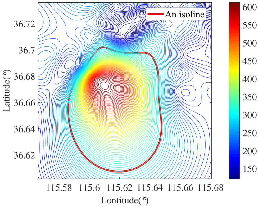
(a)

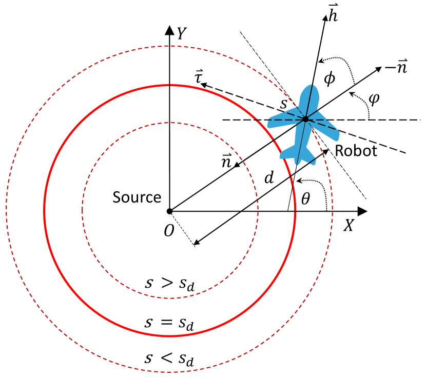
(b)

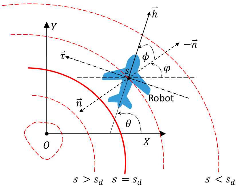
(c)

Figure 1: (a) PM2.5 concentration observed in Handan, a city in North China, at 2018/11/25 22:00:00. (b) Coordinates of the Dubins robot in scalar fields. (c) Coordinates of the Dubins robot in circular fields.

I Introduction

The isoline tracking refers to the tactic that a mobile robot reaches and then tracks a predefined contour in a scalar field, which is widely applied in the areas of detection, exploration, monitoring, and etc. In the literature, it is also named as curve tracking [malisoff2017adaptive], boundary tracking [matveev2017tight, mellucci2019environmental], level set tracking [Matveev2012Method]. In fact, it covers the celebrated target circumnavigation as a special case [deghat2012target, swartling2014collective, dong2020Circumnavigating].

Compared with the static sensor networks, it is more flexible and economical to utilize mobile sensors to collect data or track target. The methods for isoline tracking by robots have been applied to many practical problems, e.g., exploring environmental feature of bathymetric depth [mellucci2019environmental], tracking boundary of volcanic ash [kim2017disturbance], tracking curve of sea temperature [zhang2010cooperative], and monitoring algal bloom[fonseca2019cooperative].

Roughly speaking, we can categorize the methods for isoline tracking depending on whether the gradient of the scalar field can be used or not. The gradient-based method is extensively used to the extreme seeking problem, which steers a robot to track the direction of gradient descending (ascending) to reach the minimizer (maximizer) of a scalar field [zhang2010cooperative, wu2012robust].

If the explicit gradient is not available, many works focus on the problem of gradient estimation, which mainly include two main strategies: (i) a single robot changes its position over time to collect the signal propagation at different locations; and (ii) multiple robots collaborate to obtain measurements at different locations at the same time. For the case (i), Ai et al. [ai2016source] show a sequential least-squares field estimation algorithm for a REMUS AUV to seek the source of a hydrothermal plume. Moreover, the stochastic method for extreme seeking is also gradient-based, the idea behind which is to approximate the gradient of the signal strength and to use this information to drive the robot towards the source by adding an excitatory input to the robot steering control [cochran20093, lin2017stochastic]. For the case (ii), a circular formation of robots is adopted in [brinon2015distributed, brinon2019multirobot] to estimate the gradient of fields. Moreover, a provably convergent cooperative Kalman filter and a cooperative $H_{\infty}$ filter are devised to estimate the gradient in [zhang2010cooperative] and [wu2012robust], respectively.

In many scenarios, robots cannot obtain its position and can only measure the signal strength at the current location of the sensor, i.e., the measurement in a point-wise fashion [Matveev2012Method]. Thus, it is impossible to estimate the field gradient, and researchers turn to exploiting gradient-free methods. A sliding mode approach is proposed for target circumnavigation by [Matveev2011Range] and then is adopted to similar problems, e.g., level sets tracking [Matveev2012Method], boundary tracking [matveev2015robot], etc. Without a rigorous justification, they address the “chattering” phenomenon by modeling dynamics of the actuator as the simplest first order linear differential equation in implementation. A PD controller is devised in [baronov2007reactive] for a double-integrator robot to track isolines in a harmonic potential field. Besides, a PID controller with adaptive crossing angle correction is shown in [newaz2018online]. Furthermore, there are some heuristic methods for isoline tracking, e.g., sub-optimal sliding mode algorithm of [mellucci2017experimental].

In this paper, we propose a coordinate-free controller in a PI-like from for a Dubins robot to track a desired isoline by using only the concentration feedback. That is, we do not use any field gradient or the position of the robot, which renders our controller particularly useful in the GPS-denied environment. Our key idea lies in the novel design of a sliding surface based error term in the standard PI controller. Similar to the standard PI controller, we show that the final tracking error can be reduced by increasing the proportion gain, and is eliminated for circular fields with a non-zero integral gain. For the case of smoothing scalar fields, we explicitly show the upper bound of the steady-state tracking error, which can be reduced by increasing the proportional gain. To validate the effectiveness of our controller, we adopt a fixed-wing UAV to track the isoline of the concentration distribution of PM 2.5 in Handan, China.

The rest of this paper is organized as follows. In Section II, the problem under consideration is formulated in details. Particularly, we clearly describe the desired isoline tracking pattern. To achieve the objective, we propose a PI-like controller for a Dubins robot in Section III. In Section V, we explicitly show the upper bound of the steady-state error in scalar fields. Moreover, we show that the isoline tracking system is locally exponentially stable in Section IV. Simulations are performed in Section LABEL:secsim, and some concluding remarks are drawn in Section LABEL:sec6.

II Problem Formulation

In Fig. 1(a), we provide a 2-D example of the concentration distribution of PM 2.5 in Handan, China on November 25, 2018. In the environmental monitoring, it is fundamentally important to investigate the concentration distribution of air pollutants. To achieve it, we design a sensing robot to track an isoline of its distribution function. Mathematically, the concentration of a 2-D scalar field can be described by

$$F(\bm{p}):\mathbb{R}^{2}\rightarrow\mathbb{R},$$ (1)

where $\bm{p}\in\mathbb{R}^{2}$ is the position. Given a concentration level $s_{d}$, an isoline $\mathcal{L}(s_{d})$ is defined as

$$\mathcal{L}(s_{d})=\{\bm{p}|F(\bm{p})=s_{d}\}.$$ (2)

The isoline tracking problem is on the design of a controller for a sensing robot to reach a given isoline and maintain on the isoline with a constant speed. That is, the objective is to asymptotically steer a sensing robot such that

$$\lim_{t\rightarrow\infty}|s(t)-s_{d}|\rightarrow 0~{}\&~{}\|\dot{\bm{p}}(t)\|=v,$$ (3)

where $s(t)=F(\bm{p}(t))$ is the concentration measurement of the scalar field at the GPS position $\bm{p}(t)$ of the robot and $v$ is its constant linear speed. For a circular field, e.g., acoustic field, then

$$F(\bm{p})=I_{0}\exp(-\varsigma\|\bm{p}-\bm{p}_{o}\|_{2}),$$ (4)

where $\bm{p}_{o}$ is the source position of the field and $I_{0}$, $\varsigma$ are unknown parameters. The isoline tracking in (3) is exactly reduced to the celebrated circumnavigation problem [deghat2012target, swartling2014collective, dong2020Circumnavigating].

In this work, we are interested in the scenario that both the concentration distribution $F(\bm{p})$ and the GPS position of the sensing robot are unknown. Moreover, we cannot measure a continuum of the scalar field, which implies that the gradient-based methods [zhang2010cooperative, malisoff2017adaptive, brinon2019multirobot] cannot be applied here.

III Controller Design

In this section, we design a coordinate-free controller in a PI (proportional integral)-like form for a Dubins robot to complete the isoline tracking problem. The key idea lies in the novel design of a sliding surface based error term in the standard PI controller.

III-A The PI-like controller for a Dubins Robot

Consider a Dubins robot on a 2-D plane

$$\dot{\bm{p}}(t)=v\begin{bmatrix}\cos\theta(t)\\ \sin\theta(t)\end{bmatrix},~{}~{}\dot{\theta}(t)=\omega(t),$$ (5)

where $\bm{p}(t)=[x(t),y(t)]^{\prime}$, $\theta(t)$, $\omega(t)$ and $v$ are the position, heading course, the tunable angular speed and constant linear speed, respectively.

To achieve the objective in (3) by the Dubins robot (5), we propose a novel PI-like controller

$$\omega(t)=k_{p}e(t)+k_{i}\sigma(t),$$ (6)

where $\dot{\sigma}(t)=e(t)$, $k_{p}>0$ and $k_{i}\geq 0$ are the control parameters to be designed.

Let the tracking error be $\varepsilon(t)=s(t)-s_{d}$. The major difference of (6) from the standard PI controller lies in the novel design of the following error term

$$e(t)=\dot{\varepsilon}(t)+c_{1}\tanh\left({\varepsilon(t)}/{c_{2}}\right),$$ (7)

where $c_{1,2}>0$ are constant parameters, and $\tanh(\cdot)$ is the standard hyperbolic tangent function to ensure that the selection of the control parameters is independent of the maximum range of the operating space of the controller. In fact, the error term $e(t)$ in (7) can also be regarded as a sliding surface. For example, once reaching the surface, i.e., $e(t)=0$, it follows that

$$\dot{\varepsilon}(t)=-c_{1}\tanh\left(\varepsilon(t)/c_{2}\right),$$

which further implies that $\varepsilon(t)$ will tend to zero with an exponential convergence speed, i.e., the robot will eventually reach the isoline $\mathcal{L}(s_{d})$.

Intuitively, the PI-like controller (6) consists of two terms: (i) the proportional term for global stability, and (ii) the integral term to eliminate the steady-state error. Similar to the standard PI controller, the integral coefficient $k_{i}$ is generally much smaller than the proportional coefficient $k_{p}$. It is worth mentioning that $c_{1}$ affects the convergence speed and $c_{2}$ affects the sensitivity to the tracking error $\varepsilon(t)$.

Clearly, the PI-like controller (6) of this work only uses the concentration measurement $s(t)$ of the scalar field, and is particularly useful in GPS-denied environments.

III-B Comparison with the existing methods

Some related methods to our proposed control laws are (i) the sliding mode controller in [Matveev2012Method], (ii) the PD controller in [baronov2007reactive], and (iii) the sliding mode controller with two-sliding motions in [mellucci2019environmental]. The sliding mode approach in [Matveev2012Method] is originally designed for the problem of target circumnavigation [Matveev2011Range] with range-based measurements, and then is adopted to isoline tracking in [Matveev2012Method]. Besides the existence of the chattering phenomenon, their method cannot achieve zero steady-state error even for the task of circumnavigation. In contrast, our PI-like controller (6) is continuous and particularly useful to isoline tracking in circular fields, since the integral part can exactly eliminate the steady-state error. Moreover, the PD feedback controller in [baronov2007reactive] is devised for a double-integrator robot, and their control parameters depend on maximum range of the controller operating space. We address this issue by introducing a hyperbolic tangent function $\tanh(\cdot)$. Furthermore, the controller in [mellucci2019environmental] needs two-sliding motions. They validate their controller by both simulations in a synthetic data-based environment and sea-trials by a C-Enduro ASV in Ardmucknish Bay off Dunstaffnage in Scotland. However, their method is heuristic and in fact only offers uncompleted justification.

$$Q=\begin{bmatrix}&k_{p}\alpha v\mu_{1}^{2}-\displaystyle\frac{k_{i}c_{1}\alpha\mu_{1}}{c_{2}}&0&0\\ &0&(k_{p}\alpha v)^{3}&\displaystyle k_{i}(k_{p}\alpha v)^{2}-k_{i}^{2}\alpha v/2+\frac{k_{p}k_{i}c_{2}(\alpha v)^{2}\mu_{1}}{c_{1}\alpha}\\ &0&\displaystyle k_{i}(k_{p}\alpha v)^{2}-k_{i}^{2}\alpha v/2+\frac{k_{p}k_{i}c_{2}(\alpha v)^{2}\mu_{1}}{c_{1}\alpha}&k_{p}k_{i}^{2}\alpha v\end{bmatrix}$$ (17)

IV Isoline Tracking in Circular Fields

In this section, we first consider the case of a circular field in (4). Taking logarithmic function on both sides of (4), there is no loss of generality to write it in the following form

$$F(\bm{p})=s_{d}-\alpha(d(t)-r_{d}),$$ (8)

where $s_{d}$ is the desired isoline, $\alpha\geq\underline{\alpha}$ is an unknown positive constant, $d(t)=\|\bm{p}(t)-\bm{p}_{o}\|_{2}$ is the distance from the robot to the position $\bm{p}_{o}$ of the source, and $r_{d}$ denotes the unknown radius when the robot travels on the desired isoline, i.e., $s(t)=s_{d}$.

Let $\bm{n}=\nabla F(\bm{p})$ denote the gradient vector of $F(\bm{p})$, see Fig. 1(b), and $\bm{h}=[\cos\theta,~{}\sin\theta]^{\prime}$ represent the course vector of the Dubins robot and $\bm{\tau}$ to represent the tangent vector of $\bm{h}$. By convention, $\bm{h}$ and $\bm{\tau}$ form a right-handed coordinate frame with $\bm{h}\times\bm{\tau}$ pointing to the reader.

After converting the coordinates of the robot from the Cartesian frame into the polar frame, we use the concentration $s(t)$ and angle $\phi(t)$ to describe the tracking system. See Fig. 1(c) for illustrations, where $\bm{n}$ exactly points to the source and $\phi(t)$ is formed by the negative gradient vector $-\bm{n}$ and the heading vector $\bm{h}$. The counter-clockwise direction is set to be positive.

By definitions of $s(t)$ and $\phi(t)$, we have that

$$\begin{split}\dot{s}(t)&=-\alpha\dot{d}(t)=-\alpha v\cos\phi(t),\\ \dot{\phi}(t)&=\omega(t)-\frac{v}{d(t)}\sin\phi(t).\end{split}$$ (9)

If $s(t)$ converges to $s_{d}$, then $d(t)$ also converges to $r_{d}$. However, $r_{d}$ is unknown to the sensing robot, which is substantially different from the target circumnavigation problem [deghat2012target, swartling2014collective], and we cannot use the control bias $\omega_{c}=v/r_{d}$ to eliminate the tracking error as in [dong2020Circumnavigating]. To solve it, we design an integral term $k_{i}\sigma(t)$ in (6).

Proposition 1

Consider the tracking system in (9) under the PI-like controller in (6). Define $\bm{x}(t)=[s(t),~{}\phi(t)]^{\prime}$ and $\bm{x}_{e}=[s_{d},~{}-\pi/2]^{\prime}$. If the control parameters are selected to satisfy that

$$k_{p}(k_{p}-2)v\underline{\alpha}>k_{i}~{}\text{and}~{}v\underline{\alpha}>c_{1}>0,$$ (10)

then $\bm{x}_{e}$ is a locally exponentially stable equilibrium of the tracking system (9).

Proof:

By (9), the tracking system under the PI-like controller (6) is written as

$$\begin{split}\dot{d}(t)=&~{}v\cos\phi(t),\\ \dot{\phi}(t)=&~{}-k_{p}\left(\alpha\dot{d}(t)+{c_{1}}\tanh\left({\alpha/c_{2}\cdot(d(t)-r_{d})}\right)\right)\\ &~{}+k_{i}\sigma(t)-{v}\sin\phi(t)/{d(t)},\\ \dot{\sigma}(t)=&-\alpha\dot{d}(t)+{c_{1}}\tanh\left({-\alpha/{c_{2}}\cdot(d(t)-r_{d})}\right).\end{split}$$ (11)

Then, we define an error vector

$$\bm{z}(t) =[z_{1}(t),~{}z_{2}(t),~{}z_{3}(t)]^{\prime}$$

$$=[d(t)-r_{d},~{}\phi(t)+\pi/2,~{}\sigma(t)+v/k_{i}r_{d}]^{\prime},$$

and linearize (11) around $[r_{d},~{}-\pi/2,~{}-v/k_{i}r_{d}]^{\prime}$ as follows

$$\dot{\bm{z}}(t)=A\bm{z}(t),$$ (12)

where the Jacobian matrix $A$ is given by

$$A=\begin{bmatrix}0&v&0\\ -{k_{p}c_{1}\alpha}/{c_{2}}-{v}/{r_{d}^{2}}&-{k_{p}v\alpha}&k_{i}\\ -c_{1}\alpha/c_{2}&-v\alpha&0\end{bmatrix}.$$

Consider a Lyapunov function candidate as

$$V(\bm{z})= ~{}\mu_{2}z_{1}^{2}(t)+\mu_{3}z_{2}^{2}(t)+\mu_{4}z_{3}^{3}(t)$$ (13)

$$+\frac{1}{2}\left(-\mu_{1}z_{1}^{2}(t)-c_{1}v\alpha z_{2}(t)+c_{2}z_{3}(t)\right)^{2},$$

where $\mu_{1}={k_{p}c_{1}\alpha}/{c_{2}}+{v}/{r_{d}^{2}}$, $\mu_{2}=k_{p}\alpha(k_{p}\alpha v\mu_{1}-k_{i}c_{1}\alpha/(2c_{2}))$, $\mu_{3}=\mu_{1}v/2+k_{i}\alpha v/2$, and $\mu_{4}=k_{p}k_{i}c_{2}v\mu_{1}/c_{1}-k_{i}^{2}/2$. It is clear that the conditions in (10) ensure that $V(\bm{z})$ is nonnegative.

Then, we write (13) as the following form

$$V(\bm{z})=\bm{z}^{\prime}P\bm{z},$$ (14)

where

$$P=\frac{1}{2}\begin{bmatrix}2\mu_{2}+\mu_{1}^{2}&k_{p}\alpha v\mu_{1}&-k_{i}\mu_{1}\\ k_{p}\alpha v\mu_{1}&2\mu_{3}+(k_{p}\alpha v)^{2}&-k_{p}k_{i}\alpha v\\ -k_{i}\mu_{1}&-k_{p}k_{i}\alpha v&2\mu_{4}+k_{i}^{2}\end{bmatrix},$$

which leads to that

$$\lambda_{\min}(P)\|\bm{z}\|_{2}^{2}\leq V(\bm{z})\leq\lambda_{\max}(P)\|\bm{z}\|_{2}^{2},$$ (15)

where $\lambda_{\min}(P)$ and $\lambda_{\max}(P)$ denote the minimum and maximum eigenvalues of $P$.

Taking the derivative of $V(\bm{z})$ along with (12) leads to that

$$\dot{V}(\bm{z})=-\bm{z}^{\prime}Q\bm{z},$$ (16)

where $Q$ is shown in (17) and is positive definite by the conditions in (10).

Then, it follows from (15) and (16) that

$$\dot{V}(\bm{z})\leq-\lambda_{\min}(Q)\|\bm{z}\|_{2}^{2}\leq-\frac{\lambda_{\min}(Q)}{\lambda_{\max}(P)}V(\bm{z}).$$ (18)

By the comparison principle [Khalil2002Nonlinear], the tracking system (9) is locally exponentially stable under the PI-like controller (6).

 

(a)

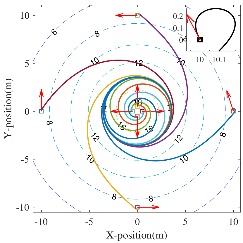
(b)

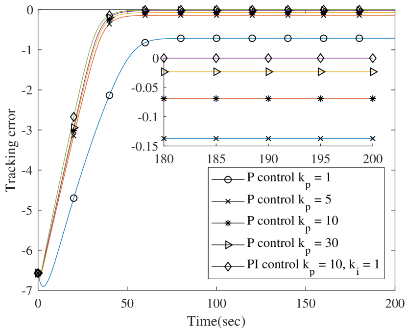
(c)

Figure 2: (a) Fields distribution and trajectory of the Dubins robot. (b) Trajectories of the Dubins robot with different initial states. (c) Tracking errors of the Dubins robot with different control parameters.

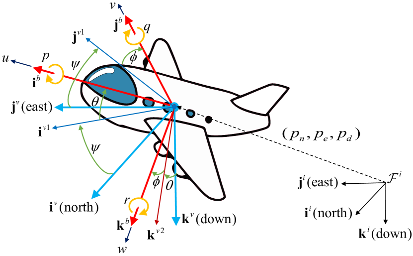
(a)

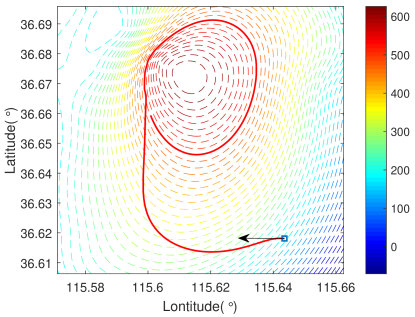
(b)

(c)

Figure 3: (a) Coordinates of a fixed-wing UAV. (b) Trajectory of the fixed-wing UAV in the field of PM2.5. (c) Tracking errors and concentration rate of the fixed-wing UAV.

V Isoline Tracking in Scalar Fields

In this section, we consider a scalar field in (1) under the assumption that $F(\bm{p})$ is twice differentiable and satisfies

$$\gamma_{1}\leq\|\nabla F(\bm{p})\|\leq\gamma_{2},~{}\|\nabla^{2}F(\bm{p})\|\leq\gamma_{3},~{}\forall\bm{p}\in\mathbb{R}^{2}$$ (19)

where $\gamma_{i}$ is a positive constant. Note from (19) that $|\bm{h}^{\prime}\nabla^{2}F(\bm{p})\bm{h}|\leq\gamma_{3}$ for any $\bm{h}=[\cos\theta,~{}\sin\theta]^{\prime}$.

To this end, we follow from Fig. 1(c) that

$$\dot{s}(t)=v\bm{n}^{\prime}\bm{h}=-v\|\nabla F(\bm{p})\|\cos\phi(t).$$ (20)

Then, taking the derivative of $\dot{s}(t)$ leads to that

$$\ddot{s}(t) =\omega(t)v\bm{n}^{\prime}\bm{\tau}+v^{2}\bm{h}^{\prime}\nabla^{2}F(\bm{p})\bm{h}$$ (21)

$$=\omega(t)v\|\nabla F(p)\|\sin\phi(t)+v^{2}\bm{h}^{\prime}\nabla^{2}F(\bm{p})\bm{h}.$$