Planck intermediate results. LVI. Detection of the CMB dipole through modulation of the thermal Sunyaev-Zeldovich effect: Eppur si muove II

The largest temperature anisotropy in the cosmic microwave background (CMB) is the dipole, which has been measured with increasing accuracy for more than three decades, particularly with the Planck satellite. The simplest interpretation of the dipole is that it is due to our motion with respect to the rest frame of the CMB. Since current CMB experiments infer temperature anisotropies from angular intensity variations, the dipole modulates the temperature anisotropies with the same frequency dependence as the thermal Sunyaev-Zeldovich (tSZ) effect. We present the first, and significant, detection of this signal in the tSZ maps and find that it is consistent with direct measurements of the CMB dipole, as expected. The signal contributes power in the tSZ maps, which is modulated in a quadrupolar pattern, and we estimate its contribution to the tSZ bispectrum, noting that it contributes negligible noise to the bispectrum at relevant scales.

1 Introduction

In the study of cosmic microwave background (CMB) anisotropies, the largest signal is the dipole. This is mainly due to our local motion with respect to the CMB rest frame and it has been previously measured in Kogut et al. (1993), Fixsen et al. (1996), and Hinshaw et al. (2009), and most recently in Planck Collaboration I (2019), Planck Collaboration II (2019), and Planck Collaboration III (2019). Taking the large dipole as being solely caused by our motion, the velocity is $v=(369.82\pm 0.11)$ km s^-1 in the direction $(l,b)=(264$ .${}^{\circ}021\pm 0$ .${}^{\circ}011,48$ .${}^{\circ}253\pm 0$ .${}^{\circ}005)$ (Planck Collaboration I 2019). A velocity boost has secondary effects, such as aberration and a frequency-dependent dipolar-modulation of the CMB anisotropies (Challinor & van Leeuwen 2002; Burles & Rappaport 2006). These two effects were first measured using Planck data, as described in Planck Collaboration XXVII (2014). The frequency-dependent part of the dipolar-modulation signal, however, is agnostic to the source of the large CMB dipole. Therefore, its measurement is an independent determination of the CMB dipole. While it may be tempting to use this measure to detect an intrinsic dipole, it has been shown that an intrinsic dipole and a dipole induced by a velocity boost would have the same dipolar-modulation signature on the sky (Challinor & van Leeuwen 2002; Notari & Quartin 2015).

In Notari & Quartin (2015), it was pointed out that the frequency dependence of the dipolar modulation signal could be exploited to achieve a detection with stronger significance than that of Planck Collaboration XXVII (2014). The signal comes from a frequency derivative of the CMB anisotropies’ frequency function and, thus, has essentially the same frequency dependence as the thermal Sunyaev-Zeldovich (tSZ) effect. The dipole-induced quadropule, or ”kinematic quadrupole”, would also have the same frequency dependence as the tSZ effect (Kamionkowski & Knox 2003); however, as the quadrupole is less well constrained, a significant detection was not made in this study. Therefore a map of the tSZ effect must contain a copy of the dipole-modulated CMB anisotropies, so an appropriate cross-correlation of the CMB anisotropies with the tSZ effect would be able to pull out the signal. In principle, it could also contribute a bias and source of noise in the bispectrum of the tSZ effect. This is potentially important because the tSZ effect is highly non-Gaussian and much of its information content lies in the bispectrum (Rubiño-Martín & Sunyaev 2003; Bhattacharya et al. 2012; Planck Collaboration XXI 2014; Planck Collaboration XXII 2016).

In this paper we further investigate the CMB under a boost, including tSZ effects (Chluba et al. 2005; Notari & Quartin 2015). We explicitly measure the dipole using a harmonic-space-based method, similar to that outlined in Notari & Quartin (2015), and using a new map-space-based analysis, with consistent results. We also estimate the contamination in the tSZ bispectrum, finding that it is a negligible source of noise.

The structure of the paper is as follows. We describe the nature of the signal we are looking for in Sect. 2. The data that we use, including the choice of CMB maps, tSZ maps, and masks, are described in Sect. 3. The analysis is presented in Sect. 4, and the results in Sect. 5, separately for the multipole-based and map-based methods. We briefly discuss some potential systematic effects in Sect. 6 and we conclude in Sect. 7. We discuss the issues related to the tSZ bispectrum in Appendix A, the results coming from the use of an alternative tSZ map in Appendix B, and how the results could become stronger if we used a less conservative multipole cut in Appendix C.

2 Signal

Here we derive the signal we are looking for. First let us introduce some useful definitions:

$$x \equiv\frac{h\nu}{k_{\mathrm{B}}T};$$ (1)

$$I \equiv\frac{2k_{\mathrm{B}}^{3}T^{3}}{h^{2}c^{2}}\frac{x^{3}}{e^{x}-1};$$ (2)

$$f(x) \equiv\frac{xe^{x}}{e^{x}-1};$$ (3)

$$Y(x) \equiv x\frac{e^{x}+1}{e^{x}-1}-4.$$ (4)

These are the dimensionless frequency, the Planck blackbody intensity function, the frequency dependence of the CMB anisotropies, and the relative frequency dependence of the tSZ effect, respectively. Here $h$ is Planck’s constant, $k_{\mathrm{B}}$ is the Boltzmann constant, and $c$ is the speed of light.

To first order, anisotropies of intensity take the form

$$\delta I(\mathbf{\hat{n}}) =If(x)\left[\frac{\delta T(\mathbf{\hat{n}})}{T_{0}}+y(\mathbf{\hat{n}})Y(x)\right],$$ (5)

where the first term represents the CMB anisotropies, and the second term is the tSZ contribution, entering with a different frequency dependence and parameterized by the Compton $y$-parameter,

$$y=\int n_{\mathrm{e}}\frac{k_{\mathrm{B}}\sigma_{\mathrm{T}}T_{\mathrm{e}}}{m_{\mathrm{e}}c^{2}}\ \mathrm{d}\mathrm{s}.$$ (6)

Here $m_{\mathrm{e}}$ the electron mass, $\sigma_{\mathrm{T}}$ the Thomson cross-section, $\mathrm{ds}$ the differential distance along the line of sight $\mathbf{\hat{n}}$, and $n_{\mathrm{e}}$ and $T_{\mathrm{e}}$ are the electron number density and temperature. Next we apply a Lorentz boost ($\bm{\beta}\equiv\mathbf{v}/c$) from the unprimed CMB frame into the primed observation or solar-system frame to obtain

$$\delta I^{\prime}(\mathbf{\hat{n}}^{\prime}) =I^{\prime}f(x^{\prime})\left[\frac{\delta T^{\prime}(\mathbf{\hat{n}}^{\prime})}{T_{0}^{\prime}}+y^{\prime}(\mathbf{\hat{n}}^{\prime})Y(x^{\prime})\right].$$ (7)

Here $T_{0}^{\prime}$ is the new boosted blackbody temperature, and only differs from $T_{0}$ to lowest order by $\beta^{2}$,

$$T_{0}^{\prime}=T_{0}+\frac{\beta^{2}}{2}T_{0};$$ (8)

thus to first order $T_{0}^{\prime}=T_{0}$. Taking each piece in turn, this transforms as (to first order)

$$I^{\prime}f(x^{\prime}) =If(x)\left[1+\beta\mu(Y(x)+3\beta\mu)\right],$$ (9)

$$\frac{\delta T^{\prime}(\mathbf{\hat{n}}^{\prime})}{T_{0}^{\prime}} =\frac{\delta T(\mathbf{\hat{n}}^{\prime})}{T_{0}}+\beta\mu,$$ (10)

$$y^{\prime}(\mathbf{\hat{n}}^{\prime})Y(x^{\prime}) =y(\mathbf{\hat{n}}^{\prime})\left[Y(x)-\beta\mu x\frac{dY(x)}{dx}\right],$$ (11)

$$\mathbf{\hat{n}}^{\prime} =\mathbf{\hat{n}}-\nabla(\mathbf{\hat{n}}\cdot\bm{\beta}),$$ (12)

where $\mu=\cos\theta$, and $\theta$ is defined as the angle from the direction $\bm{\beta}$ to the line of sight.

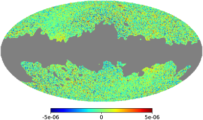
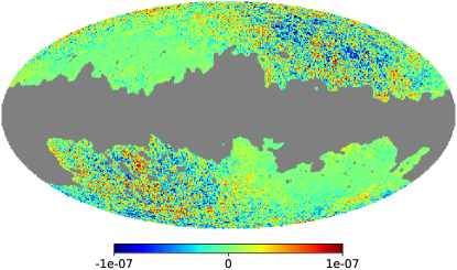
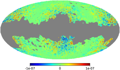
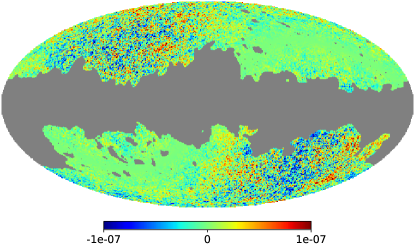
Figure 1: Map of the tSZ effect from the MILCA component-separation method in $y$-map units (top left) and the expected modulated CMB signal (top right) generated using the SMICA-NOSZ CMB map in units of $T_{0}$. The bottom left and right figures are the CMB anisotropies modulated in orthogonal directions to the CMB dipole, as explained in the text after Eq. (17). The greyed out region shows the mask used for our analysis. NILC and 2D-ILC $y$ maps, as well as 2D-ILC CMB modulated anisotropies, are not shown, since they look essentially the same as the maps presented here. Note that the map of the tSZ effect (top left) has a different scale bar when compared to the other three (i.e., the modulation signal is about 50 times weaker).

Equation (7) can thus be written as

$$\delta I^{\prime}(\mathbf{\hat{n}}^{\prime}) =If(x)\Bigl{(}1+\beta\mu Y(x)+3\beta\mu\Bigr{)}\times$$

$$\Bigl{(}\frac{\delta T(\mathbf{\hat{n}}^{\prime})}{T_{0}}+\beta\mu+y(\hat{\mathbf{n}}^{\prime})Y(x)-y(\hat{\mathbf{n}}^{\prime})\beta\mu x\frac{dY(x)}{dx}\Bigr{)}$$ (13)

or more explicitly, to first order in $\beta$,

$$\frac{\delta I^{\prime}(\mathbf{\hat{n}}^{\prime})}{If(x)}=\thinspace \frac{\delta T(\mathbf{\hat{n}}^{\prime})}{T_{0}}+\beta\mu\left[1+3\frac{\delta T(\mathbf{\hat{n}}^{\prime})}{T_{0}}\right]$$

$$+Y(x)\left[y(\mathbf{\hat{n}}^{\prime})+\beta\mu\frac{\delta T(\mathbf{\hat{n}}^{\prime})}{T_{0}}\right]$$

$$+\beta\mu y(\mathbf{\hat{n}}^{\prime})\left[3Y(x)+Y^{2}(x)-x\frac{dY(x)}{dx}\right],$$ (14)

where we have split up each line on the right-hand side according to the frequency dependence. Assuming perfect component separation, and comparing with Eq. (5), the first line of Eq. (14) shows that the boost induces a pure dipole ($\beta\mu$), an aberration effect ($\delta T(\mathbf{\hat{n}}^{\prime})/T_{0}-\delta T(\mathbf{\hat{n}})/T_{0}$), and a dipolar modulation ($3\beta\mu\delta T/T_{0}$) of the CMB. The first effect is the classical CMB dipole, which has been measured many times most recently by Planck (Planck Collaboration I 2019), with the highest accuracy so far achieved. The effects of aberration and dipolar modulation (both frequency-independent and frequency-dependent parts) were measured in Planck Collaboration XXVII (2014) at a combined significance level of $5\thinspace\sigma$.

In the second line of Eq. (14) we see that the boost also induces a change in a map of the tSZ effect. The original $y$ signal is aberrated ($y(\mathbf{\hat{n}}^{\prime})-y(\mathbf{\hat{n}})$) and also gains a contribution from the dipolar modulated CMB ($\beta\mu\delta T/T_{0}$). This last effect is what we measure in this paper for the first time. Its expected signal can be seen in Fig. 1 (top right panel), along with the full $y$ map obtained via the MILCA method (Hurier et al. 2013, Fig. 1 top left). It is worth noting that although the contribution to the tSZ map is a dipolar modulation of the CMB anisotropies, this induces power in the $y$ map that is modulated like a quadrupolar pattern (due to the lack of correlation between the CMB anisotropies and $y$ signal). That is, a $y$ map contains more power in the poles of the dipole, relative to the corresponding equator (see Fig. 1). It should be possible to pull out this signal compared with modulation patterns oriented in orthogonal directions (lower panels of Fig. 1).

We note that the final line in Eq. (14) is simply the dipole modulation of the tSZ effect, with a peculiar frequency dependence (Chluba et al. 2005). In principle one could generate a map of the anisotropies in this new frequency dependence and use the known CMB dipole to measure the $y$ anisotropies again. Such a measurement would be correlated with the original $y$ map, but would have independent noise properties and also have a very low amplitude. From a practical perspective it is unlikely that such a measurement would yield any significant information increase, since the signal is contaminated with relativistic tSZ and kSZ effects, and is suppressed by a factor of $\beta$ (Chluba et al. 2005).

3 Data

We look for the signal by cross-correlating a template map derived from the CMB temperature data with a $y$ map. Therefore it is important that the CMB map is free of $y$ residuals and that the $y$ map is free of CMB residuals, in order to avoid spurious correlations.

To this end, we use the so-called 2D-ILC CMB temperature map (first used for kSZ detection in Planck Collaboration Int. XIII 2014), which was produced by the “Constrained ILC” component-separation method designed by Remazeilles et al. (2011) to explicitly null out the contribution from the $y$-type spectral distortions in the CMB map. We also use the SMICA-NOSZ temperature map, similarly produced with express intent of removing the $y$-type spectral distortions, and which was generated with the Planck 2018 data release (Planck Collaboration IV 2019). Likewise, we use the corresponding 2D-ILC $y$ map, and the Planck MILCA $y$ map, which explicitly null out the contributions from a (differential) blackbody spectral distribution in the $y$ map (Hurier et al. 2013; Planck Collaboration XXII 2016). We also consider the Planck NILC $y$ map, which does not explicitly null out the blackbody contribution. The extra constraint to remove CMB anisotropies in the 2D-ILC $y$ map, or in the MILCA $y$ map, is at the expense of leaving more contamination by diffuse foregrounds and noise. In Planck Collaboration XXII (2016), the Planck NILC $y$ map was preferred over the 2D-ILC $y$ map to measure the angular power spectrum of tSZ anisotropies, the CMB contaminant being negligible compared to diffuse foregrounds. Conversely, to measure the dipole modulation of the CMB anisotropies in the $y$ map, the 2D-ILC and MILCA $y$ maps are preferred over the Planck NILC $y$ map because the latter does not fully null out the contribution from the CMB. This significantly contaminates the signal we are looking for, as can be seen in Appendix B. It is noted in Planck Collaboration XXII (2016) that for $\ell>2000$ the signal is dominated by correlated noise, and so we use the same cut as used in their analysis of $\ell_{max}=1411$, this is further justified in Sect. 4.2.

Figure 1 shows the mask used in our analysis. This is the union of the Planck 2018 data release common temperature confidence mask (Planck Collaboration IV 2019), and the corresponding $y$-map foreground masks (Planck Collaboration XXII 2016). This was then extended by $1^{\circ}$ and apodized with a $200{{}^{\scriptstyle\prime}}$ Gaussian beam. To account for any masked sections lost during the smoothing, the original mask was then added back. Tests were also done using the $y$-map point-source mask, with negligible changes seen in the results, and was thus omitted from the final analysis. This procedure aims to allow for the maximum signal while minimizing the foreground contamination. Various combinations of mask sizes and apodizations were also tested and final results were consistent, independent of the choice of mask.

4 Analysis

From Eq. (14) we see that a map of the tSZ effect ($\mathcal{M_{\mathrm{SZ}}}$) contains the following terms (for each pixel, or direction $\mathbf{\hat{n}}$):

$$\mathcal{M_{\mathrm{SZ}}}=y+\eta^{y}+\beta\mu\frac{\delta T}{T_{0}},$$ (15)

where $\eta^{y}$ is simply the noise in the $y$ map, and we have neglected the aberration effect. Our goal is to isolate the final term in Eq. (15), which we do via a suitable cross-correlation with a CMB map. A map of the CMB ($\mathcal{M}_{\mathrm{CMB}}$) contains the following terms:

$$\mathcal{M_{\mathrm{CMB}}}=\frac{\delta T}{T_{0}}+\eta^{T}+3\beta\mu\frac{\delta T}{T_{0}},$$ (16)

where we have explicitly removed the full dipole term, and $\eta^{T}$ is the noise in the CMB map. If we multiply our CMB map (Eq. 16) with $\beta\mu$ and cross-correlate that with our tSZ map (Eq. 15), then we can directly probe the dipole modulation. This of course neglects the noise and modulation terms in the CMB map, which we are justified in doing because the noise term is sub-dominant, except at very small scales (we make the restriction $\ell_{\max}=1411$, so that the $y$ map and CMB maps are still signal dominated Planck Collaboration XXII 2016), and because the modulation term becomes second order in $\beta$. Equivalently one could directly cross-correlate Eq. (15) with Eq. (16) and look for the signal in harmonic space from the coupling of $\ell$ and $\ell\pm 1$ modes.

In Planck Collaboration XXVII (2014) a quadratic estimator was used to determine the dipole aberration and modulation, in essence using the auto-correlation of the CMB fluctuation temperature maps, weighted appropriately to extract the dipole signal. The auto-correlation naturally introduces a correlated noise term, which must be well understood for this method to work. In this paper we take advantage of the fact that we know the true CMB fluctuations with excellent precision and therefore the signal that should be present in the $y$ map. We can therefore exploit the full angular dependence of the modulation signal and remove much of the cosmic variance that would be present in the auto-correlation.

In order to implement this idea we define three templates, $B_{i}$ (with $i=1,2,3$) as

$$B_{i}(\hat{\mathbf{n}}) =\beta\hat{\mathbf{n}}\cdot\hat{\mathbf{m}}_{i}\frac{\delta T}{T_{0}}(\hat{\mathbf{n}}),$$ (17)

where $\beta=v/c$ is $1.23357\times 10^{-3}$ (Planck Collaboration I 2019) and $\hat{\mathbf{m}}_{1},\hat{\mathbf{m}}_{2},\hat{\mathbf{m}}_{3}$ are the CMB dipole direction, an orthogonal direction in the Galactic plane, and the third remaining orthogonal direction (see Fig. 1 and Planck Collaboration XXVII 2014, for a similar approach). Note that in Eq. (17), we simply use our CMB map in place of $\delta T/T_{0}$. We use two distinct methods to accomplish this, discussed in detail in Sects. 4.1 and 4.2.

In the region where the CMB is signal dominated we can regard $\delta T/T_{0}$ as fixed, and thus our templates $B_{i}$ are fixed. Due to the presence of the CMB dipole, the signal $B_{1}$ should be present in the $y$ map. We can therefore directly cross-correlate $B_{1}$ with our $y$ map (Eq. 15) to pull out the signal. Likewise, the cross-correlation of $B_{2}$ and $B_{3}$ with our $y$ map should give results consistent with noise, although the coupling with the noise and mask leads to a bias that is recovered through simulations.

Our $y$ simulations are generated by first computing the power spectra of our data $y$ maps; specifically we apply the MASTER method using the NaMASTER routine (Alonso et al. 2019) to account for the applied mask (Hivon et al. 2002). Then we generate $y$ maps using this power-spectrum with the HEALPix (Górski et al. 2005) routine synfast. This is done separately for the 2D-ILC and MILCA maps because they have different noise properties (and thus different total power spectra). For our simulations that include the dipolar modulated CMB anisotropies we add the last term of Eq. (15). We finally apply a Gaussian smoothing of 5^′ to model the telescope beam.

For each analysis method (to be described in the following subsections) we estimate the amplitude of the dipole ($\hat{\beta}_{i}$) in each of the three orthogonal directions. We apply the same analysis on a suite of 1000 $y$ simulations, generated with and without the dipolar modulation term in Eq. (15). We are then able to generate a covariance that appropriately contains the effects of the mask we use and are able to compute any bias that the mask induces. On the assumption (verified by our simulations) that the $\hat{\beta}_{i}$ estimators are Gaussian, we are able to compute a value of $\chi^{2}$ for the case of no CMB term and with the CMB term (see Table 1). We can then apply Bayes’ theorem along with our covariance to calculate the probability that each model is true (with or without the CMB term) and the posterior of our dipole parameters ($\beta,l,b$), summarized in Table 1 and Fig. 2.

We estimate the covariance $C_{ij}$ of the $\hat{\beta}_{i}$ using the simulations and calculate the $\chi^{2}$ as

$$\chi^{2}_{k} =\sum_{ij}\left(\hat{\beta}_{i}-\left<\hat{\beta}_{i}\right>_{k}\right)C^{-1}_{ij}\left(\hat{\beta}_{j}-\left<\hat{\beta}_{j}\right>_{k}\right),$$ (18)

where $k$ denotes whether the expectation value in the sum is taken over the simulations that do or do not include the CMB term. For definiteness we define the null hypothesis $H_{0}$ ($k=0$) to not include the CMB term, while hypothesis $H_{1}$ ($k=1$) does include the CMB term. We can then directly calculate the probability that $H_{k}$ is true given the data ($\hat{\beta}_{i}$) as

$$P(H_{k}|\hat{\beta}_{i}) =P(\hat{\beta}_{i}|H_{k})P(H_{k}),$$ (19)

$$P(\hat{\beta}_{i}|H_{k}) =\frac{1}{\sqrt{|2\pi C|}}e^{-\chi^{2}_{k}/2}.$$ (20)

We can calculate the odds ratio, $O_{10}$, on the assumption that the two hypotheses are equally likely,

$$O_{10} \equiv\frac{P(H_{1}|\hat{\beta}_{i})}{P(H_{0}|\hat{\beta}_{i})}=\frac{e^{-\chi^{2}_{1}/2}}{e^{-\chi^{2}_{0}/2}}.$$ (21)

This quantity tells us to what degree $H_{1}$ should be trusted over $H_{0}$. Assuming that the two hypotheses are exhaustive, it is directly related to the probability that the individual hypotheses are true:

$$P(H_{0}|\hat{\beta}_{i}) =\frac{1}{1+O_{10}},$$ (22)

$$P(H_{1}|\hat{\beta}_{i}) =\frac{O_{10}}{1+O_{10}}.$$ (23)

These quantities and the $\chi^{2}_{k}$ values are given in Table 1.

We can also generate a likelihood for our parameters with the same covariance matrix:

$$\mathcal{L}(\beta_{i}) =\frac{1}{\sqrt{|2\pi C|}}e^{-\chi^{2}/2},$$ (24)

where we define the modified $\chi^{2}$ as above. We can then apply Bayes’ theorem with uniform priors on the $\beta_{i}$, equating the posterior of $\beta_{i}$ with Eq. (24). A simple conversion allows us to obtain the posterior of the parameters in spherical coordinates $(\tilde{\beta},\tilde{l},\tilde{b})$. We show this in Fig. 2 for our two analyses, using the 2D-ILC and MILCA maps.

In the following subsections we describe two methods of cross-correlation: the first we perform directly in map-space; and the second is performed in harmonic space. An advantage of using two independent methods is that their noise properties are different; for example, working in harmonic space introduces complications with masking, whereas in map space, although it may not be clear how to optimally weight the data, the estimator has less sensitivity to large-scale systematic effects. Thus, the advantage of using two approaches will become apparent when we try to assess the level of systematic error in our analysis.

4.1 Map-space method

First we apply our mask to the templates $B_{i}$ and $y$ map. Then we locate all peaks (i.e., local maxima or minima) of the template map $B_{i}$ and select a patch of radius $2$ .${}^{\circ}0$ around each peak. Our specific implementation of the peak method follows earlier studies, for example Planck Collaboration VII (2019). The weighting scheme has not been shown to be optimal, but a similar approach was used for determining constraints on cosmic birefringence Contreras et al. (2017) and gave similar results to using the power spectra (and the issue of weighting is further discussed in Jow et al. 2019a). Intuitively we would expect that sharper peaks have a higher signal, and hence that influences our choice for the weighting scheme described below. For every peak we obtain an estimate of $\hat{\beta}_{i}$ by the simple operation

$$\hat{\beta}_{i,p} =\beta\frac{\sum_{k\in D(p)}B_{i,k}y_{k}}{\sum_{k\in D(p)}B_{i,k}^{2}},$$ (25)

where $D(p)$ is the collection of all unmasked pixels in a $2$ .${}^{\circ}0$ radius centred on pixel $p$, and $p$ is the position of a peak. Equation (25) is simply a cross-correlation in map space and by itself offers a highly-noisy (and largely unbiased) estimate.

We then combine all individual peak estimates with a set of weights ($w_{p}$) to give our full estimate:

$$\hat{\beta}_{i} =\frac{\sum_{p}w_{i,p}\hat{\beta}_{i,p}}{\sum_{p}w_{i,p}}.$$ (26)

The values of $w_{i,p}$ depend solely on the templates $B_{i}$, and they can be chosen to obtain the smallest uncertainties. We choose $w_{p}$ to be proportional to the square of the dipole, which ensures that peaks near the dipole direction (and anti-direction) are weighted more than those close to the corresponding equator. We further choose that the weights are proportional to the square of the Laplacian at the peak (Desjacques 2008); this favours sharply defined peaks over shallow ones. Finally we account for the scan strategy of the Planck mission by weighting by the 217-GHz hits map (Planck Collaboration VIII 2016, denoted $H^{217}_{p}$), though this choice provides no appreciable difference to our results. The weights then are explicitly

$$w_{i,p} =|\hat{\mathbf{n}}\cdot\hat{\mathbf{m}}_{i}|^{2}_{p}\left(\left.\nabla^{2}(B_{i})\right|_{p}\right)^{2}H^{217}_{p}.$$ (27)

We evaluate the Laplacian numerically in pixel space at pixel $p$. The weighting scheme closely resembles the bias factors that come about when relating peaks to temperature fluctuations (Bond & Efstathiou 1987), as used in Komatsu et al. (2011), Planck Collaboration Int. XLIX (2016) and Jow et al. (2019b).

Combining Eqs. (26) and (27) gives us our estimates, $\hat{\beta}_{i}$. We apply the method for each of our simulated $y$ maps, in exactly the same way as for the data.

4.2 Harmonic-space method

The alternative approach is to directly cross-correlate Eq. (17) with the $y$ map, and compare this to the auto-correlation of Eq. (17).

Our first step is identical to the previous method in that we mask the templates $B_{i}$ and $y$ maps. Under the assumption that the $y$ map contains the template ($B_{i}$), the $y$ multipoles are Gaussian random numbers with mean and variance given by

$$s^{i}_{\ell m} =\int d\Omega\thinspace\beta\thinspace\hat{\mathbf{m}}_{i}\cdot\hat{\mathbf{n}}\thinspace\frac{\delta T}{T_{0}}M(\Omega)Y^{*}_{\ell m},$$ (28)

$$\sigma^{2}_{\ell} =C^{y}_{\ell}+N^{y}_{\ell},$$ (29)

respectively, where $M(\Omega)$ is the mask over the sphere, $Y_{\ell m}$ are the spherical harmonics, and the $\hat{\mathbf{m}}_{i}$ are as defined in Eq. (17). Thus we can obtain an estimate of $\beta_{i}$ by taking the cross-correlation with inverse-variance weighting. We can demonstrate this simply by writing our $y$ map as a sum of our expected signal plus everything else,

$$y_{\ell m} =\frac{\beta_{i}}{\beta}s^{i}_{\ell m}+\eta^{y}_{\ell m}.$$ (30)

Here our signal is of course given when $\beta_{i}=\beta\delta_{1i}$ and all sources of noise, such as tSZ, are given by $\eta^{y}_{\ell m}$. We then cross-correlate with our template and sum over all multipoles with inverse-variance weighting. We explicitly consider noise in our template, that is our template ($\bar{s}^{i}_{\ell m}$) is related to Eq. (29) via, $\bar{s}^{i}_{\ell m}=s^{i}_{\ell m}+\eta^{t}_{\ell m}$, where $\eta^{t}_{\ell m}$ is the noise in our template. Then the cross-correlation looks like,

$$\sum_{\ell m}\bar{s}^{i^{\prime}}_{\ell m}y^{*}_{\ell m}/\sigma^{2}_{\ell} =\frac{\beta_{i}}{\beta}\sum_{\ell m}\bar{s}^{i^{\prime}}_{\ell m}(s^{i}_{\ell m})^{*}/\sigma^{2}_{\ell}$$

$$+\sum_{\ell m}\bar{s}^{i^{\prime}}_{\ell m}(\eta^{y}_{\ell m})^{*}/\sigma^{2}_{\ell},$$ (31)

and expanding it out, this becomes

$$\sum_{\ell m}s^{i^{\prime}}_{\ell m}y^{*}_{\ell m}/\sigma^{2}_{\ell}+\sum_{\ell m}\eta^{t}_{\ell m}y^{*}_{\ell m}/\sigma^{2}_{\ell} =\frac{\beta_{i}}{\beta}\sum_{\ell m}s^{i^{\prime}}_{\ell m}(s^{i}_{\ell m})^{*}/\sigma^{2}_{\ell}$$

$$+\frac{\beta_{i}}{\beta}\sum_{\ell m}\eta^{t}_{\ell m}(s^{i}_{\ell m})^{*}/\sigma^{2}_{\ell}$$

$$+\sum_{\ell m}s^{i^{\prime}}_{\ell m}(\eta^{y}_{\ell m})^{*}/\sigma^{2}_{\ell}$$

$$+\sum_{\ell m}\eta^{t}_{\ell m}(\eta^{y}_{\ell m})^{*}/\sigma^{2}_{\ell}.$$ (32)

The last term on the left and last three terms on the right are all statistically zero, since our template does not correlate with tSZ or any other types of noise and the noise in our template does not correlate with the template itself or with noise in the $y$ map (by assumption). Hence we can solve for $\beta_{i}$ neglecting those terms, to produce our estimator $\hat{\beta}_{i}$:

$$\hat{\beta}_{i} =\beta\sum_{i^{\prime}}\left[\sum_{\ell m}^{\ell_{\max}}s^{i}_{\ell m}(s^{i^{\prime}}_{\ell m})^{*}/\sigma^{2}_{\ell}\right]^{-1}\sum_{\ell m}^{\ell_{\max}}s^{i^{\prime}}_{\ell m}(y_{\ell m})^{*}/\sigma^{2}_{\ell}.$$ (33)

It is important to note that in practice we do not have $s^{i}_{\ell m}$, since we do not know the exact realization of noise in the CMB, so we instead use $\bar{s}^{i}_{\ell m}$. Using Weiner-filtered results would allow us to calculate $s^{i}_{\ell m}$, but adds complexity in the masking process. We can compare what the Weiner-filtered results would be,

$$\sum_{\ell}\frac{(C_{\ell}^{TT})^{2}}{C_{\ell}^{TT}+N_{\ell}^{TT}}\frac{(2\ell+1)}{\sigma_{\ell}^{2}},$$ (34)

to our results,

$$\sum_{\ell}(C_{\ell}^{TT}+N_{\ell}^{TT})\frac{(2\ell+1)}{\sigma_{\ell}^{2}}$$ (35)

and find the bias to be on the order of 2 % for $\ell_{\max}=1411$, justifying our use of the cut-off.

Equation (33) is in fact a direct solution for $\beta_{i}$ in the absence of noise, since it is the direct solution of Eq. (32) in the absence of noise.

Relating back to the map-space method, $s^{i}_{\ell m}$ are the spherical harmonic coefficients of the templates denoted previously by $B_{i}$, and $y_{\ell m}$ are the spherical harmonic coefficients of the $y$ map. The values for $s^{i}_{\ell m}(s^{i^{\prime}}_{\ell,m})^{*}$ and $s^{i}_{\ell m}(y_{\ell m})^{*}$ may be computed using the maps with the HEALPix (Górski et al. 2005) routine anafast. In the case of the term $s^{i}_{\ell m}(s^{i^{\prime}}_{\ell,m})^{*}$ this results in a $3\times 3$ matrix for each $\ell$, with the cross-power spectrum for the three templates on the off diagonals.

In the absence of a mask $M$ the signal $|s_{\ell m}|^{2}$ induces power in a $\cos^{2}{\theta}$ pattern. The presence of a mask (being largely quadrupolar in shape) induces power in a more complicated way, but has strong overlap with a $\cos^{2}{\theta}$ pattern as well. Therefore the application of a mask necessarily makes this method sub-optimal; however, since the template is masked in the same way, the method is unbiased.

We apply the method for each of our simulated $y$ maps, in exactly the same way as for the data, in order to assess whether the dipole modulation is detected.

5 Results

Table 1: Values of $\chi^{2}$ (with $N_{\rm dof}=3$) under the assumption of no dipolar modulation term (“No dipole”), and assuming the presence of the dipolar modulation term (“With dipole”) for the 2D-ILC CMB template map. We include the probability that hypotheses of “No dipole” and “With dipole” are true. All data and analysis combinations are consistent with the dipole modulation term. The deviations range from 6.2 to $6.6\thinspace\sigma$ for the harmonic-space analysis, and from 5.0 to $5.9\thinspace\sigma$ for the map-space analysis.

No dipole       With dipole Method $$\kern 4.00002pt\chi^{2} P(H_{0}|\hat{\beta}_{i}) \kern 4.00002pt\chi^{2} P(H_{1}|\hat{\beta}_{i}) 4.0\times 10^{-9\kern 4.00002pt} 1-4.0\times 10^{-9\kern 4.00002pt} 8.4\times 10^{-10} 1-8.4\times 10^{-10} 1.8\times 10^{-8\kern 4.00002pt} 1-1.8\times 10^{-8\kern 4.00002pt} 5.0\times 10^{-6} 1-5.0\times 10^{-6\kern 4.00002pt}$$                      Harmonic-space analysis 2D-ILC. 39.5              0.8        MILCA. 42.4              0.7        Map-space analysis 2D-ILC. 38.6              3.0        MILCA. 24.8              0.4       

Table 2: As in Table 1 but using SMICA-NOSZ CMB template maps.

No dipole       With dipole

Method $$\kern 4.00002pt\chi^{2}$$                     

Harmonic-space analysis

2D-ILC. 41.9              1.2       

MILCA. 45.4              1.6       

Map-space analysis

2D-ILC. 40.1              3.0       

MILCA. 27.9              0.4       

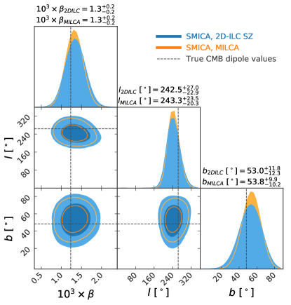
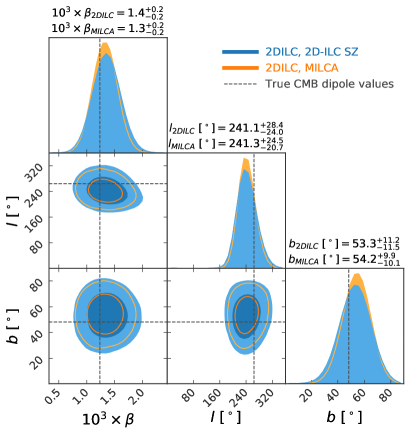
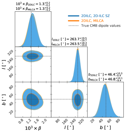
Figure 2: Posteriors for the CMB dipole parameters using the map-space analysis (top) and harmonic-space analysis (bottom). The left panels use the SMICA-NOSZ CMB maps, whereas the right use the 2D-ILC CMB maps. MILCA $y$ map results are shown in orange, and 2D-ILC $y$ map results are shown in blue. Black dashed lines show the best-fit parameters from direct measurements of the CMB dipole. Dark and light contours enclose 68 % and 95 %, respectively. Titles for each panel give the best-fit results, along with the 68 % uncertainties.

The main results of this paper are presented in Tables 1 and  2 and Fig. 2. They show how consistent the data are with the presence (or non-presence) of the dipole term, and the recovered posteriors of the dipole parameters, respectively. In the following subsections we describe our results for each method in more detail.

5.1 Map-space results

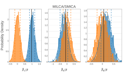
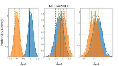
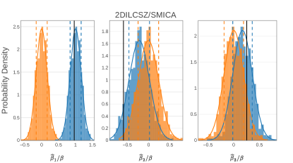
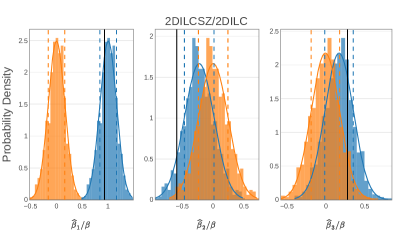
Figure 3: Histograms of $\hat{\beta}_{i}/\beta$ values (with 1, 2, and 3 corresponding to the CMB dipole direction, Galactic plane, and a third orthogonal direction) using the map-space analysis for MILCA (top) and 2D-ILC (bottom) $y$ maps, and for CMB template maps SMICA-NOSZ (left) and 2D-ILC (right). Blue histograms are simulations with the dipolar modulation term, and orange histograms are simulations without. Black vertical lines denote the values of the data, demonstrating that they are much more consistent with the existence of the dipolar modulation term than without it. Dashed lines show the 68 % regions for a Gaussian fit to the histograms.

First we compare the consistency of the data with our two sets of simulations (with and without the dipole term). This comparison shown in Fig. 3, with blue histograms being the simulations with the dipole term and orange histograms without. The data (black line) for 2D-ILC and MILCA can clearly be seen to be consistent with the simulations with the dipole term; this observation is made quantitative from examination of the $\chi^{2}$ (see Tables 1 and 2). The map-space method is more susceptible to biases induced by the mask, particularly in the off-dipole directions, $\hat{\beta_{2}}$ and $\hat{\beta_{3}}$; this is due to subtle correlations between the mask and templates, but has only a small effect in those directions (at the level of a few tenths of $\sigma$), as can be seen in Fig. 3. Converted into the equivalent probabilities for Gaussian statistics, we can say that the dipole modulation is detected at the 5.0 to $5.9\thinspace\sigma$ level.

5.2 Harmonic-space results

Figure 4 is the equivalent of Fig. 3, but for the harmonic-space analysis. Similar to the previous subsection the data are much more consistent with the modulated simulations than the unmodulated simulations. Tables 1 and  2 contain the explicit $\chi^{2}$ values and verify this quantitatively. The harmonic-space method is somewhat susceptible to biases induced by the mask, due to the complex coupling that occurs, mainly between the $\ell$ and $\ell\pm 2$ modes. This can be seen in the slight bias in the results for $\hat{\beta}_{2}$ and $\hat{\beta}_{3}$. Nevertheless, we can say that we confidently detect the dipole modulation at the 6.2 to $6.6\thinspace\sigma$ level.

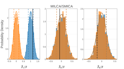
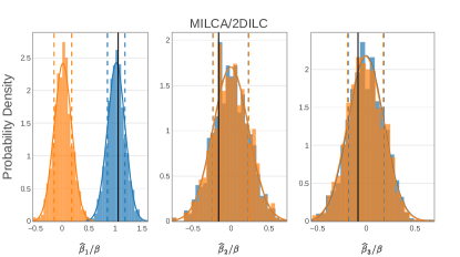
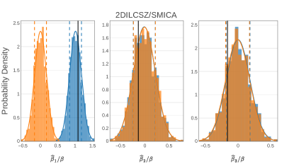
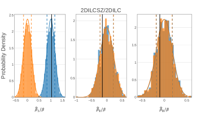
Figure 4: As in Fig. 3, except now for the harmonic-space analysis.

6 Systematics

We have generated results using two distinct methods, namely the map-space method and harmonic-space method, with two distinct CMB maps and two distinct $y$ maps, and have shown the results to be consistent with the presence of a dipole-modulation signal in the expected direction. Each test is subject to slightly different systematics, but since the results are consistent, we can conclude that there is likely no significant systematic interfering with the results. Further tests, relaxing the limits of $\ell_{\rm max}=1411$ show that it is possible to achieve even higher levels of significance using smaller-scale data (see Appendix C). In that sense, the results in this paper are conservative; however, if it becomes possible to construct reliable $y$ maps out to higher multipoles then it should be possible to achieve a detection of the dipole modulation at perhaps twice the number of $\sigma$ as found here.

6.1 Residuals in the component separation

The NILC $y$ maps are known to contain some remnant CMB contamination, unlike the MILCA and 2D-ILC $y$ maps, which have been generated with the express purpose of eliminating the CMB contribution. This contaminates the signal we are looking for; the results from the NILC $y$ maps may be seen in Appendix B. Any contamination remaining in the MILCA and 2D-ILC $y$ maps is sufficiently low that is does not hide the dipole modulation signal.

6.2 Galactic foregrounds

It is known that the $y$ maps are contaminated by Galactic foregrounds; however, as the results here are from a cross-correlation of the modulated CMB maps with the $y$ maps such contamination does not have a large effect on the results. To further support this, a number of different mask sizes and combinations were tested, with the final mask selected because among those choices consistent with the more conservative masks, it gave the highest signal-to-noise ratio. Larger masks serve only to decrease the signal-to-noise of the data. This suggests that foregrounds have only a small effect on the detection of the dipole modulation. Foregrounds have been mentioned as a potential issue in previous results (Planck Collaboration XXII 2016).

7 Conclusions

Due to the existence of the CMB dipole, a tSZ map necessarily contains a contaminating signal that is simply the dipole modulation of the CMB anisotropies. This occurs because CMB experiments do not directly measure temperature anisotropies, but instead measure intensity variations that are conventionally converted to temperature variations. This contamination adds power to the tSZ map in a $Y_{20}$ pattern, with its axis parallel to the dipole direction. We have measured this effect and determined a statistically independent value of the CMB dipole, which is consistent with direct measurements of the dipole. Using a conservative multipole cut on the $y$ map, the significance of the detection of the dipole modulation signal is around 5 or $6\thinspace\sigma$, depending on the precise choice of data set and analysis method. This is a significant improvement from the 2 to $3\thinspace\sigma$ results in Planck Collaboration XXVII (2014). We also find that the contamination of the tSZ map contributes negligible noise to the bispectrum calculations (see Appendix A).

Appendix A The tSZ bispectrum

Fundamentally the modulation is a correlation between $C_{\ell}$ and $C_{\ell\pm 1}$. The signal considered here therefore shows up most prominently in the 4-point function (i.e., trispectrum) and thus we do not expect it to bias the measurements of the tSZ bispectrum; however, since the bispectrum is an important quantity for characterizing the tSZ signal, it is worth checking to ensure that the dipolar modulation does not add significant noise. In other words, we want to check if it is important to remove the dipole modulations before performing analysis of the tSZ bispectrum. Lacasa et al. (2012) and Bucher et al. (2010) describe in detail the calculation of the bispectrum and the binned bispectrum, and this is summarized below. The reduced bispectrum is given by

$$B_{\ell_{1}\ell_{2}\ell_{3}} =(N_{\ell_{1}\ell_{2}\ell_{3}})^{-1/2}$$

$$\times\sum_{m_{1}m_{2}m_{3}}\left(\begin{array}[]{ccc}\ell_{1}&\ell_{2}&\ell_{3}\\ m_{1}&m_{2}&m_{3}\end{array}\right)a_{\ell_{1}m_{1}}a_{\ell_{2}m_{2}}a_{\ell_{3}m_{3}},$$ (38)

where $\left(\begin{array}[]{ccc}\ell_{1}&\ell_{2}&\ell_{3}\\ m_{1}&m_{2}&m_{3}\end{array}\right)$ represent the Wigner-3$j$ functions and

$$N_{\ell_{1}\ell_{2}\ell_{3}}=\frac{(2\ell_{1}+1)(2\ell_{2}+1)(2\ell_{3}+1)}{4\pi}\left(\begin{array}[]{ccc}\ell_{1}&\ell_{2}&\ell_{3}\\ 0&0&0\end{array}\right)^{2}.$$ (41)

The normalized bispectrum is non-zero for terms where $m_{1}+m_{2}+m_{3}=0$, $|\ell_{2}-\ell_{2}|\geq\ell_{3}\geq\ell_{1}+\ell_{2}$, and $\ell_{1}+\ell_{2}+\ell_{3}$ is even (this is due to the term before the sum with $m_{1},m_{2},m_{3}=0$). Typically, the binned bispectrum is analysed to reduce the number of terms calculated and saved, which constitutes only a small loss of information because the bispectrum is expected to vary slowly with $\ell$ (Lacasa et al. 2012). The data are binned by breaking down the interval from $\ell_{\rm min}$ to $\ell_{\rm max}$ into $i$ bins, denoted by $\Delta_{i}$. An average for the bispectrum of a particular bin can then be calculated using

$$B_{i_{1}i_{2}i_{3}} =\frac{1}{\Xi_{i_{1}i_{2}i_{3}}}\sum_{\ell_{1}\in\Delta_{1}}\sum_{\ell_{2}\in\Delta_{2}}\sum_{\ell_{3}\in\Delta_{3}}B_{\ell_{1}\ell_{2}\ell_{3}},$$ (42)

where $\Xi_{i_{1}i_{2}i_{3}}$ is the number of non-zero elements in the given bin. Both the bispectrum and the binned bispectrum may be calculated using an integral over the map space as well, rather than in harmonic space. This is achieved by first generating the binned scalemaps defined by

$$y_{\Delta_{i}}(\mathbf{\hat{n}})=\sum_{\ell\in\Delta_{i},m}y_{\ell m}Y_{\ell m}(\mathbf{\hat{n}}),$$ (43)

where the sum goes from $\ell_{min}$ to $\ell_{max}$ in the bin $\Delta_{i}$. We can then use

$$B_{i_{1}i_{2}i_{3}}=\frac{1}{N_{i_{1}i_{2}i_{3}}}\int\mathrm{d}^{2}\mathbf{\hat{n}}\thinspace y_{\Delta_{1}}(\mathbf{\hat{n}})\thinspace y_{\Delta_{2}}(\mathbf{\hat{n}})\thinspace y_{\Delta_{3}}(\mathbf{\hat{n}})$$ (44)

which gives the weighted average of the bispectrum within the bins (Lacasa et al. 2012).

In Figs. 5 and 6 we show a subset of the binned normalized bispectra for the $y$ maps, with and without the dipole modulation. For simplicity, since we are just comparing the results of two simulated maps, there are no non-Gaussianities and no mask applied. This analysis was performed using the MILCA $y$ map and the SMICA-NOSZ CMB temperature map. Plots are constructed in the style suggested by Lacasa et al. (2012) for an $\ell_{\rm max}$ of 500 (and an $N_{\mathrm{side}}$ of 512 to speed up computation).

Useful definitions here are

$$\sigma_{1} =\ell_{1}+\ell_{2}+\ell_{3},$$ (45)

$$\sigma_{2} =\ell_{1}\ell_{2}+\ell_{1}\ell_{3}+\ell_{2}\ell_{3},$$ (46)

$$\sigma_{3} =\ell_{1}\ell_{2}\ell_{3},$$ (47)

$$\tilde{\sigma}_{2} =12\sigma_{2}/\sigma_{1}^{2}-3,\ \in[0,1],$$ (48)

$$\tilde{\sigma_{3}} =27\sigma_{3}/\sigma_{1}^{3},\ \in[0,1],$$ (49)

$$F =32(\tilde{\sigma_{2}}-\tilde{\sigma_{3}})/3+1,$$ (50)

$$S =\tilde{\sigma_{3}},$$ (51)

$$P =\sigma_{1},$$ (52)

where $P$ is the perimeter, each plot represents the results of a particular perimeter size, $F$ is plotted along the $y$-axis of the panels and $S$ is plotted along the $x$-axis of the panels.

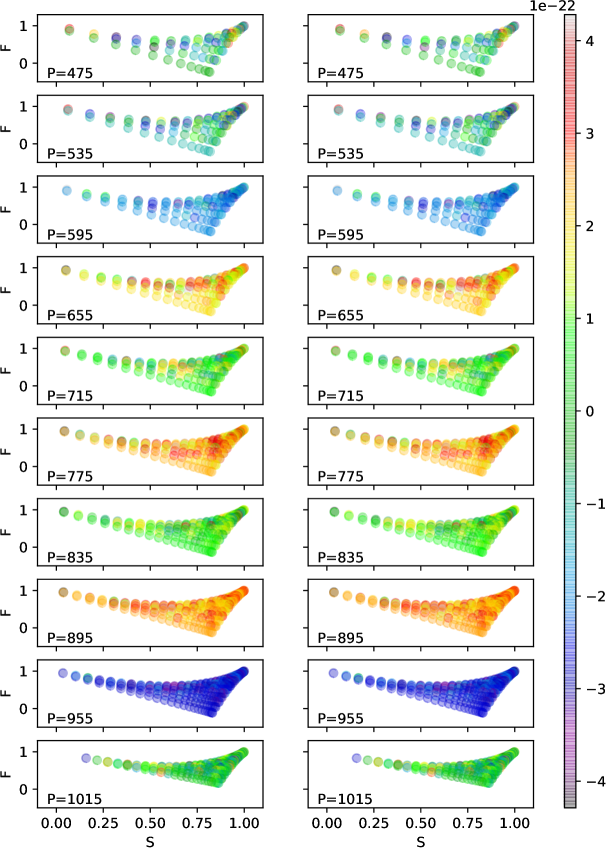
Figure 5: Binned bispectrum, for simulated $y$ maps, with $\ell_{\rm max}=500$ and bin sizes of 10, and “scalemaps” defined in Eq. 43, of $N_{\rm side}=512$. The left panels show the bispectrum for a simulated $y$ map with the dipole modulation and the right panels show the same with no dipole-modulation. The quantities $P$, $F$, and $S$ are as defined in Eqs. (52).

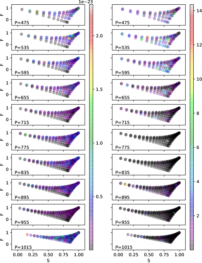
Figure 6: Absolute (left) and relative (right) difference between the bispectrum with and without the dipole-modulation term.

Our main goal is to determine whether the dipole modulation contamination of the $y$ maps is significant, and to what degree it is significant for current and future analysis as data improves. For this purpose a subset of the tested perimeter values are plotted, for data with the dipole modulation and without, and the absolute value of the differences. It does not appear that the dipole modulation has a noticeable effect on the bispectrum results.

Appendix B NILC y-map results

In creating the Planck $y$ maps using NILC, the choices were optimized for removal of the contamination by CMB, foregrounds, and noise. With the MILCA $y$ maps there was an additional constraint added to fully eliminate the CMB, at the expense of adding more foregrounds and noise contamination. For this reason the CMB contamination in the NILC $y$ maps is too high for us to robustly detect the dipole modulation. The 2D-ILC$y$ map was also produced with the express intent of removing all CMB contamination, and both it and the MILCA maps clearly show that the dipole modulation is present. For completeness, here we present the effect of the contamination in the NILC $y$ maps in Fig. 7. The dipole modulation signal is seen to be completely hidden by the CMB contamination.

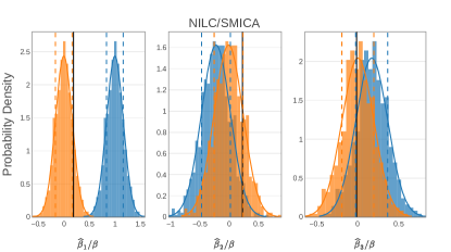
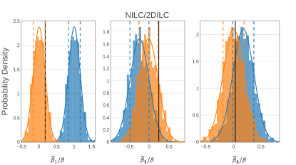
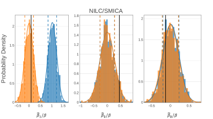
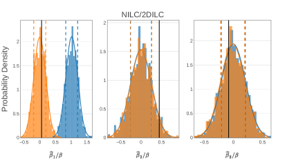
Figure 7: As in Figs. 3 (top) and 4 (bottom), except using the NILC $y$ maps. The top panels in this case show the results from the map-space method, while the bottom panels show those from the harmonic-space method.

Appendix C Increased $\ell$_max results

In our analysis for the harmonic-space method the results were truncated at $\ell_{\rm max}=1411$, since this is the recommendation from Planck Collaboration XXII (2016) to avoid the correlated noise and foreground contaminations present in higher $\ell$. If we were to assume that the simulations model the data properly up to a higher $\ell_{\rm max}$, and that we also trust the data up to this higher $\ell_{\rm max}$, then we would be able to achieve a greater significance than reported in the conclusions. This can be seen in the simulation results using the MILCA $y$ map and the SMICA-NOSZ CMB templates. These particular results are from 500 simulations for $N_{\rm side}=1024$, and $\ell_{\rm max}=2750$. The significance appears to be at the ${>}\thinspace 12\thinspace\sigma$ level. To do the analysis fully at this $\ell_{\rm max}$ the Weiner filter would also need to be applied to the CMB maps, as without it the bias would be much larger than the 2 % found in our analysis.

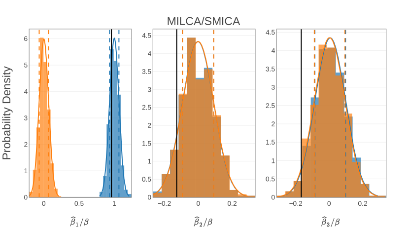
Figure 8: As in Fig. 4, but with $\ell_{\rm max}=2750$ compared to $\ell_{\rm max}=1411$ used in the paper. If we were to trust the $y$ map out to these multipoles, then these results would have a significance of ${>}\thinspace 12\thinspace\sigma$.

References

- Alonso et al. (2019) Alonso, D., Sanchez, J., Slosar, A., & Collaboration, L. D. E. S., A unified pseudo-C framework. 2019, Monthly Notices of the Royal Astronomical Society, 484, 4127, http://oup.prod.sis.lan/mnras/article-pdf/484/3/4127/27747342/stz093.pdf
- Bhattacharya et al. (2012) Bhattacharya, S., Nagai, D., Shaw, L., Crawford, T., & Holder, G. P., Bispectrum of the Sunyaev-Zel’dovich Effect. 2012, ApJ, 760, 5, 1203.6368
- Bond & Efstathiou (1987) Bond, J. R. & Efstathiou, G., The statistics of cosmic background radiation fluctuations. 1987, MNRAS, 226, 655
- Bucher et al. (2010) Bucher, M., van Tent, B., & Carvalho, C. S., Detecting bispectral acoustic oscillations from inflation using a new flexible estimator. 2010, Monthly Notices of the Royal Astronomical Society, 407, 2193, http://oup.prod.sis.lan/mnras/article-pdf/407/4/2193/3195988/mnras0407-2193.pdf
- Burles & Rappaport (2006) Burles, S. & Rappaport, S., Detecting the Aberration of the Cosmic Microwave Background. 2006, ApJ, 641, L1, astro-ph/0601559
- Challinor & van Leeuwen (2002) Challinor, A. & van Leeuwen, F., Peculiar velocity effects in high-resolution microwave background experiments. 2002, Phys. Rev. D, 65, 103001, astro-ph/0112457
- Chluba et al. (2005) Chluba, J., Hütsi, G., & Sunyaev, R. A., Clusters of galaxies in the microwave band: Influence of the motion of the Solar System. 2005, A&A, 434, 811, astro-ph/0409058
- Contreras et al. (2017) Contreras, D., Boubel, P., & Scott, D., Constraints on direction-dependent cosmic birefringence from Planck polarization data. 2017, J. Cosmology Astropart. Phys., 2017, 046, 1705.06387
- Desjacques (2008) Desjacques, V., Baryon acoustic signature in the clustering of density maxima. 2008, Phys. Rev. D, 78, 103503, 0806.0007
- Fixsen et al. (1996) Fixsen, D. J., Cheng, E. S., Gales, J. M., et al., The Cosmic Microwave Background Spectrum from the Full COBE FIRAS Data Set. 1996, ApJ, 473, 576, astro-ph/9605054
- Górski et al. (2005) Górski, K. M., Hivon, E., Banday, A. J., et al., HEALPix: A Framework for High-Resolution Discretization and Fast Analysis of Data Distributed on the Sphere. 2005, ApJ, 622, 759, astro-ph/0409513
- Hinshaw et al. (2009) Hinshaw, G., Weiland, J. L., Hill, R. S., et al., Five-Year Wilkinson Microwave Anisotropy Probe (WMAP) Observations: Data Processing, Sky Maps, and Basic Results. 2009, ApJS, 180, 225, 0803.0732
- Hivon et al. (2002) Hivon, E., Górski, K. M., Netterfield, C. B., et al., MASTER of the Cosmic Microwave Background Anisotropy Power Spectrum: A Fast Method for Statistical Analysis of Large and Complex Cosmic Microwave Background Data Sets. 2002, ApJ, 567, 2, astro-ph/0105302
- Hurier et al. (2013) Hurier, G., Macías-Pérez, J. F., & Hildebrandt, S., MILCA, a modified internal linear combination algorithm to extract astrophysical emissions from multifrequency sky maps. 2013, A&A, 558, A118, 1007.1149
- Jow et al. (2019a) Jow, D. L., Contreras, D., Scott, D., & Bunn, E. F., Taller in the saddle: constraining CMB physics using saddle points. 2019a, J. Cosmology Astropart. Phys., 2019, 031, 1811.05629
- Jow et al. (2019b) Jow, D. L., Contreras, D., Scott, D., & Bunn, E. F., Taller in the saddle: constraining CMB physics using saddle points. 2019b, J. Cosmology Astropart. Phys., 2019, 031, 1811.05629
- Kamionkowski & Knox (2003) Kamionkowski, M. & Knox, L., Aspects of the cosmic microwave background dipole. 2003, Phys. Rev. D, 67, 063001, astro-ph/0210165
- Kogut et al. (1993) Kogut, A., Lineweaver, C., Smoot, G. F., et al., Dipole Anisotropy in the COBE Differential Microwave Radiometers First-Year Sky Maps. 1993, ApJ, 419, 1, astro-ph/9312056
- Komatsu et al. (2011) Komatsu, E., Smith, K. M., Dunkley, J., et al., Seven-year Wilkinson Microwave Anisotropy Probe (WMAP) Observations: Cosmological Interpretation. 2011, ApJS, 192, 18, 1001.4538
- Lacasa et al. (2012) Lacasa, F., Aghanim, N., Kunz, M., & Frommert, M., Characterization of the non-Gaussianity of radio and IR point sources at CMB frequencies. 2012, Monthly Notices of the Royal Astronomical Society, 421, 1982, http://oup.prod.sis.lan/mnras/article-pdf/421/3/1982/5835850/mnras0421-1982.pdf
- Notari & Quartin (2015) Notari, A. & Quartin, M., CMB all-scale blackbody distortions induced by linearizing temperature. 2015, ArXiv e-prints, 1510.08793
- Planck Collaboration XXI (2014) Planck Collaboration XXI, Planck 2013 results. XXI. Power spectrum and high-order statistics of the Planck all-sky Compton parameter map. 2014, A&A, 571, A21, 1303.5081
- Planck Collaboration XXVII (2014) Planck Collaboration XXVII, Planck 2013 results. XXVII. Doppler boosting of the CMB: Eppur si muove. 2014, A&A, 571, A27, 1303.5087
- Planck Collaboration VIII (2016) Planck Collaboration VIII, Planck 2015 results. VIII. High Frequency Instrument data processing: Calibration and maps. 2016, A&A, 594, A8, 1502.01587
- Planck Collaboration XXII (2016) Planck Collaboration XXII, Planck 2015 results. XXII. A map of the thermal Sunyaev-Zeldovich effect. 2016, A&A, 594, A22, 1502.01596
- Planck Collaboration I (2019) Planck Collaboration I, Planck 2018 results. I. Overview, and the cosmological legacy of Planck. 2019, A&A, submitted, 1807.06205
- Planck Collaboration II (2019) Planck Collaboration II, Planck 2018 results. II. Low Frequency Instrument data processing. 2019, A&A, in press, 1807.06206
- Planck Collaboration III (2019) Planck Collaboration III, Planck 2018 results. III. High Frequency Instrument data processing. 2019, A&A, in press, 1807.06207
- Planck Collaboration IV (2019) Planck Collaboration IV, Planck 2018 results. IV. Diffuse component separation. 2019, A&A, in press, 1807.06208
- Planck Collaboration VII (2019) Planck Collaboration VII, Planck 2018 results. VII. Isotropy and statistics. 2019, A&A, in press, 1906.02552
- Planck Collaboration Int. XIII (2014) Planck Collaboration Int. XIII, Planck intermediate results. XIII. Constraints on peculiar velocities. 2014, A&A, 561, A97, 1303.5090
- Planck Collaboration Int. XLIX (2016) Planck Collaboration Int. XLIX, Planck intermediate results. XLIX. Parity-violation constraints from polarization data. 2016, A&A, 596, A110, 1605.08633
- Remazeilles et al. (2011) Remazeilles, M., Delabrouille, J., & Cardoso, J.-F., CMB and SZ effect separation with constrained Internal Linear Combinations. 2011, MNRAS, 410, 2481, 1006.5599
- Rubiño-Martín & Sunyaev (2003) Rubiño-Martín, J. A. & Sunyaev, R. A., Discriminating between unresolved point sources and ‘negative’ Sunyaev-Zel’dovich clusters in cosmic microwave background maps. 2003, MNRAS, 344, 1155, astro-ph/0211430