Scaling and local limits of Baxter permutations through coalescent-walk processes

Abstract

Baxter permutations, plane bipolar orientations, and a specific family of walks in the non-negative quadrant are well-known to be related to each other through several bijections. We introduce a further new family of discrete objects, called coalescent-walk processes, that are fundamental for our results. We relate these new objects with the other previously mentioned families introducing some new bijections.

We prove joint Benjamini–Schramm convergence (both in the annealed and quenched sense) for uniform objects in the four families. Furthermore, we explicitly construct a new fractal random measure of the unit square, called the coalescent Baxter permuton and we show that it is the scaling limit (in the permuton sense) of uniform Baxter permutations.

To prove the latter result, we study the scaling limit of the associated random coalescent-walk processes. We show that they converge in law to a continuous random coalescent-walk process encoded by a perturbed version of the Tanaka stochastic differential equation. This result has connections (to be explored in future projects) with the results of Gwynne, Holden, Sun (2016) on scaling limits (in the Peanosphere topology) of plane bipolar triangulations.

We further prove some results that relate the limiting objects of the four families to each other, both in the local and scaling limit case.

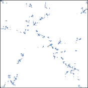
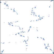
Figure 1: The diagrams of two uniform Baxter permutations of size 3253 (left) and 4520 (right). (How these permutations were obtained is discussed in Appendix C).

1 Introduction and main results

Baxter permutations were introduced by Glen Baxter in 1964 [3] to study fixed points of commuting functions. Baxter permutations are permutations avoiding the two vincular patterns $2\underbracket{41}3$ and $3\underbracket{14}2$, i.e. permutations $\sigma$ such that there are no indices $i<j<k$ such that $\sigma(j+1)<\sigma(i)<\sigma(k)<\sigma(j)$ or $\sigma(j)<\sigma(k)<\sigma(i)<\sigma(j+1)$.

In the last 30 years, several bijections between Baxter permutations, plane bipolar orientations and certain walks in the plane have been discovered. These relations between discrete objects of different nature are a beautiful piece of combinatorics that we aim at investigating from a more probabilistic point of view in this extended abstract. The goal of our work is to explore local and scaling limits of these objects and to study the relations between their limits. Indeed, since these objects are related by several bijections at the discrete level, we expect that most of the relations among them also hold in the “limiting discrete and continuous worlds”.

We mention that some limits of these objects (and related ones) were previously investigated. Dokos and Pak [11] explored the expected limit shape of doubly alternating Baxter permutations, i.e. Baxter permutations $\sigma$ such that $\sigma$ and $\sigma^{-1}$ are alternating. In their article they claimed that “it would be interesting to compute the limit shape of random Baxter permutations”. One of the main goals of our work is to answer this question by proving permuton convergence for uniform Baxter permutations (see Theorem 1.5 below). For plane walks (i.e. walks in $\mathbb{Z}^{2}$) conditioned to stay in a cone, we mention the remarkable works of Denisov and Wachtel [10] and Duraj and Wachtel [12] where they proved (together with many other results) convergence towards Brownian meanders or excursions in cones. This allowed Kenyon, Miller, Sheffield and Wilson [20] to show that the quadrant walks encoding uniformly random plane bipolar orientations (see Section 2.2 for more details) converge to a Brownian excursion of correlation $-1/2$ in the quarter-plane. This is interpreted as Peanosphere convergence of the maps decorated by the Peano curve (see Section 2.2 for further details) to a $\sqrt{4/3}$-Liouville Quantum Gravity (LQG) surface decorated by an independent $\text{SLE}_{12}$. This result was then significantly strengthened by Gwynne, Holden and Sun [14] who proved joint convergence for the map and its dual, in the setting of infinite-volume triangulations. In proving Theorem 1.5 we extend some of the methods and results of [14], with a key difference in the way limiting objects are defined. We discuss this in more precise terms at the end of this introduction.

So far we have considered three families of objects: Baxter permutations (denoted by $\mathcal{P}$); walks in the non-negative quadrant $(\mathcal{W})$ starting on the $y$-axis and ending on the $x$-axis, with some specific admissible increments defined in the forthcoming Equation 4; and plane bipolar orientations $(\mathcal{O})$. For our purposes, specifically for the proof of the permuton convergence, we introduce in Section 2.4 a fourth family of objects called coalescent-walk processes $(\mathcal{C})$.

We denote by $\mathcal{W}_{n}$ the subset of $\mathcal{W}$ consisting of quadrant walks of size $n$ (and similarly $\mathcal{C}_{n},\mathcal{P}_{n},\mathcal{O}_{n}$ for the other three families). We will present four size-preserving bijections (denoted using two letters that refer to the domain and co-domain) between these four families, summarized in the following diagram:

$$\leavevmode\hbox to72.64pt{\vbox to46.41pt{\text{[drawing]}}}\;, {\mathcal{W}} {\mathcal{C}} {\mathcal{O}} {\mathcal{P}} \scriptstyle{\operatorname{WC}} \scriptstyle{\operatorname{CP}} \scriptstyle{\operatorname{OW}} \scriptstyle{\operatorname{OP}} {\mathcal{W}} {\mathcal{C}} {\mathcal{O}} {\mathcal{P}} \scriptstyle{\operatorname{WC}} \scriptstyle{\operatorname{CP}} \scriptstyle{\operatorname{OW}} \scriptstyle{\operatorname{OP}}$$ (1)

where the mapping $\operatorname{OW}$ was introduced in [20] and $\operatorname{OP}$ in [5]; the others are new. Our first result is the following:

Theorem 1.1.

The diagram in Equation 1 commutes. In particular, $\operatorname{CP}\circ\operatorname{WC}:\mathcal{W}\to\mathcal{P}$ is a size-preserving bijection.

Our second result deals with local limits, more precisely Benjamini–Schramm limits. Informally, Benjamini–Schramm convergence for discrete objects looks at the convergence of the neighborhoods (of any fixed size) of a uniformly distinguished point of the object (called root). In order to properly define the Benjamini–Schramm convergence for the four families, we need to present the respective local topologies. We defer this task to the complete version of this abstract, here we just mention that the local topology for graphs (and so plane bipolar orientations) was introduced by Benjamini and Schramm [4] while the local topology for permutations was introduced by the first author [6]. Local topologies for plane walks and coalescent-walk processes can be defined in a similar way. We denote by $\widetilde{\mathfrak{W}}_{\bullet}$ the completion of the space of rooted walks $\bigsqcup_{n\geq 1}\mathcal{W}_{n}\times[n]$ with respect to the metric defining the local topology. The spaces $\widetilde{\mathfrak{C}}_{\bullet},\widetilde{\mathfrak{S}}_{\bullet},\widetilde{\mathfrak{m}}_{\bullet}$ are defined likewise from $\mathcal{C},\mathcal{P},\mathcal{O}$.

We define below the candidate limiting objects. As a matter of fact, a formal definition requires an extension of the mappings in Equation 1 to infinite-volume objects (for the mappings $\operatorname{WC}$ and $\operatorname{OW}^{-1}$ also an extension to walks that are not conditioned in the quadrant). We do not present all the details of such extensions, but they can be easily guessed from our description of the mappings $\operatorname{WC},\operatorname{OW},\operatorname{CP}$ and $\operatorname{OP}$ given in Section 2.

Let $\nu$ denote the probability distribution on $\mathbb{Z}^{2}$ given by:

$$\nu=\frac{1}{2}\delta_{(+1,-1)}+\sum_{i,j\geq 0}2^{-i-j-3}\delta_{(-i,j)},\quad\text{where $\delta$ denotes the Dirac measure},$$ (2)

and let $\bar{\bm{W}}=(\bar{\bm{X}},\bar{\bm{Y}})=(\bar{\bm{W}}_{t})_{t\in\mathbb{Z}}$ be a bidirectional random plane walk with step distribution $\nu$, with value $(0,0)$ at time 0. Let $\bar{\bm{Z}}=\operatorname{WC}(\bar{\bm{W}})$ be the corresponding infinite coalescent-walk process, $\bar{\bm{\sigma}}=\operatorname{CP}(\bar{\bm{Z}})$ the corresponding infinite permutation on $\mathbb{Z}$ (in this context, an infinite permutation is a total order of $\mathbb{Z}$), and $\bar{\bm{m}}=\operatorname{OW}^{-1}(\bar{\bm{W}})$ the corresponding infinite map.

Theorem 1.2.

For every $n\in\mathbb{Z}_{>0}$, let $\bm{W}_{n}$, $\bm{Z}_{n}$, $\bm{\sigma}_{n}$, and $\bm{m}_{n}$ denote uniform objects of size $n$ in $\mathcal{W}_{n}$, $\mathcal{C}_{n}$, $\mathcal{P}_{n}$, and $\mathcal{O}_{n}$ respectively, related by the bijections of Equation 1. For every $n\in\mathbb{Z}_{>0}$, let $\bm{i}_{n}$ be an independently chosen uniform index of $[n]$. Then we have joint convergence in distribution in the space $\widetilde{\mathfrak{W}}_{\bullet}\times\widetilde{\mathfrak{C}}_{\bullet}\times\widetilde{\mathfrak{S}}_{\bullet}\times\widetilde{\mathfrak{m}}_{\bullet}$:

$$((\bm{W}_{n},\bm{i}_{n}),(\bm{Z}_{n},\bm{i}_{n}),(\bm{\sigma}_{n},\bm{i}_{n}),(\bm{m}_{n},\bm{i}_{n}))\xrightarrow[n\to\infty]{d}(\bar{\bm{W}},\bar{\bm{Z}},\bar{\bm{\sigma}},\bar{\bm{m}}).$$

Remark 1.3.

We give a few comments on this result.

1. The mapping $\operatorname{OW}^{-1}$ naturally endows the map $\bm{m}_{n}$ with an edge labeling and the root $\bm{i}_{n}$ of $\bm{m}_{n}$ is chosen according to this labeling.

2. We can also prove a quenched version of the above result (of annealed type) for all the four objects (not presented in this extended abstract). It entails (see [6, Theorem 2.32]) that consecutive pattern densities of $\bm{\sigma}_{n}$ jointly converge in distribution.

3. The fact that the four convergences are joint follows from the fact that the extensions of the mappings in Equation 1 to infinite-volume objects are a.s. continuous.

4. The annealed Benjamini-Schramm convergence for bipolar orientations to the so-called Uniform Infinite Bipolar Map was already proved in [15, Prop. 3.10].

Our third (and main) result is a scaling limit result for Baxter permutations (see Figure 1 for some simulations), in the framework of permutons developed by [18]. A permuton $\mu$ is a Borel probability measure on the unit square $[0,1]^{2}$ with uniform marginals, that is $\mu([0,1]\times[a,b])=\mu([a,b]\times[0,1])=b-a,$ for all $0\leq a\leq b\leq 1$. Any permutation $\sigma$ of size $n\geq 1$ may be interpreted as the permuton $\mu_{\sigma}$ given by the sum of Lebesgue area measures

$$\mu_{\sigma}(A)=n\sum_{i=1}^{n}\operatorname{Leb}\big{(}[(i-1)/n,i/n]\times[(\sigma(i)-1)/n,\sigma(i)/n]\cap A\big{)},$$ (3)

for all Borel measurable sets $A$ of $[0,1]^{2}$. Let $\mathcal{M}$ be the set of permutons. As for general probability measure, we say that a sequence of (deterministic) permutons $(\mu_{n})_{n}$ converges weakly to $\mu$ (simply denoted $\mu_{n}\to\mu$) if $\int_{[0,1]^{2}}fd\mu_{n}\to\int_{[0,1]^{2}}fd\mu,$ for every (bounded and) continuous function $f:[0,1]^{2}\to\mathbb{R}$. With this topology, $\mathcal{M}$ is compact. Convergence for random permutations is defined as follows:

Definition 1.4.

We say that a random permutation $\bm{\sigma}_{n}$ converges in distribution to a random permuton $\bm{\mu}$ as $n\to\infty$ if the random permuton $\mu_{\bm{\sigma}_{n}}$ converges in distribution to $\bm{\mu}$ with respect to the weak topology.

Random permuton convergence entails joint convergence in distribution of all (classical) pattern densities (see [1, Theorem 2.5]). The study of permuton limits, as well as other scaling limits of permutations, is a rapidly developing field in discrete probability theory, see for instance [1, 2, 7, 8, 17, 19, 21, 22, 23]. Our main result is the following:

Theorem 1.5.

Let $\bm{\sigma}_{n}$ be a uniform Baxter permutation of size $n$. There exists a random permuton $\bm{\mu}_{B}$ such that $\mu_{\bm{\sigma}_{n}}\stackrel{{\scriptstyle d}}{{\longrightarrow}}\bm{\mu}_{B}.$

An explicit construction of the limiting permuton $\bm{\mu}_{B}$, called the coalescent Baxter permuton, is given in Section 3.2. The proof of Theorem 1.5 is based on a result on scaling limits of the coalescent-walk processes $\bm{Z}_{n}$, which appears to be of independent interest, and is discussed in Section 3.1. In particular, the convergence of uniform Baxter permutations is joint with that of the conditioned versions of $\bm{W}_{n}$ and $\bm{Z}_{n}$ presented in Theorem 3.7.

We finally discuss the relations with the work of Gwynne, Holden and Sun [14]. They show that for infinite-volume bipolar oriented triangulations, the explorations of the two tree/dual tree pairs of the map and its dual converge jointly. The limit is the pair of planar Brownian motions which encode the same $\sqrt{4/3}$-LQG surface decorated by both an $\text{SLE}_{12}$ curve and the “dual” $\text{SLE}_{12}$ curve, traveling in a direction perpendicular (in the sense of imaginary geometry) to the original curve. As shown below (Lemma 2.7), the bijection of [5] between plane bipolar orientations and Baxter permutations can be rewritten in terms of the interaction of these two tree/dual tree pairs, which explains the connection between our work and the one of [14].

We prove Theorem 1.5 by extending some of their constructions to finite-volume general maps, which allows us to provide an analog of their result (that are restricted to triangulations) for general plane bipolar orientations in finite volume, jointly with the convergences above. More precisely, the coalescent-walk process defined in Section 2.4.1 is an extension of the random walk $\mathcal{X}$ defined in [14, Section 2.1]. The fact that it encodes the spanning tree of the dual map (Proposition 2.14) is a version of [14, Lemma 2.1], albeit we present it differently. Our main technical ingredient is the convergence of the coalescent-walk process driven by a random plane walk of Theorem 3.5. It corresponds to [14, Theorem 4.1]. The way the limiting object (the right-hand side of Equation 10) is defined is however very different, and the proofs differ as a consequence. In our case, it comes from a stochastic differential equation (Equation 7), for which existence and uniqueness are known from the literature [9, 24]. In their case, it is built using imaginary geometry, and characterized by its excursion decomposition. These are nonetheless two descriptions of the same object, providing an SDE formulation of an intricate imaginary geometry coupling. We wish to explore consequences of this in further works.

Outline of the extended abstract. The remainder of the abstract is organized as follows. In Section 2 we present the objects and the mappings involved in the diagram in Equation 1. Moreover, we sketch the proof of Theorem 1.1. Section 3 is devoted to developing the theory for the proof of Theorem 1.5. In particular, in Section 3.1 we present the aforementioned results for scaling limits of coalescent-walk processes, and in Section 3.2 we give an explicit construction of the limiting permuton for Baxter permutations. Finally, in Appendix A we prove our main technical ingredient (Theorem 3.5), and in Appendix B we finish the proof of Theorem 1.5. Note that we leave the proof of Theorem 1.2 out of this abstract.

2 Bipolar orientations, walks in the non-negative quadrant, Baxter permutations and coalescent-walk processes

2.1 Plane bipolar orientations

We recall that a planar map is a connected graph embedded in the plane with no edge-crossings, considered up to continuous deformation. A map has vertices, edges, and faces, the latter being the connected components of the plane remaining after deleting the edges. The outer face is unbounded, the inner faces are bounded.

Definition 2.1.

A plane bipolar orientation (or simply bipolar orientation) is a planar map with oriented edges such that

• there are no oriented cycles;

• there is exactly one vertex with only outgoing edges (the source, denoted $s$), and exactly one vertex with only incoming edges (the sink, denoted $s^{\prime}$); all other vertices, called non-polar, have both types of edges;

• the source and the sink are both incident to the outer face.

The size of a bipolar orientation $m$ is its number of edges and will be denoted with $|m|$.

Every bipolar orientation can be plotted in the plane in such a way that every edge is oriented from bottom to top (as done for example in Figure 2).

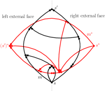
Figure 2: In black, a bipolar orientation $m$ of size 10. Note that every edge is oriented from bottom to top. In red, its dual map $m^{*}$. Similarly, we plot the dual map in such a way that every edge is oriented from right to left. This map will be used in several examples. In later pictures, the orientation of each edge is not displayed.

Given a bipolar orientation, an edge $e$ from $v$ to $w$ is bordered, in the clockwise cyclic order, by its bottom vertex, its left face, its top vertex, its right face. It is useful, for the consistency of definitions, to think of the external face as split in two (see Figure 2 for an example): the left external face, and the right external face.

There is a natural notion of duality for a bipolar orientation $m$. It is the classical duality for (unoriented) maps where the orientation of a dual edge between two primal faces is from right to left. The primal right external face becomes the dual source, and the primal left external face becomes the dual sink. This map $m^{*}$ is also a bipolar orientation (see Figure 2). The map $m^{**}$ is just the reversal of the map $m$: the source and sink are exchanged, and all edges are reversed.

Given a bipolar orientation $m$, its down-right tree $T(m)$ may be defined as a set of edges equipped with a parent relation, as follows.

• The edges of $T(m)$ are the edges of $m$.

• Let $e\in m$ and $v$ its bottom vertex.

  • If $v$ is the source, then $e$ has no parent edge in $T(m)$ (it is grafted to the root of $T(m)$);

  • if $v$ is not the source, the parent edge of $e$ in $T(m)$ is the right-most incoming edge of $v$.

The tree $T(m)$ can be drawn on top of $m$: the root of $T(m)$ corresponds to the source $s$ of $m$, internal vertices of $T(m)$ correspond to non-polar vertices of $m$, and leaves of $T(m)$ are the midpoints of some edges of $m$. Note that one can draw the trees $T(m)$ and $T(m^{**})$ on the map $m$ without any crossing (see the left-hand side of Figure 3 for an example).

We conclude this section recalling that the exploration of a tree $T$ is the visit of its vertices (or its edges) following the contour of the tree in the clockwise order.

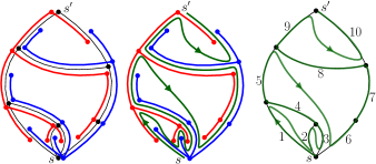
Figure 3: Left: A bipolar orientation $m$ with the trees $T(m)$ (in blue) and $T(m^{**})$ (in red). Middle: We add in green the interface path tracking the interface between the two trees (see Section 2.2). Right: We label the edges of the bipolar orientations following the interface path.

2.2 Kenyon-Miller-Sheffield-Wilson bijection

We now present a bijection between bipolar orientations and some walks in the non-negative quadrant $\mathbb{Z}_{\geq 0}^{2}$, introduced in [20, Section 2] by Kenyon, Miller, Sheffield and Wilson.

Let $m$ be a bipolar orientation. We consider the exploration of the tree $T(m)$ (highlighted in green in the middle picture of Figure 3) starting at the source $s$ and ending at the last visit of the sink $s^{\prime}$. Note that this path (when reversed) is also the exploration of the tree $T(m^{**})$ stopped at the last visit of the source $s$. This path, called interface path since it winds between the trees $T(m)$ and $T(m^{**})$, identifies an ordering on the set $E$ of edges of $m$ since every edge of $T(m)$ corresponds exactly to one edge of $m$ (see the right-hand side of Figure 3 for an example). Let $e_{1},e_{2},\dots,e_{|m|}$ be the edges of $m$ listed according to this order.

Definition 2.2.

Given a bipolar orientation $m$, the corresponding walk $\operatorname{OW}(m)=(W_{t})_{t\in[|m|]}=(X_{t},Y_{t})_{t\in[|m|]}$ of size $|m|$ in the non-negative quadrant $\mathbb{Z}_{\geq 0}^{2}$ is defined as follows: for $t\in[|m|]$, let $X_{t}$ be the distance in the tree $T(m)$ between the bottom vertex of $e_{t}$ and the root of $T(m)$ (corresponding to the source $s$), and let $Y_{t}$ be the distance in the tree $T(m^{**})$ between the top vertex of $e_{t}$ and the root of $T(m^{**})$ (corresponding to the sink $s^{\prime}$).

Remark 2.3.

The walk $(0,X_{1}+1,\ldots,X_{|m|}+1)$ is the height process of the tree $T(m)$. The walk $(0,Y_{|m|}+1,Y_{|m|-1}+1,\ldots,Y_{1}+1)$ is the height process of the tree $T(m^{**})$.

Suppose that the left external face has $h+1$ edges and the right external face has $k+1$ edges, for some $h,k\geq 0$. Then the walk $(W_{t})_{1\leq t\leq|m|}$ starts at $(0,h)$, ends at $(k,0)$, and stays in the non-negative quadrant $\mathbb{Z}_{\geq 0}^{2}$. We finally investigate the possible values for the increments of the walk, i.e. the values of $W_{t+1}-W_{t}$. We say that two edges of a tree are consecutive if one is the parent of the other. We first highlight that the interface path of the map $m$ has two different behaviors when following the edges $e_{t}$ and $e_{t+1}$:

• either it is following two consecutive edges of $T(m)$ (this is the case, for instance, of the edges $e_{3}$ and $e_{4}$ on the right-hand side of Figure 3);

• or it is first following $e_{t}$, then it is traversing a face of $m$, and finally is following $e_{t+1}$ (this is the case, for instance, of the edges $e_{5}$ and $e_{6}$ on the right-hand side of Figure 3).

When the latter case happens, the interface path splits the boundary of the traversed face in two parts, a left and a right boundary.

Therefore the increments of the walk are either $(+1,-1)$ (when $e_{t}$ and $e_{t+1}$ are consecutive) or $(-i,+j)$, for some $i,j\in\mathbb{Z}_{\geq 0}$ (when, between $e_{t}$ and $e_{t+1}$, the interface path is traversing a face with $i+1$ edges on the left boundary and $j+1$ edges on the right boundary). We denote by $A$ the set of possible increments, that is

$$A=\{(+1,-1)\}\cup\{(-i,j),i\in\mathbb{Z}_{\geq 0},j\in\mathbb{Z}_{\geq 0}\}.$$ (4)

We denote by $\mathcal{W}$ the set of walks in the non-negative quadrant, starting at $(0,h)$ and ending at $(k,0)$ for some $h\geq 0,k\geq 0$, with increments in $A$.

Theorem 2.4.

([20, Theorem 1]) The mapping $\operatorname{OW}:\mathcal{O}\to\mathcal{W}$ is a size-preserving bijection.

Example 2.5.

We consider the map $m$ in Figure 3. The corresponding walk $\operatorname{OW}(m)$ is:

$$\Big{(}(0,2),(0,3),(0,3),(1,2),(2,1),(0,3),(1,2),(2,1),(3,0),(2,0)\Big{)}.$$

2.3 Baxter permutations and bipolar orientations

In [5], a bijection between Baxter permutations and bipolar orientations is given. We give here a slightly different formulation of this bijection (more convenient for our purposes) and then in Lemma 2.7 we state that the two formulations are equivalent.

Definition 2.6.

Let $m$ be a bipolar orientation of size $n\geq 1$. Recall that to every edge of the map $m$ corresponds its dual edge in the dual map $m^{*}$. The Baxter permutation $\operatorname{OP}(m)$ associated with $m$ is the only permutation $\pi$ such that for every $1\leq i\leq n$, the $i$-th edge visited in the exploration of $T(m)$ corresponds to the $\pi(i)$-th edge visited in the exploration of $T(m^{*})$. We say that this edge corresponds to the index $i$.

An example is given in Figure 4. The following result proves that $\operatorname{OP}$ is a bijection.

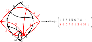
Figure 4: Left: The bipolar orientation $m$ and its dual $m^{*}$, already considered in Figure 2. We plot in black the labeling of the edges of $m$ obtained in Figure 3 and in red the labeling of the edges of $m^{*}$ obtained using the same procedure used for $m$. Right: The permutation $\operatorname{OP}(m)$ obtained by pairing the labels of the corresponding primal and dual edges between $m$ and $m^{*}$.

Lemma 2.7.

The function $\operatorname{OP}:\mathcal{O}\to\mathcal{P}$ is equal to the function $\Psi:\mathcal{O}\to\mathcal{P}$ defined in [5, Section 3.2]. Therefore $\operatorname{OP}$ is a size-preserving bijection.

The definition of $\Psi$ is the same as that of $\operatorname{OP}$, with $T(m^{*})$ replaced by $T(m^{-1})$, $m^{-1}$ denoting the symmetry of $m$ along the vertical axis. So the proof (that we omit) amounts to showing that these two trees visit the edges of $m$ in the same order.

2.4 Discrete coalescent-walk processes

Since the key ingredient for permuton convergence is the extraction of patterns (see Proposition B.1), we introduce in this section a new tool in order to “extract patterns from the plane walk” that encodes a Baxter permutation, namely coalescent-walk processes. Then, in Section 2.4.1, we present a bijection between walks in the non-negative quadrant and a specific kind of coalescent-walk processes, and in Section 2.4.2, we introduce a bijection between these coalescent-walk processes and Baxter permutations. Composing these two mappings we obtain another bijection between walks in the non-negative quadrant and Baxter permutations. Finally, in Section 2.5 we complete the proof of Theorem 1.1.

Definition 2.8.

Let $I$ be a (finite or infinite) interval of $\mathbb{Z}$. We call coalescent-walk process over $I$ a family $\{(Z^{(t)}_{s})_{s\geq t,s\in I}\}_{t\in I}$ of one-dimensional walks such that

• the walk $Z^{(t)}$ starts at zero at time $t$, i.e. $Z^{(t)}_{t}=0$;

• if $Z^{(t)}_{k}\geq Z^{(t^{\prime})}_{k}$ (resp. $Z^{(t)}_{k}\leq Z^{(t^{\prime})}_{k}$) at some time $k,$ then $Z^{(t)}_{k^{\prime}}\geq Z^{(t^{\prime})}_{k^{\prime}}$ (resp. $Z^{(t)}_{k^{\prime}}\leq Z^{(t^{\prime})}_{k^{\prime}}$) for every $k^{\prime}\geq k$.

Note that, as a consequence, if $Z^{(t)}_{k}=Z^{(t^{\prime})}_{k}$, at time $k,$ then $Z^{(t)}_{k^{\prime}}=Z^{(t^{\prime})}_{k^{\prime}}$ for every $k^{\prime}\geq k$. In this case, we say that $Z^{(t)}$ and $Z^{(t^{\prime})}$ are coalescing and call coalescent point of $Z^{(t)}$ and $Z^{(t^{\prime})}$ the point $(\ell,Z^{(t)}_{\ell})$ such that $\ell=\min\{k\geq\max\{t,t^{\prime}\}|Z^{(t)}_{k}=Z^{(t^{\prime})}_{k}\}$. We denote by $\mathfrak{C}(I)$ the set of coalescent-walk processes over some interval $I$.

2.4.1 The coalescent-walk process corresponding to a plane walk

We now introduce a particular family of coalescent-walk processes of interest for us. Let $I$ be a (finite or infinite) interval of $\mathbb{Z}$. Recall the definition of $A$ from Equation 4 page 4, and let $\mathfrak{W}_{A}(I)$ be the set of plane walks of time space $I$ (functions $I\to\mathbb{Z}^{2}$) with increments in $A$.

Take $W\in\mathfrak{W}_{A}(I)$ and denote $W_{t}=(X_{t},Y_{t})$ for $t\in I$. From $X$ and $Y$ we construct the family of walks $\{Z^{(t)}\}_{t\in I}$, called the coalescent-walk process associated with $W,$ by

• for $t\in I$, $Z^{(t)}_{t}=0;$

• for $t\in I$ and $k\in I\cap[t+1,+\infty),$

  $$Z^{(t)}_{k}=\begin{cases}Z^{(t)}_{k-1}+(Y_{k}-Y_{k-1}),&\quad\text{if}\quad Z^{(t)}_{k-1}\geq 0,\\ Z^{(t)}_{k-1}-(X_{k}-X_{k-1}),&\quad\text{if}\quad Z^{(t)}_{k-1}<0\text{ and }Z^{(t)}_{k-1}-(X_{k}-X_{k-1})<0,\\ Y_{k}-Y_{k-1},&\quad\text{if}\quad Z^{(t)}_{k-1}<0\text{ and }Z^{(t)}_{k-1}-(X_{k}-X_{k-1})\geq 0.\end{cases}$$ (5)

Let $\operatorname{WC}:\mathfrak{W}_{A}(I)\to\mathfrak{C}(I)$ map each $W\in\mathfrak{W}_{A}(I)$ to the corresponding coalescent-walk process, i.e. $\operatorname{WC}(W)=\{Z^{(t)}\}_{t\in I}$. We also set $\mathcal{C}_{n}=\operatorname{WC}(\mathcal{W}_{n})\subset\mathfrak{C}([n])$ and $\mathcal{C}=\cup_{n\in\mathbb{Z}_{\geq 0}}\mathcal{C}_{n}.$

We give a heuristic explanation of this construction in the following example.

Example 2.9.

We consider the plane walk $W=(W_{t})_{t\in[10]}$ starting at $(0,0)$ on the left-hand side of Figure 5. We plot in the second diagram of Figure 5 the walks $Y$ in red and $-X$ in blue. We now explain how we reconstruct the ten walks $\{Z^{(t)}\}_{1\leq t\leq 10}$ (in green on the right-hand side of Figure 5). The walk $Z^{(t)}$ starts at height zero at time $t$. Then,

• If $Z^{(t)}_{k-1}$ is non-negative (in particular at the starting point), then the increment $Z^{(t)}_{k}-Z^{(t)}_{k-1}$ is the same as the one of the red walk.

• If $Z^{(t)}_{k-1}$ is negative, then the increment $Z^{(t)}_{k}-Z^{(t)}_{k-1}$ is the same as the one of the blue walk, as long as this increment keeps $Z^{(t)}_{k}$ negative.

• Now if at time $k-1,$ $Z^{(t)}_{k-1}$ is negative but the blue increment would “force” it to cross (or touch) the $x$-axis (that is if $X_{k}-X_{k-1}\leq Z^{(t)}_{k-1}<0$), then $Z^{(t)}_{k}$ is equal to $Y_{k}-Y_{k-1}$ (i.e. $Z^{(t)}$ coalesces with $Z^{(k-1)}$ at time $k$). For instance this is the case of the second increment of the walk $Z^{(7)}$.

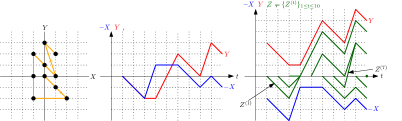
Figure 5: Left: A plane walk $(X,Y)$ starting at (0,0). Middle: The diagram of the walks $Y$ (in red) and $-X$ (in blue). Right: The two walks are shifted (one towards the top and one to the bottom) and the ten walks of the coalescent-walk process are plotted in green.

Observation 2.10.

The $y$-coordinates of the coalescent points of a coalescent-walk process in $\mathcal{C}(I)$ are non-negative.

2.4.2 The permutation associated with a coalescent-walk process

Given a coalescent-walk process $Z=\{Z^{(t)}\}_{t\in I}$ defined on a (finite or infinite) interval $I$, the relation $\leq_{Z}$ on $I$ defined as follows is a total order (we skip the proof of this fact):

$$i\leq_{Z}j\quad\iff\quad\{i<j\text{ and }Z^{(i)}_{j}<0\}\quad\text{or}\quad\{j<i\text{ and }Z^{(j)}_{i}\geq 0\}\quad\text{or}\quad\{i=j\}.$$ (6)

This definition allows to associate a permutation to a coalescent-walk process.

Definition 2.11.

Fix $n\in\mathbb{Z}_{\geq 0}$. Let $Z=\{Z^{(t)}\}_{t\in[n]}\in\mathcal{C}_{n}$ be a coalescent-walk process over $[n]$. Denote $\operatorname{CP}(Z)$ the permutation $\sigma\in\mathfrak{S}_{n}$ such that for $1\leq i,j\leq n$, $\sigma(i)\leq\sigma(j)\iff i\leq_{Z}j$.

We have that pattern extraction in the permutation $\operatorname{CP}(Z)$ depends only on a finite number of trajectories, a key step towards proving permuton convergence.

Proposition 2.12.

Let $\sigma$ be a permutation obtained from a coalescent-walk process $Z=\{Z^{(t)}\}_{t\in[n]}$ via the map $\operatorname{CP}$. Let $I=\{i_{1}<\dots<i_{k}\}\subset[n]$. Then $\operatorname{pat}_{I}(\sigma)=\pi$ if the following condition holds: for all $1\leq\ell<s\leq k,$ $Z^{(i_{\ell})}_{i_{s}}\geq 0\iff\pi(s)<\pi(\ell).$

We end this section with the following observation. Note that given a coalescent-walk process on $[n]$, the plane drawing of the trajectories $\{Z^{(t)}\}_{t\in I}$ identifies a natural tree structure $\operatorname{Tr}(Z)$ as follows (see for instance the middle and right-hand side of Figure 6):

• vertices of $\operatorname{Tr}(Z)$ correspond to points $1,\ldots,n$ on the $x$-axis, plus a root.

• Edges are portions of trajectories starting at the right of a vertex $i$ and interrupted at the first encountered new vertex. Trajectories that do not encounter a new vertex before time $n$ are connected to the root. The label $i$ is also carried by the edge at the right of $i$.

Remark 2.13.

In the case where $I=[n]$ for some $n\in\mathbb{Z}_{\geq 0}$, the permutation $\pi=\operatorname{CP}(Z)$ is readily obtained from $\operatorname{Tr}(Z)$: it is enough to label the points $1,\dots,n$ on the $x$-axis of the diagram of the colaescent-walk process $Z$ (these labels are painted in purple in the middle picture of Figure 6) according to the exploration process of $\operatorname{Tr}(Z)$ and then to read these labels from left to right.

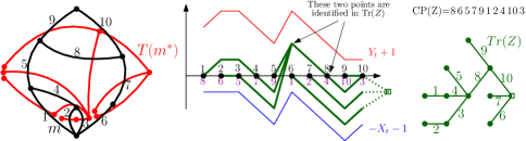
Figure 6: On the left-hand side the map $m$ from Figure 4. In the middle the associated coalescent-walk process $Z=\operatorname{WC}\circ\operatorname{OW}(m)$ that naturally determines the tree $\operatorname{Tr}(Z)$ (shown on the right). Note that the exploration of $\operatorname{Tr}(Z)$ gives the inverse permutation $\operatorname{CP}(Z)^{-1}=6\,7\,10\,8\,3\,2\,4\,1\,5\,9$.

2.5 From plane walks to Baxter permutations via coalescent-walk processes.

We sketch here the proof of Theorem 1.1. The key ingredient is to show that the dual tree $T(m^{*})$ of a bipolar orientation can be recovered from its encoding plane walk by building the associated coalescent-walk process $Z$ and looking at the corresponding tree $\operatorname{Tr}(Z)$. More precisely, let $W=(W_{t})_{1\leq t\leq n}=\operatorname{OW}(m)$ be the walk encoding a given bipolar orientation $m$, and $Z=\operatorname{WC}(W)$ be the corresponding coalescent-walk process. Then the following result, illustrated by an example in Figure 6, holds.

Proposition 2.14.

The tree $\operatorname{Tr}(Z)$ is equal to the dual tree $T(m^{*})$ with edges labeled according to the order given by the exploration of $T(m)$.

The proof requires a lot more notation so we skip it in this extended abstract. Theorem 1.1 then follows immediately, by construction of $\operatorname{OP}(m)$ from $T(m^{*})$ and $T(m)$ (Definition 2.6) and of $\operatorname{CP}(Z)$ from $\operatorname{Tr}(Z)$ (Remark 2.13).

3 Convergence to the Baxter permuton

We start this section by representing a uniform random walk in $\mathcal{W}_{n}$ as a conditioned random walk. For all $n\geq 2$, let $\mathfrak{W}^{A,\mathrm{exc}}_{n}$ be the set of plane walks $(W_{t})_{0\leq t\leq n-1}$ of length $n$ that stay in the non-negative quadrant, starting and ending at $(0,0)$, with increments in $A$ (defined in Equation 4). Remark that for $n\geq 1$, the mapping $\mathcal{\mathfrak{W}}^{A,\mathrm{exc}}_{n+2}\to\mathcal{W}_{n}$ removing the first and the last step, i.e. $W\mapsto(W_{t})_{1\leq t\leq n}$, is a bijection. Recall also that $\bar{\bm{W}}$ denotes the walk defined below Equation 2. An easy calculation then gives the following (observed also in [20, Remark 2]):

Proposition 3.1.

Conditioning on $\{(\bar{\bm{W}}_{t})_{0\leq t\leq{n+1}}\in\mathcal{\mathfrak{W}}^{A,\mathrm{exc}}_{n+2}\}$, the law of $(\bar{\bm{W}}_{t})_{0\leq t\leq n+1}$ is the uniform distribution on $\mathfrak{W}^{A,\mathrm{exc}}_{n+2}$, and the law of $(\bar{\bm{W}}_{t})_{1\leq t\leq n}$ is the uniform distribution on $\mathcal{W}_{n}$.

As we said in the introduction, a key result to prove Theorem 1.5 is to determine the scaling limit of coalescent-walk processes encoded by uniform elements of $\mathcal{W}_{n}$. Thanks to Proposition 3.1 we can equivalently study coalescent-walk processes encoded by quadrant walks conditioned to start and end at $(0,0)$. We will first deal with the unconditioned case (see Section 3.1.1) and then with the conditioned one (see Section 3.1.2).

3.1 Scaling limits of coalescent-walk processes

We start by defining our continuous limiting object: it is formed by the solutions of the following family of stochastic differential equations (SDEs) indexed by $u\in\mathbb{R}$, driven by a two-dimensional process ${\bm{\mathscr{W}}}=({\bm{\mathscr{X}}},{\bm{\mathscr{Y}}})$

$$\begin{cases}d{\bm{\mathscr{Z}}}^{(u)}(t)&=\operatorname{\mathds{1}}_{\{{\bm{\mathscr{Z}}}^{(u)}(t)>0\}}d{\bm{\mathscr{Y}}}(t)-\operatorname{\mathds{1}}_{\{{\bm{\mathscr{Z}}}^{(u)}(t)\leq 0\}}d{\bm{\mathscr{X}}}(t),\quad t\geq u,\\ {\bm{\mathscr{Z}}}^{(u)}(t)&=0,\quad t\leq u.\end{cases}$$ (7)

Existence and uniqueness of solutions were already studied in the literature in the case where the driving process ${\bm{\mathscr{W}}}$ is a Brownian motion, in particular with the following result.

Theorem 3.2 (Theorem 2 of [24], Proposition 2.2 of [9]).

Let $I$ be a (finite or infinite) interval of $\mathbb{R}$ and fix $t_{0}\in I$. Let ${\bm{\mathscr{W}}}=({\bm{\mathscr{X}}},{\bm{\mathscr{Y}}})$ denote a two-dimensional Brownian motion on $I$ with covariance matrix $\begin{pmatrix}1&\rho\\ \rho&1\end{pmatrix}$ for $\rho\in(-1,1)$. We have path-wise uniqueness (explained in 1 below) and existence (explained in 2 below) of a strong solution for the SDE:

$$\begin{cases}d{\bm{\mathscr{Z}}}(t)&=\operatorname{\mathds{1}}_{\{{\bm{\mathscr{Z}}}(t)>0\}}d{\bm{\mathscr{Y}}}(t)-\operatorname{\mathds{1}}_{\{{\bm{\mathscr{Z}}}(t)\leq 0\}}d{\bm{\mathscr{X}}}(t),\quad t\in I\cap[t_{0},+\infty),\\ {\bm{\mathscr{Z}}}(t_{0})&=0.\end{cases}$$ (8)

Namely, letting $(\Omega,\mathcal{F},(\mathcal{F}_{t})_{t\in I},\operatorname{\mathbb{P}})$ be a filtered probability space satisfying the usual conditions, and assuming that $({\bm{\mathscr{X}}},{\bm{\mathscr{Y}}})$ is an $(\mathcal{F}_{t})_{t}$-Brownian motion,

1. if ${\bm{\mathscr{Z}}},{\bm{\mathscr{Z}}}^{\star}$ are two $(\mathcal{F}_{t})_{t}$-adapted continuous processes that verify Equation 8 almost surely, then ${\bm{\mathscr{Z}}}={\bm{\mathscr{Z}}}^{\star}$ almost surely.

2. There exists an $(\mathcal{F}_{t})_{t}$-adapted continuous process ${\bm{\mathscr{Z}}}$ which verifies Equation 8 almost surely, and is adapted to the completion of the canonical filtration of $({\bm{\mathscr{X}}},{\bm{\mathscr{Y}}})$.

3.1.1 The unconditioned scaling limit result

Let us now work on the completed canonical filtered probability space of a Brownian motion ${\bm{\mathscr{W}}}=({\bm{\mathscr{X}}},{\bm{\mathscr{Y}}})$ with covariance $\begin{pmatrix}1&-1/2\\ -1/2&1\end{pmatrix}$. For $u\in\mathbb{R}$, let ${\bm{\mathscr{Z}}}^{(u)}$ be the strong solution of Equation 8 with $I=[u,\infty)$ and $t_{0}=u$, provided by Theorem 3.2. Note that ${\bm{\mathscr{Z}}}^{(u)}$ satisfies Equation 8 (only) for almost all $\omega$. For every $u$, ${\bm{\mathscr{Z}}}^{(u)}$ is adapted, and it is simple to see that the map $(\omega,u)\mapsto{\bm{\mathscr{Z}}}^{(u)}$ is jointly measurable. By Tonelli’s theorem, for almost every $\omega$, ${\bm{\mathscr{Z}}}^{(u)}$ is a solution for almost every $u$.

Remark 3.3.

For fixed $u$, ${\bm{\mathscr{Z}}}^{(u)}$ is a Brownian motion on $[u,\infty)$. Note however that the coupling of ${\bm{\mathscr{Z}}}^{(u)}$ for different values of $u$ is highly non trivial.

Remark 3.4.

Given $\omega$ (even restricted to a set of probability one), we cannot say that $({\bm{\mathscr{Z}}}^{(u)})_{u\in\mathbb{R}}$ forms a whole field of solutions to Equation 7, since we cannot guarantee that the SDE holds for all $u$ simultaneously. Similarly, it is expected that there exists exceptional $u$ where uniqueness fails.

Now, let $\bar{\bm{W}}=(\bar{\bm{X}},\bar{\bm{Y}})=(\bar{\bm{X}}_{k},\bar{\bm{Y}}_{k})_{k\in\mathbb{Z}}$ be the random plane walk defined below Equation 2, and $\bar{\bm{Z}}=\operatorname{WC}(\bar{\bm{W}})$ be the corresponding coalescent-walk process. We define rescaled versions: for all $n\geq 1,u\in\mathbb{R}$, let $\bar{{\bm{\mathscr{W}}}}_{n}:\mathbb{R}\to\mathbb{R}^{2}$ and $\bar{{\bm{\mathscr{Z}}}}^{(u)}_{n}:\mathbb{R}\to\mathbb{R}$ be the continuous functions defined by linearly interpolating the following points:

$$\bar{{\bm{\mathscr{W}}}}_{n}\left(\frac{k}{n}\right)=\frac{1}{\sqrt{2n}}\bar{\bm{W}}_{k},\quad k\in\mathbb{Z},\qquad\bar{{\bm{\mathscr{Z}}}}^{(u)}_{n}\left(\frac{k}{n}\right)=\frac{1}{\sqrt{2n}}\bar{\bm{Z}}^{(\lfloor nu\rfloor)}_{k},\quad u\in\mathbb{R},k\in\mathbb{Z}.$$ (9)

Our most important technical result is the following theorem (whose proof is postponed to Appendix A).

Theorem 3.5.

Let $u_{1}<\ldots<u_{k}$. We have the following joint convergence in $(\mathcal{C}(\mathbb{R},\mathbb{R}))^{k+2}$:

$$\left(\bar{{\bm{\mathscr{W}}}}_{n},\bar{{\bm{\mathscr{Z}}}}^{(u_{1})}_{n},\ldots,\bar{{\bm{\mathscr{Z}}}}^{(u_{k})}_{n}\right)\xrightarrow[n\to\infty]{d}\left({\bm{\mathscr{W}}},{\bm{\mathscr{Z}}}^{(u_{1})},\ldots,{\bm{\mathscr{Z}}}^{(u_{k})}\right).$$ (10)

3.1.2 The conditioned scaling limit result

As a standard application of [12, Theorem 4], the scaling limit of the random walk $\bar{{\bm{\mathscr{W}}}}_{n}$ conditioned on starting at the origin at time 0 and ending at the origin at time $n+1$ is ${\bm{\mathscr{W}}}_{e}=({\bm{\mathscr{X}}}_{e},{\bm{\mathscr{Y}}}_{e})$, the Brownian excursion in the non-negative quadrant of covariance $\begin{pmatrix}1&-1/2\\ -1/2&1\end{pmatrix}$. Let us denote by $(\Omega,\mathcal{F},(\mathcal{F}_{t})_{0\leq t\leq 1},\operatorname{\mathbb{P}}_{\mathrm{exc}})$ the completed canonical probability space of ${\bm{\mathscr{W}}}_{e}$, and work from now on in that space.

It makes sense that the scaling limit of the coalescent-walk process in this conditioned setting should be the solution of Equation 7 driven by ${\bm{\mathscr{W}}}_{e}$, for which we have to show existence and uniqueness. First, let us remark that since Brownian excursions are semimartingales, stochastic integrals are still well-defined. We skip the rather abstract proof of the following, which relies on absolute continuity between Brownian excursion and Brownian motion:

Theorem 3.6.

Denote $\mathcal{F}^{(u)}_{t}=\sigma({\bm{\mathscr{W}}}_{e}(s)-{\bm{\mathscr{W}}}_{e}(u),u\leq s\leq t)$ completed by the $\operatorname{\mathbb{P}}_{\mathrm{exc}}$-negligible sets of $\Omega$. There is a jointly measurable map $(\omega,u)\mapsto{\bm{\mathscr{Z}}}_{e}^{(u)}$ such that for all $u$, ${\bm{\mathscr{Z}}}_{e}^{(u)}$ is $(\mathcal{F}^{(u)}_{t})_{t}$-adapted, and almost surely, for almost every $u$, ${\bm{\mathscr{Z}}}_{e}^{(u)}$ solves Equation 7 driven by ${\bm{\mathscr{W}}}_{e}$. Moreover, for $u\in(0,1)$, if ${\bm{\mathscr{Z}}}^{\star}$ is another $(\mathcal{F}^{(u)}_{t})_{t}$-adapted solution of Equation 7 driven by ${\bm{\mathscr{W}}}_{e}$ started at time $u$, then ${\bm{\mathscr{Z}}}^{\star}={\bm{\mathscr{Z}}}_{e}^{(u)}$ almost surely.

From the above result and the discrete absolutely continuity arguments of [10, 12], we can deduce the following analogous result of Theorem 3.5 (whose proof is omitted). We use the same notation as in Equation 9, and state the result for uniform random times for later convenience.

Theorem 3.7.

Let $\bm{u}_{1}<\ldots<\bm{u}_{k}$ be $k$ sorted independent continuous uniform random variables on $[0,1]$, independent from all other random variables. We have the following convergence in $(\mathcal{C}([0,1],\mathbb{R}))^{k+2}$:

$$\left(\bar{{\bm{\mathscr{W}}}}_{n},\bar{{\bm{\mathscr{Z}}}}^{(\bm{u}_{1})}_{n},\ldots,\bar{{\bm{\mathscr{Z}}}}^{(\bm{u}_{k})}_{n}\Big{|}(\bar{\bm{W}}_{t})_{0\leq t\leq{n+1}}\in\mathcal{\mathfrak{W}}^{A,\mathrm{exc}}_{n+2}\right)\xrightarrow[n\to\infty]{d}\left({\bm{\mathscr{W}}}_{e},{\bm{\mathscr{Z}}}_{e}^{(\bm{u}_{1})},\ldots,{\bm{\mathscr{Z}}}_{e}^{(\bm{u}_{k})}\right).$$

3.2 The construction of the limiting object

We introduce the limiting coalescent Baxter permuton. We place ourselves in the probability space defined above, where ${\bm{\mathscr{W}}}_{e}=({\bm{\mathscr{X}}}_{e},{\bm{\mathscr{Y}}}_{e})$ is a Brownian excursion of correlation $-1/2$ conditioned to stay in the non-negative quadrant. Let ${\bm{\mathscr{Z}}}_{e}=\{{\bm{\mathscr{Z}}}_{e}^{(u)}\}_{u\in[0,1]}$ be the family of processes given by Theorem 3.6, which almost surely solves Equation 7 driven by ${\bm{\mathscr{W}}}_{e}$ for almost every $u$. From the continuous coalescent-walk process ${\bm{\mathscr{Z}}}_{e}$ we build a binary relation $\leq_{{\bm{\mathscr{Z}}}_{e}}$ on $[0,1]$ defined as in Equation 6. Clearly, $(\omega,x,y)\mapsto\operatorname{\mathds{1}}_{x\leq_{{\bm{\mathscr{Z}}}_{e}}y}$ is measurable, and we have the following property whose proof, which relies on path-wise uniqueness, is skipped.

Proposition 3.8.

The relation $\leq_{{\bm{\mathscr{Z}}}_{e}}$ is a total order on $[0,1]\setminus\bm{A}$, where $\bm{A}$ is a random set of zero Lebesgue measure.

We then define the following random function (note that $(\omega,t)\mapsto\varphi_{{\bm{\mathscr{Z}}}_{e}}(t)$ is measurable):

$$\varphi_{{\bm{\mathscr{Z}}}_{e}}(t)\coloneqq\operatorname{Leb}\left(\big{\{}x\in[0,1]|x\leq_{{\bm{\mathscr{Z}}}_{e}}t\big{\}}\right)=\operatorname{Leb}\left(\big{\{}x\in[0,t)|{\bm{\mathscr{Z}}}^{(x)}_{e}(t)<0\big{\}}\cup\big{\{}x\in[t,1]|{\bm{\mathscr{Z}}}^{(t)}_{e}(x)\geq 0\big{\}}\right),$$

where here $\operatorname{Leb}(\cdot)$ denotes the one-dimensional Lebesgue measure. We define the coalescent Baxter permuton as the push-forward of the Lebesgue measure via the map $(\operatorname{Id},\varphi_{{\bm{\mathscr{Z}}}_{e}})$, i.e.

$$\bm{\mu}_{B}(\cdot)=\mu_{{\bm{\mathscr{Z}}}_{e}}(\cdot)\coloneqq(\operatorname{Id},\varphi_{{\bm{\mathscr{Z}}}_{e}})_{*}\operatorname{Leb}(\cdot)=\operatorname{Leb}\left(\{t\in[0,1]|(t,\varphi_{{\bm{\mathscr{Z}}}_{e}}(t))\in\ \cdot\ \}\right).$$

Observation 3.9.

We try to give an intuition behind the definition of $\bm{\mu}_{B}$. Recall that given a coalescent-walk process $Z=\{Z^{(t)}\}_{t\in[n]}\in\mathcal{C}$, we can associate to it the corresponding Baxter permutation $\sigma=\operatorname{CP}(Z)$ and the total order $\leq_{Z}$ on $[n]$. The permutation $\sigma$ satisfies the following property: for every $i\in[n]$, $\sigma(i)=|\{j\in[n]|j\leq_{Z}i\}|.$ The function $\varphi_{{\bm{\mathscr{Z}}}_{e}}$ is a continuous analogue of the permutation $\sigma$, when we consider the continuous coalescent-walk process ${\bm{\mathscr{Z}}}_{e}$ instead of a discrete one, and $\mu_{{\bm{\mathscr{Z}}}_{e}}$ is the associated permuton.

The following result is proved as [21, Proposition 3.1], relying on Proposition 3.8.

Proposition 3.10.

Almost surely, $\mu_{{\bm{\mathscr{Z}}}_{e}}$ is a permuton.

The final proof of Theorem 1.5, i.e. the convergence of uniform Baxter permutations to $\bm{\mu}_{B}$, can be found in Appendix B. We give here a short sketch. The proof is based on the analysis of pattern extraction from uniform Baxter permutations. Proposition 2.12 relates the probability of extracting a specific pattern to the probability that some trajectories of the corresponding coalescent-walk process have given signs at given times. Then, by Theorem 3.7, the latter converges to the analogue probability for the limiting continuous coalescent-walk process.

Appendix A The proof of Theorem 3.5

Recall that $\bar{\bm{W}}=(\bar{\bm{X}},\bar{\bm{Y}})=(\bar{\bm{X}}_{k},\bar{\bm{Y}}_{k})_{k\in\mathbb{Z}}$ is the random plane walk defined below Equation 2, and $\bar{\bm{Z}}=\operatorname{WC}(\bar{\bm{W}})$ is the corresponding coalescent-walk process. We need the following result whose proof is left to the complete version of this extended abstract.

Proposition A.1.

For every $u\in\mathbb{Z}$, $\bar{\bm{Z}}^{(u)}$ has the distribution of a random walk with the same step distribution as $\bar{\bm{Y}}$ (which is the same as that of $-\bar{\bm{X}}$).

Remark A.2.

Recall that the increments of a walk of a coalescent-walk process are not always equal to one of the increments of the corresponding walk (see for instance Equation 5). The statement of Proposition A.1 is a sort of “miracle” of the geometric distribution.

Proof A.3 (Proof of Theorem 3.5).

The first step in the proof is to establish convergence of the components of the vector on the left-hand side of Theorem 3.5. By a classical invariance principle, we get that $\bar{{\bm{\mathscr{W}}}}_{n}=(\bar{{\bm{\mathscr{X}}}}_{n},\bar{{\bm{\mathscr{Y}}}}_{n})$ converges to ${\bm{\mathscr{W}}}=({\bm{\mathscr{X}}},{\bm{\mathscr{Y}}})$ in distribution. Using Proposition A.1, and applying again the invariance principle, we get that $(\bar{{\bm{\mathscr{Z}}}}^{(u)}_{n}({u+t}))_{t\geq 0}$, converges to a one-dimensional Brownian motion. This gives the marginal convergence thanks to Remark 3.3.

The second step in the proof is to establish joint convergence. Marginal convergence gives joint tightness, so that by Prokhorov’s theorem, to show convergence, one only needs to identify the distribution of all joint subsequential limits. Assume that along a subsequence, we have

$$\left(\bar{{\bm{\mathscr{W}}}}_{n},\bar{{\bm{\mathscr{Z}}}}^{(u_{1})}_{n},\ldots,\bar{{\bm{\mathscr{Z}}}}^{(u_{k})}_{n}\right)\xrightarrow[n\to\infty]{d}\left({\bm{\mathscr{W}}},\tilde{{\bm{\mathscr{Z}}}_{1}},\ldots,\tilde{{\bm{\mathscr{Z}}}_{k}}\right).$$

Using Skorokhod’s theorem, we may define all involved variables on the same probability space and assume that the convergence is almost sure. The joint distribution of the right-hand-side is unknown for now, but we will show that for every $1\leq i\leq k$, $\tilde{{\bm{\mathscr{Z}}}_{i}}={\bm{\mathscr{Z}}}^{(u_{i})}$ a.s., which would complete the proof. Recall that ${\bm{\mathscr{Z}}}^{(u_{i})}$ is the strong solution of Equation 8, started at time $u_{i}$ and driven by ${\bm{\mathscr{W}}}=({\bm{\mathscr{X}}},{\bm{\mathscr{Y}}})$, which exists thanks to Theorem 3.2. Let us now fix $i$ and abbreviate $u=u_{i}$, $\tilde{{\bm{\mathscr{Z}}}}=\tilde{{\bm{\mathscr{Z}}}_{i}}$. Our goal is to show that $\tilde{{\bm{\mathscr{Z}}}}$ also verifies Equation 8 and apply path-wise uniqueness.

Let $\mathcal{F}_{t}=\sigma({\bm{\mathscr{W}}}(s),\tilde{{\bm{\mathscr{Z}}}}(s),s\leq t)$. This gives a filtration for which ${\bm{\mathscr{W}}}$ and $\tilde{{\bm{\mathscr{Z}}}}$ are adapted. We will show that ${\bm{\mathscr{W}}}$ is an $(\mathcal{F}_{t})_{t}$-Brownian motion, that is for $t\in\mathbb{R},s\geq 0$, $({\bm{\mathscr{W}}}(t+s)-{\bm{\mathscr{W}}}(t))\perp\!\!\!\perp\mathcal{F}_{t}$. For fixed $n$, by definition of a random walk, $\bar{{\bm{\mathscr{W}}}}_{n}({t+s})-\bar{{\bm{\mathscr{W}}}}_{n}(t)$ is independent from $\sigma(\bar{\bm{W}}_{k},k\leq\lfloor nt\rfloor)$. Therefore, by the definition given in Equation 5,

$$\left(\bar{{\bm{\mathscr{W}}}}_{n}({t+s})-\bar{{\bm{\mathscr{W}}}}_{n}(t)\right)\ \perp\!\!\!\perp\ \left(\bar{{\bm{\mathscr{W}}}}_{n}(r),\bar{{\bm{\mathscr{Z}}}}^{(u)}_{n}(r)\right)_{r\leq n^{-1}\lfloor nt\rfloor}.$$ (11)

By convergence, we obtain that ${\bm{\mathscr{W}}}(t+s)-{\bm{\mathscr{W}}}(t)$ is independent from $\left({\bm{\mathscr{W}}}(r),\tilde{{\bm{\mathscr{Z}}}}(r)\right)_{r\leq t}$, completing the claim that ${\bm{\mathscr{W}}}$ is an $(\mathcal{F}_{t})_{t}$-Brownian motion.

Now fix a rational $\varepsilon>0$ and a rational $t>u$ such that $\tilde{{\bm{\mathscr{Z}}}}(t)>\varepsilon$. There is $\delta>0$ so that $\tilde{{\bm{\mathscr{Z}}}}>\varepsilon/2$ on $[t-\delta,t+\delta]$. By almost sure convergence, there is $N_{0}$ such that for $n\geq N_{0}$, $\bar{{\bm{\mathscr{Z}}}}^{(u)}_{n}>\varepsilon/4$ on $[t-\delta,t+\delta]$. On this interval, outside of the event

$$\{\sup_{1\leq i\leq n}|\bar{{\bm{\mathscr{Y}}}}_{i}-\bar{{\bm{\mathscr{Y}}}}_{i-1}|\geq\sqrt{2n}\varepsilon/4\},$$

$\bar{{\bm{\mathscr{Z}}}}^{(u)}_{n}-\bar{{\bm{\mathscr{Y}}}}_{n}$ is constant by construction of the coalescent-walk process. As a result (the probability of the bad event is bounded by $Ce^{-c\sqrt{n}}$ ), the limit $\tilde{{\bm{\mathscr{Z}}}}-{\bm{\mathscr{Y}}}$ is constant too almost surely. We have shown that almost surely $\tilde{{\bm{\mathscr{Z}}}}-{\bm{\mathscr{Y}}}$ is locally constant on $\{t:\tilde{{\bm{\mathscr{Z}}}}(t)>\varepsilon\}$. This translates into the following equality:

$$\int_{u}^{t}\operatorname{\mathds{1}}_{\{\tilde{{\bm{\mathscr{Z}}}}(r)>\varepsilon\}}d\tilde{{\bm{\mathscr{Z}}}}(r)=\int_{u}^{t}\operatorname{\mathds{1}}_{\{\tilde{{\bm{\mathscr{Z}}}}(r)>\varepsilon\}}d{\bm{\mathscr{Y}}}(r).$$

The stochastic integrals are well-defined: on the left-hand side by considering the canonical filtration of $\tilde{{\bm{\mathscr{Z}}}}$, on the right-hand-side by considering $(\mathcal{F}_{t})_{t}$. The same can be done for negative values, leading to

$$\int_{u}^{t}\operatorname{\mathds{1}}_{\{|\tilde{{\bm{\mathscr{Z}}}}(r)|>\varepsilon\}}d\tilde{{\bm{\mathscr{Z}}}}(r)=\int_{u}^{t}\operatorname{\mathds{1}}_{\{\tilde{{\bm{\mathscr{Z}}}}(r)>\varepsilon\}}d{\bm{\mathscr{Y}}}(r)-\int_{u}^{t}\operatorname{\mathds{1}}_{\{\tilde{{\bm{\mathscr{Z}}}}(r)<-\varepsilon\}}d{\bm{\mathscr{X}}}(r).$$

By stochastic dominated convergence theorem [25, Thm. IV.2.12], one can take the limit as $\varepsilon\to 0$, and obtain

$$\int_{u}^{t}\operatorname{\mathds{1}}_{\{\tilde{{\bm{\mathscr{Z}}}}(r)\neq 0\}}d\tilde{{\bm{\mathscr{Z}}}}(r)=\int_{u}^{t}\operatorname{\mathds{1}}_{\{\tilde{{\bm{\mathscr{Z}}}}(r)>0\}}d{\bm{\mathscr{Y}}}(r)-\int_{u}^{t}\operatorname{\mathds{1}}_{\{\tilde{{\bm{\mathscr{Z}}}}(r)<0\}}d{\bm{\mathscr{X}}}(r).$$

Thanks to the fact that $\tilde{{\bm{\mathscr{Z}}}}$ is Brownian, $\int_{u}^{t}\operatorname{\mathds{1}}_{\{\tilde{{\bm{\mathscr{Z}}}}(r)=0\}}d\tilde{{\bm{\mathscr{Z}}}}(r)=0$, so that the left-hand side equals $\tilde{{\bm{\mathscr{Z}}}}(t)$. As a result $\tilde{{\bm{\mathscr{Z}}}}$ verifies Equation 8 and we can apply path-wise uniqueness (Theorem 3.2) to complete the proof.

Appendix B The proof of Theorem 1.5

Recall that permuton convergence has been defined in Definition 1.4. We present one its characterizations (which comes from [1, Theorem 2.5]), expressed in terms of random induced patterns. For $n\in\mathbb{Z}_{>0}$, we denote by $\mathfrak{S}_{n}$ the set of permutations of size $n$. Let $1\leq k\leq n$, $\sigma\in\mathfrak{S}_{n}$ and $I=\{i_{1},\ldots i_{k}\}$ with $1\leq i_{1}<\dots<i_{k}\leq n$. The pattern in $\sigma$ induced by $I$ is the only permutation $\pi\in\mathfrak{S}_{k}$ such that the $k$ values $\sigma(i_{1}),\dots,\sigma(i_{k})$ are order isomorphic to $\pi(1),\dots,\pi(k)$. In this case, we write $\operatorname{pat}_{I}(\sigma)=\pi$.

We also define permutations induced by $k$ points in the square $[0,1]^{2}$. Take a sequence of $k$ points $(X,Y)=((x_{1},y_{1}),\dots,(x_{k},y_{k}))$ in $[0,1]^{2}$ in general position, i.e. with distinguished $x$ and $y$ coordinates. We denote by $(x_{(1)},y_{(1)}),\dots,(x_{(k)},y_{(k)})$ the $x$-reordering of $(X,Y)$, i.e. the unique reordering of the sequence $((x_{1},y_{1}),\dots,(x_{k},y_{k}))$ such that $x_{(1)}<\cdots<x_{(k)}$. Then the values $(y_{(1)},\ldots,y_{(k)})$ are in the same relative order as the values of a unique permutation, that we call the permutation induced by $(X,Y)$.

Proposition B.1.

Let $\bm{\sigma}_{n}$ be a random permutation of size $n$, and $\bm{I}_{n}^{k}=\{\bm{i}^{1}_{n},\dots,\bm{i}^{k}_{n}\}$ be a uniform $k$-element subset of $[n]$, independent of $\bm{\sigma}_{n}$. Let $\bm{\mu}$ be a random permuton, and denote $\operatorname{Perm}_{k}(\bm{\mu})$ the unique permutation induced by $k$ independent points in $[0,1]^{2}$ with common distribution $\bm{\mu}$ conditionally on $\bm{\mu}$. Then

$$\mu_{\bm{\sigma}_{n}}\stackrel{{\scriptstyle d}}{{\to}}\bm{\mu}\iff\forall k\in\mathbb{Z}_{>0},\;\forall\pi\in\mathfrak{S}_{k},\quad\operatorname{\mathbb{P}}(\operatorname{pat}_{\bm{I}_{n}^{k}}(\bm{\sigma}_{n})=\pi)\to\operatorname{\mathbb{P}}(\operatorname{Perm}_{k}(\bm{\mu})=\pi).$$

We can now prove Theorem 1.5. First we state a consequence of the fact that $\mu_{{\bm{\mathscr{Z}}}_{e}}$ is a permuton and that ${\bm{\mathscr{Z}}}_{e}^{(s)}(t)$ are continuous random variables, which allows us to get rid of equalities:

Lemma B.2.

Almost surely, for almost every $s<t\in[0,1]$, ${\bm{\mathscr{Z}}}_{e}^{(s)}(t)\neq 0$. Then ${\bm{\mathscr{Z}}}_{e}^{(s)}(t)>0$ implies $\varphi_{{\bm{\mathscr{Z}}}_{e}}(s)<\varphi_{{\bm{\mathscr{Z}}}_{e}}(t)$, and ${\bm{\mathscr{Z}}}_{e}^{(s)}(t)<0$ implies $\varphi_{{\bm{\mathscr{Z}}}_{e}}(s)>\varphi_{{\bm{\mathscr{Z}}}_{e}}(t)$.

Proof B.3 (Proof of Theorem 1.5).

We reuse here the notation of Theorem 3.7. In particular $\bar{\bm{W}}$ is a $\nu$-random walk and $\bar{\bm{Z}}=\operatorname{WC}(\bar{\bm{W}})$ is the associated coalescent-walk process. Let $\bm{\sigma}_{n}=\operatorname{CP}(\bar{\bm{Z}}|_{[n]})$. Let $\mathcal{E}_{n}$ denote the event $\{(\bar{\bm{W}}_{t})_{0\leq t\leq{n+1}}\in\mathcal{\mathfrak{W}}^{A,\mathrm{exc}}_{n+2}\}$. By Proposition 3.1 and the fact that the mapping $\operatorname{CP}\circ\operatorname{WC}$ is a size-preserving bijection, conditioned on $\mathcal{E}_{n}$, $\bm{\sigma}_{n}$ is a uniform Baxter permutation.

Fix $k\geq 1$ and $\pi\in\mathfrak{S}_{k}$. For $n\geq k$, let $\bm{I}_{n}=\{\bm{i}^{1}_{n},\dots,\bm{i}^{k}_{n}\}$ be a uniform $k$-element subset of $[n]$, independent of $\bm{\sigma}_{n}$. In view of Proposition B.1, to complete the proof, we will show that

$$\operatorname{\mathbb{P}}(\operatorname{pat}_{\bm{I}_{n}}(\bm{\sigma}_{n})=\pi\mid\mathcal{E}_{n})\xrightarrow[n\to\infty]{}\operatorname{\mathbb{P}}(\operatorname{Perm}_{k}(\mu_{{\bm{\mathscr{Z}}}_{e}})=\pi).$$

Thanks to Proposition 2.12, we have

$$\operatorname{\mathbb{P}}(\operatorname{pat}_{\bm{I}_{n}}(\bm{\sigma}_{n})=\pi\mid\mathcal{E}_{n})=\operatorname{\mathbb{P}}\Big{(}\forall_{1\leq\ell<s\leq k},\,\bar{\bm{Z}}^{(\bm{i}^{\ell}_{n})}_{\bm{i}^{s}_{n}}\geq 0\iff\pi(\ell)>\pi(s)\mid\mathcal{E}_{n}\Big{)}.$$

Let $(\bm{u}_{1},\dots,\bm{u}_{k})$ be the sorted vector of $k$ independent uniform continuous random variables in $[0,1]$. For every $n\geq 1$, one can couple $\bm{I}_{n}$ and $(\bm{u}_{1},\dots,\bm{u}_{k})$ so that $\bm{i}_{n}^{j}=\lfloor n\bm{u}_{j}\rfloor$ for every $1\leq j\leq k$, with an error of probability $O(1/n)$. As a result,

$$\operatorname{\mathbb{P}}(\operatorname{pat}_{\bm{I}_{n}}(\bm{\sigma}_{n})=\pi\mid\mathcal{E}_{n})= \operatorname{\mathbb{P}}\Big{(}\forall_{1\leq\ell<s\leq k},\,(2n)^{-1/2}\bar{\bm{Z}}^{(\bm{u}_{\ell})}_{\bm{u}_{s}}\geq 0\iff\pi(\ell)>\pi(s)\mid\mathcal{E}_{n}\Big{)}+O(1/n)$$

$$\xrightarrow[n\to\infty]{} \operatorname{\mathbb{P}}\Big{(}\forall_{1\leq\ell<s\leq k},\,{\bm{\mathscr{Z}}}^{(\bm{u}_{\ell})}_{e}({\bm{u}_{s}})\geq 0\iff\pi(\ell)>\pi(s)\Big{)}$$

$$= \operatorname{\mathbb{P}}\left(\forall_{1\leq\ell<s\leq k},\begin{cases}\pi(\ell)>\pi(s)\implies\varphi_{{\bm{\mathscr{Z}}}_{e}}(\bm{u}_{\ell})>\varphi_{{\bm{\mathscr{Z}}}_{e}}(\bm{u}_{s})\\ \pi(\ell)<\pi(s)\implies\varphi_{{\bm{\mathscr{Z}}}_{e}}(\bm{u}_{\ell})<\varphi_{{\bm{\mathscr{Z}}}_{e}}(\bm{u}_{s})\end{cases}\right),$$ (12)

where for the limit we used the convergence in distribution of Theorem 3.7 together with the Portmanteau theorem. Additionally, Lemma B.2 is used both to take care of the boundary effect in the Portmanteau theorem, and to do the rewriting in the last line.

In order to finish the proof, it is enough to check that the probability on the right-hand side of Equation 12 equals $\operatorname{\mathbb{P}}(\operatorname{Perm}_{k}(\mu_{{\bm{\mathscr{Z}}}_{e}})=\pi)$. This is clear since by definition of $\operatorname{Perm}_{k}$ and $\mu_{{\bm{\mathscr{Z}}}_{e}}$, $\operatorname{Perm}_{k}(\mu_{{\bm{\mathscr{Z}}}_{e}})$ is the permutation induced by $\big{(}(\bm{u}_{1},\varphi_{{\bm{\mathscr{Z}}}_{e}}(\bm{u}_{1})),\dots,(\bm{u}_{k},\varphi_{{\bm{\mathscr{Z}}}_{e}}(\bm{u}_{k}))\big{)}.$

Appendix C Simulations of large Baxter permutations

The simulations for Baxter permutations presented in the first page of this extended abstract have been obtained in the following way:

1. first, we have sampled a uniform random walk of size $n+2$ in the non-negative quadrant starting at $(0,0)$ and ending at $(0,0)$ with increments distribution given by Equation 2. This has been done using a "rejection algorithm": it is enough to sample a walk $W$ starting at $(0,0)$ with increments distribution given by Equation 2, up to the first time it leaves the non-negative quadrant. Then one has to check if the last step inside the non-negative quadrant is at the origin $(0,0)$. When this is the case (otherwise we resample a new walk), the part of the walk $W$ inside the non-negative quadrant, denoted $\tilde{W}$, is a uniform walk of size $|\tilde{W}|$ in the non-negative quadrant starting at $(0,0)$ and ending at $(0,0)$ with increments distribution given by Equation 2.

2. Removing the first and the last step of $\tilde{W}$, thanks to Proposition 3.1, we obtained a uniform random walk in $\mathcal{W}_{n}$.

3. Finally, applying the mapping $\operatorname{CP}\circ\operatorname{WC}$ to the walk given by the previous step, we obtained a uniform Baxter permutation of size $n$ (thanks to Theorem 1.1).

Note that our algorithm gives a uniform Baxter permutation of random size.

References

- [1] F. Bassino, M. Bouvel, V. Féray, L. Gerin, M. Maazoun, and A. Pierrot. Universal limits of substitution-closed permutation classes. Journal of the European Mathematical Society, to appear, 2019.
- [2] F. Bassino, M. Bouvel, V. Féray, L. Gerin, and A. Pierrot. The Brownian limit of separable permutations. The Annals of Probability, 46(4):2134–2189, 2018.
- [3] G. Baxter. On fixed points of the composite of commuting functions. Proc. Amer. Math. Soc., 15:851–855, 1964. URL: https://doi.org/10.2307/2034894, doi:10.2307/2034894.
- [4] I. Benjamini and O. Schramm. Recurrence of distributional limits of finite planar graphs. Electron. J. Probab., 6:no. 23, 13, 2001. URL: https://doi.org/10.1214/EJP.v6-96, doi:10.1214/EJP.v6-96.
- [5] N. Bonichon, M. Bousquet-Mélou, and É. Fusy. Baxter permutations and plane bipolar orientations. Sém. Lothar. Combin., 61A:Art. B61Ah, 29, 2009/11.
- [6] J. Borga. Local convergence for permutations and local limits for uniform -avoiding permutations with . Probability Theory and Related Fields, 176(1):449–531, 2020. doi:https://doi.org/10.1007/s00440-019-00922-4.
- [7] J. Borga, M. Bouvel, V. Féray, and B. Stufler. A decorated tree approach to random permutations in substitution-closed classes. arXiv preprint:1904.07135, 2019.
- [8] J. Borga and E. Slivken. Square permutations are typically rectangular. Annals of Applied Probability, to appear, 2019.
- [9] M. Çağlar, H. Hajri, and A. H. Karakuş. Correlated coalescing Brownian flows on and the circle. ALEA Lat. Am. J. Probab. Math. Stat., 15(2):1447–1464, 2018.
- [10] D. Denisov and V. Wachtel. Random walks in cones. Ann. Probab., 43(3):992–1044, 2015. URL: https://doi.org/10.1214/13-AOP867, doi:10.1214/13-AOP867.
- [11] T. Dokos and I. Pak. The expected shape of random doubly alternating Baxter permutations. Online J. Anal. Comb., 9:12, 2014.
- [12] J. Duraj and V. Wachtel. Invariance principles for random walks in cones. arXiv preprint:1508.07966, 2015.
- [13] S. Felsner, É. Fusy, M. Noy, and D. Orden. Bijections for Baxter families and related objects. J. Combin. Theory Ser. A, 118(3):993–1020, 2011. URL: https://doi.org/10.1016/j.jcta.2010.03.017, doi:10.1016/j.jcta.2010.03.017.
- [14] E. Gwynne, N. Holden, and X. Sun. Joint scaling limit of a bipolar-oriented triangulation and its dual in the Peanosphere sense. arXiv preprint:1603.01194, 2016.
- [15] E. Gwynne, N. Holden, and X. Sun. A mating-of-trees approach for graph distances in random planar maps. arXiv preprint arXiv:1711.00723, 2017.
- [16] E. Gwynne, N. Holden, and X. Sun. Mating of trees for random planar maps and Liouville quantum gravity: a survey. arXiv preprint:1910.04713, 2019.
- [17] C. Hoffman, D. Rizzolo, and E. Slivken. Scaling limits of permutations avoiding long decreasing sequences. arXiv preprint:1911.04982, 2019.
- [18] C. Hoppen, Y. Kohayakawa, C. G. Moreira, B. Ráth, and R. M. Sampaio. Limits of permutation sequences. Journal of Combinatorial Theory, Series B, 103(1):93–113, 2013.
- [19] R. Kenyon, D. Král’, C. Radin, and P. Winkler. Permutations with fixed pattern densities. Random Structures & Algorithms, 2019. URL: https://onlinelibrary.wiley.com/doi/abs/10.1002/rsa.20882, arXiv:https://onlinelibrary.wiley.com/doi/pdf/10.1002/rsa.20882, doi:10.1002/rsa.20882.
- [20] R. Kenyon, J. Miller, S. Sheffield, and D. B. Wilson. Bipolar orientations on planar maps and . Ann. Probab., 47(3):1240–1269, 2019. URL: https://doi.org/10.1214/18-AOP1282, doi:10.1214/18-AOP1282.
- [21] M. Maazoun. On the Brownian separable permuton. Combinatorics, Probability and Computing, page 1–26, 2019. doi:10.1017/S0963548319000300.
- [22] N. Madras and H. Liu. Random pattern-avoiding permutations. Algorithmic Probability and Combinatorics, AMS, Providence, RI, pages 173–194, 2010.
- [23] S. Miner and I. Pak. The shape of random pattern-avoiding permutations. Adv. in Appl. Math., 55:86–130, 2014. URL: http://dx.doi.org/10.1016/j.aam.2013.12.004, doi:10.1016/j.aam.2013.12.004.
- [24] V. Prokaj. The solution of the perturbed Tanaka-equation is pathwise unique. Ann. Probab., 41(3B):2376–2400, 2013. URL: https://doi.org/10.1214/11-AOP716, doi:10.1214/11-AOP716.
- [25] D. Revuz and M. Yor. Continuous martingales and Brownian motion, volume 293. Springer Science & Business Media, 2013.