Crystal Structure Prediction via Oblivious Local Search
2Leverhulme Research Centre for Functional Materials Design, UK
3Department of Computer Science, Royal Holloway University of London, UK
4Department of Computer Science, University of Liverpool, UK
5Computer Engineering and Informatics Department, University of Patras, Greece
Email: {D.Antypov, Vladimir.Gusev, M.J.Rosseinsky, P.Spirakis, Michail.Theofilatos}@liverpool.ac.uk, Argyrios.Deligkas@rhul.ac.uk )
Abstract
We study Crystal Structure Prediction, one of the major problems in computational chemistry. This is essentially a continuous optimization problem, where many different, simple and sophisticated, methods have been proposed and applied. The simple searching techniques are easy to understand, usually easy to implement, but they can be slow in practice. On the other hand, the more sophisticated approaches perform well in general, however almost all of them have a large number of parameters that require fine tuning and, in the majority of the cases, chemical expertise is needed in order to properly set them up. In addition, due to the chemical expertise involved in the parameter-tuning, these approaches can be biased towards previously-known crystal structures. Our contribution is twofold. Firstly, we formalize the Crystal Structure Prediction problem, alongside several other intermediate problems, from a theoretical computer science perspective. Secondly, we propose an oblivious algorithm for Crystal Structure Prediction that is based on local search. Oblivious means that our algorithm requires minimal knowledge about the composition we are trying to compute a crystal structure for. In addition, our algorithm can be used as an intermediate step by any method. Our experiments show that our algorithms outperform the standard basin hopping, a well studied algorithm for the problem.
Keywords: crystal structure prediction; local search; combinatorial neighborhood.
1 Introduction
The discovery of new materials has historically been made by experimental investigation guided by chemical understanding. This approach can be both time consuming and challenging because of the large space to be explored. For example, a “traditional” method for discovering inorganic solid structures relies on knowledge of crystal chemistry coupled with repeating synthesis experiments and systematically varying elemental ratios, each of which can take lots of time [24, 25]. As a result there is a very large unexplored space of chemical systems: only of binary systems, of ternary, and just of quaternary systems have been studied experimentally [26].
These inefficiencies forced physical scientists to develop computational approaches in order to tackle the problem of finding new materials. The first approach is based on data mining where only pre-existing knowledge is used [6, 10, 12, 14, 22]. Although this approach has proven to be successful, there is the underlying risk of missing best-in-class materials by being biased towards known crystal structures. Hence, the second approach tries to fill this gap and aims at finding new materials with little, or no, pre-existing knowledge, by predicting the crystal structure of the material. This approach has led to the discovery of several new, counterintuitive, materials whose existence could not be deduced by the structures of previously-known materials [5].
Several heuristic methods have been suggested for crystal structure prediction. All these methods are based on the same fundamental principle. Every arrangement of ions in the 3-dimensional Euclidean space corresponds to an energy value and it defines a point on the potential energy surface. Then, the crystal structure prediction problem is formulated as a mathematical optimization problem where the goal is to compute the structure that corresponds to the global minimum of the potential energy surface, since this is the most likely structure that corresponds to a stable material. The difficulties in solving this optimization problem is that the potential energy surface is highly non convex, with exponentially many, with respect to the number of ions, local minima [16]. For this reason, several different algorithmic techniques were proposed ranging from simple techniques, like quasi-random sampling [8, 20, 19, 21], basin hopping [11, 27], and simulated annealing techniques [17, 23], to more sophisticated techniques, like evolutionary and genetic algorithms [3, 7, 13, 15, 29], and tiling approaches [5, 4]. A recent comprehensive review on these techniques can be found in [16].
The simple searching techniques are easy to understand, usually easy to implement, and they are unbiased, but they can be slow in practice. On the other hand, the more sophisticated approaches perform well in general, however almost all of them have a large number of parameters that require fine tuning and, in the majority of the cases, chemical expertise is needed in order to properly set them up. In addition, due to the chemical expertise involved in the parameter-tuning, these approaches can be biased towards previously-known structures.
The majority of the abovementioned heuristic techniques work, at a very high level, in a similar way. Given a current solution for the crystal structure prediction problem, i.e., a location for every ion in the 3-dimensional space, they iteratively perform the following three steps.
-
1.
Choose a new potential solution . This can be done by taking into account, or modifying, .
-
2.
Perform gradient descent on the potential energy surface starting from , until a local minimum is found. This process is called relaxation of .
-
3.
Decide whether to keep as the candidate solution or to update it to the solution found after relaxing .
For example, basin hopping algorithms randomly choose , they relax and if the energy of the relaxed structure is lower than the , or a Metropolis criterion is satisfied, they accept this as a current solution; else they keep and they randomly choose . The procedure usually stops when the algorithm fails to find a structure with lower energy within a predefined number of iterations. The more sophisticated algorithms take into account knowledge harvested from chemists and put constraints on the way is selected. For example, the MC-EMMA [5] and the FUSE [4] algorithms use a set of building blocks to construct . These building blocks are local configurations of ions that are present in, or similar to, known crystal structures. These approaches restrict the search space ,which accelerate search, but reduce the number of possible solutions.
This general algorithm is easy to understand, however there are some hidden difficulties that make the problem more challenging. Firstly, it is not trivial even how to evaluate the potential energy of a structure. There are several different methods for calculating the energy of a structure, ranging from quantum mechanical methods, like density functional theory 111https://en.wikipedia.org/wiki/Density_functional_theory, to force fields methods 222https://en.wikipedia.org/wiki/Force_field_(chemistry), like the Buckingham-Coulomb potential function. All of which though, are hard to compute (see Section 2.1) from the point of view of (theoretical) computer science and thus only numerical methods are known and used in practice for them [9]; still there are cases where some methods need considerable time to calculate the energy of a structure. This yields another, more important, difficulty, the relaxation of a structure. Since it is hard to compute the energy of a structure, it is even harder to apply gradient descent on the potential energy surface. For these reasons, the majority of the heuristic algorithms depend on external, well established, codes [9] for computing the aforementioned quantities. Put differently, both energy computations and relaxations of structures are treated as oracles or black boxes.
1.1 Our contribution.
Our contribution is twofold. Firstly, we formalize the Crystal Structure Prediction problem from the theoretical computer science perspective; to the best of our knowledge, this is among the few papers that attempt to connect computational chemistry and computer science. En route to this, we introduce several intermediate open problems from computational chemistry in CS terms. Any (partial) positive solution to these questions can significantly help computational chemists to identify new materials. On the other hand, any negative result can formally explain why the discovery of new materials is a notoriously difficult task.
Our second contribution is the partial answer for some of the questions we cast. In general, our goal is to create oblivious algorithms that are easy to implement, they are fast, and they work well in practice. With oblivious we mean that we are seeking for general procedures that require minimal input and they have zero, or just a few, parameters chosen by the user.
-
•
We propose a purely combinatorial method for estimating the energy of a structure, which we term depth energy computation. We choose to compare our method against GULP [9], which is considered to be the state of the art for computing the energy of a structure and for performing relaxations when the Buckingham-Coulomb energy is used. Our method requires only the charges of the atoms and their corresponding Buckingham coefficients to work; see Eq. 2 in Section 2.1. In addition, it needs only one parameter, the depth . We experimentally demonstrate that our method monotonically approximates with respect to the energy computed by GULP and that it achieves an error of for . Our experiments show that the structure that achieves the minimum energy in depth 1 is likely to be the structure with the minimum energy overall. In fact we show something much stronger. If the energy of is lower than the energy of when it is computed via the depth energy computation for , then, almost always, the energy of will be lower than the energy of when it is computed via GULP.
-
•
We derive oblivious algorithms for choosing which structure to relax next. All of our algorithms are based on local search. More formally, starting with and using only local changes we select . We define several “combinatorial neighborhoods” and we evaluate their efficiency. Our neighborhoods are oblivious since they only need access to an oracle that calculates the energy of a structure. We show that our method outperforms basin hopping. Moreover, we view our algorithms as an intermediate step before relaxation that can be applied to any existing algorithm.
2 Preliminaries
A crystal is a solid material whose atoms are arranged in a highly ordered configuration, forming a crystal structure that extends in all directions. A crystal structure is characterized by its unit cell; a parallelepiped that contains atoms in a specific arrangement. The unit cell is the period of the crystal; unit cells are stacked in the three dimensional space to form the crystal. In this paper we focus on ionically bonded crystals, which we describe next; what follows is relevant only on crystals of this type. In order to fully define the unit cell of a ionically bonded crystal structure, we have to specify a composition, unit cell parameters, and an arrangement of the ions.

Composition.
A composition is the chemical formula that describes the ratio of ions that belong to the unit cell. The chemical formula contains anions, negatively charged ions, and cations, positively charged ions. The chemical formula is a way of presenting information about the chemical proportions of ions that constitute a particular chemical compound, and it does not provide any information about the exact number of atoms in the unit cell. More formally, the composition is defined by a set of distinct chemical elements , their multiplicity , and a non-zero integer charge for each element . The number denotes the total number of distinct chemical elements, and is the proportion of the atoms of type in the unit cell. It is required that the sum of the charges adds up to zero, i.e. , , so that the unit cell is charge neutral. For example, the composition for Strontium Titanate, , denotes that the following hold. For every ion of strontium (Sr) in the unit cell, there exists one ion of titanium (Ti) and three ions of oxygen (O). Furthermore, the charge of every ion of Sr is , of Ti is , and of O is . Hence, when the ratios of the ions are according to the composition, the charge of the unit cell is zero.
Another parameter for every atom is the atomic radius. This usually corresponds to the distance from the center of the nucleus to the boundary of the surrounding shells of electrons. Since the boundary is not a well-defined physical entity, there are various non-equivalent definitions of atomic radius. In crystal structures though, the ionic radius is used and usually is treated as a hard sphere. Thus, we will use to denote the ionic radius of the element .
Unit cell parameters.
Unit cell parameters provide a formal description of the parallelepiped that represents the unit cell. These include the lengths of the parallelepiped in every dimension and the angles , , and between the corresponding facets. For brevity, we denote and , and we use to denote the unit cell parameters.
Arrangement.
An arrangement describes the position of each atom of the composition in the unit cell. The position of ion is specified by a point in the parallelepiped defined by the unit cell parameters; fractional coordinates denote the location of the nucleus of the ion in the unit cell. A unit cell parameters-arrangement combination in a unit cell with ions is a point in the -dimensional space. For any two points and we will use to denote their Euclidean distance.
As we have already said, a unit cell parameters-arrangement configuration defines the period of an infinite structure that covers the whole 3d space. To get some intuition, assume that we have an orthogonal unit cell, i.e., all the angles are 90 degrees. Then for every ion with position in the unit cell, there exist “copies” of the ion in the positions for every possible combination of integers , and . A unit cell parameters-arrangement configuration is feasible if the hard spheres of any two ions of the crystal structure do not overlap; formally, it is feasible if for every two ions and it holds that .
2.1 Energy
Any unit cell parameters-arrangement configuration of a composition corresponds to a potential energy. When the number of ions in the unit cell is fixed, the set of configurations define the potential energy surface.
Buckingham-Coulomb potential is among the most well adopted methods for computing energy [2, 28] and it is the sum of the Buckingham potential and the Coulomb potential. The Coulomb potential is long-range and depends only on the charges and the distance between the ions; for a pair of ions and , the Coulomb energy is defined by
| (1) |
Note, ions and can be in different unit cells.
The Buckingham potential is short-range and depends on the species of the ions and their distance. More formally, it depends on positive composition-dependent constants , and for every pair of species and ; here can be equal to 333The Buckingham constants are composition-depended since they can have small discrepancies in different compositions. For example the constants , and for can be different than those for . There is a long line of research in computational chemistry that tries to learn/estimate the Buckingham constants for various compositions. In addition, more than one set of Buckingham constants can be available for a given composition.. So, for the pair of ions , of specie , and , of specie , the Buckingham energy is
| (2) |
Again, ions and can be in different unit cells.
Let denote the sphere with centre and radius . The total energy of a crystal structure whose unit cell is characterized by ions with arrangement is then defined
conditionally converges to a certain value [18] and usually numerical approaches are used to compute it. For this reason, and since we aim for an oblivious algorithm, we view the computation of the energy of a structure as a black box. More specifically, we assume that we have an oracle that given any structure , it returns its corresponding energy.
Open Question 1.
Given a composition and Buckingham parameters for it, find a simple, purely combinatorial way that approximates the energy for every crystal structure.
Open Question 2.
Given a composition and an oracle that computes the energy of every structure for this composition, learn efficiently (with respect to the number of oracle calls) the Buckingham parameters , and for every .
Relaxation.
The relaxation of a crystal structure computes a stationary point on the potential energy surface by applying gradient descent starting from . The relaxation of a structure can change both the arrangement of the ions in the unit cell and the unit cell parameters of the unit cell. We follow a similar approach as we did with the energy and we assume that there is an oracle that given a crystal structure it returns the relaxed structure.
Open Question 3.
Find an alternative, quicker, way to compute an approximate local minimum when:
-
a)
the unit cell parameters of the unit cell are fixed;
-
b)
the arrangement of the ions is fixed;
-
c)
both unit cell parameters and arrangement are free.
2.2 Crystal Structure Prediction problems
In crystal structure prediction problems the general goal is to minimize the energy in the unit cell. There are two kinds of problems we are concerned. The first cares only about the value of the energy and the second one cares for the arrangement and the unit cell parameters that achieve the minimum energy. From the computational chemistry point of view, both questions are interesting in their own right. The existence of a unit cell parameters-arrangement that achieves lower-than-currently-known energy usually suffices for constructing a new material. On the other hand, identifying the arrangement and the unit cell parameters of a crystal structure that achieves the lowest possible energy can help physical scientists to predict the properties of the material.
The second class of problems, the ones that ultimately computational chemists would like to solve, take as input only the composition and the goal is to construct a unit cell, with any number of atoms, such that the average energy per ion is minimized.
Although the problems are considered to be intractable [16], only recently the first correct NP-hardness result was proven for a variant of CSP [1]. However, for the problems presented, there are no correct NP-hardness results in the literature.
Open Question 4.
Provide provable lower bounds and upper bounds for the four problems defined above.
Open Question 5.
Construct a heuristic algorithm that works well in practice.
3 Local Search
Local search algorithms start from a feasible solution and iteratively obtain better solutions. The key concept for the success of such algorithms, is given a feasible solution, to be able to efficiently find an improved one. Put formally, a local search algorithm is defined by a neighbourhood function and a local rule . In every iteration, the algorithm does the following.
-
•
Has the current best solution .
-
•
Computes the neighbourhood .
-
•
If there is an improved solution in , then it updates according to the rule , i.e. ; else it terminates and outputs .
The neighborhood of a solution consists of all feasible solutions that are “close” in some sense to . The size of the neighborhood can be constant or a function of the input. In principle, the larger the size of the neighborhood, the better the quality of the locally optimal solutions. However, the downside of choosing large neighborhoods is that, in general, it makes each iteration computationally more expensive. Running time and quality of solutions are competing considerations, and the trade off between them can be determined through experimentation.
We study the following combinatorial neighborhoods for Crystal Structure Prediction. All of them keep the unit cell parameters fixed and change only the arrangement of the ions. Thus, for notation brevity, we define the neighbourhoods only with respect to the arrangement .
-
1.
-ion swap. This neighborhood consists of all feasible arrangements that are produced by swapping the locations of ions. The size of this neighbourhood is .
-
2.
-swap. This neighborhood is parameterized by a discretization step . Using we discretize the unit cell and then we perform swaps of ions with the content of every point of the discretization. So, an ion can swap positions with another ion, or simply move to another vacant position. Again, we take into account only the feasible arrangements of the ions. The size of this neighbourhood is .
-
3.
Axes. This neighborhood has a parameter and computes the following for every ion . Firstly, for every dimension it computes a plane parallel to the corresponding facet of the unit cell and contains the ion . The intersection of any pair of these planes defines an “axis”. Then, this axis is discretized according to . The neighborhood locates the ion to every point on the discretization on the three axes and we keep only the arrangements that are feasible. The size of this neighbourhood is .
In all of our neighborhoods, we are using a greedy rule to choose ; is an arrangement that achieves the minimum energy in .
4 Algorithms
We propose two algorithms. The first one is a step towards answering Open Question 1 while the second is a heuristic for MinStructure problem.
For Open Question 1, we propose the depth energy computation for estimating the energy of a structure. Our algorithm has a single parameter, the depth parameter , and works as follows. Given a crystal structure, it creates layers around the unit cell with copies of the structure. So, for the unit cell parameters and the arrangement of atoms the energy is , where denotes the set of ions in the layers of unit cells, and and are computed as in Equations 2 and 1 respectively.
For MinStructure problem, we slightly modify basin hopping. In a step of basing hopping, a structure is randomly chosen and it is followed by a relaxation. Our algorithm applies a combinatorial local search using the Axes neighborhood, since this turned out to be the best among our heuristics, before the relaxation. So, we will perform a relaxation, only after combinatorial local search cannot further improve the solution. Our algorithm can be used as a standalone one and it can also be integrated into any other heuristic algorithm for the Crystal Structure Prediction problem since it is oblivious. In addition, it provides a very fast criterion that when it succeeds it guarantees finding a lower energy crystal structure.
5 Experiments
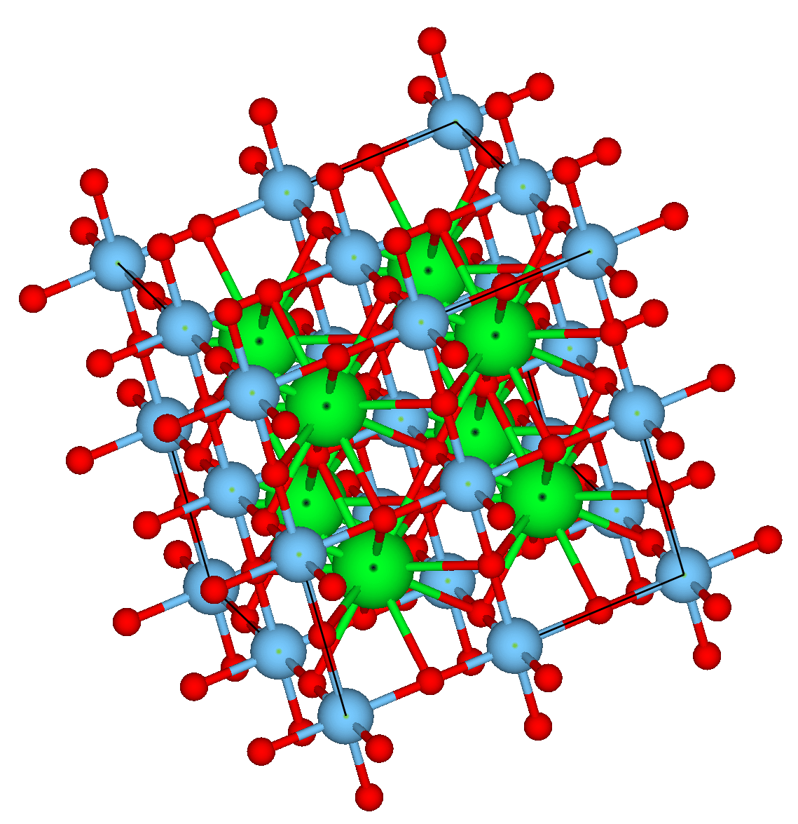
In this section we evaluate our algorithms via experimental simulations. We first focus on which we use as a benchmark. We do this because it is a well studied composition for which the Crystal Structure Prediction problem is solved. We have implemented the algorithms in Python 2.7 and we use the Atomic Simulation Environment (https://wiki.fysik.dtu.dk/ase/) package for setting up, manipulating, running, visualizing and analyzing atomistic simulations. All experiments were performed on a 4-core Intel i7-4710MQ with 8GB of RAM.
| Energy difference | ||||||
| k | ||||||
| atoms | ||||||
| atoms | ||||||
We evaluate the depth energy computation in several different dimensions. For all the experiments we performed for energy computation, we fixed the unit cell to be cubic. Firstly, we evaluate how depth energy computation behaves with respect to . We see that the method converges very fast and already achieves accuracy of three decimal points. Then, we compare our depth approach against GULP; see Table 1. Our goal is to provide an intuitively simpler to interpret and work with method for computing the energy. Even though the energy calculated by the depth approach differs from the one calculated by GULP, we observe that the relative energies between two random arrangements remain usually the same even for . To be more precise, let denote the energy of a feasible arrangement when and let denote the energy of this arrangement as it is computed by GULP. Our experiments show that if for two random feasible arrangements and it holds that , then for of 1000 pairs of arrangements. This percentage reaches for . For the “special” arrangement of ions that minimizes the energy computed by GULP, that is , our experiments show that it is always true that , for every , where is a random feasible structure over of them. So, this is a good indication that the arrangement that minimizes the energy for , also minimizes the energy overall. We view this as a striking result; it significantly simplifies the problem thus new, analytical, methods can be derived for the problem.
The next set of experiments compares the three neighborhoods described in Section 3 for 444The values of the Buckingham parameters can be found in the appendix. We compare them in several different dimensions: the average CPU time they need in order to find a local optimum with respect to their combinatorial neighborhood and the average drop in energy until they reach such a local optimum (Tables 2 and 4); the average CPU time the relaxation needs starting from such local minimum and the average drop in energy from relaxation (Tables 3 and 5). In addition, for the case of , we compare how often we can find the optimal arrangement from a single structure. We observe that the Axes neighborhood has the best tradeoff between energy drop and CPU time. The -ion-swap neighbourhood outperforms the other two in terms of running time, however it seems to decrease the probability of finding the best arrangement when performing a relaxation on the resulting structures. This renders the use of -ion-swap neighbourhood inappropriate. Axes neighborhood is significantly faster and performs smoother in terms of running time than the -swap neighbourhood. However the latter one performs better with respect to the energy drop, which is expected since axes is a subset of the 2-swap neighbourhood. In addition, the relaxation from the local minimum found by -swap significantly improves the probability of finding the best arrangement with only one relaxation. We should highlight that there exist structures where the relaxation cannot improve their energy, but the neighborhoods do; hence using Axes neighborhood we can escape from some local minima of the continuous space.
| Neighbourhood | Running time | Time stdev | Energy drop | Energy drop stdev |
| Axes | ||||
| -ion swap | ||||
| -swap |
| Neighbourhood | Running time | Time stdev | Energy drop | Energy drop stdev | Global minimum |
| Random structures-GULP | |||||
| Axes-GULP | |||||
| -ion swap-GULP | |||||
| -swap-GULP |
| Neighbourhood | Running time | Time stdev | Energy drop | Energy drop stdev |
| Axes | ||||
| -ion swap | ||||
| -swap |
| Neighbourhood | Running time | Time stdev | Energy drop | Energy drop stdev |
| Random structures-GULP | ||||
| Axes-GULP | ||||
| -ion swap-GULP | ||||
| -swap-GULP |
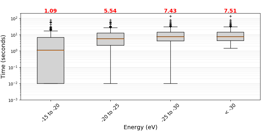
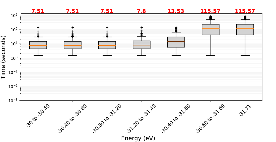
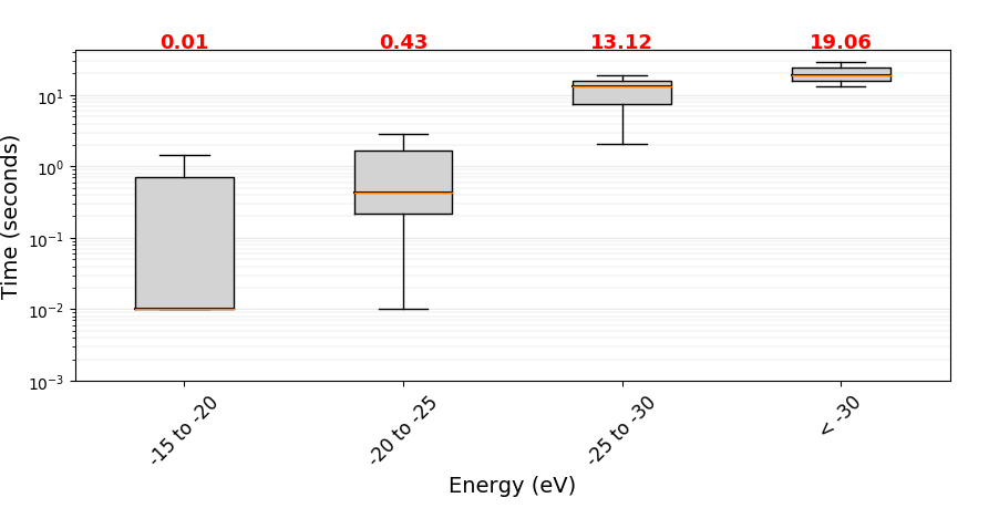
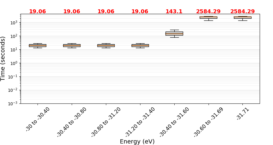
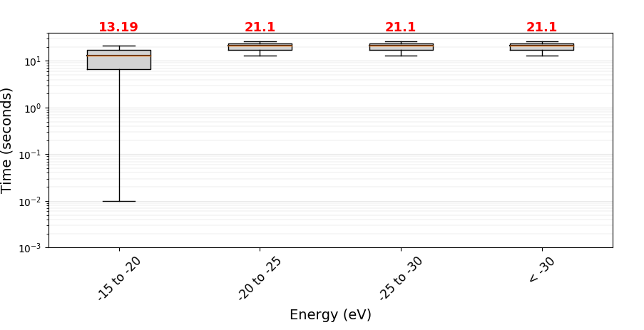
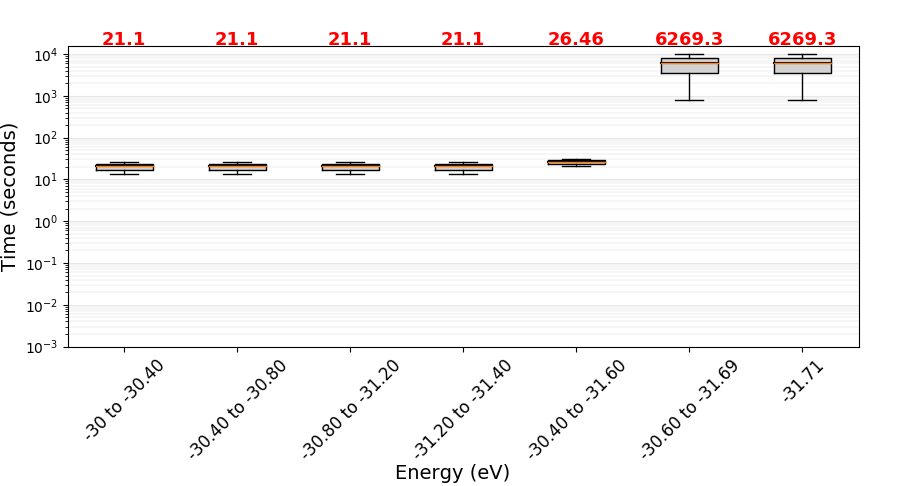
Next, we compare our algorithm for MinStructure against basin hopping where the next structure to relax is chosen at random. Based on the results of our previous experiments, we have chosen the Axes neighbourhood as an intermediate step before the relaxation. We have run these algorithms times for with atoms per unit cell, and times for with atoms per unit cell. We report how the energy varies with respect to time until the best arrangement is found (Fig. 2) and we report other statistics that further validate our approach (Table 6). As we can see, it is relatively easy to reach low levels of energy and the majority of time is needed to find the absolute minimum. In addition, the overhead posed by the use of the neighbourhood search divided by the time needed by the basin hopping to find the global minimum decreases as the number of the atoms in the unit cell increases.
| Algorithm | Number of atoms | Total time mean | Total time stdev | Relaxations | Time for relaxations | Time for local search |
| Axes-GULP | ||||||
| Basin hopping | ||||||
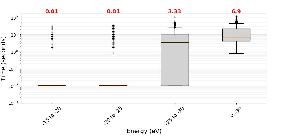
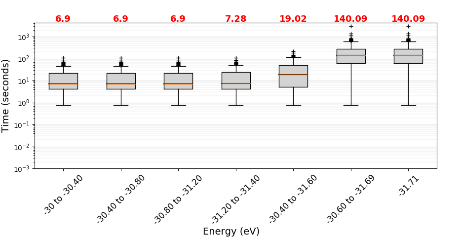
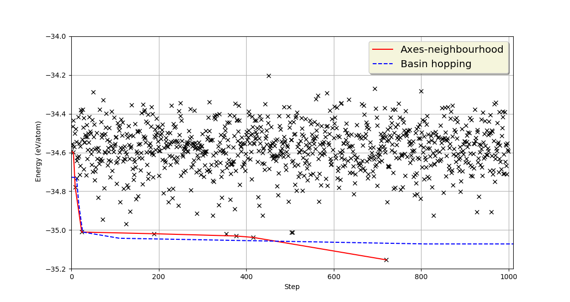
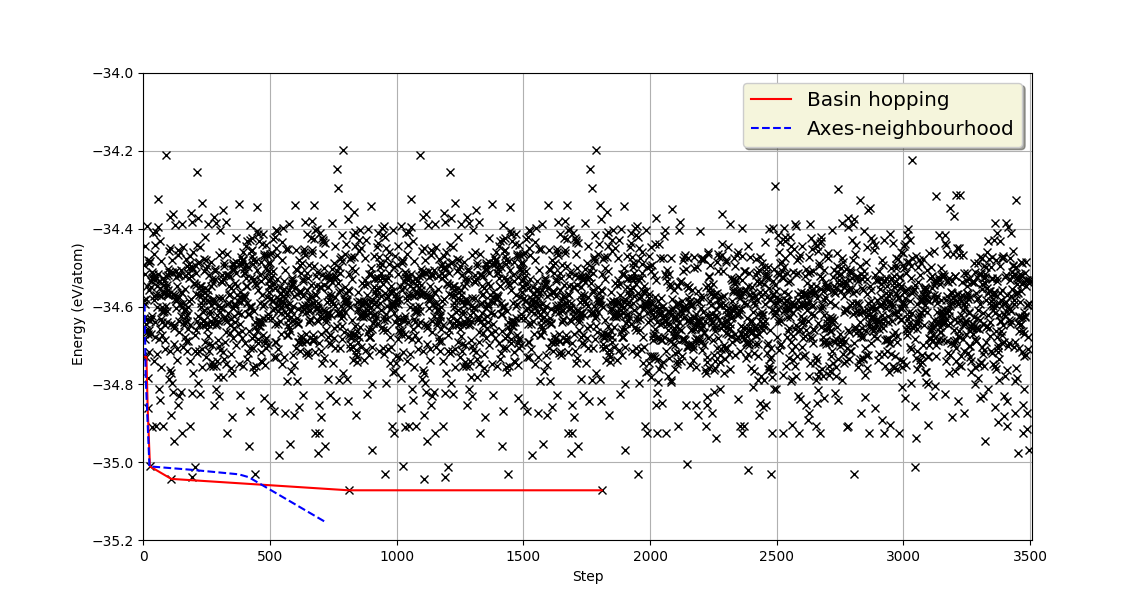
In our last set of experiments, we compare our algorithm against basin hopping algorithm for which contains atoms in its primitive unit cell. In this set of experiments, we produced random structures. We simulated basin hopping by sequentially relaxing the constructed structures. However, none of the relaxations managed to find the optimal configuration. Our algorithm, using the same order of structures as before, first used the Axes neighborhood as an intermediate step followed by a relaxation; it managed to find the optimal configuration after visiting only 720 structures (Fig. 3).
6 Conclusions
In this paper we have introduced and studied the Crystal Structure Prediction problem through the lens of computer science. This is an important and very exciting problem in computational chemistry, which computer scientists are not actively studying yet. We have identified several open questions whose solution would have significant impact to the discovery of new materials. These problems are challenging and several different techniques and machineries from computer science could be applied for solving them. Our simple-to-understand algorithms are a first step towards their solution. We hope that our algorithms will be used as benchmarks in the future, since more sophisticated techniques for basin hopping can be invented. For the energy computation via the depth approach, we conjecture that the arrangement that minimizes the energy for or , matches the arrangement that minimizes the energy when it is computed via GULP. Our numerical simulations provide significant evidence towards this. A formal result of this would greatly simplify the objective function of the optimization problem and it would give more hope to faster methods for relaxation. In addition, it could provide the foundations for new techniques for crystal structure prediction. Our algorithm that utilizes the Axes neighborhood as an intermediate step before relaxation, seems to speed up the time the standard basin hopping needs to find the global minimum. Are there any other neighborhoods that outperform the Axes one? Can local search, or Axes neighborhood in particular, improve existing methods for crystal structure prediction by a simple integration as an intermediate step? We believe that this is indeed the case.
References
- [1] D. Adamson, A. Deligkas, V. V. Gusev, and I. Potapov. On the hardness of energy minimisation for crystal structure prediction. In SOFSEM 2020: Theory and Practice of Computer Science - 46th International Conference on Current Trends in Theory and Practice of Informatics, SOFSEM 2020, Limassol, Cyprus, January 20-24, 2020, Proceedings, pages 587–596, 2020.
- [2] R. A. Buckingham. The classical equation of state of gaseous helium, neon and argon. Proceedings of the Royal Society of London. Series A. Mathematical and Physical Sciences, 168(933):264–283, 1938.
- [3] S. T. Call, D. Y. Zubarev, and A. I. Boldyrev. Global minimum structure searches via particle swarm optimization. Journal of computational chemistry, 28(7):1177–1186, 2007.
- [4] C. Collins, G. Darling, and M. Rosseinsky. The flexible unit structure engine (fuse) for probe structure-based composition prediction. Faraday discussions, 211:117–131, 2018.
- [5] C. Collins, M. Dyer, M. Pitcher, G. Whitehead, M. Zanella, P. Mandal, J. Claridge, G. Darling, and M. Rosseinsky. Accelerated discovery of two crystal structure types in a complex inorganic phase field. Nature, 546(7657):280, 2017.
- [6] S. Curtarolo, G. L. Hart, M. B. Nardelli, N. Mingo, S. Sanvito, and O. Levy. The high-throughput highway to computational materials design. Nature materials, 12(3):191, 2013.
- [7] D. M. Deaven and K.-M. Ho. Molecular geometry optimization with a genetic algorithm. Physical review letters, 75(2):288, 1995.
- [8] C. Freeman, J. Newsam, S. Levine, and C. Catlow. Inorganic crystal structure prediction using simplified potentials and experimental unit cells: application to the polymorphs of titanium dioxide. Journal of Materials Chemistry, 3(5):531–535, 1993.
- [9] J. D. Gale and A. L. Rohl. The general utility lattice program (gulp). Molecular Simulation, 29(5):291–341, 2003.
- [10] R. Gautier, X. Zhang, L. Hu, L. Yu, Y. Lin, T. O. Sunde, D. Chon, K. R. Poeppelmeier, and A. Zunger. Prediction and accelerated laboratory discovery of previously unknown 18-electron abx compounds. Nature chemistry, 7(4):308, 2015.
- [11] S. Goedecker. Minima hopping: An efficient search method for the global minimum of the potential energy surface of complex molecular systems. The Journal of chemical physics, 120(21):9911–9917, 2004.
- [12] G. Hautier, C. Fischer, V. Ehrlacher, A. Jain, and G. Ceder. Data mined ionic substitutions for the discovery of new compounds. Inorganic chemistry, 50(2):656–663, 2010.
- [13] D. C. Lonie and E. Zurek. Xtalopt: An open-source evolutionary algorithm for crystal structure prediction. Computer Physics Communications, 182(2):372–387, 2011.
- [14] N. Nosengo. Can artificial intelligence create the next wonder material? Nature News, 533(7601):22, 2016.
- [15] A. R. Oganov and C. W. Glass. Crystal structure prediction using ab initio evolutionary techniques: Principles and applications. The Journal of chemical physics, 124(24):244704, 2006.
- [16] A. R. Oganov, C. J. Pickard, Q. Zhu, and R. J. Needs. Structure prediction drives materials discovery. Nature Reviews Materials, page 1, 2019.
- [17] J. Pannetier, J. Bassas-Alsina, J. Rodriguez-Carvajal, and V. Caignaert. Prediction of crystal structures from crystal chemistry rules by simulated annealing. Nature, 346(6282):343, 1990.
- [18] C. J. Pickard. Real-space pairwise electrostatic summation in a uniform neutralizing background. Physical Review Materials, 2(1):013806, 2018.
- [19] C. J. Pickard and R. Needs. High-pressure phases of silane. Physical Review Letters, 97(4):045504, 2006.
- [20] C. J. Pickard and R. Needs. Ab initio random structure searching. Journal of Physics: Condensed Matter, 23(5):053201, 2011.
- [21] M. U. Schmidt and U. Englert. Prediction of crystal structures. Journal of the Chemical Society, Dalton Transactions, (10):2077–2082, 1996.
- [22] J. C. Schön. How can databases assist with the prediction of chemical compounds? Zeitschrift für anorganische und allgemeine Chemie, 640(14):2717–2726, 2014.
- [23] J. C. Schön and M. Jansen. First step towards planning of syntheses in solid-state chemistry: determination of promising structure candidates by global optimization. Angewandte Chemie International Edition in English, 35(12):1286–1304, 1996.
- [24] T. Siegrist and T. A. Vanderah. Combining magnets and dielectrics: Crystal chemistry in the bao- fe2o3- tio2 system. European Journal of Inorganic Chemistry, 2003(8):1483–1501, 2003.
- [25] T. Vanderah, J. Loezos, and R. Roth. Magnetic dielectric oxides: subsolidus phase relations in the bao: Fe2o3: Tio2system. Journal of Solid State Chemistry, 121(1):38–50, 1996.
- [26] P. Villars, K. Brandenburg, M. Berndt, S. LeClair, A. Jackson, Y.-H. Pao, B. Igelnik, M. Oxley, B. Bakshi, P. Chen, et al. Binary, ternary and quaternary compound former/nonformer prediction via mendeleev number. Journal of alloys and compounds, 317:26–38, 2001.
- [27] D. J. Wales and J. P. Doye. Global optimization by basin-hopping and the lowest energy structures of lennard-jones clusters containing up to 110 atoms. The Journal of Physical Chemistry A, 101(28):5111–5116, 1997.
- [28] J. D. Walker. Fundamentals of physics extended. Wiley, 2010.
- [29] Y. Wang, J. Lv, L. Zhu, and Y. Ma. Crystal structure prediction via particle-swarm optimization. Physical Review B, 82(9):094116, 2010.
Appendix A Appendix
| Interaction | (eV) | C (eV ) | |