Robust Q-learning

Abstract

Q-learning is a regression-based approach that is widely used to formalize the development of an optimal dynamic treatment strategy. Finite dimensional working models are typically used to estimate certain nuisance parameters, and misspecification of these working models can result in residual confounding and/or efficiency loss. We propose a robust Q-learning approach which allows estimating such nuisance parameters using data-adaptive techniques. We study the asymptotic behavior of our estimators and provide simulation studies that highlight the need for and usefulness of the proposed method in practice. We use the data from the “Extending Treatment Effectiveness of Naltrexone” multi-stage randomized trial to illustrate our proposed methods.

Keywords: Cross-fitting, Data-adaptive techniques, Dynamic treatment strategies, Residual confounding

1 Introduction

A dynamic treatment strategy is a sequence of decision rules that maps individual characteristics to a treatment option at each decision point (i.e., a specific point in time in which a treatment is to be considered or altered). An optimal dynamic treatment strategy seeks to make these decisions to maximize a particular expected health outcome (Lavori & Dawson, 2000; Murphy, 2005; Nahum-Shani et al., 2012a; Lei et al., 2012; Davidian et al., 2016). This is similar to clinical decision making whereby care providers tailor the type/dose of treatment over the course of clinical care based on ongoing information regarding patient progress in treatment.

The main goal of precision medicine (i.e., developing an effective dynamic treatment strategy) is to use patient characteristics to inform a personalized treatment plan as a sequence of decision rules that leads to the best possible health outcome for each patient (Nahum-Shani et al., 2012a; Chakraborty & Moodie, 2013; Moodie & Kosorok, 2015; Butler et al., 2018). Q-learning is a reinforcement learning algorithm that is widely used to estimate an optimal dynamic treatment strategy using data from multi-stage randomized clinical trials or observational studies (Watkins & Dayan, 1992; Nahum-Shani et al., 2012b; Laber et al., 2014). Starting with the final study stage, Q-learning finds the treatment option that optimizes the desired expected outcome. Fixing the optimally-chosen treatment at the final stage, Q-learning moves backward to the immediately preceding stage and searches for a treatment option assuming that future treatments will be optimized. The process continues until the first stage is reached. This backward induction procedure is designed to avoid treatment options that appear to be optimal in the short term but may lead to a less desirable long-term outcome (Chakraborty & Moodie, 2013; Davidian et al., 2016). Similar to other model-based approaches, model misspecification can seriously affect the result of Q-learning and the problem exacerbates substantially as the number of stages increases. Specifically, it can lead to residual confounding and suboptimal dynamic treatment strategies (Zhao et al., 2009; Ertefaie et al., 2016). An alternative approach is A-learning; this backward induction strategy is also model-based, hence subject to the possibility of misspecification, but imposes somewhat less restrictive regression model assumptions through modeling only the contrasts between treatments and the propensity of treatment assignment given the observed patient history (Murphy, 2003; Schulte et al., 2014; Shi et al., 2018). However, this extra robustness comes at the price substantially reduced efficiency; indeed, Q-learning may lead to a parameter estimate that can be up to 170% more efficient than A-learning (Schulte et al., 2014). Policy learning methods are another class of methods for estimating an optimal dynamic treatment regime that circumvent the need for the conditional outcome models by directly optimizing the expected outcome among a class of rules (Zhao et al., 2009, 2011, 2012; Song et al., 2015). Despite this appealing feature, policy learning methods are inefficient and fail to provide reasonable inference for the parameter estimates that define non-smooth decision rules (e.g., indicator or max operators) due to slow rates of convergence (Moodie & Kosorok, 2015; Zhao et al., 2015).

Doubly robust estimators that are based on modeling both the treatment and outcome processes have also been proposed for policy learning and for structural nested models (Zhang et al., 2012; Bai et al., 2013; Zhang et al., 2013; Wallace & Moodie, 2015). In general terms, consistency of the doubly robust estimators is guaranteed as long as either the treatment assignment mechanism or the postulated conditional mean outcome models are correctly specified, and semiparametric efficiency follows when both models are correctly specified (Rotnitzky et al., 1998; van der Laan & Robins, 2003; Tsiatis, 2007). However, while doubly robust estimators give two routes for consistent estimation, the performance of these estimators depends critically on the modeling choice for the indicated treatment and mean outcome parameters. In practice, finite-dimensional models are used that are too restrictive and likely to be misspecified (Wallace & Moodie, 2015). Kang et al. (2007) showed that doubly robust estimators can have poor performance when both models are misspecified. To mitigate this problem, bias reduction techniques have been proposed (Cao et al., 2009; Vermeulen & Vansteelandt, 2015, 2016). An alternative is to use flexible learning-based methods that may reduce the chance of inconsistency (Benkeser et al., 2017).

In this paper, we consider the problem of Q-learning for the setting of a two-stage dynamic binary treatment choice regime. A typical approach involves postulating linear models for both the first and second stage Q-functions that have stage-specific main effects involving pretreatment variables and interactions of these variables with the stage-specific treatment choice (e.g., Laber et al., 2014); however, only the interaction terms in these models directly influence the corresponding treatment decision functions that are optimized as part of the Q-learning process. Due to the nature of backward induction, the first stage model is likely to be a complicated function of the relevant covariates; misspecification of the main effect models in either stage can induce non-ignorable residual confounding. To increase robustness, we therefore consider the indicated main effects as unknown nuisance parameters and we adapt an approach originally proposed in Robinson (1988) for partial linear models that allows us to eliminate these parameters from the Q-functions. In particular, these hard-to-estimate parameters are replaced with models for the treatment assignment probability and mean outcome given pretreatment covariates that can be more easily estimated using, for example, nonparametric regression methods or related statistical learning methods (e.g., random forests). The resulting transformation process leads to consistent and asymptotically normal estimators of the so-called first- and second-stage blip functions that are robust to misspecification of the main effect nuisance parameters.

2 Notation and Formulation

Consider a two-stage study where binary treatment decisions are made at each time point. Let $\mathcal{O}=(\bm{X}_{1},A_{1},\bm{X}_{2},A_{2},Y)$ follow some probability distribution $P_{0}$ and suppose we observe $N$ independent, identically distributed trajectories of $\mathcal{O}.$ The vector $\bm{X}_{1}\in\mathcal{X}_{1}\subset\mathbbmss{R}^{p_{1}}$ consists of all available baseline covariates measured before treatment at the first decision point $A_{1}\in\{0,1\}$ and the vector $\bm{X}_{2}\in\mathcal{X}_{2}\subset\mathbbmss{R}^{p_{2}}$ consists of all available intermediate covariates measured before treatment at the second decision point $A_{2}\in\{0,1\}$. For notational convenience we define $\bm{S}^{0}_{i}=(\bm{X}_{1i}^{\top},A_{1i},\bm{X}_{2i}^{\top})^{\top}\in\mathcal{S}\subset\mathbbmss{R}^{p_{1}+p_{2}+1}$ and $\bm{W}^{0}_{i}=\bm{X}_{1i}\in\mathcal{X}_{1}\subset\mathbbmss{R}^{p_{1}}$. For later use, we also define variables $\bm{S}_{i}$ and $\bm{W}_{i},i=1,\ldots,n;$ respectively, each represents some finite dimensional function of the variables in $\bm{S}^{0}_{i}$ and $\bm{W}^{0}_{i}.$ Hence, knowledge of $\bm{S}^{0}_{i}$ and $\bm{W}^{0}_{i}$ respectively implies knowledge of $\bm{S}_{i}$ and $\bm{W}_{i};$ however, the reverse may not hold. The observed outcome $Y\in\mathbbmss{R}$ (measured after $A_{2}$) is assumed continuous, with a larger value of $Y$ indicating a better clinical outcome.

3 A Robust Formulation of Q-learning

The outcome $Y$ is assumed to satisfy the model

$$Y_{i}=\eta_{2}(\bm{S}^{0}_{i})+A_{2i}\cdot\Delta_{2}(\bm{S}^{0}_{i})+\epsilon_{2i},~{}\mathbbmss{E}(\epsilon_{2i}|\bm{S}^{0}_{i},A_{2i})=0,~{}i=1,\dotsc,N,$$ (1)

where the deterministic, unknown real-valued functions $\eta_{2}(\cdot)$ and $\Delta_{2}(\cdot)$ are defined on $\mathcal{S}.$ Because the treatment variable $A_{2}$ is binary, the additive error model (1) places no parametric constraints on the conditional mean function.

In Q-learning, backward induction is used to characterize the optimal dynamic treatment regime. Define the second stage Q-function

$$Q_{2}(\bm{s}^{0},a_{2})=\mathbbmss{E}(Y|\bm{S}^{0}=\bm{s}^{0},A_{2}=a_{2})=\eta_{2}(\bm{s}^{0})+a_{2}\Delta_{2}(\bm{s}^{0});$$ (2)

this measures “quality” when treatment $a_{2}$ is assigned to a patient with characteristics $\bm{s}^{0}$ at the second stage (Laber et al., 2014). Similarly, define the first stage Q-function as

$$Q_{1}(\bm{w}^{0},a_{1})=\mathbbmss{E}\bigl{\{}\max_{a_{2}}Q_{2}(\bm{S}^{0},a_{2})|\bm{W}^{0}=\bm{w}^{0},A_{1}=a_{1}\bigr{\}}$$ (3)

where, for $a_{2}\in\{0,1\}$,

$$\max_{a_{2}}Q_{2}(\bm{s}^{0},a_{2})=\eta_{2}(\bm{s}^{0})+\Delta_{2}(\bm{s}^{0})I\{\Delta_{2}(\bm{s}^{0})>0\}.$$

Analogously to $Q_{2}(\bm{s}^{0},a_{2}),$ $Q_{1}(\bm{w}^{0},a_{1})$ measures “quality” when treatment $a_{1}$ is assigned to a patient with characteristics $\bm{w}^{0}$ at baseline, assuming the optimal treatment choice is also made in the second stage. Because $A_{1}$ is binary, $Q_{1}(\bm{w}^{0},a_{1})$ can without loss of generality be written as $\eta_{1}(\bm{w}^{0})+a_{1}\Delta_{1}(\bm{w}^{0}),$ where the real-valued functions $\eta_{1}(\cdot)$ and $\Delta_{1}(\cdot)$ are defined on $\mathcal{X}_{1}.$ It then follows that

$$\max_{a_{1}}Q_{1}(\bm{w}^{0},a_{1})=\eta_{1}(\bm{w}^{0})+\Delta_{1}(\bm{w}^{0})I\{\Delta_{1}(\bm{w}^{0})>0\}.$$

Taken together, the optimal dynamic treatment regime is given by $d^{opt}(\bm{s}^{0})=\{d^{opt}_{1}(\bm{w}^{0}),d^{opt}_{2}(\bm{s}^{0})\}$, where $d^{opt}_{1}(\bm{w}^{0})=I\{\Delta_{1}(\bm{w}^{0})>0\}$ and $d^{opt}_{2}(\bm{s}^{0})=I\{\Delta_{2}(\bm{s}^{0})>0\}$. We note that, under standard causal assumptions and formulated appropriately, $\Delta_{1}(\bm{w}^{0})$ and $\Delta_{2}(\bm{s}^{0})$ are commonly referred to as the first and second stage blip functions.

A widely used convention in the literature on dynamic treatment regimes is to respectively model $Q_{2}(\bm{s}^{0},a_{2};\bm{b}_{2})=\bm{b}^{\top}_{20}\bm{s}_{20}+a_{2}\bm{b}^{\top}_{21}\bm{s}_{21}$ and $Q_{1}(\bm{w}^{0},a_{1};\bm{b}_{1})=\bm{b}^{\top}_{10}\bm{w}_{10}+a_{1}\bm{b}^{\top}_{11}\bm{w}_{11},$ where $\bm{s}_{2k},k=0,1$ are sets of variables derived from $\bm{s}^{0}$ (i.e., a realization of $\bm{S}^{0}$) and $\bm{w}_{1k},k=0,1$ are sets of variables derived from $\bm{w}^{0}$ (i.e., a realization of $\bm{W}^{0}$). These model formulations impose restrictive assumptions on both $\eta_{j}(\cdot)$ and $\Delta_{j}(\cdot),j=1,2$. However, the decision functions of interest only depend on the $\Delta_{j}(\cdot),j=1,2,$ or per the indicated linear models, on the $\bm{b}_{j1}s.$ Because misspecification of the models for the nuisance parameters $\eta_{j}(\cdot),j=1,2$ can induce residual confounding and affect the causal interpretation of the interaction terms, we propose a novel modification of the Q-learning approach that eliminates the need to directly model $\eta_{j}(\cdot),j=1,2.$ In particular, we adapt techniques originally introduced by Robinson (1988) for root-n consistent inference in semiparametric regression models, specifically partially linear models, to the Q-learning problem.

3.1 Regression model for Stage 2 decision function

Define $\mu_{2Y}(\bm{s}^{0})=\mathbbmss{E}(Y|\bm{S}^{0}=\bm{s}^{0})$ and $\mu_{2A}(\bm{s}^{0})=\mathbbmss{E}(A_{2}|\bm{S}^{0}=\bm{s}^{0});$ for now, we will proceed as if these two functions are known. Under (1), or equivalently (2), $\mu_{2Y}(\bm{s}^{0})=\eta_{2}(\bm{s}^{0})+\mu_{2A}(\bm{s}^{0})\Delta_{2}(\bm{s}^{0}),$ implying that

$$Y_{i}-\mu_{2Y}(\bm{S}^{0}_{i})=\{A_{2i}-\mu_{2A}(\bm{S}^{0}_{i})\}\cdot\Delta_{2}(\bm{S}^{0}_{i})+\epsilon_{2i},~{}\mathbbmss{E}(\epsilon_{2i}|\bm{S}^{0}_{i},A_{2i})=0,~{}i=1,\dotsc,N.$$ (4)

Define the centered second stage Q-function

$$Q_{2c}(\bm{s}^{0},a_{2})=\mathbbmss{E}\{Y-\mu_{2Y}(\bm{S}^{0})|\bm{S}^{0}=\bm{s}^{0},A_{2}=a_{2}\}=\{a_{2}-\mu_{2A}(\bm{s}^{0})\}\Delta_{2}(\bm{s}^{0});$$ (5)

observe that $Q_{2c}(\bm{s}^{0},a_{2})=Q_{2}(\bm{s}^{0},a_{2})-\mu_{2Y}(\bm{s}^{0}).$ Although $Q_{2c}(\bm{s}^{0},a_{2})$ differs from $Q_{2}(\bm{s}^{0},a_{2}),$ the action $a_{2}$ that maximizes $Q_{2c}(\bm{s}^{0},a_{2})$ is the same as that which maximizes $Q_{2}(\bm{s}^{0},a_{2})$ because $\mu_{2Y}(\bm{s}^{0})$ does not depend on the value of $a_{2}$. With $\eta_{2}(\bm{s}^{0})$ eliminated from $Q_{2c}(\bm{s}^{0},a_{2};\bm{\beta}_{2}),$ we propose to model (5) via

$$Q_{2c}(\bm{s}^{0},a_{2};\bm{\beta}_{2})=\{a_{2}-\mu_{2A}(\bm{s}^{0})\}\bm{s}^{\top}\bm{\beta}_{2},$$ (6)

where $\bm{s}$ denotes the realization of $\bm{S}$ (i.e., some finite set of variables derived from $\bm{S}^{0}$). Because

$$\mathbbmss{E}\left\{Y-\mu_{2Y}(\bm{S}^{0})-Q_{2c}(\bm{S}^{0},A_{2};\bm{\beta}_{2})|\bm{S}^{0}=\bm{s}^{0},A_{2}=a_{2}\right\}=\bigl{\{}a_{2}-\mu_{2A}(\bm{s}^{0})\bigr{\}}\bigl{\{}\Delta_{2}(\bm{s}^{0})-\bm{s}^{\top}\bm{\beta}_{2}\bigr{\}},$$

it is easily shown that

$$\bm{\beta}^{*}_{2} = \underset{\bm{\beta}_{2}}{\arg\!\min}~{}\mathbbmss{E}\left[\left\{Y-\mu_{2Y}(\bm{S}^{0})-Q_{2c}(\bm{S}^{0},A_{2};\bm{\beta}_{2})\right\}^{2}\right]$$

$$= \underset{\bm{\beta}_{2}}{\arg\!\min}~{}\mathbbmss{E}\left[\bigl{\{}A_{2}-\mu_{2A}(\bm{S}^{0})\bigr{\}}^{2}\bigl{\{}\Delta_{2}(\bm{S}^{0})-\bm{S}^{\top}\bm{\beta}_{2}\bigr{\}}^{2}\right].$$

The second expression shows that $\bm{S}^{\top}\bm{\beta}^{*}_{2}$ is the best (weighted) linear predictor of $\Delta_{2}(\bm{S}^{0}).$ For data $(Y_{i},\bm{S}^{0}_{i}),i=1,\ldots,N,$ the above developments further show that one can estimate $\bm{\beta}^{*}_{2}$ by $\tilde{\bm{\beta}}_{2N},$ calculated as the minimizer of

$$\sum_{i=1}^{N}\bigl{\{}Y_{i}-\mu_{2Y}(\bm{S}^{0}_{i})-Q_{2c}(\bm{S}^{0}_{i},A_{2i};\bm{\beta}_{2})\bigr{\}}^{2}.$$

Finally, maximizing $Q_{2c}(\bm{s}^{0},a_{2};\bm{\beta}^{*}_{2})$ for $a_{2}\in\{0,1\}$ gives $d^{opt}_{2}(\bm{s};\bm{\beta}^{*}_{2})=I\{\bm{s}^{\top}\bm{\beta}^{*}_{2}>0\}$ as the optimal model-based treatment decision in Stage 2, with a corresponding estimated decision rule of $\tilde{d}^{opt}_{2}(\bm{s})=I\{\bm{s}^{\top}\tilde{\bm{\beta}}_{2N}>0\}$ (i.e., assuming $\mu_{2Y}(\cdot)$ and $\mu_{2A}(\cdot)$ are known).

The calculations above evidently rely on the availability of $\mu_{2Y}(\cdot)$ and $\mu_{2A}(\cdot).$ The assumption that $\mu_{2Y}(\cdot)$ is known is particularly unrealistic; hence, in Section 4, we establish the properties of the corresponding least squares estimator when these functions are estimated from the available data using suitable consistent nonparametric estimators, such as those derived from random forests (e.g., Scornet et al., 2015) or Super Learner (van der Laan et al., 2007).

3.2 Regression model for Stage 1 decision function

By construction, the relevant first stage Q-function depends on the model for (2). Using the partially linear model of Section 3.1, the model-based analog of the second stage Q-function (2) is given by

$$Q_{2}(\bm{s}^{0},a_{2};\bm{\beta}^{*}_{2})=\mu_{2Y}(\bm{s}^{0})+Q_{2c}(\bm{s}^{0},a_{2};\bm{\beta}^{*}_{2}),$$ (7)

where the second term is defined in (6). In view of (3), we therefore re-define the first stage Q-function of interest as

$$Q_{1}(\bm{w}^{0},a_{1})=\mathbbmss{E}\bigl{\{}\max_{a_{2}}Q_{2}(\bm{S}^{0},a_{2};\bm{\beta}^{*}_{2})|\bm{W}^{0}=\bm{w}^{0},A_{1}=a_{1}\bigr{\}}.$$ (8)

Without loss of generality, and arguing similarly to the previous section, the fact that $A_{1}$ is binary means

$$Q_{1}(\bm{w}^{0},a_{1})=\eta_{1}(\bm{w}^{0})+a_{1}\Delta_{1}(\bm{w}^{0})$$ (9)

is a saturated nonparametric model for (8); here, $a_{1}\in\{0,1\}$ and the real-valued functions $\eta_{1}(\cdot)$ and $\Delta_{1}(\cdot)$ are defined on $\mathcal{X}_{1}$ and are not necessarily assumed to be the same functions that were initially used to define $Q_{1}(\bm{w}^{0},a_{1})$ a the beginning of Section 3.

Define

$$\tilde{Y}^{\dagger}=\max_{a_{2}}Q_{2}(\bm{S}^{0},a_{2};\bm{\beta}^{*}_{2});$$ (10)

then, it is not difficult to show that

$$\tilde{Y}^{\dagger} = \mu_{2Y}(\bm{S}^{0})+\bm{S}^{\top}\bm{\beta}^{*}_{2}\bigl{\{}I(\bm{S}^{\top}\bm{\beta}^{*}_{2}>0)-\mu_{2A}(\bm{S}^{0})\bigr{\}}.$$

Under (9), $\mathbbmss{E}\bigl{(}\tilde{Y}^{\dagger}\big{|}\bm{W}=\bm{w}^{0},A_{1}=a_{1}\bigr{)}=\eta_{1}(\bm{w}^{0})+a_{1}\Delta_{1}(\bm{w}^{0});$ similarly,

$$\mu_{1Y}(\bm{w}^{0})=\mathbbmss{E}\bigl{(}\tilde{Y}^{\dagger}\big{|}\bm{W}=\bm{w}^{0}\bigr{)}=\eta_{1}(\bm{w}^{0})+\mu_{1A}(\bm{w}^{0})\Delta_{1}(\bm{w}^{0}),$$

where $\mu_{1A}(\bm{w}^{0})=\mathbbmss{E}(A_{1}|\bm{W}=\bm{w}^{0}).$ Similarly to (5), we can write

$$Q_{1c}(\bm{w}^{0},a_{1})=\mathbbmss{E}\{\tilde{Y}^{\dagger}-\mu_{1Y}(\bm{W}^{0})|\bm{W}^{0}=\bm{w}^{0},A_{1}=a_{1}\}=\{a_{1}-\mu_{1A}(\bm{w}^{0})\}\Delta_{1}(\bm{w}^{0})$$ (11)

and, considering (6), can model (11) via

$$Q_{1c}(\bm{w}^{0},a_{1};\bm{\beta}_{1})=\{a_{1}-\mu_{1A}(\bm{w}^{0})\}\bm{w}^{\top}\bm{\beta}_{1},$$ (12)

where $\bm{w}$ is defined analogously to $\bm{s}$. Together, these results imply that

$$\mathbbmss{E}\left\{\tilde{Y}^{\dagger}-\mu_{1Y}(\bm{W}^{0})-Q_{1c}(\bm{W}^{0},A_{1};\bm{\beta}_{1})|\bm{W}^{0}=\bm{w}^{0},A_{1}=a_{1}\right\}=\bigl{\{}a_{1}-\mu_{1A}(\bm{w}^{0})\bigr{\}}\bigl{\{}\Delta_{1}(\bm{w}^{0})-\bm{w}^{\top}\bm{\beta}_{1}\bigr{\}}.$$

Similarly to the second stage problem, it now follows that

$$\bm{\beta}^{*}_{1} = \underset{\bm{\beta}_{1}}{\arg\!\min}~{}\mathbbmss{E}\left[\left\{\tilde{Y}^{\dagger}-\mu_{1Y}(\bm{W}^{0})-Q_{1c}(\bm{W}^{0},A_{1};\bm{\beta}_{1})\right\}^{2}\right]$$

$$= \underset{\bm{\beta}_{1}}{\arg\!\min}~{}\mathbbmss{E}\left[\bigl{\{}A_{1}-\mu_{1A}(\bm{W}^{0})\bigr{\}}^{2}\bigl{\{}\Delta_{1}(\bm{W}^{0})-\bm{W}^{\top}\bm{\beta}_{1}\bigr{\}}^{2}\right],$$

the latter implying that $\bm{W}^{\top}\bm{\beta}^{*}_{1}$ is the best (weighted) linear predictor of $\Delta_{1}(\bm{W}^{0}).$ For data $(Y_{i},\bm{S}^{0}_{i}),i=1,\ldots,N,$ and assuming that $\bm{\beta}^{*}_{2},$ $\mu_{jY}(\cdot)$ and $\mu_{jA}(\cdot),j=1,2$ are all known, the above developments further imply that one can estimate $\bm{\beta}^{*}_{1}$ using

$$\tilde{\bm{\beta}}_{1N}=\underset{\bm{\beta}_{1}}{\arg\!\min}\sum_{i=1}^{N}\bigl{\{}\tilde{Y}^{\dagger}_{i}-\mu_{1Y}(\bm{W}^{0}_{i})-Q_{1c}(\bm{W}^{0}_{i},A_{1i};\bm{\beta}_{1})\bigr{\}}^{2}.$$

Parallel to the second stage problem, the optimal model-based treatment decision in Stage 1, assuming the optimal model-based treatment is also given in Stage 2, would be $d^{opt}_{1}(\bm{w};\bm{\beta}^{*}_{1})=I\{\bm{w}^{\top}\bm{\beta}^{*}_{1}>0\}$, and may be estimated by $\tilde{d}^{opt}_{1}(\bm{w})=I\{\bm{w}^{\top}\tilde{\bm{\beta}}_{1N}>0\}$.

Of course, none of $\bm{\beta}^{*}_{2},$ $\mu_{jY}(\cdot)$ and possibly $\mu_{jA}(\cdot),j=1,2$ are known in practice; in Section 4, we establish the properties of the corresponding least squares estimator when these quantities are all estimated.

Remark: As an alternative to (10), one can substitute

$$\tilde{Y}=Y+\bm{S}^{\top}\bm{\beta}^{*}_{2}\bigl{\{}I(\bm{S}^{\top}\bm{\beta}^{*}_{2}>0)-A_{2}\bigr{\}}$$ (13)

for (10) when calculating $\tilde{\bm{\beta}}_{1N};$ this follows directly from the equalities $\mathbbmss{E}(\tilde{Y}|\bm{W}^{0}=\bm{w}^{0},A_{1}=a_{1})=\mathbbmss{E}(\tilde{Y}^{\dagger}|\bm{W}^{0}=\bm{w}^{0},A_{1}=a_{1})$ and $\mathbbmss{E}(\tilde{Y}|\bm{W}^{0}=\bm{w}^{0})=\mathbbmss{E}(\tilde{Y}^{\dagger}|\bm{W}^{0}=\bm{w}^{0}).$ $\Box$

4 Robust Q-learning: estimation in practice and corresponding theory

The two-stage procedure described in the previous section leads to a class of decision rules indexed by finite-dimensional parameter vectors, that is, $d^{opt}_{1}(\bm{W};\bm{\beta}_{1})=I(\bm{W}^{\top}\bm{\beta}_{1}>0)$ and $d^{opt}_{1}(\bm{S};\bm{\beta}_{2})=I(\bm{S}^{\top}\bm{\beta}_{2}>0)$ (e.g., Chakraborty & Moodie, 2013). Although not explicit in prior developments, the variable sets $\bm{S}$ and $\bm{W}$ are each assumed to contain a column of ones, so that the main effects of treatment at each stage can be included as part of the decision rule. The proposed approach eliminates the nuisance parameters $\eta_{j}(\cdot),j=1,2$ from the first and the second stage decision rules at the expense of introducing the four additional unknown functions $\mu_{jY}(\cdot)$ and $\mu_{jA}(\cdot),j=1,2.$ The advantage of the proposed approach is that the indicated functions depend on observables and can be easily estimated using any nonparametric regression or statistical learning method having sufficiently good prediction performance. Importantly, in the case of a sequentially randomized clinical trial, the functions $\mu_{jA}(\cdot),j=1,2$ are known and correct models are easily formulated.

4.1 Estimation in practice

The developments in the next two subsections assume that the original sample, with $N$ elements independently and identically distributed as $P_{0},$ has been randomly split into two disjoint and independent samples, say $\bm{D}_{I_{n}}$ and $\bm{D}_{I^{c}_{n}},$ with $n=O(N)$ (e.g., $n=N/2$) and where $\bm{I}_{n}$ and its complement $\bm{I}^{c}_{n}$ form a partition of the index set $\{1,\ldots,N\}$. The induced nuisance parameters $\hat{\mu}_{2Y}(\cdot),$ $\hat{\mu}_{2A}(\cdot),$ $\hat{\mu}_{1Y}(\cdot),$ and $\hat{\mu}_{1A}(\cdot)$ are to be estimated as described earlier using the data in $\bm{D}_{I^{c}_{n}};$ the finite dimensional parameters of interest are then estimated using the data $\bm{D}_{I_{n}},$ treating $\hat{\mu}_{2Y}(\cdot),$ $\hat{\mu}_{2A}(\cdot),$ $\hat{\mu}_{1Y}(\cdot),$ and $\hat{\mu}_{1A}(\cdot)$ as known functions. As described above, the use of such sample-splitting is a particularly simple form of cross-fitting and can be generalized easily (Chernozhukov et al., 2018); our use of sample splitting as described above will be sufficient to establish the main ideas for both estimation and asymptotics without unnecessarily complicating notation. Generalization to cross-fitting is straightforward and will be discussed at the end of Section 4.

Let $\hat{\mu}_{2Y}(\cdot)$, $\hat{\mu}_{1Y}(\cdot)$, $\hat{\mu}_{2A}(\cdot)$, and $\hat{\mu}_{1A}(\cdot)$ denote suitable estimates of $\mu_{jY}(\cdot)$ and $\mu_{jA}(\cdot),j=1,2$ derived from the data in $\bm{D}_{I^{c}_{n}}.$ Backward induction, implemented as described earlier with obvious modifications, can be used estimate the optimal dynamic treatment regime. In particular, for the second stage, we compute

$$\hat{\bm{\beta}}_{2n}=\underset{\bm{\beta}_{2}}{\arg\!\min}~{}\sum_{i\in\bm{I}_{n}}\left[Y_{i}-\hat{\mu}_{2Y}(\bm{S}^{0}_{i})-\{A_{2i}-\hat{\mu}_{2A}(\bm{S}^{0}_{i})\}\cdot\bm{S}_{i}^{\top}\bm{\beta}_{2}\right]^{2}.$$ (14)

To estimate the first stage parameters, we first calculate the estimated first stage pseudo-outcome

$$\hat{\tilde{Y}}_{i}=Y_{i}+\bm{S}_{i}^{\top}\hat{\bm{\beta}}_{2n}\{I(\bm{S}_{i}^{\top}\hat{\bm{\beta}}_{2n}>0)-A_{2i}\};$$ (15)

and then compute

$$\hat{\bm{\beta}}_{1n}=\underset{\bm{\beta}_{1}}{\arg\!\min}~{}\sum_{i\in\bm{I}_{n}}\left[\hat{\tilde{Y_{i}}}-\hat{\mu}_{1Y}(\bm{W}^{0}_{i})-\{A_{1i}-\hat{\mu}_{1A}(\bm{W}^{0}_{i})\}\cdot\bm{W}_{i}^{\top}\bm{\beta}_{1}\right]^{2}.$$ (16)

The notation in (14) and (16) emphasizes the fact that the nuisance parameters $\mu_{2Y}(\cdot),$ $\mu_{2A}(\cdot),$ $\mu_{1Y}(\cdot),$ and $\mu_{1A}(\cdot)$ are estimated using the outcome and full set of either second and first stage covariates, whereas the linear specifications used for modeling the centered Q-functions might not use all available covariate information.

As defined, the pseudo-outcomes are non-smooth functions of the data, hence so is $\hat{\bm{\beta}}_{1n}$; this can cause non-regularity problems for $\hat{\bm{\beta}}_{1n}$ (Laber et al., 2014). In particular, when $Pr(|\bm{S}^{\top}\bm{\beta}^{*}_{2}|=0)>0,$ i.e., there exists a strata of the covariates $\bm{S}$ used to model the Q-function that occurs with positive probability and for which treatment is neither beneficial nor harmful, the estimators of first stage regression coefficients become non-regular due to the non-differentiability of the indicator function in the definition of the pseudo-outcome.

The proposed Q-learning models essentially utilize the propensity score regression approach of Robins et al. (1992) to eliminate the problem of mismodeling hard-to-estimate infinite-dimensional parameters (i.e., $\eta_{j}(\cdot),j=1,2$) on the estimators of the $\bm{\beta}^{*}_{j}$s. The resulting estimator of $\bm{\beta}^{*}_{j}$ is consistent and asymptotically normal under suitable conditions on $\hat{\mu}_{jA}(.)$ and $\hat{\mu}_{jY}(.)$, $j=1,2$. In particular, the estimate of $\bm{\beta}^{*}_{j}$ is robust to misspecification of $\mu_{jY}(\cdot)$ provided that $\mu_{jA}(\cdot)$ is consistently estimated where $\bm{\beta}^{*}_{j}$ represents the parameters of the best linear approximation of the unknown $\Delta_{j}(\cdot).$ In practice, we recommend using ensemble learning methods such as Super Learner (van der Laan et al., 2007) for estimating both $\mu_{jA}(\cdot)$ and $\mu_{jY}(\cdot)$. Asymptotically, Super Learner performs as well as the best convex combination of the base learners in the chosen library, in the sense of minimizing the difference in risk compared to the corresponding oracle estimator. Moreover, the size of the library can grow at a polynomial rate compared with the sample size without affecting its oracle performance (van der Laan & Dudoit, 2003; Dudoit & van der Laan, 2003; van der Vaart et al., 2006). For these reasons, it is recommended that the library consist of a large and diverse set of regression modeling procedures (i.e., nonparametric, semiparametric, parametric). Importantly, these theoretical results only imply that Super Learner can match the performance of the (unknown) best possible convex combination of choices in the specified library. Thus, consistency is not guaranteed unless the corresponding oracle estimator is consistent and converges sufficiently fast. However, with the use of a sufficiently flexible library, Super Learner clearly improves one’s ability to construct a consistent estimator because it eliminates the need to select and subsequently rely on a single method of estimation.

4.2 Theoretical results

To further simplify notation, let $\Delta_{2i}=\Delta_{2}(\bm{S}^{0}_{i}),$ $\Delta_{1i}=\Delta_{1}(\bm{W}^{0}_{i}),$ $\mu_{2Ai}=\mu_{2A}(\bm{S}^{0}_{i}),$ $\hat{\mu}_{2Ai}=\hat{\mu}_{2A}(\bm{S}^{0}_{i}),$ $\mu_{1Ai}=\mu_{1A}(\bm{W}^{0}_{i}),$ and $\hat{\mu}_{1Ai}=\hat{\mu}_{1A}(\bm{W}^{0}_{i}).$ In addition, with $\bm{x}^{\otimes 2}=\bm{x}\bm{x}^{\top}$ for any vector $\bm{x},$ define the matrices

$$\mathbf{V}_{2n}=\frac{1}{n}\sum_{i\in\bm{I}_{n}}(A_{2i}-\mu_{2Ai})^{2}\bm{S}^{\otimes 2}_{i}~{}\mbox{ and }~{}\hat{\mathbf{V}}_{2n}=\frac{1}{n}\sum_{i\in\bm{I}_{n}}(A_{2i}-\hat{\mu}_{2Ai})^{2}\bm{S}^{\otimes 2}_{i}$$

$$\mathbf{V}_{1n}=\frac{1}{n}\sum_{i\in\bm{I}_{n}}(A_{1i}-\hat{\mu}_{1Ai})^{2}\bm{W}^{\otimes 2}_{i}~{}\mbox{ and }~{}\hat{\mathbf{V}}_{1n}=\frac{1}{n}\sum_{i\in\bm{I}_{n}}(A_{1i}-\hat{\mu}_{1Ai})^{2}\bm{W}^{\otimes 2}_{i}.$$

Let $\|\bm{x}\|_{q}$ denote the usual Q- norm of a vector $\bm{x}$ for $q=1,2,\infty$. Also, for $Z\sim P$ for some probability measure $P,$ suppose $f(\cdot)$ is any real-valued, $P-$measurable function; then, we define the $L^{2}(P)$ norm of $f(\cdot)$ as $\|f(Z)\|_{P,2}=\{\int\!f(\omega)^{2}dP(\omega)\}^{1/2}.$ For a real-valued function $h(\bm{s}^{0};\bm{D}_{I^{c}_{n}})$ defined for $\bm{s}^{0}\in\mathcal{S}$ whose calculation may depend on the data contained in $\bm{D}_{I^{c}_{n}},$ we can also define the random norm $\left\|h(\bm{S}^{0};\bm{D}_{I^{c}_{n}})\right\|_{P_{0},2}$ as the square-root of

$$\left\|h(\bm{S}^{0};\bm{D}_{I^{c}_{n}})\right\|^{2}_{P_{0},2}=\mathbbmss{E}\left\{\left\|h(\bm{S}^{0})\right\|^{2}_{\mathbb{P}_{n},2}\big{|}\bm{D}_{I^{c}_{n}}\right\},$$ (17)

where $\mathbb{P}_{n}$ denotes the empirical measure on $\bm{D}_{I_{n}}.$

Our results are established under the following assumptions.

Assumption 1.

(i) The support of $\bm{W}^{0}$ and the conditional treatment effect $\Delta_{1}(\bm{W}^{0})$ are uniformly bounded; (ii) the support of $\bm{S}^{0}$ and the conditional treatment effect $\Delta_{2}(\bm{S}^{0})$ are uniformly bounded; and, the supports of $\bm{S}$ and $\bm{W}$ are uniformly bounded.

Assumption 2.

(i) $\left\|\hat{\mu}_{1A}(\bm{W}^{0};\bm{D}_{I^{c}_{n}})-\mu_{1A}(\bm{W}^{0})\right\|^{2}_{P_{0},2}=o_{p}(n^{-1/2});$ (ii) $\left\|\hat{\mu}_{2A}(\bm{S}^{0};\bm{D}_{I^{c}_{n}})-\mu_{2A}(\bm{S}^{0})\right\|^{2}_{P_{0},2}=o_{p}(n^{-1/2}).$

Assumption 3.

(i) $\left\|\hat{\mu}_{1Y}(\bm{W}^{0};\bm{D}_{I^{c}_{n}})-\mu_{1Y}(\bm{W}^{0})\right\|^{2}_{P_{0},2}=o_{p}(1);$ (ii) $\left\|\hat{\mu}_{2Y}(\bm{S}^{0};\bm{D}_{I^{c}_{n}})-\mu_{2Y}(\bm{S}^{0})\right\|^{2}_{P_{0},2}=o_{p}(1).$

Assumption 4.

(i) $\left\|\hat{\mu}_{1Y}(\bm{W}^{0};\bm{D}_{I^{c}_{n}})-\mu_{1Y}(\bm{W}^{0})\right\|_{P_{0},2}\left\|\hat{\mu}_{1A}(\bm{W}^{0};\bm{D}_{I^{c}_{n}})-\mu_{1A}(\bm{W}^{0})\right\|_{P_{0},2}=o_{p}(n^{-1/2});$
(ii) $\left\|\hat{\mu}_{2Y}(\bm{S}^{0};\bm{D}_{I^{c}_{n}})-\mu_{2Y}(\bm{S}^{0})\right\|_{P_{0},2}\left\|\hat{\mu}_{2A}(\bm{S}^{0};\bm{D}_{I^{c}_{n}})-\mu_{2A}(\bm{S}^{0})\right\|_{P_{0},2}=o_{p}(n^{-1/2})$

Assumption 5.

There exists $1\leq n_{0}<\infty$ such that $\mathbf{V}_{jn}$ and $\hat{\mathbf{V}}_{jn},j=1,2$ are positive definite for $n\geq n_{0}$.

Assumption 6.

$P\big{(}|\bm{S}_{1}^{\top}\bm{\beta}^{*}_{2}|=0\big{)}=0.$

Assumption 7 requires no discussion. Assumptions 8 - 10 impose reasonable conditions on the estimators of the nuisance parameters estimated using cross fitting that are satisified by many machine learning algorithms; see Chernozhukov et al. (2018) for further discussion. Assumption 11 imposes reasonable conditions on the existence and uniqueness of the least squares estimators (14) and (16). Assumption 11 combined with independent, identically distributed sampling ensures that the limiting matrices

$$\mathbf{V}_{2}=\mathbbmss{E}\left\{\mbox{var}\left(A_{2}|\bm{S}^{0}\right)\bm{S}^{\otimes 2}\right\}~{}\mbox{ and }~{}\mathbf{V}_{1}=\mathbbmss{E}\left\{\mbox{var}\left(A_{1}|\bm{W}^{0}\right)\bm{W}^{\otimes 2}\right\}$$

both exist and are positive definite. Finally, Assumption 12 is imposed to avoid non-regular asymptotic behavior in the first stage least squares estimator (16). Inferences for the parameters that define the estimated optimal dynamic treatment regime $\hat{d}^{opt}_{2}(\bm{s})=I\{\bm{s}^{\top}\hat{\bm{\beta}}_{2n}>0\}$ and $\hat{d}^{opt}_{1}(\bm{w})=I\{\bm{w}^{\top}\hat{\bm{\beta}}_{1n}>0\}$ can now be derived using the results in the following theorem.

Theorem 1.

Suppose that Assumptions 7 - 12 hold.

• Let $\hat{\bm{\beta}}_{2n}$ be given by (14). Then, $\sqrt{n}(\hat{\bm{\beta}}_{2n}-{\bm{\beta}}^{*}_{2})\stackrel{{\scriptstyle d}}{{\rightarrow}}N(\bm{0},\mathbf{V}^{-1}_{2}\mathbf{Q}_{2}\mathbf{V}^{-1}_{2})$ where the matrices $\mathbf{V}_{2}=\mathbbmss{E}\left\{\mbox{var}\left(A_{2}|\bm{S}^{0}\right)\bm{S}^{\otimes 2}\right\}$ and $\mathbf{Q}_{2}=\mathbbmss{E}(\bm{J}_{2}^{\otimes 2})$ for

  $$\bm{J}_{2}=\{A_{2}-\mu_{2A}(\bm{S}^{0})\}\bm{S}\left[Y-\mu_{2Y}(\bm{S}^{0})-\{A_{2}-\mu_{2A}(\bm{S}^{0})\}\bm{S}^{\top}{\bm{\beta}}^{*}_{2}\right].$$

• Let $\hat{\bm{\beta}}_{1n}$ be given by (16). Then, $\sqrt{n}(\hat{\bm{\beta}}_{1n}-{\bm{\beta}}^{*}_{1})\stackrel{{\scriptstyle d}}{{\rightarrow}}N(\bm{0},\mathbf{V}^{-1}_{1}\mathbf{Q}_{1}\mathbf{V}^{-1}_{1})$ where the matrices $\mathbf{V}_{1}=\mathbbmss{E}\left\{\mbox{var}\left(A_{1}|\bm{W}^{0}\right)\bm{W}^{\otimes 2}\right\}$ and $\mathbf{Q}_{1}=\mathbbmss{E}\{(\bm{J}_{1}+\bm{K}\mathbf{V}^{-1}_{2}\bm{J}_{2})^{\otimes 2}\}$ for

  $$\bm{J}_{1}=\{A_{1}-\mu_{1A}(\bm{W}^{0})\}\bm{W}\left[\tilde{Y}-\mu_{1A}(\bm{W}^{0})-\{A_{1}-\mu_{1A}(\bm{W}^{0})\}\bm{W}^{\top}{\bm{\beta}}^{*}_{1}\right]$$

  and

  $$\bm{K}=\mathbbmss{E}\big{[}\{A_{1}-\mu_{1A}(\bm{W}^{0})\}\{I(\bm{S}^{\top}\bm{\beta}^{*}_{2}>0)-A_{2}\}\bm{W}\bm{S}^{\top}\big{]}.$$

The following corollary to Theorem 1 shows that Assumption 12 is not required to establish the results in part (b) in certain settings, in contrast to the standard form of Q-learning.

Corollary 1.

Suppose Assumptions 7 - 11 hold. In addition, suppose $\mathbbmss{E}\left(A_{1i}-{\mu}_{1Ai}\mid\bm{W}_{i},\bm{S}_{i},\bm{I}_{n}\right)=0,i\in\bm{I}_{n}.$ Then, Theorem 1, part (b) remains true.

The set of variables $\bm{S}$ used for modeling the second stage decision rule are those thought to be potential effect modifiers for the second stage treatment assigment $A_{2};$ hence, a sufficient condition for the Corollary to hold is that $A_{1}$ is independent of $\bm{S}$, conditionally on the set of pre-treatment covariates $\bm{W}$ included in the first stage model. Note that this does not preclude the possibility that $A_{1}$ can affect variables in $\bm{S}^{0}$ that are not part of $\bm{S}.$ Due to the way in which $A_{1i}-{\mu}_{1Ai}$ enters the estimating equation of Wallace & Moodie (2015, Eqn. (4)), it is unclear whether their approach avoids non-regularity under the same conditions as Corollary 1 even when the propensity model $\mu_{1A}(\bm{W}^{0})$ has been correctly specified.

4.3 Generalization to cross-fitting

Sample splitting, as used in the previous two sections, does not make use of the full sample of $N$ observations to estimate the finite-dimensional regression parameters, and this can negatively impact efficiency. We now describe an alternative approach, cross-fitting, that uses the full sample to estimate the desired target parameters.

Suppose that $N=nK$ for some integer $n$ and some integer $K\geq 2.$ Using an extension of previous notation, we first randomly split the original sample into disjoint (hence independent) samples $(\bm{D}_{I_{n,k}})_{k=1}^{K}$ such that the size of each sample is $n=N/K$ and $\bm{I}_{n,k},k=1,\ldots,K$ partition the indices $\{1,\ldots,N\}.$ Analogously to before, define $\bm{I}_{n,k}^{c}$ as the set of sample indices that are not included in $\bm{I}_{n,k};$ that is, $\bm{I}_{n,k}^{c}=\{1,2,\cdots,N\}\setminus\bm{I}_{n,k},k=1,\ldots,K$. Then, for each $k=1,2,\cdots,K$, estimate the nuisance parameters $\mu_{2Y}(\cdot),$ $\mu_{2A}(\cdot),$ $\mu_{1Y}(\cdot),$ and $\mu_{1A}(\cdot)$ using the data in $\bm{D}_{I_{n,k}^{c}};$ we respectively denote these estimators $\hat{\mu}_{2Y}(\cdot;\bm{D}_{I_{n,k}^{c}}),$ $\hat{\mu}_{2A}(\cdot;\bm{D}_{I_{n,k}^{c}}),$ $\hat{\mu}_{1Y}(\cdot;\bm{D}_{I_{n,k}^{c}}),$ and $\hat{\mu}_{1A}(\cdot;\bm{D}_{I_{n,k}^{c}}),$ $k=1,\ldots K.$ Finally, we define

$$\hat{\bm{\beta}}_{2n}=\underset{\bm{\beta}_{2}}{\arg\!\min}~{}\sum_{k=1}^{K}\sum_{i\in\bm{I}_{n,k}}\left[Y_{i}-\hat{\mu}_{2Y}(\bm{S}^{0}_{i};\bm{D}_{I_{n,k}^{c}})-\{A_{2i}-\hat{\mu}_{2A}(\bm{S}^{0}_{i};\bm{D}_{I_{n,k}^{c}})\}\cdot\bm{S}_{i}^{\top}\bm{\beta}_{2}\right]^{2}$$ (18)

and

$$\hat{\bm{\beta}}_{1n}=\underset{\bm{\beta}_{1}}{\arg\!\min}~{}\sum_{k=1}^{K}\sum_{i\in\bm{I}_{n,k}}\left[\hat{\tilde{Y_{i}}}-\hat{\mu}_{1Y}(\bm{W}^{0}_{i};\bm{D}_{I_{n,k}^{c}})-\{A_{1i}-\hat{\mu}_{1A}(\bm{W}^{0}_{i};\bm{D}_{I_{n,k}^{c}})\}\cdot\bm{W}_{i}^{\top}\bm{\beta}_{1}\right]^{2}.$$ (19)

This form of cross-fitting essentially corresponds to “DML2” as described in Chernozhukov et al. (2018, Def. 3.2). Like sample splitting, cross-fitting helps to guarantee that some of the remainder terms in the asymptotic linearity expansion converge to zero at an appropriately fast rate. However, in contrast to sample splitting, cross-fitting as described above is also capable of asymptotically achieving the same efficiency as in the case where estimators of the regression parameters are computed using all $N$ observations (i.e., with $\mu_{jA}(\cdot)$ and $\mu_{jY}(\cdot)$ $j=1,2$ being known).

5 Simulation studies

We examined the performance of our proposed Q-learning method under different simulation scenarios with various functional complexities and degrees of non-regularity (i.e., violation of Assumption 12).

The main simulation in the regular setting uses the following data generation mechanism. Let $\bm{X}_{1}=(X_{11},X_{12},X_{13},X_{14},X_{15})^{\top}$ be a 5-dimensional vector of baseline covariates independently generated and uniformly distributed on [-0.5,0.5]. Let $\bm{X}_{2}=(X_{21},X_{22},X_{23},X_{24},X_{25})^{\top},$ $X_{2l}=X_{1l}+U_{l},~{}l=1,2,3;$ $X_{24}=0.35X_{15}+U_{4};$ and, $X_{25}=U_{5},$ where $U_{l},l=1,\ldots,5$ are independent and uniformly distributed on [-0.5,0.5]. It is assumed that only nonresponders to the first stage treatment will receive the second stage treatment. This nonresponse indicator $R$ equals 1 if $X_{24}$ is less than its median value and is 0 otherwise. Finally, the first and second stage treatments $A_{j}$ are generated from a Bernoulli distribution with success probability $\mu_{jA}(\cdot)=[1+\exp\{-\lambda_{jA}(\cdot)\}]^{-1}$, where $\lambda_{jA}(\cdot)$ depends on either $\bm{S}^{0}=(\bm{X}^{\top}_{1},A_{1},\bm{X}^{\top}_{2})^{\top}$ ($j$=2) or $\bm{W}^{0}=\bm{X}_{1}$ ($j$=1); see Section 5.1.

5.1 Performance: regular setting

In this case, we consider performance for models that satisfy Assumption 12. To implement our proposed method, we used the R package SuperLearner (Polley et al., 2019) to estimate $\mu_{1Y}(\cdot)$, $\mu_{2Y}(\cdot)$, $\mu_{1A}(\cdot)$, and $\mu_{2A}(\cdot)$. The library used for SuperLearner included generalized linear models (i.e., glm), generalized additive models (i.e., gam; Hastie, 2019), multivariate adaptive regression splines (i.e., earth; Milborrow, 2019), random forests (i.e., randomForest; Liaw & Wiener, 2002), and support vector machines (i.e., svm from the R package e1071; Meyer et al., 2019); estimation was implemented with all tuning parameters set to their respective default values. This simulation study uses four different functional forms for the treatment assignment model $\mu_{jA}(\cdot)=[1+\exp\{-\lambda_{jA}(\cdot)\}]^{-1}$, $j=1,2$:

• Randomized: $\lambda_{jA}(\cdot)=0$

• Linear: $\lambda_{jA}(\cdot)=2X_{j1}+2X_{j2}+X_{j3}+0.1X_{j4}+0.1X_{j5}$

• Quadratic: $\lambda_{jA}(\cdot)=1.4\{(X_{j1}-0.5)^{2}+(X_{j2}-0.5)^{2}+0.6(X_{j3}-0.5)^{2}+0.5(X_{j4}-0.5)^{2}+0.5(X_{j5}-0.5)^{2}+X_{j1}+X_{j2}+0.6X_{j3}+0.5X_{j4}+0.5X_{j5}-2\}$.

• InterQuad: $\lambda_{jA}(\cdot)=1.4\{(X_{j1}-0.5)^{2}+(X_{j2}-0.5)^{2}+0.6(X_{j3}-0.5)^{2}+0.5(X_{j4}-0.5)^{2}+0.5(X_{j5}-0.5)^{2}+X_{j1}+X_{j2}+0.6X_{j3}+0.5X_{j4}+0.5X_{j5}+X_{j1}X_{j2}-2\}.$

The Randomized model corresponds to a SMART-like trial where simple randomization is used at baseline and then simple re-randomization occurs among the set of non-responders at the first stage. The randomization model, part of the trial design, is therefore known and the inclusion of an appropriate glm model in the Super Learner library should ensure that $\mu_{jA}(\cdot)$ can be consistently estimated at the usual parametric rate. The other three settings are meant to correspond to increasingly complex observational data settings, where the “assignment” mechanism by which patients follow a particular treatment regimen is covariate-dependent, not randomized, and is not considered to be known by design. Hence, the analyst cannot knowingly select a correctly specified parametric model a priori. In the case of the Linear model, the inclusion of a glm model in the Super Learner library again ensures that $\mu_{jA}(\cdot)$ can be consistently estimated at the usual parametric rate. For the other two models, the inclusion of methods such as gam and randomForest will help to mitigate, but not necessarily eliminate, the possibility of inconsistent estimation. These observations highlight the importance of using flexible methods when modeling $\mu_{jA}(\cdot),j=1,2,$ particularly in observational data settings.

The outcome models are given by :

• Linear^R: $Y=\mathbf{X}_{1}^{\top}\bm{\alpha}_{1}+\mathbf{X}_{2}^{\top}\bm{\alpha}_{2}+A_{1}\mathbf{X}_{1}^{\top}\bm{\theta}_{1}+A_{2}R\mathbf{X}_{2}^{\top}\bm{\theta}_{2}+\epsilon$ where $\bm{\alpha}_{1}=\bm{\alpha}_{2}=(1,0.1,0.1,0.1,0.1)^{\top}$, $\bm{\theta}_{1}=(0,0,0,0,0)^{\top}$ and $\bm{\theta}_{2}=(1,1,0,0,0)^{\top}$;

• FGS^R: $Y=f(\mathbf{X}_{1})+f(\mathbf{X}_{2})+A_{1}\mathbf{X}_{1}^{\top}\bm{\theta}_{1}+A_{2}Rg(\mathbf{X}_{2})+\epsilon$ where $\bm{\theta}_{1}=(0,0,0,0,0)^{\top}$ and for $\bm{x}=(x_{1},x_{2},x_{3},x_{4},x_{5})^{\top},$ we set $g(\bm{x})=2\sin(\pi x_{1}x_{2})+2(x_{2}-0.5)^{2}$ and

  $$f(\bm{x})=-1.5+\sin(\pi x_{1}x_{2})+2(x_{3}-0.5)^{2}+x_{4}+1.5\frac{x_{1}}{|x_{2}|+|x_{3}|}+2x_{1}(x_{2}+x_{3}).$$

The noise variable $\epsilon$ is generated from $\mathrm{N}(0,\sigma=0.5)$.

In connecting the above Linear^R outcome model specification with earlier notation, we have $\bm{S}^{0}=(\bm{X}_{1}^{\top},A_{1},\bm{X}_{2}^{\top})^{\top}$, $\eta_{2}(\bm{S}^{0})=\mathbf{X}_{1}^{\top}\bm{\alpha}_{1}+\mathbf{X}_{2}^{\top}\bm{\alpha}_{2}+A_{1}\mathbf{X}_{1}^{\top}\bm{\theta}_{1}$ and $\Delta_{2}(\bm{S}^{0})=R\mathbf{X}_{2}^{\top}\bm{\theta}_{2},$ where $R$ is a function of $X_{24}$ only; we further have $\bm{W}^{0}=\bm{X}_{1}$. We respectively use $\bm{S}=R(1,X_{21},X_{22},X_{23})^{\top}$ and $\bm{W}=(1,X_{11},X_{12})^{\top}$ for modeling the relevant Q-functions. In this case, the target of estimation $\bm{\beta}^{*}_{2}=(0,\theta_{21},\theta_{22},\theta_{23})^{\top}$ and it can additionally be shown that (5) coincides with (6). However, for the FGS^R outcome model, $\eta_{2}(\bm{S}^{0})=f(\mathbf{X}_{1})+f(\mathbf{X}_{2})+A_{1}\mathbf{X}_{1}^{\top}\bm{\theta}_{1}$ and $\Delta_{2}(\bm{S}^{0})=Rg(\mathbf{X}_{2});$ here, (5) does not coincide with (6) since the linear parametric specification used in the latter is not equal to $\Delta_{2}(\bm{S}).$ In this case $\bm{S}^{\top}\bm{\beta}^{*}_{2}$ still exists as the best linear projection of $\Delta_{2}(\bm{S}^{0})$ on to the linear space spanned by $\bm{S};$ however, its value for this simulation study must be determined numerically (e.g., through simulation).

In general, it is not similarly straightforward to characterize the functions $\eta_{1}(\bm{W}^{0})$ and $\Delta_{1}(\bm{W}^{0}),$ or the value of $\bm{\beta}^{*}_{1}$ in the first stage models, without appealing to numerical methods. However, in the current simulation setting, the value of $\bm{\beta}^{*}_{1}$ can be determined exactly for both the Linear^R and FGS^R outcome model specifications. Specifically, neither model involves an interaction between $A_{1}$ and $A_{2}$; more generally, there is no correlation between $A_{1}$ and the second stage variables $A_{2}$ and $\mathbf{X}_{2}.$ As a result, the linear term $A_{1}\mathbf{X}_{1}^{\top}\bm{\theta}_{1}$ that appears in both the Linear^R and FGS^R outcome model specifications accurately describes the interaction between treatment $A_{1}$ and $\mathbf{X}_{1}$ in the true first stage Q-function (i.e., $\Delta_{1}(\bm{W}^{0})=\bm{W}^{\top}\bm{\theta}_{1}=\mathbf{X}_{1}^{\top}\bm{\theta}_{1}=\bm{0})$. It follows that $\bm{\beta}^{*}_{1}=\bm{0}$ and hence that expression (11) also coincides with (12).

Table 1: Performance of the proposed Q-learning method for estimating the second stage parameters under different model complexities. The true parameters for the linear and FGS outcome models are respectively $\beta^{*}_{2,1}=1$, $\beta^{*}_{2,2}=1$ and $\beta^{*}_{2,1}\approx 0$, $\beta^{*}_{2,2}\approx-2.$

	$\beta^{*}_{2,1}$						$\beta^{*}_{2,2}$
	QN,N		Proposed		dWOLSN,N		QN,N		Proposed		dWOLSN,N
Outcome	Bias	S.D.	Bias	S.D.	Bias	S.D.	Bias	S.D.	Bias	S.D.	Bias	S.D.
Randomized Treatment Assignment Model
LinearR	0.003	0.041	0.003	0.081	0.002	0.082	0.001	0.038	0.004	0.081	0.002	0.076
FGSR	0.041	0.404	0.005	0.514	0.024	0.763	0.002	0.241	0.037	0.211	0.031	0.377
Linear Treatment Assignment Model
LinearR	0.004	0.041	0.004	0.101	0.006	0.095	0.003	0.042	0.000	0.101	0.002	0.098
FGSR	2.500	0.368	0.060	0.662	0.050	0.886	2.527	0.238	0.064	0.365	0.055	0.526
Quadratic Treatment Assignment Model
LinearR	0.006	0.040	0.005	0.082	0.007	0.081	0.004	0.040	0.011	0.082	0.003	0.082
FGSR	0.797	0.419	0.093	0.586	0.811	0.827	0.012	0.247	0.017	0.276	0.022	0.409
InterQuad Treatment Assignment Model
LinearR	0.000	0.041	0.014	0.094	0.001	0.084	0.002	0.039	0.019	0.086	0.002	0.079
FGSR	0.749	0.470	0.070	0.612	0.758	0.916	0.442	0.234	0.019	0.271	0.455	0.402

In our main simulation study, there are 8 possible model combinations represented by the outcome and treatment assignment models, and within each setting we compare the performance of the proposed method for estimating $\bm{\beta}_{j}^{*},j=1,2$ to the standard form of Q-learning (Q_N,N) and also to the weighted least squares (dWOLS_N,N) estimator proposed by Wallace & Moodie (2015). The subscripts on these latter two estimators denote the fact that standard errors would normally be calculated using the $N$-out-of-$N$ bootstrap (i.e., in the regular setting). In the case of dWOLS${}_{N,N},$ linear models are used for the relevant Q-function model specification and logistic regression models are used for estimating the treatment assignment probabilities. The estimation of $\bm{\beta}_{j}^{*},j=1,2$ is not subject to residual confounding bias for any of the proposed methods under the Linear^R outcome model specification. However, there is a possibility of such bias under the FGS^R in the case of Q_N,N and dWOLS_N,N. To be more specific, residual confounding bias under the FGS^R outcome model is expected for Q_N,N regardless of the treatment assignment model. For dWOLS_N,N, the Randomized and Linear first and second stage treatment assignment models are correctly specified and easily modeled. Hence, under the FGS^R outcome model specification, a significant potential for bias arises only under the Quadratic or InterQuad treatment assignment rules. For the proposed method, residual confounding bias when estimating $\bm{\beta}_{j}^{*}$ is not anticipated provided that $\mu_{jA}(\cdot),j=1,2$ are sufficiently well-estimated.

We generate 500 datasets of size 2000 to examine the performance of our proposed method and use cross-fitting as described in Section 4.3 with $K=2$ to estimate the desired target parameters. Tables 1 and 2 show the empirical absolute bias and standard deviations of the second and first stage parameter estimates (i.e., standard errors). The values of $\beta^{*}_{2,1}\approx 0$ and $\beta^{*}_{2,2}\approx-2$ are determined by simulation. As expected, standard Q-learning performs poorly except under the Randomized treatment assignment model. The proposed method and dWOLS_N,N also perform similarly well under the Randomized and Linear treatment assignment models for estimating the first and second stage parameters. However, under the FGS^R outcome model, the proposed method exhibits similar biases and substantially smaller standard errors. For the Quadratic and InterQuad treatment assignment mechanism, both of which are mis-modeled in the case of dWOLS${}_{N,N},$ the corresponding estimators show substantial bias in some of the parameters, whereas those for the proposed method remain comparatively low. For example, under the InterQuad treatment assignment model and FGS^R outcome model, the proposed method respectively results in estimators for $\beta^{*}_{21}$ and $\beta^{*}_{22}$ with absolute biases of 0.070 and 0.019; in contrast, those for the dWOLS_N,N estimators are 0.758 and 0.455, respectively. We again see a substantial reduction in standard errors; in this same example, the standard errors under the proposed method are 0.612 and 0.271, whereas for dWOLS_N,N these are respectively 0.916 and 0.402, the degree of reduction exceeding 30%. Overall, the proposed method is observed to be more robust, typically producing less biased estimators with smaller standard errors compared with the other two approaches.

The performance of our proposed method was also assessed using smaller sample sizes. Tables S1-S6 in the supplementary material respectively show the results for $\bm{\beta}_{2}^{*}$ and $\bm{\beta}_{1}^{*}$ with sample sizes of 1000, 500, and 250. Overall, the proposed method continues to outperform both Q_N,N and dWOLS${}_{N,N},$ particularly when the underlying treatment assignment and the outcome models are both nonlinear (i.e., settings in which bias can be expected for both Q_N,N and dWOLS_N,N.). However, the performance of the proposed method is also affected by sample size. For example, under the Linear treatment assignment and FGS^R outcome model with a sample size of $N=$250, the proposed method shows unacceptably high bias when estimating $\bm{\beta}^{*}_{2}$ when compared to dWOLS${}_{N,N};$ see Table S5. We conjecture that this occurs because the information available for estimating the second stage propensity model is limited to the set non-responders (i.e., 50% of the sample) that are re-randomized. The value functions for the estimated rules in all cases were calculated for all sample sizes and show that the proposed method, followed by dWOLS, typically results in value functions that are closest to optimal; see Section 9.4 of the supplementary materials.

The supplementary material includes simulation results in which SuperLearner is replaced by alternative data adaptive techniques. Specifically, in Tables S7 and S8 in the supplementary material, the columns RF-RF and GAM-GAM represent modeling approaches in which randomForest and gam are used for both the marginalized outcome (i.e., $\mu_{1Y}(\cdot)$ and $\mu_{2Y}(\cdot)$) and treatment assignment models (i.e., $\mu_{1A}(\cdot)$ and $\mu_{2A}(\cdot)$). The column RF-GAM instead uses randomForest for the outcome model and gam for the treatment assignment model. Comparing these results with those summarized in Tables 1 and 2 shows that the use of SuperLearner improves performance.

Table 2: Performance of the proposed Q-learning method for estimating the first stage parameters under different model complexities. The true parameters are $\beta^{*}_{1,1}=\beta^{*}_{1,2}=0$.

	$\beta^{*}_{1,1}$						$\beta^{*}_{1,2}$
	QN,N		Proposed		dWOLSN,N		QN,N		Proposed		dWOLSN,N
Outcome	Bias	S.D.	Bias	S.D.	Bias	S.D.	Bias	S.D.	Bias	S.D.	Bias	S.D.
Randomized Treatment Assignment Model
LinearR	0.007	0.101	0.001	0.105	0.001	0.103	0.005	0.092	0.001	0.105	0.007	0.100
FGSR	0.000	0.544	0.062	0.577	0.073	0.826	0.000	0.395	0.008	0.404	0.003	0.542
Linear Treatment Assignment Model
LinearR	0.173	0.103	0.001	0.116	0.005	0.114	0.163	0.094	0.002	0.116	0.003	0.120
FGSR	1.915	0.582	0.058	0.693	0.043	0.865	1.657	0.433	0.010	0.497	0.016	0.617
Quadratic Treatment Assignment Model
LinearR	2.404	0.093	0.015	0.114	0.003	0.117	0.676	0.087	0.003	0.114	0.000	0.122
FGSR	7.235	0.598	0.009	0.701	0.281	0.820	1.631	0.400	0.044	0.503	0.026	0.619
InterQuad Treatment Assignment Model
LinearR	2.316	0.091	0.001	0.120	0.006	0.115	0.430	0.089	0.012	0.113	0.009	0.111
FGSR	7.500	0.584	0.036	0.687	0.344	0.862	2.470	0.414	0.070	0.506	0.169	0.652

5.2 Performance: non-regular setting

The treatment assignment models considered here are respectively Randomized, Linear and InterQuad, defined as in Section 5.1. Additionally, define $\tilde{\bm{X}}_{2}=(\tilde{X}_{21},\tilde{X}_{22},X_{23},X_{24},X_{25})^{\top}$ where $\tilde{X}_{21}$ is generated from a Bernoulli distribution with success probability $[1+\exp\{-(2X_{11}+2X_{12}-1)\}]^{-1},$ $\tilde{X}_{22}$ is generated from a Bernoulli distribution with success probability $[1+\exp\{-(2X_{12}+X_{21}-1)\}]^{-1},$ $X_{23}=U_{1},$ $X_{24}=0.35X_{15}+U_{2},$ and $X_{25}=U_{3},$ where $U_{l},l=1,\ldots,3$ are independent and uniformly distributed on [-0.5,0.5]. We consider the following outcome models:

• Linear^NR,ϖ: $Y=\mathbf{X}_{1}^{\top}\bm{\alpha}_{1}+\tilde{\mathbf{X}}_{2}^{\top}\bm{\alpha}_{2}+A_{1}\mathbf{X}_{1}^{\top}\bm{\theta}_{1}+A_{2}\cdot(\theta_{2}R\tilde{X}_{21})+\epsilon$ where $\bm{\alpha}_{1}=\bm{\alpha}_{2}=(1,0.1,0.1,0.1,0.1)^{\top},$ $\bm{\theta}_{1}=(0,0,0,0,0)^{\top}$ and $\theta_{2}=2\varpi.$

• Non-linear^NR,ϖ: $Y=f(\mathbf{X}_{1})+A_{1}\mathbf{X}_{1}^{\top}\bm{\theta}_{1}+A_{2}\cdot(\theta_{2}R\tilde{X}_{21})+\epsilon$ where $\bm{\theta}_{1}=(0,0,0,0,0)^{\top},$ $\theta_{2}=2\varpi$ and, for $\bm{x}=(x_{1},x_{2},x_{3},x_{4},x_{5})^{\top},$ we set

  $$f(\bm{x})=-1.5+\sin(\pi x_{1}x_{2})+2(x_{3}-0.5)^{2}+x_{4}+1.5\frac{x_{1}}{|x_{2}|+|x_{3}|}+2x_{1}(x_{2}+x_{3}).$$

The noise variable $\epsilon$ is generated from $\mathrm{N}(0,\sigma=0.5)$ and the constant $\varpi\in\{0,1\}$ specifies the degree of non-regularity, as will be discussed further below. In the above models, $\bm{S}^{0}=(\bm{X}^{\top}_{1},A_{1},\tilde{\bm{X}}^{\top}_{2})^{\top}$, $\bm{W}^{0}=\bm{X}_{1},$ $\Delta_{2}(\bm{S}^{0})=\theta_{2}R\tilde{X}_{21},$ $\eta_{2}(\bm{S}_{0})$ is determined by the remaining model terms, and $R$ is a function of $X_{24}$ only. The second and first stage Q-functions are respectively modeled as linear functions of $\bm{S}=R(1,\tilde{X}_{21},\tilde{X}_{22},X_{23})^{\top}$ and $\bm{W}=(1,X_{11},X_{12})^{\top}.$ For both models, it is not difficult to show that $\bm{\beta}^{*}_{2}=(0,2\varpi,0,0)^{\top}$ and that $\bm{\beta}^{*}_{1}=\bm{0}.$

In both scenarios, for each subject $i$, the first-stage pseudo outcome is defined as in (48) and estimated by substituting in $\hat{\bm{\beta}}_{2n}$ for $\bm{\beta}^{*}_{2}.$ The construction of the pseudo-outcome, specifically the projection $\bm{S}^{\top}\bm{\beta}^{*}_{2},$ violates Assumption 12. In particular, $\varpi=0$ corresponds to no second-stage effect modifier, implying that $P(|\bm{S}^{\top}\bm{\beta}^{*}_{2}|=0)=1$ because $\bm{\beta}^{*}_{2}=\bm{0}.$ Setting $\varpi=1$ instead implies that there is no second-stage treatment effect when $R\tilde{X}_{21}=0$, and a reasonably strong effect when $R\tilde{X}_{21}=1;$ in this case, $0<P(|\bm{S}^{\top}\bm{\beta}^{*}_{2}|=0)<1.$ However, the conditions of Corollary 1 hold in each case because $\bm{S}$ does not include $A_{1},$ resulting in regular asymptotic behavior for the proposed method.

Because these simulations focus on coverage rather than bias and standard error, we simulate 1000 datasets of size $N=2000$. In the non-regular setting considered here, neither Q_N,N nor dWLOS_N,N can necessarily be expected to perform well; hence, we compare our proposed method to a modified version of standard Q-learning and doubly robust weighted least squares in which the first stage confidence intervals are respectively constructed using a $m$-out-of-$N$ bootstrap technique as developed in Chakraborty & Moodie (2013) (i.e., Q${}_{m,N}^{\kappa}$) and Simoneau et al. (2018) (i.e., dWLOS${}_{m,N}^{\kappa}$). In both of these approaches, the tuning parameter $\kappa\in[0,1)$ determines the bootstrap sample size $m;$ here, $\kappa=0.05.$ Table 3 summarizes the results; for comparison, results obtained using the $N$-out-of-$N$ bootstrap in the first stage are provided in Table S9 in the supplementary material. In these tables, empirical coverages that are significantly over or under the nominal level 0.95 are indicated with a dagger, with significance being assessed using a binomial test.

The performance of both Q_N,N and Q${}_{m,N}^{\kappa=0.05}$ relies heavily on the correct specification of the outcome model. In those cases where both methods are observed to exhibit reasonable performance, Tables 3 and S9 respectively show that $Q_{m,N}^{\kappa=0.05}$ typically over-covers whereas $Q_{N,N}$ either under-covers or has close to nominal coverage; in contrast, when $Q_{N,N}$ is observed to under-cover to a very significant extent, so does $Q_{m,N}^{\kappa=0.05}.$

In general, both dWLOS${}_{m,N}^{\kappa=0.05}$ and the proposed method lead to significant improvements in performance. Indeed, the proposed method produces valid confidence intervals with coverages close to the nominal level throughout Tables 3 and S9. This can be readily explained by the fact that each setting satisfies the assumptions of Corollary 1 despite violating Assumption 12. Similarly, we see that dWLOS${}_{m,N}^{\kappa=0.05}$ performs reasonably well regardless of the outcome model for both the Randomized and Linear treatment assignment models, since in these two cases the latter can be consistently estimated at a parametric rate. However, compared to the proposed method, the coverages tend to be slightly conservative, with longer confidence intervals. In these same cases, dWLOS_N,N also performs reasonably, though does have a tendency to under-cover. Under the InterQuad treatment assignment model, the performance of both dWLOS${}_{m,N}^{\kappa=0.05}$ and dWLOS_N,N declines due to misspecification of the treatment assignment model, and in the Non-linear^NR,ϖ setting, also the outcome model. For example, dWOLS${}_{m,N}^{\kappa=0.05}$ exhibits coverage rates as low as 87%. We conjecture that the combination of non-regularity, model misspecification and residual confounding are the main reasons for the poor performance of Q${}_{N,N},$ Q${}_{m,N}^{\kappa=0.05}$ and, where observed to be poor, both dWLOS${}_{m,N}^{\kappa=0.05}$ and dWLOS${}_{N,N}.$ In comparing the two approaches to bootstrapping for both standard Q-learning and dWOLS, our results further suggest that tuning $m$ differently (i.e., increasing $m$) may result in better agreement with the nominal coverage level in cases where the relevant models are appropriately specified.

Finally, we conducted a related simulation study in which both Assumption 12 and the conditions of Corollary 1 are violated. Unlike the simulation settings above, this example considers a case where the first and second stage treatments interact with each other. This modified study is described in Section 9.3 of the supplementary document, where we compare the proposed approach with dWLOS${}_{m,N}^{\kappa=0.05};$ the results are summarized in Table S10. Overall, the methods perform as expected. In particular, the proposed method demonstrates either nominal or modest undercoverage for the first stage regression parameters and dWLOS${}_{m,N}^{\kappa=0.05}$ demonstrates conservative coverage except in cases where the required conditions for consistency are violated.

Table 3: Performance of proposed Q-learning method under different levels of non-regularity.

	$\beta^{*}_{1,1}$			$\beta^{*}_{1,2}$
Models	Q${}_{m,N}^{\kappa=0.05}$	Proposed	dWOLS${}_{m,N}^{\kappa=0.05}$	Q${}_{m,N}^{\kappa=0.05}$	Proposed	dWOLS${}_{m,N}^{\kappa=0.05}$
Randomized Treatment Assignment Model
LinearNR,0	0.976(0.31)†	0.956(0.42)	0.969(0.48)†	0.976(0.31)†	0.959(0.40)	0.964(0.48)
Non-linearNR,0	0.988(1.14)†	0.965(1.40)†	0.964(1.63)	0.981(0.53)†	0.952(0.56)	0.975(0.65)†
LinearNR,1	0.965(0.51)†	0.962(0.46)	0.980(0.82)†	0.960(0.51)	0.966(0.45)†	0.964(0.83)
Non-linearNR,1	0.984(1.13)†	0.966(1.41)†	0.960(1.71)	0.963(0.59)	0.946(0.60)	0.964(0.82)
Linear Treatment Assignment Model
LinearNR,0	0.961(0.32)	0.965(0.45)†	0.971(0.53)†	0.954(0.32)	0.948(0.44)	0.968(0.53)†
Non-linearNR,0	0.521(1.15)†	0.949(1.58)	0.955(1.83)	0.190(0.58)†	0.955(0.65)	0.975(0.78)†
LinearNR,1	0.907(0.51)†	0.953(0.51)	0.968(0.89)†	0.900(0.51)†	0.955(0.50)	0.965(0.89)†
Non-linearNR,1	0.450(1.14)†	0.952(1.61)	0.957(1.93)	0.163(0.63)†	0.948(0.70)	0.974(0.93)†
InterQuad Treatment Assignment Model
LinearNR,0	0.982(0.34)†	0.966(0.46)†	0.982(0.54)†	0.975(0.34)†	0.957(0.45)	0.969(0.53)†
Non-linearNR,0	0.918(1.21)†	0.959(1.45)	0.846(1.70)†	0.950(0.61)	0.962(0.63)	0.866(0.74)†
LinearNR,1	0.967(0.56)†	0.964(0.52)	0.972(0.91)†	0.959(0.56)	0.950(0.51)	0.964(0.91)
Non-linearNR,1	0.912(1.20)†	0.964(1.47)	0.871(1.79)†	0.943(0.66)	0.967(0.68)†	0.910(0.92)†

Numbers in parentheses correspond to average confidence interval length.

6 Application

We use the data from the Extending Treatment Effectiveness of Naltrexone (ExTENd) clinical trial to illustrate our method. Naltrexone (NTX) is an opioid receptor antagonist used in the prevention of relapse to alcoholism. Even though NTX has been shown to be efficacious in those that adhere to treatment, its use by clinicians has been limited, at least in some cases, because adherence rates are often negatively impacted by the fact that NTX diminishes the pleasurable effects of alcohol use.

Table 4: EXTEND data. List of baseline and time-varying covariates.

Covariate	Description
gender	binary variable coded 1 for female
edu	years of education
race	binary variable coded 1 for white and 0 otherwise
alcyears	years of lifetime alcohol use
intox	years of drinking to intoxication
married	marital status coded 1 for married and 0 otherwise
ethnic	binary variable coded 1 for non-hispanic and o for hispanic
ocds0	obsessive-compulsive drinking scale (higher value means more severe craving)
pacs0	Penn Alcohol Craving Scale (higher value means more severe craving)
A1	stage 1 treatment option coded as 1 for lenient definition and 0 for stringent
apc1	average number of pills taken per day during stage 1
pdhd1	percent days heavy drinking during stage 1
pacs1	Penn Alcohol Craving Scale (higher value means more severe craving) during stage 1
mcs1	mental composite score during stage 1 (higher value means better health condition)

In the ExTENd study (Figure 1), at the first decision stage, patients were randomized to one of two definitions of non-response while receiving NTX: (1) Stringent: a patient is a non-responder if (s)he has two or more heavy drinking days in the first 8 weeks ($A_{1}=0$); (2) Lenient: a patient is a non-responder if (s)he has five or more heavy drinking days in the first 8 weeks ($A_{1}=1$). At the second decision stage, the treatment assignment mechanism depends on response status. Specifically, define $A_{2}=1$ if the current treatment (NTX) is augmented, and zero otherwise; in addition, we let $\bar{R}$ denote the indicator of response to treatment. Then, among responders ($\bar{R}=1$), patients are randomized (with equal probability) to augment NTX with telephone disease management (NTX+TDM; $A_{2}=1$) or to maintain NTX alone ($A_{2}=0$). For non-responders ($\bar{R}=0$), patients are instead randomized (with equal probability) to augment NTX with combined behavioral intervention (NTX+CBI; $A_{2}=1$) or to CBI alone ($A_{2}=0$). In the latter case, maintenance on NTX alone is replaced with an alternative treatment due to non-response. The primary outcome is the proportion of abstinence days over 24 weeks. The list of baseline and time varying variables that are used in our analyses are given in Table 4. There are multiple measurements of time-varying variables during the first stage. We denote the average of these variables as mcs₁, pacs₁, pdhd₁, and apc₁.

Standardized differences in means for each covariate (i.e., differences in means divided by the corresponding pooled standard deviation) were used to check the covariate balance across the treatment groups. Figure 2 indicates that there is a good balance of baseline covariates across the levels of $A_{1}$ (circle). However, we see some imbalance across the levels of second stage treatment options. This is more evident in the non-responder group (triangle). Absolute standardized differences exceeding 0.1 or 0.2 are respectively referred to as mild and substantial imbalance, and can potentially induce bias in the evaluation of effect modifiers if not taken into account (Austin, 2009). In this figure, sdApc₁ and sdPdhd₁ respectively represent the standard deviation of the indicated variables during the first stage.

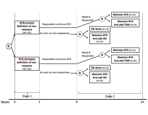
Figure 1: ExTENd study design. The ® notation represents instances of randomization; the $N$ values in this figure represent the subsequent number of patients assigned to each treatment option.

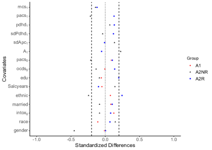
Figure 2: ExTENd study. Covariate imbalance across different treatment groups. $A_{1}$: stage 1 treatment option; $A_{2NR}$: stage 2 treatment options among non-responders; $A_{2R}$: stage 2 treatment options among responders. The dashed vertical lines show cut points at $\pm$ 0.2.

We analyzed the data using the proposed method, dWLOS${}_{m,N}^{\kappa}$ and Q-learning (Q_m,N) approaches; the results are summarized in Table 5. The latter two methods use the $N$-out-of-$N$ bootstrap for calculating standard errors in the second stage model and the $m$-out-of-$N$ bootstrap for calculating standard errors in the first stage model. Referring to earlier notation, the first stage covariate vector $\bm{W}^{0}$ consists of the predictors gender, race, alcyr${}_{0},$ intox${}_{0},$ and ocds₀, and the second stage covariate vector $\bm{S}^{0}$ consists of all the predictors listed in Table 4, along with response status. First stage regression models are fit using $\bm{W}=\bm{W}^{0}.$ The description of the second stage model predictor $\bm{S}$ is more involved. Specifically, let $\bm{Z}=(Z_{1},\ldots,Z_{6})^{\top}$ contain the variables gender, A${}_{1},$ intox₀, ocds₀, pacs₁, and mcs${}_{1};$ then, we define $\bm{S}=(\bar{R},1-\bar{R},\bar{R}Z_{1},\bar{R}Z_{2},(1-\bar{R})\bm{Z}^{\top})^{\top}$. As specified, the second stage model allows the set of possible effect modifiers to differ between responders and non-responders, with some overlap in the case of gender and A${}_{1}.$ We used SuperLearner to estimate $\mu_{1Y}(\mathbf{w}^{0})$ and $\mu_{2Y}(\mathbf{s}^{0}),$ employing the same library as we did in the simulation study and respectively using $\bm{W}^{0}$ and $\bm{S}^{0}$ for general confounding control. In view of the fact that the randomization mechanism is known, and mostly successful in view of the overall degree of balance observed in Figure 2, the treatment propensities $\mu_{1A}(\mathbf{w}^{0})$ and $\mu_{2A}(\mathbf{s}^{0})$ are estimated using logistic regression models. Specifically, the former is estimated as a function of gender, and the latter is estimated using gender, response status, and the interaction between gender and response status. The parameters of the Q-functions used by dWOLS are assumed to follow linear models (i.e., including the main effects). Similarly, for standard Q-learning, linear working models respectively replace $\eta_{2}(\bm{S}^{0})$ and $\eta_{1}(\bm{W}^{0})$.

As shown in Table 5, the signs of all predictor effects are the same for all methods, though magnitudes and confidence intervals differ. None of the effect modifiers in the second stage are deemed statistically significant among responders using any of the 3 methods. The proposed Q-learning method suggests that both ocds₀ and mcs₁ are significant effect modifiers of $A_{2}$ among non-responders; specifically, individuals with higher ocsd₀ and mcs₁ would benefit from CBI. Similarly, dWOLS identifies mcs₁ as a significant effect modifier among non-responders, whereas none of the effect modifiers are identified as significant using standard Q-learning. For the first stage model, the proposed Q-learning method shows that the years of drinking (i.e., alcyr₀) and gender significantly modify the effect of $A_{1}$. In particular, female individuals and those with more years of drinking would benefit from being treated under a stringent definition of non-response. This makes sense because, for example, individuals with more years of drinking at baseline likely have a higher craving for alcohol and require more immediate attention and rescue treatments (i.e., $A_{2}$ for non-responders). In contrast, neither standard Q-learning nor dWLOS detects any effect modifiers. With the exception of the interaction between $A_{1}$ and gender, the first stage point estimates are rather similar across the 3 methods, highlighting the fact that the differences in significance stem from the tighter confidence intervals obtained using the proposed methods (i.e., compared to those produced using the $m$-out-of-$N$ bootstrap).

Indeed, for both stages, the dWLOS and standard Q-learning methods yield point estimates that are mostly similar to each other. These similarities are expected for two reasons. First, under successful randomization, we would not generally expect misspecification of the functional form of the main effects in the Q-function to bias the estimate of interaction terms (i.e., $\bm{\beta}^{*}_{2}$). Second, the linear models being used in the Q-models are identical in both cases; the only difference is that parameter estimation is carried out using weighted versus unweighted least squares. Figure 2 demonstrates the presence of random confounding among non-responders in the second stage for gender, ethnicity, $A_{1},$ pacs₀ and pacs${}_{1},$ whereas there is good balance among the first stage predictors. Comparing dWLOS and standard Q-learning, we see that the largest differences in point estimates occur in the second stage model among non-responders for $A_{1}$ and pacs${}_{1}.$

Comparing the proposed method to both dWOLS and standard Q-learning, we observe somewhat greater disparity in point estimates. These differences occur primarily among non-responders in the second stage, and include interactions between $A_{2}$ and each of gender, $A_{1}$ and pacs${}_{1};$ as noted above, gender, $A_{1}$ and pacs₁ all demonstrate substantial imbalance among non-responders in the second stage. The largest difference among regression coefficients in the first stage model occurs for gender, consistent with the disparities observed in the second stage model as well as propagation of those differences through the backward induction process. We conjecture that modeling the true main effects (i.e., $\mu_{jY}(\cdot)$, $j=1,2$) using Super Learner may help to reduce small sample biases when compared to the more restrictive linear models used by both dWOLS and standard Q-learning.

Table 5: ExTENd data. The ^† indicates significant coefficients at a Type I error rate of 5%. CI represents the confidence interval.

Q-function	Proposed		dWLOS${}_{m,N}^{\kappa=0.05}$		Q${}_{m,N}^{\kappa=0.05}$
Models	Est	95% CI	Est	95% CI	Est	95% CI
Stage 2
Responders
$A_{2}$	0.02	(-0.07,0.11)	0.01	(-0.07,0.09)	0.01	(-0.07,0.09)
$A_{2}:gender$	0.07	(-0.11,0.24)	0.11	(-0.08,0.29)	0.11	(-0.08,0.28)
$A_{2}:A_{1}$	0.01	(-0.11,0.13)	0.01	(-0.11,0.12)	0.01	(-0.11,0.12)
Non-responders
$A_{2}$	-0.07	(-0.23,0.10)	-0.02	(-0.28,0.22)	-0.02	(-0.28,0.23)
$A_{2}:gender$	0.27	(-0.18,0.71)	0.13	(-0.43,0.81)	0.14	(-0.43,0.79)
$A_{2}:intox_{0}$	0.09	(-0.16,0.35)	0.06	(-0.21,0.46)	0.06	(-0.22,0.49)
$A_{2}:ocds_{0}$	-0.19†	(-0.34,-0.03)	-0.19	(-0.43,0.08)	-0.18	(-0.43,0.11)
$A_{2}:A_{1}$	-0.21	(-0.45,0.01)	-0.23	(-0.57,0.26)	-0.16	(-0.55,0.30)
$A_{2}:pacs_{1}$	0.10	(-0.02,0.21)	0.07	(-0.12,0.25)	0.03	(-0.18,0.23)
$A_{2}:mcs_{1}$	-0.18 †	(-0.29,-0.06)	-0.17 †	(-0.37,0.00)	-0.17	(-0.39,0.01)
Stage 1
$A_{1}$	-0.06	(-0.18,0.06)	-0.05	(-0.21,0.08)	-0.06	(-0.20,0.09)
$A_{1}:gender$	-0.24†	(-0.46,-0.01)	-0.18	(-0.43,0.14)	-0.17	(-0.37,0.14)
$A_{1}:race$	0.08	(-0.05,0.21)	0.08	(-0.07,0.21)	0.08	(-0.08,0.24)
$A_{1}:alcyr_{0}$	-0.07†	(-0.14,0.00)	-0.06	(-0.15,0.03)	-0.06	(-0.16,0.03)
$A_{1}:intox_{0}$	0.13	(-0.03,0.29)	0.14	(-0.06,0.33)	0.15	(-0.10,0.33)
$A_{1}:ocds_{0}$	0.02	(-0.05,0.09)	0.01	(-0.07,0.09)	0.01	(-0.08,0.08)

7 Discussion

Much of the current work on Q-learning continues to involve parametric working models despite the fact that finite-dimensional models are generally too restrictive to permit consistent estimation of nuisance parameters. We proposed a robust Q-learning approach where the working models need not all be linear and, specifically, where the main effects that do not influence the optimal decision rules are estimated using data-adaptive approaches. Our simulation studies highlight the value of our proposed approach compared with existing Q-learning methods. The proposed method also performed relatively well in simulations when key regularity assumption (i.e., Assumption 12) is violated; however, we cannot expect this in all scenarios, as the underlying theory and simulation results show otherwise.

An important advantage of the proposed method is that it does not suffer from the curse of dimensionality, as it produces root-$n$ consistent estimators even when $\hat{\mu}_{jA}(\cdot)$ and $\hat{\mu}_{jY}(\cdot)$ $(j=1,2)$ are estimated at rates slower than root-$n$. This important property facilitates the use of nonparametric methods like Super Learner for estimating these unknown functions, substantially reducing the chance of model misspecification. A second important feature of the proposed approach is that consistent estimation of the treatment models leads to consistent estimation of the blip function parameters, whether or not these models or those for $\mu_{jY}(\cdot),j=1,2$ are correctly specified. However, the proposed estimators are not doubly robust, in that we require that the $\mu_{jA}(\cdot)$s are consistently estimated at a sufficiently fast rate. True double robustness under (1) for $\bm{\beta}^{*}_{2}$ requires that one either consistently estimates $\mu_{2A}(\bm{S}^{0})$ or the treatment-free conditional mean model $E[Y-A_{2}\bm{S}^{\top}\bm{\beta}^{*}_{2}|\bm{S}^{0}]=\eta_{2}(\bm{S}^{0});$ similarly, for $\bm{\beta}^{*}_{1},$ one must either consistently estimate $\mu_{1A}(\bm{W}^{0})$ or $E[\tilde{Y}-A_{1}\bm{W}^{\top}\bm{\beta}^{*}_{1}|\bm{W}^{0}]=\eta_{1}(\bm{W}^{0}).$ Because the expectation operator is linear, correct specification of both treatment-free models essentially relies on both $\mu_{jY}(\cdot)$ and $\mu_{jA}(\cdot),j=1,2$ being correctly specified. This limitation on the practicality of finding a truly doubly robust estimator applies to the proposed approach as well as that taken in Wallace & Moodie (2015). Further research on doubly robust estimation in this class of problems is merited.

Although data-adaptive estimation methods reduce the risk of inconsistency, there is still a chance that one or more nuisance parameters will be estimated inconsistently. Further research is needed to study the behavior of the proposed methods under inconsistent estimation of a nuisance parameter. In particular, Benkeser et al. (2017) showed that when nuisance parameters are estimated using data-adaptive approaches, inconsistently estimating one nuisance parameter may lead to an irregular estimator having a convergence rate slower than root-$n$. These authors proposed a targeted minimum loss-based approach to resolve the issue (van der Laan, 2014). Generalization of the method of Benkeser et al. (2017) to a multi-stage decision making process would be an interesting topic for future research. Studying the asymptotic behavior of an appropriate version of the bootstrap in our proposed Q-learning method is also of interest as it can potentially resolve the non-regularity issues in settings where both Assumption 12 fails and Corollary 1 fail (e.g. Chakraborty et al., 2013). Finally, in practice, there are often many candidate variables to be considered when constructing a decision rule. The inclusion of spurious variables in these analyses can substantially reduce the quality of the estimated decision rules. Although one can adapt the proposed methods to obtain regularized estimators of the target parameters, valid post-selection inference remains a challenge and merits further research (Berk et al., 2013; Fithian et al., 2014).

Supplementary material to Robust Q-learning

Let $Z\sim P$ for some probability measure $P$ and suppose $f(\cdot)$ is any real-valued, $P-$measurable function; then, we define the $L^{2}(P)$ norm of $f(\cdot)$ as $\|f(Z)\|_{P,2}=\{\int\!f(\omega)^{2}dP(\omega)\}^{1/2}.$ In addition, let $\|\bm{x}\|_{q}$ denote the usual $q-$ norm of a vector $\bm{x}$ for $q=1,2,\infty$. The following general lemmas will be helpful in our proofs.

Lemma 1.

Let $A_{n}$ and $B_{n}$ be sequences of random vectors, $n\geq 1$. Let $\epsilon>0$ be arbitrary and, for any vector norm, suppose that $\lim_{n\rightarrow\infty}P(\|A_{n}\|>\epsilon|B_{n})=0.$ Then, $\lim_{n\rightarrow\infty}P(\|A_{n}\|>\epsilon)=0.$ By Chebyshev’s inequality, a sufficient condition for proving that $\lim_{n\rightarrow\infty}P(\|A_{n}\|>\epsilon)=0$ is that $\lim_{n\rightarrow\infty}E(\|A_{n}\|^{q}|B_{n})=0$ from some $q\geq 1.$

The above lemma essentially repeats Lemma 6.1 in Chernozhukov et al. (2018) and will not be proved here. The following lemma is a direct consequence of a well-known result and also has an easy proof; see, for example, Stewart69.

Lemma 2.

Let $\bm{M}_{n}$ and $\hat{\bm{M}}_{n}$ be two sequences of square matrices and let $\|\cdot\|$ be any proper matrix norm. Suppose there exists $n_{0}<\infty$ such that (i) $\bm{M}^{-1}_{n}$ and $\bm{M}_{n}$ exist for $n\geq n_{0}$, with $0<C_{1}\leq\|\bm{M}^{-1}_{n}\|\leq C_{2}<\infty;$ and, (ii) $\|\hat{\bm{M}}_{n}-\bm{M}_{n}\|\leq(2\|\bm{M}^{-1}_{n}\|)^{-1}$. Then,

$$\|\hat{\bm{M}}^{-1}_{n}-\bm{M}^{-1}_{n}\|\leq 2C^{2}_{2}\|\hat{\bm{M}}_{n}-\bm{M}_{n}\|.$$

We will also have need of the following lemma.

Lemma 3.

Let $\bm{B}_{1},\ldots,\bm{B}_{N}$ be independent, identically distributed vectors from $P_{0},$ where $\bm{B}_{i}\in{\mathcal{B}}\subset\mathbbmss{R}^{d}$. Let $\bm{I}_{n}$ be a randomly chosen subset of the integers $1,\ldots,N$ of length $n=O(N)$ and let its complement $\bm{I}^{c}_{n}$ have $N-n=O(N)$ elements. Let $\bm{F}_{I_{n}}$ and $\bm{F}_{I^{c}_{n}}$ be the corresponding disjoint subsets of $\bm{B}_{1},\ldots,\bm{B}_{N}.$ Let $\gamma_{j}:{\mathcal{B}}\rightarrow\mathbbmss{R},j=1,2$ and let $\hat{\gamma}_{j}(\cdot;\bm{F}_{I^{c}_{n}})$ be an estimator of $\gamma_{j}(\cdot)$ derived from the data $\bm{F}_{I^{c}_{n}}.$ Finally, define

$$\bm{G}_{n,N}=\frac{1}{n}\sum_{i\in\bm{I}_{n}}\left\{\hat{\gamma}_{1}(\bm{B}_{i};\bm{F}_{I^{c}_{n}})-\gamma_{1}(\bm{B}_{i})\right\}\left\{\hat{\gamma}_{2}(\bm{B}_{i};\bm{F}_{I^{c}_{n}})-\gamma_{2}(\bm{B}_{i})\right\}\bm{h}(\bm{B}_{i})$$ (20)

where $\bm{h}(\bm{B}_{i})$ is any finite dimensional vector- or matrix-valued function of $\bm{B}_{i}$ such that $P(\|\bm{h}(\bm{B}_{i})\|_{\infty}\leq C)=1$ for some $C<\infty$. Then,

$$\|\bm{G}_{n,N}\|_{\infty}\leq C\left\|\hat{\gamma}_{1}(\bm{B};\bm{F}_{I^{c}_{n}})-\gamma_{1}(\bm{B})\right\|_{\mathbb{P}_{n},2}\left\|\hat{\gamma}_{2}(\bm{B};\bm{F}_{I^{c}_{n}})-\gamma_{2}(\bm{B})\right\|_{\mathbb{P}_{n},2},$$ (21)

where $\mathbb{P}_{n}$ is the empirical measure on $\bm{F}_{I_{n}}$. Moreover, for $j=1,2$ define

$$\left\|\hat{\gamma}_{j}(\bm{B};\bm{F}_{I^{c}_{n}})-\gamma_{j}(\bm{B})\right\|^{2}_{P_{0},2}=\mathbbmss{E}\left\{\left\|\hat{\gamma}_{j}(\bm{B};\bm{F}_{I^{c}_{n}})-\gamma_{j}(\bm{B})\right\|^{2}_{\mathbb{P}_{n},2}\big{|}\bm{F}_{I^{c}_{n}}\right\}$$ (22)

and suppose (22) is $o_{p}(N^{-a_{j}}),$ where $a_{j}\geq 0.$ Then, $\|\bm{G}_{n,N}\|_{\infty}=o_{p}(N^{-(a_{1}+a_{2})/2})$.

Proof.

Let $r_{ij}(\bm{F}_{I^{c}_{n}})=\hat{\gamma}_{j}(\bm{B}_{i};\bm{F}_{I^{c}_{n}})-\gamma_{j}(\bm{B}_{i})$ for $i=1,\ldots,n$ and $j=1,2$. Under the assumption that $P(\|\bm{h}(\bm{B}_{i})\|_{\infty}\leq C)=1,$ the triangle and Cauchy-Schwarz equalities imply

$$\|\bm{G}_{n,N}\|_{\infty} \leq \frac{1}{n}\sum_{i\in\bm{I}_{n}}\left|r_{i1}(\bm{F}_{I^{c}_{n}})r_{i2}(\bm{F}_{I^{c}_{n}})\right|\|\bm{h}(\bm{B}_{i})\|_{\infty}$$

$$\leq C\left[\frac{1}{n}\sum_{i\in\bm{I}_{n}}\left\{r_{i1}(\bm{F}_{I^{c}_{n}})\right\}^{2}\right]^{1/2}\left[\frac{1}{n}\sum_{i\in\bm{I}_{n}}\left\{r_{i2}(\bm{F}_{I^{c}_{n}})\right\}^{2}\right]^{1/2},$$

the representation (21) now following immediately from the definition of the $L^{2}(Q)$ norm given earlier using $Q=\mathbb{P}_{n}$. To establish that $\|\bm{G}_{n,N}\|_{\infty}=o_{p}(N^{-(a_{1}+a_{2})}),$ we first use Markov’s inequality: for any $\epsilon>0,$

$$P\left(\|\bm{G}_{n,N}\|_{\infty}>\epsilon|\bm{F}_{I^{c}_{n}}\right)\leq\epsilon^{-1}\mathbbmss{E}\left(\|\bm{G}_{n,N}\|_{\infty}|\bm{F}_{I^{c}_{n}}\right).$$

Using (21) and the Cauchy-Schwarz inequality again, it follows that

$$P\left(\|\bm{G}_{n,N}\|_{\infty}>\epsilon|\bm{F}_{I^{c}_{n}}\right) \leq \frac{C}{\epsilon}\mathbbmss{E}\left\{\prod_{j=1}^{2}\left\|\hat{\gamma}_{j}(\bm{B};\bm{F}_{I^{c}_{n}})-\gamma_{j}(\bm{B})\right\|_{\mathbb{P}_{n},2}\big{|}\bm{F}_{I^{c}_{n}}\right\}$$

$$\leq \frac{C}{\epsilon}\prod_{j=1}^{2}\mathbbmss{E}\left\{\left\|\hat{\gamma}_{j}(\bm{B};\bm{F}_{I^{c}_{n}})-\gamma_{j}(\bm{B})\right\|^{2}_{\mathbb{P}_{n},2}\big{|}\bm{F}_{I^{c}_{n}}\right\}^{1/2}$$

$$= \frac{C}{\epsilon}\prod_{j=1}^{2}\left\|\hat{\gamma}_{j}(\bm{B};\bm{F}_{I^{c}_{n}})-\gamma_{j}(\bm{B})\right\|_{P_{0},2}$$

the last result following directly from (22). Under the stated assumptions, the right-hand side is now seen to be $o_{p}(N^{-(a_{1}+a_{2})/2}),$ as desired. ∎

The statement and proof of Lemma 3 employs a simple form of sample splitting in which the unknown function $\gamma_{j}(\cdot)$ is estimated by $\hat{\gamma}_{j}(\cdot;\bm{F}_{I^{c}_{n}})$ from a sample $\bm{F}_{I^{c}_{n}}$ that is independent of the $\bm{B}_{i}$s (i.e., $\bm{F}_{I_{n}}$) appearing in the calculation of (20). Importantly, Lemma 3 does not preclude the possibility that $\gamma_{1}(\cdot)=\gamma_{2}(\cdot)$ and $\hat{\gamma}_{1}(\cdot)=\hat{\gamma}_{2}(\cdot);$ in this case, (20) reduces to

$$\bm{L}_{n,m}=\frac{1}{n}\sum_{i\in\bm{I}_{n}}\left\{\hat{\gamma}(\bm{B}_{i};\bm{F}_{I^{c}_{n}})-\gamma(\bm{B}_{i})\right\}^{2}\bm{h}(\bm{B}_{i})$$ (23)

and $\|\bm{G}_{n,N}\|_{\infty}=o_{p}(N^{-a})$ for some $a\geq 0$ provided that

$$\left\|\hat{\gamma}(\bm{B};\bm{F}_{I^{c}_{n}})-\gamma(\bm{B})\right\|^{2}_{P_{0},2}=o_{p}(N^{-a}).$$ (24)

A related lemma now follows.

Lemma 4.

Let $(R_{1},\bm{B}_{1}),\ldots,(R_{n},\bm{B}_{N})$ be independent, identically distributed vectors from $P_{0},$ where $\bm{B}_{i}\in{\mathcal{B}}\subset\mathbbmss{R}^{d}$ and $E_{i}\in\mathbbmss{R}$. Suppose $\mathbbmss{E}(R_{i}|\bm{B}_{i})=0$ and $\mbox{var}(R_{i}|\bm{B}_{i})=\theta^{2}_{i}\in(0,C_{1}]$ for $i=1\ldots N$ and a constant $C_{1}<\infty.$ Let $\bm{I}_{n}$ be a randomly chosen subset of the integers $1,\ldots,N$ of length $n=O(N)$ and let its complement $\bm{I}^{c}_{n}$ have $N-n$ elements. Let $\bm{F}_{I_{n}}$ and $\bm{F}_{I^{c}_{n}}$ be the corresponding disjoint subsets of $(R_{1},\bm{B}_{1}),\ldots,(R_{N},\bm{B}_{N}).$ Let $\gamma:{\mathcal{B}}\rightarrow\mathbbmss{R}$ and let $\hat{\gamma}(\cdot;\bm{F}_{I^{c}_{n}})$ be an estimator of $\gamma(\cdot)$ derived from the data $\bm{F}_{I^{c}_{n}}.$ Finally, define

$$\bm{L}_{n,N}=\frac{1}{n}\sum_{i\in\bm{I}_{n}}R_{i}\left\{\hat{\gamma}(\bm{B}_{i};\bm{F}_{I^{c}_{n}})-\gamma(\bm{B}_{i})\right\}\bm{h}(\bm{B}_{i})$$ (25)

where $\bm{h}(\bm{B}_{i})$ is any finite dimensional vector-valued function of $\bm{B}_{i}$ such that $P(\|\bm{h}(\bm{B}_{i})\|_{2}\leq C_{2})=1$ for $C_{2}<\infty$. Suppose that

$$\left\|\hat{\gamma}(\bm{B};\bm{F}_{I^{c}_{n}})-\gamma(\bm{B})\right\|^{2}_{P_{0},2}=\mathbbmss{E}\left\{\left\|\hat{\gamma}(\bm{B};\bm{F}_{I^{c}_{n}})-\gamma(\bm{B})\right\|^{2}_{\mathbb{P}_{n},2}\big{|}\bm{F}_{I^{c}_{n}}\right\}$$ (26)

is $o_{p}(N^{-a})$ where $a\geq 0.$ Then, $\|\bm{L}_{n,N}\|_{\infty}=o_{p}(N^{-(1+a)/2}).$

Proof.

The proof relies on a variant of Chebyshev’s inequality. Let

$$\bm{L}_{n,N,j}=\frac{1}{n}\sum_{i\in\bm{I}_{n}}R_{i}\left\{\hat{\gamma}(\bm{B}_{i};\bm{F}_{I^{c}_{n}})-\gamma(\bm{B}_{i})\right\}\bm{h}_{j}(\bm{B}_{i})$$

be the $j^{th}$ element of $\bm{L}_{n,N}.$ Let ${\mathcal{B}}_{n}=\{\bm{I}_{n},(\bm{B}_{k},k\in\bm{I}_{n})\}.$ Then, it is easy to show that

$$\mathbbmss{E}\left(\bm{L}_{n,N,j}\big{|}\bm{F}_{I^{c}_{n}}\right)~{}=~{}\mathbbmss{E}\left\{\mathbbmss{E}\left(\bm{L}_{n,N,j}\big{|}\bm{F}_{I^{c}_{n}},{\mathcal{B}}_{n}\right)\big{|}\bm{F}_{I^{c}_{n}}\right\}~{}=~{}0;$$

this follows from calculating the inner expectation on the right-hand-side and using the assumption that $\mathbbmss{E}(R_{i}|\bm{B}_{i})=0$ for every $i.$ Using a similar conditioning argument,

$$\mbox{var}\left(\bm{L}_{n,N,j}\big{|}\bm{F}_{I^{c}_{n}}\right) = \mathbbmss{E}\left\{\mbox{var}\left(\bm{L}_{n,N,j}\big{|}\bm{F}_{I^{c}_{n}},{\mathcal{B}}_{n}\right)\big{|}\bm{F}_{I^{c}_{n}}\right\}.$$

Straightforward calculations now show

$$\mbox{var}\left(\bm{L}_{n,N,j}\big{|}\bm{F}_{I^{c}_{n}},{\mathcal{B}}_{n}\right) = \frac{1}{n^{2}}\sum_{i\in\bm{I}_{n}}\left\{\hat{\gamma}(\bm{B}_{i};\bm{F}_{I^{c}_{n}})-\gamma(\bm{B}_{i})\right\}^{2}\bm{h}^{2}_{j}(\bm{B}_{i})\mbox{var}\left(R_{i}|\bm{B}_{i}\right),$$

implying that

$$\mbox{var}\left(\bm{L}_{n,N,j}\big{|}\bm{F}_{I^{c}_{n}}\right) = \mathbbmss{E}\left[\frac{1}{n^{2}}\sum_{i\in\bm{I}_{n}}\left\{\hat{\gamma}(\bm{B}_{i};\bm{F}_{I^{c}_{n}})-\gamma(\bm{B}_{i})\right\}^{2}\bm{h}^{2}_{j}(\bm{B}_{i})\theta^{2}_{i}\Big{|}\bm{F}_{I^{c}_{n}}\right]$$

$$\leq \frac{C_{1}C_{2}}{n}\mathbbmss{E}\left[\frac{1}{n}\sum_{i\in\bm{I}_{n}}\left\{\hat{\gamma}(\bm{B}_{i};\bm{F}_{I^{c}_{n}})-\gamma(\bm{B}_{i})\right\}^{2}\Big{|}\bm{F}_{I^{c}_{n}}\right]$$

$$= \frac{C_{1}C_{2}}{n}\left\|\hat{\gamma}(\bm{B};\bm{F}_{I^{c}_{n}})-\gamma(\bm{B})\right\|^{2}_{P_{0},2}$$

$$= o_{p}(N^{-(1+a)}),$$

the last step following from the assumptions on (26) made in the statement of the lemma and the fact that $n=O(N)$. Using a vector form of Chebyshev’s inequality, it can then be shown that $\|\bm{L}_{n,N}\|_{2}=o_{p}(N^{-(1+a)/2});$ since $\|\bm{L}_{n,N}\|_{\infty}\leq\|\bm{L}_{n,N}\|_{2}$, the stated result follows. ∎

8 Proof of Theorem 1

To review our main assumptions, we assume that we observe $N$ independently identically distributed trajectories of $(\bm{X}_{1},A_{1},\bm{X}_{2},A_{2},Y)\sim P_{0}$. The vector $\bm{X}_{1}\in\mathcal{X}_{1}\subset\mathbbmss{R}^{p_{1}}$ consists of baseline covariates measured before treatment at the first decision point $A_{1}\in\{0,1\}$ and the vector $\bm{X}_{2}\in\mathcal{X}_{2}\subset\mathbbmss{R}^{p_{2}}$ consists of intermediate covariates measured before treatment at the second decision point $A_{2}\in\{0,1\}$. For notational convenience we define $\bm{S}^{0}_{i}=(\bm{X}_{1i}^{\top},A_{1i},\bm{X}_{2i}^{\top})^{\top}\in\mathcal{S}\subset\mathbbmss{R}^{p_{1}+p_{2}+1}$ and $\bm{W}^{0}_{i}=\bm{X}_{1i}\in\mathcal{X}_{1}\subset\mathbbmss{R}^{p_{1}}$. We will also have need to define the variables $\bm{S}_{i}$ and $\bm{W}_{i},i=1,\ldots,N;$ respectively, each represents some finite dimensional function of the variables in $\bm{S}^{0}_{i}$ and $\bm{W}^{0}_{i}.$ We note that knowledge of $\bm{S}^{0}_{i}$ and $\bm{W}^{0}_{i}$ respectively implies knowledge of $\bm{S}_{i}$ and $\bm{W}_{i};$ however, the reverse may not hold. The observed outcome $Y\in\mathbbmss{R}$ (measured after $A_{2}$) is assumed continuous, with a larger value of $Y$ indicating a better clinical outcome.

The developments below assume that the original sample, with elements independently and identically distributed as $P_{0},$ has been split into two independent samples, say $\bm{D}_{I_{n}}$ and $\bm{D}_{I^{c}_{n}},$ being respectively of sizes $n=O(N)$ and $N-n=O(N)$. The nuisance parameters $\hat{\mu}_{2Y}(\cdot),$ $\hat{\mu}_{2A}(\cdot),$ $\hat{\mu}_{1Y}(\cdot),$ and $\hat{\mu}_{1A}(\cdot)$ are estimated using the data in $\bm{D}_{I^{c}_{n}};$ the finite dimensional parameters of interest are then estimated using the data $\bm{D}_{I_{n}},$ treating $\hat{\mu}_{2Y}(\cdot),$ $\hat{\mu}_{2A}(\cdot),$ $\hat{\mu}_{1Y}(\cdot),$ and $\hat{\mu}_{1A}(\cdot)$ as if they were known functions. As developed here, our use of sample-splitting is a simple form of cross-fitting and can be generalized easily to make better use of the full sample (Chernozhukov et al., 2018); the simpler form used here suffices to establish the main ideas of the proofs. Lemmas 3 and 4 play an important role in several of the proofs; since $n=O(N),$ statements of the form $o_{p}(N^{-a})$ and $o_{p}(n^{-1})$ are equivalent, we use the latter to emphasize that the technical arguments rely on sample splitting, where a sample $\bm{D}_{I_{n}}$ of size $n$ is used to estimate the finite dimensional parameters of interest.

To simplify notation, where needed all calculations implicitly condition on the set of selected indices $\bm{I}_{n}$. Using notation from the main paper, let $\Delta_{2i}=\Delta_{2}(\bm{S}^{0}_{i}),$ $\Delta_{1i}=\Delta_{1}(\bm{W}^{0}_{i}),$ $\mu_{2Ai}=\mu_{2A}(\bm{S}^{0}_{i}),$ $\hat{\mu}_{2Ai}=\hat{\mu}_{2A}(\bm{S}^{0}_{i}),$ $\mu_{1Ai}=\mu_{1A}(\bm{W}^{0}_{i}),$ and $\hat{\mu}_{1Ai}=\hat{\mu}_{1A}(\bm{W}^{0}_{i}).$ In addition, as in the main paper, we define the matrices

$$\mathbf{V}_{2n}=\frac{1}{n}\sum_{i\in\bm{I}_{n}}(A_{2i}-\mu_{2Ai})^{2}\bm{S}^{\otimes 2}_{i}~{}\mbox{ and }~{}\hat{\mathbf{V}}_{2n}=\frac{1}{n}\sum_{i\in\bm{I}_{n}}(A_{2i}-\hat{\mu}_{2Ai})^{2}\bm{S}^{\otimes 2}_{i}$$

$$\mathbf{V}_{1n}=\frac{1}{n}\sum_{i\in\bm{I}_{n}}(A_{1i}-\hat{\mu}_{1Ai})^{2}\bm{W}^{\otimes 2}_{i}~{}\mbox{ and }~{}\hat{\mathbf{V}}_{1n}=\frac{1}{n}\sum_{i\in\bm{I}_{n}}(A_{1i}-\hat{\mu}_{1Ai})^{2}\bm{W}^{\otimes 2}_{i}$$

where $\bm{x}^{\otimes 2}=\bm{x}\bm{x}^{\top}$ for any vector $\bm{x}$.

We make the following assumptions.

Assumption 7.

(i) The support of $\bm{W}^{0}$ and the conditional treatment effect $\Delta_{1}(\bm{W}^{0})$ are uniformly bounded; (ii) the support of $\bm{S}^{0}$ and the conditional treatment effect $\Delta_{2}(\bm{S}^{0})$ are uniformly bounded; and, the supports of $\bm{S}$ and $\bm{W}$ are uniformly bounded.

Assumption 8.

(i) $\left\|\hat{\mu}_{1A}(\bm{W}^{0};\bm{D}_{I^{c}_{n}})-\mu_{1A}(\bm{W}^{0})\right\|^{2}_{P_{0},2}=o_{p}(n^{-1/2});$ (ii) $\left\|\hat{\mu}_{2A}(\bm{S}^{0};\bm{D}_{I^{c}_{n}})-\mu_{2A}(\bm{S}^{0})\right\|^{2}_{P_{0},2}=o_{p}(n^{-1/2}).$

Assumption 9.

(i) $\left\|\hat{\mu}_{1Y}(\bm{W}^{0};\bm{D}_{I^{c}_{n}})-\mu_{1Y}(\bm{W}^{0})\right\|^{2}_{P_{0},2}=o_{p}(1);$ (ii) $\left\|\hat{\mu}_{2Y}(\bm{S}^{0};\bm{D}_{I^{c}_{n}})-\mu_{2Y}(\bm{S}^{0})\right\|^{2}_{P_{0},2}=o_{p}(1).$

Assumption 10.

(i) $\left\|\hat{\mu}_{1Y}(\bm{W}^{0};\bm{D}_{I^{c}_{n}})-\mu_{1Y}(\bm{W}^{0})\right\|_{P_{0},2}\left\|\hat{\mu}_{1A}(\bm{W}^{0};\bm{D}_{I^{c}_{n}})-\mu_{1A}(\bm{W}^{0})\right\|_{P_{0},2}=o_{p}(n^{-1/2});$
(ii) $\left\|\hat{\mu}_{2Y}(\bm{S}^{0};\bm{D}_{I^{c}_{n}})-\mu_{2Y}(\bm{S}^{0})\right\|_{P_{0},2}\left\|\hat{\mu}_{2A}(\bm{S}^{0};\bm{D}_{I^{c}_{n}})-\mu_{2A}(\bm{S}^{0})\right\|_{P_{0},2}=o_{p}(n^{-1/2})$

Assumption 11.

There exists $1\leq n_{0}<\infty$ such that $\mathbf{V}_{jn}$ and $\hat{\mathbf{V}}_{jn},j=1,2$ are positive definite for $n\geq n_{0}$.

Assumption 12.

$P\big{(}|\bm{S}_{1}^{\top}\bm{\beta}^{*}_{2}|=0\big{)}=0.$

We prove this Theorem with help from the following lemma.

Lemma 5.

Suppose Assumptions 7, 8, and 11 hold. Let $d_{2}=dim(\bm{S})$ and $d_{1}=dim(\bm{W})$. Then $\|\tilde{\bm{\beta}}^{*}_{2n}-{\bm{\beta}}^{*}_{2n}\|_{\infty}=o_{p}(n^{-1/2})$ and $\|\tilde{\bm{\beta}}^{*}_{1n}-{\bm{\beta}}^{*}_{1n}\|_{\infty}=o_{p}(n^{-1/2})$, where

$$\tilde{\bm{\beta}}^{*}_{2n} =\operatorname*{argmin}_{\bm{\beta}_{2}\in\mathbbmss{R}^{d_{2}}}\sum_{i\in\bm{I}_{n}}\left\{A_{2i}-\hat{\mu}_{2A}(\bm{S}^{0}_{i})\right\}^{2}\left\{\Delta_{2}(\bm{S}^{0}_{i})-\bm{S}^{\top}_{i}\bm{\beta}_{2}\right\}^{2},$$

$$\bm{\beta}^{*}_{2n} =\operatorname*{argmin}_{\bm{\beta}_{2}\in\mathbbmss{R}^{d_{2}}}\sum_{i\in\bm{I}_{n}}\left\{A_{2i}-\mu_{2A}(\bm{S}^{0}_{i})\right\}^{2}\left\{\Delta_{2}(\bm{S}^{0}_{i})-\bm{S}^{\top}_{i}\bm{\beta}_{2}\right\}^{2},$$

$$\tilde{\bm{\beta}}^{*}_{1n} =\operatorname*{argmin}_{\bm{\beta}_{1}\in\mathbbmss{R}^{d_{1}}}\sum_{i\in\bm{I}_{n}}\left\{A_{1i}-\hat{\mu}_{1A}(\bm{W}_{i})\right\}^{2}\left\{\Delta_{1}(\bm{W}^{0}_{i})-\bm{W}^{\top}_{i}\bm{\beta}_{1}\right\}^{2},$$

$$\bm{\beta}^{*}_{1n} =\operatorname*{argmin}_{\bm{\beta}_{1}\in\mathbbmss{R}^{d_{1}}}\sum_{i\in\bm{I}_{n}}\left\{A_{1i}-\mu_{1A}(\bm{W}_{i})\right\}^{2}\left\{\Delta_{1}(\bm{W}^{0}_{i})-\bm{W}^{\top}_{i}\bm{\beta}_{1}\right\}^{2}.$$

Proof.

Below, we will prove that $\|\tilde{\bm{\beta}}^{*}_{2n}-{\bm{\beta}}^{*}_{2n}\|_{\infty}=o_{p}(n^{-1/2});$ the result that $\|\tilde{\bm{\beta}}^{*}_{1n}-{\bm{\beta}}^{*}_{1n}\|_{\infty}=o_{p}(n^{-1/2})$ follows from essentially identical arguments. Using the definitions of $\tilde{\bm{\beta}}^{*}_{2n}$ and ${\bm{\beta}}^{*}_{2n}$ and assuming $n$ is large enough so that Assumption 11 holds, straightforward algebra shows

$$\tilde{\bm{\beta}}^{*}_{2n}-{\bm{\beta}}^{*}_{2n}= (\hat{\mathbf{V}}_{2n}^{-1}-\mathbf{V}_{2n}^{-1})\left\{\frac{1}{n}\sum_{i\in\bm{I}_{n}}(A_{2i}-\mu_{2Ai})^{2}\bm{S}_{i}\Delta_{2i}\right\}$$

$$+\hat{\mathbf{V}}_{2n}^{-1}\left\{\frac{1}{n}\sum_{i\in\bm{I}_{n}}(\mu_{2Ai}-\hat{\mu}_{2Ai})^{2}\bm{S}_{i}\Delta_{2i}\right\}.$$

Taking norms and using the triangle inequality, it can be shown that

$$\sqrt{n}\|\tilde{\bm{\beta}}^{*}_{2n}-{\bm{\beta}}^{*}_{2n}\|_{\infty}\leq\sqrt{n}\bigl{\|}\hat{\mathbf{V}}_{2n}^{-1}-\mathbf{V}_{2n}^{-1}\bigr{\|}_{\infty}\,(A_{n}+B_{n})+\sqrt{n}\bigl{\|}\mathbf{V}_{2n}^{-1}\bigr{\|}_{\infty}\,B_{n}$$ (27)

where

$$A_{n} =\bigg{\|}\frac{1}{n}\sum_{i\in\bm{I}_{n}}(A_{2i}-\mu_{2Ai})^{2}\bm{S}_{i}\Delta_{2i}\biggr{\|}_{\infty}$$

$$B_{n} =\bigg{\|}\frac{1}{n}\sum_{i\in\bm{I}_{n}}(\hat{\mu}_{2Ai}-\mu_{2Ai})^{2}\bm{S}_{i}\Delta_{2i}\biggr{\|}_{\infty}.$$

Suppose that $\|\hat{\mathbf{V}}_{2n}-\mathbf{V}_{2n}\|_{\infty}=o_{p}(n^{-1/2}).$ Then, by Lemma 2 and Assumption 11, we have for $n$ sufficiently large that

$$\|\hat{\mathbf{V}}_{2n}^{-1}-\mathbf{V}_{2n}^{-1}\|_{\infty}\leq K_{1}\|\hat{\mathbf{V}}_{2n}-\mathbf{V}_{2n}\|_{\infty}$$ (28)

for any constant $K_{1}$ such that $2\|\mathbf{V}_{2n}^{-1}\|^{2}_{\infty}\leq K_{1}$. It can be seen that

$$A_{n}\stackrel{{\scriptstyle p}}{{\rightarrow}}\Big{\|}\mathbbmss{E}\left[\{A_{2}-\mu_{2A}(\bm{S}^{0})\}^{2}\bm{S}\Delta_{2}(\bm{S}^{0})\right]\Bigr{\|}_{\infty}=\Big{\|}\mathbbmss{E}\left[\bm{S}\Delta_{2}(\bm{S}^{0})\mbox{var}(A_{2}|\bm{S}^{0})\right]\Bigr{\|}_{\infty}<\infty.$$

Since cross-fitting is used to estimate $\hat{\mu}_{2A}(\cdot),$ we also see that $B_{n}$ is an example of (23); hence, using Lemma 3 and Assumption 8, it follows that $B_{n}=o_{p}(n^{-1/2}).$ It follows from these results and (28) that (27) is $o_{p}(1).$

In order to prove that $\|\hat{\mathbf{V}}_{2n}-\mathbf{V}_{2n}\|_{\infty}=o_{p}(n^{-1/2}),$ we begin by writing $\|\hat{\mathbf{V}}_{2n}-\mathbf{V}_{2n}\|_{\infty}\leq C_{n}+2D_{n},$ where

$$C_{n} =\left\|\frac{1}{n}\sum_{i\in\bm{I}_{n}}(\mu_{2Ai}-\hat{\mu}_{2Ai})^{2}\bm{S}^{\otimes 2}_{i}\right\|_{\infty}$$

$$D_{n} =\left\|\frac{1}{n}\sum_{i\in\bm{I}_{n}}(A_{2i}-\mu_{2Ai})(\hat{\mu}_{2Ai}-\mu_{2Ai})\bm{S}^{\otimes 2}_{i}\right\|_{\infty}.$$

Again, because cross-fitting is used to estimate $\hat{\mu}_{2A}(\cdot),$ we can see that $C_{n}$ is also an example of (23) and it follows by previously stated arguments that $C_{n}=o_{p}(n^{-1/2})$. In order to establish the behavior of $D_{n}$, we first note that $D_{n}=\max_{j=1,\ldots,d_{2}}\sum_{k=1}^{d_{2}}\left|H_{njk}\right|$ where $d_{2}$ is finite and

$$H_{njk}=\frac{1}{n}\sum_{i\in\bm{I}_{n}}(A_{2i}-\mu_{2Ai})(\hat{\mu}_{2Ai}-\mu_{2Ai})S_{ik}S_{ij}.$$

It suffices to establish the behavior of $H_{njk}$. First, using the definition of $\mu_{2Ai}=\mu_{2A}(\bm{S}^{0}_{i})=\mathbbmss{E}(A_{2i}|\bm{S}^{0}_{i})$ and the fact that $\hat{\mu}_{2Ai}=\hat{\mu}_{2A}(\bm{S}^{0}_{i})$ where $\hat{\mu}_{2A}(\cdot)$ is estimated from data $\bm{D}_{I^{c}_{n}}$ that is independent of $\bm{S}^{0}_{i}\in\bm{D}_{I_{n}}$ for each $i,$ it is easy to see that $\mathbbmss{E}(H_{njk}|\bm{S}^{0}_{1},\ldots,\bm{S}^{0}_{n},\bm{D}_{I^{c}_{n}})=0$ and hence that $\mathbbmss{E}(H_{njk}|\bm{D}_{I^{c}_{n}})=0.$ Using these same properties, it is also easily shown that

$$\mbox{var}(H_{njk}|\bm{D}_{I^{c}_{n}})=\frac{1}{n^{2}}\sum_{i\in\bm{I}_{n}}\mathbbmss{E}\left\{(\hat{\mu}_{2Ai}-\mu_{2Ai})^{2}\mbox{var}(A_{2i}|\bm{S}^{0}_{i})(S_{ik}S_{ij})^{2}|\bm{D}_{I^{c}_{n}}\right\}.$$

Under Assumption 7, we can find a constant $K_{2}<\infty$ such that

$$\mbox{var}(H_{njk}|\bm{D}_{I^{c}_{n}}) \leq \frac{K_{2}}{n}\mathbbmss{E}\left[\frac{1}{n}\sum_{i\in\bm{I}_{n}}\{\hat{\mu}_{2A}(\bm{S}^{0}_{i})-\mu_{2A}(\bm{S}^{0}_{i})\}^{2}\Big{|}\bm{D}_{I^{c}_{n}}\right]$$

$$= \frac{K_{2}}{n}\mathbbmss{E}\left\{\|\hat{\mu}_{2A}(\bm{S}^{0};\bm{D}_{I^{c}_{n}})-\mu_{2A}(\bm{S}^{0})\|^{2}_{\mathbb{P}_{n},2}\Big{|}\bm{D}_{I^{c}_{n}}\right\}$$

$$= \frac{K_{2}}{n}\|\hat{\mu}_{2A}(\bm{S}^{0};\bm{D}_{I^{c}_{n}})-\mu_{2A}(\bm{S}^{0})\|^{2}_{P_{0},2},$$

By Chebyshev’s inequality, for all $\epsilon>0$ we then have

$$P\left(n^{1/2}\left|H_{njk}\right|>\epsilon\bigl{|}\bm{D}_{I^{c}_{n}}\right)\leq\frac{K_{2}}{\epsilon^{2}}\|\hat{\mu}_{2A}(\bm{S}^{0};\bm{D}_{I^{c}_{n}})-\mu_{2A}(\bm{S}^{0})\|^{2}_{P_{0},2},$$

where the right-hand side is $o_{p}(n^{-1/2})$ by Assumption 8. Lemma 1 now implies that $H_{njk}=o_{p}(n^{-1/2})$ and hence that $D_{n}=o_{p}(n^{-1/2}).$ Therefore, $\|\hat{\mathbf{V}}_{2n}-\mathbf{V}_{2n}\|_{\infty}\leq C_{n}+2D_{n}=o_{p}(n^{-1/2}),$ proving the desired result. A similar argument shows $\sqrt{n}\|\tilde{\bm{\beta}}^{*}_{1n}-{\bm{\beta}}^{*}_{1n}\|_{\infty}=o_{p}(1)$. ∎

As in the main paper, we define

$$\bm{\beta}^{*}_{2} = \operatorname*{argmin}_{\bm{\beta}_{2}\in\mathbbmss{R}^{d_{2}}}\mathbbmss{E}\left[\mbox{var}\left(A_{2}|\bm{S}^{0}\right)\left\{\Delta_{2}(\bm{S}^{0})-\bm{S}^{\top}\bm{\beta}_{2}\right\}^{2}\right],$$ (29)

$$\mathbf{V}_{2} = \mathbbmss{E}\left\{\mbox{var}\left(A_{2}|\bm{S}^{0}\right)\bm{S}^{\otimes 2}\right\}$$ (30)

$$\bm{\beta}^{*}_{1} = \operatorname*{argmin}_{\bm{\beta}_{1}\in\mathbbmss{R}^{d_{1}}}\mathbbmss{E}\left[\mbox{var}\left(A_{1}|\bm{W}^{0}\right)\left\{\Delta_{1}(\bm{W}^{0})-\bm{W}^{\top}\bm{\beta}_{1}\right\}^{2}\right],$$ (31)

$$\mathbf{V}_{1} = \mathbbmss{E}\left\{\mbox{var}\left(A_{1}|\bm{W}^{0}\right)\bm{W}^{\otimes 2}\right\}.$$ (32)

As $n\rightarrow\infty$, it is easy to see that $\bm{\beta}^{*}_{2n}$ converges to

$$\bm{\beta}^{*}_{2}=\mathbf{V}_{2}^{-1}\mathbbmss{E}\left\{\mbox{var}\left(A_{2}|\bm{S}^{0}\right)\bm{S}\Delta_{2}(\bm{S}^{0})\right\};$$

similarly, $\bm{\beta}^{*}_{1n}$ converges to

$$\bm{\beta}^{*}_{1}=\mathbf{V}_{1}^{-1}\mathbbmss{E}\left\{\mbox{var}\left(A_{1}|\bm{W}^{0}\right)\bm{W}\Delta_{1}(\bm{W}^{0})\right\}.$$

With these preliminaries in place, we can now prove the main result.

Proof of Theorem 1, part (a).

We desire to show that $\hat{\bm{\beta}}_{2n}$ is an asymptotically linear estimator of $\bm{\beta}_{2}^{*}$ with the claimed influence function, where $\bm{\beta}^{*}_{2}$ is defined in (29) and

$$\hat{\bm{\beta}}_{2n} =\operatorname*{argmin}_{\bm{\beta}_{2}\in\mathbbmss{R}^{d_{2}}}\sum_{i\in\bm{I}_{n}}\left[Y_{i}-\hat{\mu}_{2Y}(\bm{S}^{0}_{i})-\{A_{2i}-\hat{\mu}_{2A}(\bm{S}^{0}_{i})\}\cdot\bm{S}_{i}^{\top}\bm{\beta}_{2}\right]^{2}.$$

In view of Lemma 5, we can proceed by establishing asymptotically linear representations for both $\sqrt{n}(\hat{\bm{\beta}}_{2n}-\tilde{\bm{\beta}}^{*}_{2n})$ and $\sqrt{n}({\bm{\beta}}^{*}_{2n}-{\bm{\beta}}^{*}_{2});$ combined, these will lead to that for $\sqrt{n}(\hat{\bm{\beta}}_{2n}-{\bm{\beta}}^{*}_{2}).$

Recalling notation introduced earlier, it is easy to show that

$$\sqrt{n}(\hat{\bm{\beta}}_{2n} -\tilde{\bm{\beta}}^{*}_{2n})=$$

$$\hat{\mathbf{V}}_{2n}^{-1}\left[\frac{1}{\sqrt{n}}\sum_{i\in\bm{I}_{n}}(A_{2i}-\hat{\mu}_{2Ai})\bm{S}_{i}\{Y_{i}-\hat{\mu}_{2Yi}-(A_{2i}-\hat{\mu}_{2Ai})\Delta_{2i}\}\right]$$ (33)

By adding and subtracting terms and using the model assumptions on $Y_{i}$, one can write

$$Y_{i}-\hat{\mu}_{2Yi}-(A_{2i}-\hat{\mu}_{2Ai})\Delta_{2i}=\epsilon_{2i}+(\mu_{2Yi}-\hat{\mu}_{2Yi})+(\hat{\mu}_{2Ai}-\mu_{2Ai})\Delta_{2i}.$$ (34)

The decomposition (34) implies that the term in the square brackets on the right-hand side of (33) can be decomposed into six terms:

$$\frac{1}{\sqrt{n}}\sum_{i\in\bm{I}_{n}}(A_{2i}-\hat{\mu}_{2Ai}) \bm{S}_{i}\{Y_{i}-\hat{\mu}_{2Yi}-(A_{2i}-\mu_{2Ai})\Delta_{2i}\}$$ (35)

$$=\frac{1}{\sqrt{n}}\sum_{i\in\bm{I}_{n}}\epsilon_{2i}(A_{2i}-\mu_{2Ai})\bm{S}_{i}$$ (36)

$$-\frac{1}{\sqrt{n}}\sum_{i\in\bm{I}_{n}}(A_{2i}-\mu_{2Ai})(\hat{\mu}_{2Yi}-\mu_{2Yi})\bm{S}_{i}$$ (37)

$$+\frac{1}{\sqrt{n}}\sum_{i\in\bm{I}_{n}}(A_{2i}-\mu_{2Ai})(\hat{\mu}_{2Ai}-\mu_{2Ai})\Delta_{2i}\bm{S}_{i}$$ (38)

$$-\frac{1}{\sqrt{n}}\sum_{i\in\bm{I}_{n}}\epsilon_{2i}(\hat{\mu}_{2Ai}-\mu_{2Ai})\bm{S}_{i}$$ (39)

$$+\frac{1}{\sqrt{n}}\sum_{i\in\bm{I}_{n}}(\hat{\mu}_{2Ai}-\mu_{2Ai})(\hat{\mu}_{2Yi}-\mu_{2Yi})\bm{S}_{i}$$ (40)

$$-\frac{1}{\sqrt{n}}\sum_{i\in\bm{I}_{n}}(\hat{\mu}_{2Ai}-\hat{\mu}_{2Ai})^{2}\Delta_{2i}\bm{S}_{i}.$$ (41)

Under the assumptions of this theorem, the central limit theorem establishes the asymptotic normality of (36), which is $O_{p}(1)$. The terms (37)-(39) are each seen to be examples to which Lemma 4 applies; under Assumptions 7-11, it follows that each term is $o_{p}(1)$. The terms (40) and (41) are both seen to be examples to which Lemma 3 applies; again, under Assumptions 7-11, each term is $o_{p}(1).$ Because $\|\hat{\mathbf{V}}_{2n}^{-1}-\mathbf{V}^{-1}_{2n}\|_{\infty}=o_{p}(1)$ it follows that $\sqrt{n}(\hat{\bm{\beta}}_{2n}-\tilde{\bm{\beta}}^{*}_{2n})$ can be written

$$\sqrt{n}(\hat{\bm{\beta}}_{2n}-\tilde{\bm{\beta}}^{*}_{2n})=\frac{1}{\sqrt{n}}\sum_{i\in\bm{I}_{n}}\mathbf{V}^{-1}_{2n}\epsilon_{2i}(A_{2i}-\mu_{2Ai})\bm{S}_{i}+o_{p}(1).$$ (42)

Turning to $\sqrt{n}({\bm{\beta}}^{*}_{2n}-{\bm{\beta}}^{*}_{2}),$ we can write

$$\sqrt{n}({\bm{\beta}}^{*}_{2n}-{\bm{\beta}}^{*}_{2}) =\sqrt{n}\left[\biggl{\{}n^{-1}\sum_{i\in\bm{I}_{n}}\mathbf{V}^{-1}_{2n}(A_{2i}-\mu_{2Ai})^{2}\Delta_{2i}\bm{S}_{i}\biggr{\}}-{\bm{\beta}}^{*}_{2}\right]$$

$$=\frac{1}{\sqrt{n}}\mathbf{V}^{-1}_{2n}\sum_{i\in\bm{I}_{n}}(A_{2i}-\mu_{2Ai})^{2}\bm{S}_{i}\bigl{(}\Delta_{2i}-\bm{S}^{\top}_{i}{\bm{\beta}}^{*}_{2}\bigr{)}.$$ (43)

Hence, using (42) and (43) and collecting terms,

$$\sqrt{n}(\hat{\bm{\beta}}_{2n}-{\bm{\beta}}^{*}_{2})=\frac{1}{\sqrt{n}}\mathbf{V}^{-1}_{2n}\sum_{i\in\bm{I}_{n}}(A_{2i}-\mu_{2Ai})\bm{S}_{i}H_{2i}+o_{p}(1)$$

where $H_{2i}=\epsilon_{2i}+(A_{2i}-\mu_{2Ai})\bigl{(}\Delta_{2i}-\bm{S}^{\top}_{i}{\bm{\beta}}^{*}_{2}\bigr{)}.$ Using the fact that $Y_{i}-\mu_{2Yi}=\epsilon_{2i}+(A_{2i}-\mu_{2Ai})\Delta_{2i},$ we may write

$$H_{2i} = Y_{i}-\mu_{2Yi}-(A_{2i}-\mu_{2Ai})\Delta_{2i}+(A_{2i}-\mu_{2Ai})\bigl{(}\Delta_{2i}-\bm{S}^{\top}_{i}{\bm{\beta}}^{*}_{2}\bigr{)}$$ (44)

$$= Y_{i}-\mu_{2Yi}-(A_{2i}-\mu_{2Ai})\bm{S}^{\top}_{i}{\bm{\beta}}^{*}_{2}.$$

Consequently,

$$\sqrt{n}(\hat{\bm{\beta}}_{2n}-{\bm{\beta}}^{*}_{2})=\frac{1}{\sqrt{n}}\sum_{i\in\bm{I}_{n}}\mbox{\rm Inf}_{2in}+o_{p}(1)$$

where

$$\mbox{\rm Inf}_{2in}=\mathbf{V}^{-1}_{2n}(A_{2i}-\mu_{2Ai})\bm{S}_{i}\bigl{\{}Y_{i}-\mu_{2Yi}-(A_{2i}-\mu_{2Ai})\bm{S}^{\top}_{i}{\bm{\beta}}^{*}_{2}\bigr{\}}.$$

Since $\|\mathbf{V}_{2n}^{-1}-\mathbf{V}^{-1}_{2}\|_{\infty}=o_{p}(1),$ it now follows that

$$\sqrt{n}(\hat{\bm{\beta}}_{2n}-{\bm{\beta}}^{*}_{2})=\frac{1}{\sqrt{n}}\sum_{i\in\bm{I}_{n}}\mbox{\rm Inf}_{2i}+o_{p}(1),$$

where

$$\mbox{\rm Inf}_{2i}=\mathbf{V}^{-1}_{2}(A_{2i}-\mu_{2Ai})\bm{S}_{i}\bigl{\{}Y_{i}-\mu_{2Yi}-(A_{2i}-\mu_{2Ai})\bm{S}^{\top}_{i}{\bm{\beta}}^{*}_{2}\bigr{\}}$$ (45)

has mean zero and variance $\mathbf{V}^{-1}_{2}\bm{Q}_{2}\mathbf{V}^{-1}_{2}$ where $\mathbf{Q}_{2}=\mathbbmss{E}(\bm{J}_{2}^{\otimes 2})$ and

$$\bm{J}_{2}=\{A_{2}-\mu_{2A}(\bm{S}^{0})\}\bm{S}\left[Y-\mu_{2Y}(\bm{S}^{0})-\{A_{2}-\mu_{2A}(\bm{S}^{0})\}\bm{S}^{\top}{\bm{\beta}}^{*}_{2}\right].$$ (46)

∎

Proof of Theorem 1, part (b).

As in part (a), we need to show that $\hat{\bm{\beta}}_{1n}$ is an asymptotically linear estimator of $\bm{\beta}_{1}^{*}$ with a certain influence function, where $\bm{\beta}^{*}_{1}$ is defined in (31) and

$$\hat{\bm{\beta}}_{1n} =\operatorname*{argmin}_{\bm{\beta}_{1}\in\mathbbmss{R}^{d_{1}}}\sum_{i\in\bm{I}_{n}}\left[\hat{\tilde{Y}}_{i}-\hat{\mu}_{1Y}(\bm{W}^{0}_{i})-\{A_{1i}-\hat{\mu}_{1A}(\bm{W}^{0}_{i})\}\cdot\bm{W}_{i}^{\top}\bm{\beta}_{1}\right]^{2},$$

where $\hat{\tilde{Y}}_{i}$ is calculated as

$$\hat{\tilde{Y}}_{i}=Y_{i}+\bm{S}_{i}^{\top}\hat{\bm{\beta}}_{2n}\bigl{\{}I(\bm{S}_{i}^{\top}\hat{\bm{\beta}}_{2n}>0)-A_{2i}\bigr{\}}.$$ (47)

Proceeding similarly to the proof of part (a), we will establish asymptotically linear representations for both $\sqrt{n}(\hat{\bm{\beta}}_{1n}-\tilde{\bm{\beta}}^{*}_{1n})$ and $\sqrt{n}({\bm{\beta}}^{*}_{1n}-{\bm{\beta}}^{*}_{1});$ combining these will provide the claimed influence function for $\sqrt{n}(\hat{\bm{\beta}}_{1n}-{\bm{\beta}}^{*}_{1}).$

We begin with $\sqrt{n}(\hat{\bm{\beta}}_{1n}-\tilde{\bm{\beta}}^{*}_{1n}).$ Define $\epsilon_{1i}=\tilde{Y}_{i}-\mathbbmss{E}(\tilde{Y}_{i}\mid\bm{W}^{0}_{i},A_{1i}),$ where $\tilde{Y}_{i}$ is given by

$$\tilde{Y}_{i}=Y_{i}+\bm{S}_{i}^{\top}\bm{\beta}^{*}_{2}\bigl{\{}I(\bm{S}_{i}^{\top}\bm{\beta}^{*}_{2}>0)-A_{2i}\bigr{\}};$$ (48)

by construction, $\epsilon_{1i}=\tilde{Y}_{i}-\mu_{1Ai}-(A_{1i}-\mu_{1Ai})\Delta_{1i}$ and $\mathbbmss{E}(\epsilon_{1i}\mid\bm{W}^{0}_{i},A_{1i})=0$. In addition, let $\hat{\delta}_{i}=\hat{\tilde{Y}}_{i}-\tilde{Y}_{i}.$ Similarly to the proof in part (a), we can decompose $\sqrt{n}(\hat{\bm{\beta}}_{1n}-\tilde{\bm{\beta}}^{*}_{1n})$ into the sum of several terms:

$$\sqrt{n}(\hat{\bm{\beta}}_{1n}- \tilde{\bm{\beta}}^{*}_{1n})=$$

$$\hat{\mathbf{V}}_{1n}^{-1}\Big{\{}\frac{1}{\sqrt{n}}\sum_{i\in\bm{I}_{n}}(A_{1i}-{\mu}_{1Ai})\big{(}\epsilon_{1i}+\hat{\delta}_{i}\big{)}\bm{W}_{i}\Big{\}}$$ (49)

$$-\hat{\mathbf{V}}_{1n}^{-1}\Big{\{}\frac{1}{\sqrt{n}}\sum_{i\in\bm{I}_{n}}(A_{1i}-{\mu}_{1Ai})(\hat{\mu}_{1Yi}-{\mu}_{1Yi})\bm{W}_{i}\Big{\}}$$ (50)

$$+\hat{\mathbf{V}}_{1n}^{-1}\Big{\{}\frac{1}{\sqrt{n}}\sum_{i\in\bm{I}_{n}}(A_{1i}-{\mu}_{1Ai})(\hat{\mu}_{1Ai}-{\mu}_{1Ai})\Delta_{1i}\bm{W}_{i}\Big{\}}$$ (51)

$$-\hat{\mathbf{V}}_{1n}^{-1}\Big{\{}\frac{1}{\sqrt{n}}\sum_{i\in\bm{I}_{n}}(\hat{\mu}_{1Ai}-{\mu}_{1Ai})\epsilon_{1i}\bm{W}_{i}\Big{\}}$$ (52)

$$-\hat{\mathbf{V}}_{1n}^{-1}\Big{\{}\frac{1}{\sqrt{n}}\sum_{i\in\bm{I}_{n}}(\hat{\mu}_{1Ai}-{\mu}_{1Ai})\hat{\delta}_{i}\bm{W}_{i}\Big{\}}$$ (53)

$$-\hat{\mathbf{V}}_{1n}^{-1}\Big{\{}\frac{1}{\sqrt{n}}\sum_{i\in\bm{I}_{n}}(\hat{\mu}_{1Ai}-{\mu}_{1Ai})(\hat{\mu}_{1Yi}-{\mu}_{1Yi})\bm{W}_{i}\Big{\}}$$ (54)

$$+\hat{\mathbf{V}}_{1n}^{-1}\Big{\{}\frac{1}{\sqrt{n}}\sum_{i\in\bm{I}_{n}}(\hat{\mu}_{1Ai}-{\mu}_{1Ai})^{2}\Delta_{1i}\bm{W}_{i}\Big{\}}$$ (55)

Assuming that $\hat{\mu}_{1A}(\cdot)$ and $\hat{\mu}_{1Y}(\cdot)$ are estimated similarly to $\hat{\mu}_{2A}(\cdot)$ and $\hat{\mu}_{2Y}(\cdot)$ (i.e., meaning, sample splitting has been used) and in view of the fact that $\hat{\mathbf{V}}_{1n}$ is a consistent estimator of $\mathbf{V}_{1},$ Lemma 4 implies that the terms (50), (51), and (52) are all $o_{p}(1)$ under Assumptions 7 – 11; similarly, Lemma 3 implies that the terms (54) and (55) are also $o_{p}(1)$ under these same assumptions. To complete this part of the proof, we must therefore establish the asymptotic behavior of (49) and (53), both of which depend on the asymptotic behavior of $\hat{\delta}_{i}=\hat{\tilde{Y}}_{i}-\tilde{Y}_{i}.$ The terms (49) and (53) isolate the potential for non-regular behavior; however, as we will see, Assumption 12 is only needed for controlling such behavior in (49).

To determine the asymptotic behavior of (49), let $D_{i}=I(\bm{S}_{i}^{\top}\bm{\beta}^{*}_{2}>0)-A_{2i}$ and

$$\hat{R}_{ni}=I(\bm{S}_{i}^{\top}\hat{\bm{\beta}}_{2n}>0)-I(\bm{S}_{i}^{\top}\bm{\beta}^{*}_{2}>0)$$

for $i\in\bm{I}_{n}.$

Algebra now shows

$$\frac{1}{\sqrt{n}}\sum_{i\in\bm{I}_{n}}(A_{1i}-{\mu}_{1Ai})\bm{W}_{i} \big{(}\epsilon_{1i}+\hat{\delta}_{i}\big{)}=$$

$$\frac{1}{\sqrt{n}}\sum_{i\in\bm{I}_{n}}(A_{1i}-{\mu}_{1Ai})\bm{W}_{i}\{\epsilon_{1i}+\bm{S}_{i}^{\top}(\hat{\bm{\beta}}_{2n}-\bm{\beta}^{*}_{2})D_{i}\}$$ (56)

$$+\frac{1}{\sqrt{n}}\sum_{i\in\bm{I}_{n}}(A_{1i}-{\mu}_{1Ai})\bm{W}_{i}\bm{S}_{i}^{\top}\bm{\beta}^{*}_{2}\hat{R}_{ni}$$ (57)

$$+\frac{1}{\sqrt{n}}\sum_{i\in\bm{I}_{n}}(A_{1i}-{\mu}_{1Ai})\bm{W}_{i}\bm{S}_{i}^{\top}(\hat{\bm{\beta}}_{2n}-\bm{\beta}^{*}_{2})\hat{R}_{ni}.$$ (58)

Although (57) and (58) can be easily combined, treating these two terms separately turns out to be advantageous. We first consider (57). Note that $\hat{R}_{ni}\in\{-1,0,1\}$ and, importantly, that $|\hat{R}_{ni}|\leq R_{ni},$ where $R_{ni}=I\{0\leq|\bm{S}_{i}^{\top}\bm{\beta}^{*}_{2}|\leq|\bm{S}_{i}^{\top}(\hat{\bm{\beta}}_{2n}-\bm{\beta}^{*}_{2})|\}.$ It follows that

$$|\bm{S}_{i}^{\top}\bm{\beta}^{*}_{2}|R_{ni}\leq|\bm{S}_{i}^{\top}(\hat{\bm{\beta}}_{2n}-\bm{\beta}^{*}_{2})|R_{ni},$$

an inequality that is trivially true when $R_{ni}=0$ and true for $R_{ni}=1$ in view of its definition. Consequently, considering the $j^{th}$ element of the vector $\bm{W}_{i},$ we have

$$\big{|}\sum_{i\in\bm{I}_{n}}(A_{1i}-{\mu}_{1Ai})W_{ij}\bm{S}_{i}^{\top}\bm{\beta}^{*}_{2}\hat{R}_{ni}\bigr{|} \leq \sum_{i\in\bm{I}_{n}}\big{|}(A_{1i}-{\mu}_{1Ai})W_{ij}\big{|}\big{|}\bm{S}_{i}^{\top}\bm{\beta}^{*}_{2}\big{|}\big{|}\hat{R}_{ni}\big{|}$$

$$\leq \sum_{i\in\bm{I}_{n}}\big{|}(A_{1i}-{\mu}_{1Ai})W_{ij}\big{|}\big{|}\bm{S}_{i}^{\top}\bm{\beta}^{*}_{2}\big{|}R_{ni}$$

$$\leq \sum_{i\in\bm{I}_{n}}\big{|}A_{1i}-{\mu}_{1Ai}\big{|}\big{|}W_{ij}\big{|}\big{|}\bm{S}_{i}^{\top}(\hat{\bm{\beta}}_{2n}-\bm{\beta}^{*}_{2})\big{|}R_{ni}$$

$$\leq 4C\sum_{i\in\bm{I}_{n}}\big{|}\bm{S}_{i}^{\top}(\hat{\bm{\beta}}_{2n}-\bm{\beta}^{*}_{2})\big{|}R_{ni},$$

the last step following from the fact that $A_{1i}$ is binary, $\hat{\mu}_{1A}(\cdot)\in[0,1],$ and $|W_{ij}|$ is bounded, say, by a finite constant $C$. Considering (58), a similar calculation shows that

$$\big{|}\sum_{i\in\bm{I}_{n}}(A_{1i}-{\mu}_{1Ai})\bm{W}_{i}\bm{S}_{i}^{\top}(\hat{\bm{\beta}}_{2n}-\bm{\beta}^{*}_{2})\hat{R}_{ni}\bigr{|} \leq 4C\sum_{i\in\bm{I}_{n}}\big{|}\bm{S}_{i}^{\top}(\hat{\bm{\beta}}_{2n}-\bm{\beta}^{*}_{2})\big{|}R_{ni}.$$

Therefore,

(57) + (58) $$\leq 8C\frac{1}{\sqrt{n}}\sum_{i\in\bm{I}_{n}}\big{|}\bm{S}_{i}^{\top}(\hat{\bm{\beta}}_{2n}-\bm{\beta}^{*}_{2})\big{|}R_{ni}$$

$$\leq 8C\sqrt{n}\left[\frac{1}{n}\sum_{i\in\bm{I}_{n}}\left\{\bm{S}_{i}^{\top}(\hat{\bm{\beta}}_{2n}-\bm{\beta}^{*}_{2})\right\}^{2}\right]^{1/2}\left[\frac{1}{n}\sum_{i\in\bm{I}_{n}}R_{ni}^{2}\right]^{1/2}$$

$$= 8C\lambda_{1n}\sqrt{n}\|\hat{\bm{\beta}}_{2n}-\bm{\beta}^{*}_{2}\|_{2}\,\bar{R}_{n}^{1/2},$$

where $\|\cdot\|_{2}$ is the usual Euclidean vector norm and $\lambda_{1n}>0$ is the square root of the maximum eigenvalue of $n^{-1}\sum_{i\in\bm{I}_{n}}\bm{S}^{\otimes 2}_{i}.$ Because $\sqrt{n}\|\hat{\bm{\beta}}_{2n}-\bm{\beta}^{*}_{2}\|_{2}=O_{p}(1)$ and $\lambda_{1n}$ converges to a finite constant as $n\rightarrow\infty$ under our assumptions, it follows that (57) + (58) is $o_{p}(1)$ if $\bar{R}_{n}=o_{p}(1).$ However, Markov’s inequality implies that

$$P(\bar{R}_{n}>\alpha\mid\bm{S}^{0}_{1},\ldots,\bm{S}^{0}_{n})\leq(n\alpha)^{-1}\sum_{i\in\bm{I}_{n}}\mathbbmss{E}(R_{ni}\mid\bm{S}^{0}_{1},\ldots,\bm{S}^{0}_{n})$$

for any $\alpha>0,$ where $\mathbbmss{E}(R_{ni}\mid\bm{S}^{0}_{1},\ldots,\bm{S}^{0}_{n})=P\{R_{ni}=1\mid\bm{S}^{0}_{1},\ldots,\bm{S}^{0}_{n}\}.$ Letting

$$I^{*}_{i}=I\big{(}|\bm{S}_{i}^{\top}\bm{\beta}^{*}_{2}|=0\big{)},$$

an easy conditioning argument shows $\mathbbmss{E}(R_{ni}\mid\bm{S}^{0}_{1},\ldots,\bm{S}^{0}_{n})=I^{*}_{i}+(1-I^{*}_{i})P_{ni}$ where

$$P_{ni}=P\{|\bm{S}_{i}^{\top}(\hat{\bm{\beta}}_{2n}-\bm{\beta}^{*}_{2})|\geq k_{i}\mid(\bm{S}^{0}_{1},\ldots,\bm{S}^{0}_{n}),\,k_{i}>0\}$$

for $k_{i}=|\bm{S}_{i}^{\top}\bm{\beta}^{*}_{2}|.$ Letting $n\rightarrow\infty,$ the fact that $\hat{\bm{\beta}}_{2n}\stackrel{{\scriptstyle p}}{{\rightarrow}}\bm{\beta}^{*}_{2}$ as $n\rightarrow\infty$ implies $P_{ni}\rightarrow 0$ for each $i$; hence,

$$\lim_{n\rightarrow\infty}P(\bar{R}_{n}>\alpha\mid\bm{S}^{0}_{1},\ldots,\bm{S}^{0}_{n})\leq\frac{1}{n\alpha}\lim_{n\rightarrow\infty}\sum_{i\in\bm{I}_{n}}I^{*}_{i}.$$

However, under our assumptions,

$$\lim_{n\rightarrow\infty}\frac{1}{n}\sum_{i\in\bm{I}_{n}}I^{*}_{i}\stackrel{{\scriptstyle p}}{{\rightarrow}}P\big{(}|\bm{S}_{1}^{\top}\bm{\beta}^{*}_{2}|=0\big{)}$$

and it follows from Assumption 12 that $\bar{R}_{n}\stackrel{{\scriptstyle p}}{{\rightarrow}}0.$

Because $\|\hat{\mathbf{V}}_{1n}^{-1}-\mathbf{V}^{-1}_{1n}\|_{\infty}=o_{p}(1),$ we have now shown that

(49) $$=\mathbf{V}_{1n}^{-1}\Big{[}\frac{1}{\sqrt{n}}\sum_{i\in\bm{I}_{n}}(A_{1i}-{\mu}_{1Ai})\bm{W}_{i}\{\epsilon_{1i}+\bm{S}_{i}^{\top}(\hat{\bm{\beta}}_{2n}-\bm{\beta}^{*}_{2})D_{i}\}+o_{p}(1)\Big{]}$$ (59)

under Assumptions 7 – 12, where we recall the notation $D_{i}=I(\bm{S}_{i}^{\top}\bm{\beta}^{*}_{2}>0)-A_{2i}.$

To establish (53), observe that we may similarly decompose it as above, leading to

$$\frac{1}{\sqrt{n}}\sum_{i\in\bm{I}_{n}}(\hat{\mu}_{1Ai} -{\mu}_{1Ai})\bm{W}_{i}\hat{\delta}_{i}=$$

$$\frac{1}{\sqrt{n}}\sum_{i\in\bm{I}_{n}}(\hat{\mu}_{1Ai}-{\mu}_{1Ai})\bm{W}_{i}\epsilon_{1i}$$ (60)

$$+\frac{1}{\sqrt{n}}\sum_{i\in\bm{I}_{n}}(\hat{\mu}_{1Ai}-{\mu}_{1Ai})\bm{W}_{i}\bm{S}_{i}^{\top}\bm{\beta}^{*}_{2}\hat{R}_{ni}$$ (61)

$$+\frac{1}{\sqrt{n}}\sum_{i\in\bm{I}_{n}}(\hat{\mu}_{1Ai}-{\mu}_{1Ai})\bm{W}_{i}\bm{S}_{i}^{\top}(\hat{\bm{\beta}}_{2n}-\bm{\beta}^{*}_{2})\hat{R}_{ni}$$ (62)

$$+\frac{1}{\sqrt{n}}\sum_{i\in\bm{I}_{n}}(\hat{\mu}_{1Ai}-{\mu}_{1Ai})\bm{W}_{i}\bm{S}_{i}^{\top}(\hat{\bm{\beta}}_{2n}-\bm{\beta}^{*}_{2})D_{i}.$$ (63)

The term (60) can be handled using Lemma 4. The remaining terms can be handled similarly to (57) and (58); however, the required decomposition of terms differs some and, importantly, can make use of Assumption 8. In particular, establishing the behavior of (60)-(63) can be done under Assumptions 7 – 11, without additionally imposing Assumption 12, showing that any effect of non-regularity is limited to the behavior of (57) and (58), or equivalently,

$$\frac{1}{\sqrt{n}}\sum_{i\in\bm{I}_{n}}(A_{1i}-{\mu}_{1Ai})\bm{W}_{i}\bm{S}_{i}^{\top}\hat{\bm{\beta}}_{2n}\hat{R}_{ni}.$$

The above proof establishes an asymptotic linear representation for $\sqrt{n}(\hat{\bm{\beta}}_{1n}-\tilde{\bm{\beta}}^{*}_{1n}).$ Turning to $\sqrt{n}({\bm{\beta}}^{*}_{1n}-{\bm{\beta}}^{*}_{1}),$ we can write

$$\sqrt{n}({\bm{\beta}}^{*}_{1n}-{\bm{\beta}}^{*}_{1}) =\frac{1}{\sqrt{n}}\mathbf{V}^{-1}_{1n}\sum_{i\in\bm{I}_{n}}(A_{1i}-\mu_{1Ai})^{2}\bm{W}_{i}\bigl{(}\Delta_{1i}-\bm{W}^{\top}_{i}{\bm{\beta}}^{*}_{1}\bigr{)}.$$ (64)

Hence, using (59) and (64) and collecting terms, it follows that

$$\sqrt{n}(\hat{\bm{\beta}}_{1n}-{\bm{\beta}}^{*}_{1})=\frac{1}{\sqrt{n}}\mathbf{V}^{-1}_{1n}\sum_{i\in\bm{I}_{n}}(A_{1i}-\mu_{1Ai})\bm{W}_{i}H_{1i}+o_{p}(1)$$

where $H_{1i}=\epsilon_{1i}+(A_{1i}-\mu_{1Ai})\bigl{(}\Delta_{1i}-\bm{W}^{\top}_{i}{\bm{\beta}}^{*}_{1}\bigr{)}+\bm{S}^{\top}_{i}(\hat{\bm{\beta}}_{2n}-{\bm{\beta}}^{*}_{2})D_{i}.$ Because

$$\epsilon_{1i}=\tilde{Y}_{i}-\mu_{1Ai}-(A_{1i}-\mu_{1Ai})\Delta_{1i}$$

we have

$$H_{1i}=\tilde{Y}_{i}-\mu_{1Ai}-(A_{1i}-\mu_{1Ai})\bm{W}^{\top}_{i}{\bm{\beta}}^{*}_{1}+\bm{S}^{\top}_{i}(\hat{\bm{\beta}}_{2n}-{\bm{\beta}}^{*}_{2})\{I(\bm{S}_{i}^{\top}\bm{\beta}^{*}_{2}>0)-A_{2i}\}.$$

Using the fact that $\|\mathbf{V}_{1n}^{-1}-\mathbf{V}^{-1}_{1}\|_{\infty}=o_{p}(1),$ it follows that

$$\sqrt{n}(\hat{\bm{\beta}}_{1n}-{\bm{\beta}}^{*}_{1})=\frac{1}{\sqrt{n}}\mathbf{V}^{-1}_{1}\sum_{i\in\bm{I}_{n}}(A_{1i}-\mu_{1Ai})\bm{W}_{i}H_{1i}+o_{p}(1).$$

Defining

$$\bm{K}_{n}=\frac{1}{n}\sum_{i\in\bm{I}_{n}}(A_{1i}-\mu_{1Ai})\{I(\bm{S}_{i}^{\top}\bm{\beta}^{*}_{2}>0)-A_{2i}\}\bm{W}_{i}\bm{S}^{\top}_{i}$$

and letting $\bm{K}$ denote its limit in probability, the results from part (a), in particular (45), now imply that

$$\sqrt{n}(\hat{\bm{\beta}}_{1n}-{\bm{\beta}}^{*}_{1})=\frac{1}{\sqrt{n}}\sum_{i\in\bm{I}_{n}}\mbox{Inf}_{1i}+o_{p}(1).$$

for

$$\mbox{Inf}_{1i}=\mathbf{V}^{-1}_{1}\bigl{[}(A_{1i}-\mu_{1Ai})\bm{W}_{i}\big{\{}\tilde{Y}_{i}-\mu_{1Ai}-(A_{1i}-\mu_{1Ai})\bm{W}^{\top}_{i}{\bm{\beta}}^{*}_{1}\big{\}}+\bm{K}\,\mbox{Inf}_{2i}\bigr{]}.$$ (65)

This representation result implies $\sqrt{n}(\hat{\bm{\beta}}_{1n}-{\bm{\beta}}^{*}_{1})\stackrel{{\scriptstyle d}}{{\rightarrow}}N(\bm{0},\mathbf{V}^{-1}_{1}\mathbf{Q}_{1}\mathbf{V}^{-1}_{1})$ where we define the matrix $\mathbf{Q}_{1}=\mathbbmss{E}\{(\bm{J}_{1}+\bm{K}\mathbf{V}^{-1}_{2}\bm{J}_{2})^{\otimes 2}\},$ $\bm{J}_{2}$ is given in (46),

$$\bm{J}_{1}=\{A_{1}-\mu_{1A}(\bm{W}^{0})\}\bm{W}\left[\tilde{Y}-\mu_{1A}(\bm{W}^{0})-\{A_{1}-\mu_{1A}(\bm{W}^{0})\}\bm{W}^{\top}{\bm{\beta}}^{*}_{1}\right]$$

and

$$\bm{K}=\mathbbmss{E}\big{[}\{A_{1}-\mu_{1A}(\bm{W}^{0})\}\{I(\bm{S}^{\top}\bm{\beta}^{*}_{2}>0)-A_{2}\}\bm{W}\bm{S}^{\top}\big{]}.$$

∎

Proof of Corollary to Theorem 1.

As established in the proof of Theorem 1, the regularity Assumption 12 is imposed only to control the potentially non-regular behavior of the terms (57) and (58). The origin of this non-regular behavior is the dependence of each term on

$$\hat{R}_{ni}=I(\bm{S}_{i}^{\top}\hat{\bm{\beta}}_{2n}>0)-I(\bm{S}_{i}^{\top}\bm{\beta}^{*}_{2}>0),i\in\bm{I}_{n}.$$

In view of the proof of Theorem 1, establishing that each of (57) and (58) is $o_{p}(1)$ is sufficient to prove the corollary as stated.

To simply the proof of these results, let $\hat{\bm{\beta}}^{(-i)}_{2n}$ be the least squares estimator based on the subset of subjects that excludes subject $i,$ and define

$$\hat{\tilde{R}}_{ni}=I(\bm{S}_{i}^{\top}\hat{\bm{\beta}}^{(-i)}_{2n}>0)-I(\bm{S}_{i}^{\top}\bm{\beta}^{*}_{2}>0),i\in\bm{I}_{n}$$

and also

$$\tilde{R}_{ni}=I\{0\leq|\bm{S}_{i}^{\top}\bm{\beta}^{*}_{2}|\leq|\bm{S}_{i}^{\top}(\hat{\bm{\beta}}^{(-i)}_{2n}-\bm{\beta}^{*}_{2})|\};$$

similarly to before, $|\hat{\tilde{R}}_{ni}|\leq\tilde{R}_{ni}.$

Then, considering (57) with $\hat{R}_{ni}$ replaced by $\hat{\tilde{R}}_{ni}$, we may write

$$E\left[\mbox{\eqref{G2}}\right]\,=\,\frac{1}{\sqrt{n}}\sum_{i\in\bm{I}_{n}}E\left(\bm{W}_{i}\bm{S}_{i}^{\top}\bm{\beta}^{*}_{2}\hat{\tilde{R}}_{ni}\,E\left[A_{1i}-{\mu}_{1Ai}\mid\bm{W}_{i},\bm{S}_{i},\bm{I}_{n},\hat{\bm{\beta}}^{(-i)}_{2n}\right]\mid\bm{I}_{n}\right).$$

In view of the definition of $\hat{\bm{\beta}}^{(-i)}_{2n},$ we have

$$E\left[A_{1i}-{\mu}_{1Ai}\mid\bm{W}_{i},\bm{S}_{i},\bm{I}_{n},\hat{\bm{\beta}}^{(-i)}_{2n}\right]=E\left[A_{1i}-{\mu}_{1Ai}\mid\bm{W}_{i},\bm{S}_{i},\bm{I}_{n}\right]=0,$$

the last equality following by assumption. Therefore, it follows that $E\left[\mbox{\eqref{G2}}\mid\bm{I}_{n}\right]=0.$ Arguing similarly and using the conditional variance formula,

$$var\left[\mbox{\eqref{G2}}\mid\bm{I}_{n}\right]=\frac{1}{n}\sum_{i\in\bm{I}_{n}}E\left(\bm{W}^{\otimes 2}_{i}\left(\bm{S}_{i}^{\top}\bm{\beta}^{*}_{2}\right)^{2}\left[A_{1i}-{\mu}_{1Ai}\right]^{2}\hat{\tilde{R}}^{2}_{ni}\mid\bm{I}_{n}\right).$$

Let $V_{kj}$ denote the $(k,j)$ element of the matrix on the right-hand side of this last expression. Then, under Assumptions 7 – 11, it can be shown that

$$V_{kj}\leq\frac{C}{n}\sum_{i\in\bm{I}_{n}}E\left((\bm{S}_{i}^{\top}\bm{\beta}^{*}_{2})^{2}\,{\tilde{R}}_{ni}\mid\bm{I}_{n}\right)$$

for some finite constant $C>0.$ Similarly to the proof of Theorem 1, the fact that

$$|\bm{S}_{i}^{\top}\bm{\beta}^{*}_{2}|\tilde{R}_{ni}\leq|\bm{S}_{i}^{\top}(\hat{\bm{\beta}}^{(-i)}_{2n}-\bm{\beta}^{*}_{2})|{\tilde{R}}_{ni}$$

now implies the inequality

$$V_{kj}\leq\frac{C}{n}\sum_{i\in\bm{I}_{n}}E\left(\left[\bm{S}_{i}^{\top}(\hat{\bm{\beta}}^{(-i)}_{2n}-\bm{\beta}^{*}_{2})\right]^{2}\,{\tilde{R}}_{ni}\mid\bm{I}_{n}\right),$$

from which it follows that

$$V_{kj} \leq \frac{C}{n}\sum_{i\in\bm{I}_{n}}E\left((\hat{\bm{\beta}}^{(-i)}_{2n}-\bm{\beta}^{*}_{2})^{\top}\bm{S}^{\otimes 2}_{i}(\hat{\bm{\beta}}^{(-i)}_{2n}-\bm{\beta}^{*}_{2}){\tilde{R}}_{ni}\mid\bm{I}_{n}\right),$$ (66)

$$\leq C\lambda^{2}_{1n}E\left(\|\hat{\bm{\beta}}^{(-i)}_{2n}-\bm{\beta}^{*}_{2}\|^{2}_{2}\mid\bm{I}_{n}\right),$$

where $\lambda^{2}_{1n}>0$ is the maximum eigenvalue of $n^{-1}\sum_{i\in\bm{I}_{n}}\bm{S}^{\otimes 2}_{i}.$ Because the right-hand side of (66) goes to zero as $n\rightarrow\infty$ for all $(k,j),$ it follows that (57) is $o_{p}(1).$ A similar argument establishes that (58) is $o_{p}(1).$

∎

9 Additional simulation studies

9.1 Various sample sizes

In this section, we complement the main simulation study by examining the performance of our proposed method under various sample sizes. We generate 500 datasets with sample sizes $N$ of 1000, 500, and 250 using the same generative model as in Section 5.1 in the paper, and except in Section 2.2, use the same methods to estimate $\mu_{1Y}(\cdot)$, $\mu_{2Y}(\cdot)$, $\mu_{1A}(\cdot)$, and $\mu_{2A}(\cdot)$ as in the main simulation study.

Tables S1-S6 in this document respectively summarize the results for sample sizes $N$ of 1000, 500, and 250 sample sizes. Overall, our method outperforms both Q_N,N and dWOLS_N,N for all sample sizes, particularly when the underlying treatment assignment and the outcome models are nonlinear. More specifically, when the postulated parametric models for the nuisance parameters are correctly specified, the bias of the dWOLS_N,N estimators are comparable to the estimators obtained by our proposed method, but the latter usually has a substantially smaller standard error. However, when the parametric models for the outcome and the treatment assignment models are both misspecified, the dWOLS_N,N estimators exhibit large biases. When $N=250$, under the linear treatment assignment model and FGS^R outcome model, the proposed method shows larger bias in estimating $\bm{\beta}_{2}$ than the dWOLS_N,N (Table S5). We conjecture that this occurs because there are only a relatively small number of units that are rerandomized at stage 2 (i.e., 50%), and that this subsequently affects the performance of Super Learner.

Table S1: Performance of the proposed Q-learning method in estimating the second stage parameters under different model complexities ($N=$1000). The true parameter values for the linear and FGS outcome models are $\beta^{*}_{2,1}=1$, $\beta^{*}_{2,2}=1$ and $\beta^{*}_{2,1}\approx 0$, $\beta^{*}_{2,2}\approx-2,$ respectively.

	$\beta^{*}_{2,1}$						$\beta^{*}_{2,2}$
	QN,N		Proposed		dWOLSN,N		QN,N		Proposed		dWOLSN,N
Models	Bias	S.D.	Bias	S.D.	Bias	S.D.	Bias	S.D.	Bias	S.D.	Bias	S.D.
Randomized Treatment Assignment Model
LinearR	0.007	0.055	0.041	0.112	0.007	0.113	0.003	0.056	0.008	0.112	0.003	0.114
FGSR	0.002	0.581	0.015	0.787	0.010	1.136	0.055	0.370	0.055	0.424	0.049	0.667
Linear Treatment Assignment Model
LinearR	0.000	0.060	0.005	0.145	0.004	0.147	0.011	0.063	0.026	0.144	0.020	0.149
FGSR	2.235	2.490	0.039	1.010	0.035	2.224	2.478	0.809	0.067	0.529	0.016	0.968
Quadratic Treatment Assignment Model
LinearR	0.004	0.054	0.006	0.117	0.003	0.108	0.002	0.059	0.015	0.116	0.005	0.121
FGSR	0.872	0.630	0.166	0.754	0.873	1.284	0.012	0.332	0.050	0.410	0.021	0.570
InterQuad Treatment Assignment Model
LinearR	0.008	0.056	0.009	0.118	0.007	0.113	0.004	0.057	0.024	0.117	0.005	0.116
FGSR	0.718	0.665	0.077	0.817	0.703	1.253	0.442	0.333	0.068	0.416	0.437	0.560

Table S2: Performance of the proposed Q-learning method in estimating the first stage parameters under different model complexities ($N=$1000). The true parameter values are $\beta^{*}_{1,1}=\beta^{*}_{1,2}=0$.

	$\beta^{*}_{1,1}$						$\beta^{*}_{1,2}$
	QN,N		Proposed		dWOLSN,N		QN,N		Proposed		dWOLSN,N
Models	Bias	S.D.	Bias	S.D.	Bias	S.D.	Bias	S.D.	Bias	S.D.	Bias	S.D.
Randomized Treatment Assignment Model
LinearR	0.001	0.140	0.004	0.150	0.006	0.150	0.013	0.138	0.008	0.140	0.005	0.149
FGSR	0.024	0.823	0.034	0.858	0.015	1.072	0.035	0.584	0.027	0.638	0.011	0.866
Linear Treatment Assignment Model
LinearR	0.156	0.152	0.003	0.173	0.016	0.177	0.153	0.131	0.011	0.163	0.008	0.172
FGSR	2.206	3.284	0.192	1.132	0.197	4.588	1.859	2.836	0.148	0.855	0.167	4.377
Quadratic Treatment Assignment Model
LinearR	2.395	0.138	0.023	0.171	0.008	0.173	0.679	0.123	0.013	0.162	0.004	0.164
FGSR	7.259	0.889	0.043	0.963	0.286	1.213	1.656	0.827	0.059	0.735	0.041	1.201
InterQuad Treatment Assignment Model
LinearR	2.297	0.143	0.012	0.171	0.012	0.178	0.420	0.128	0.017	0.161	0.010	0.166
FGSR	7.580	0.829	0.098	0.975	0.279	1.203	2.348	0.705	0.057	0.715	0.275	0.908

Table S3: Performance of the proposed Q-learning method in estimating the second stage parameters under different model complexities ($N=$500). The true parameter values for the linear and FGS outcome models are $\beta^{*}_{2,1}=1$, $\beta^{*}_{2,2}=1$ and $\beta^{*}_{2,1}\approx 0$, $\beta^{*}_{2,2}\approx-2,$ respectively.

	$\beta^{*}_{2,1}$						$\beta^{*}_{2,2}$
	QN,N		Proposed		dWOLSN,N		QN,N		Proposed		dWOLSN,N
Models	Bias	S.D.	Bias	S.D.	Bias	S.D.	Bias	S.D.	Bias	S.D.	Bias	S.D.
Randomized Treatment Assignment Model
LinearR	0.004	0.083	0.013	0.168	0.004	0.169	0.009	0.079	0.023	0.166	0.010	0.161
FGSR	0.111	0.972	0.113	1.143	0.097	1.906	0.029	0.464	0.015	0.582	0.006	0.815
Linear Treatment Assignment Model
LinearR	0.014	0.087	0.021	0.207	0.007	0.214	0.017	0.087	0.006	0.205	0.019	0.211
FGSR	2.409	0.909	0.117	1.311	0.136	2.250	2.448	0.575	0.185	0.761	0.061	2.111
Quadratic Treatment Assignment Model
LinearR	0.003	0.083	0.027	0.171	0.007	0.169	0.004	0.079	0.007	0.169	0.004	0.163
FGSR	0.738	0.805	0.005	1.101	0.695	1.533	0.008	0.523	0.049	0.658	0.002	0.932
InterQuad Treatment Assignment Model
LinearR	0.005	0.086	0.014	0.171	0.010	0.172	0.003	0.083	0.007	0.169	0.005	0.170
FGSR	0.653	1.085	0.008	1.229	0.627	2.162	0.468	0.551	0.046	0.668	0.436	0.977

Table S4: Performance of the proposed Q-learning method in estimating the first stage parameters under different model complexities ($N=$500). The true parameter values are $\beta^{*}_{1,1}=\beta^{*}_{1,2}=0$.

	$\beta^{*}_{1,1}$						$\beta^{*}_{1,2}$
	QN,N		Proposed		dWOLSN,N		QN,N		Proposed		dWOLSN,N
Models	Bias	S.D.	Bias	S.D.	Bias	S.D.	Bias	S.D.	Bias	S.D.	Bias	S.D.
Randomized Treatment Assignment Model
LinearR	0.007	0.208	0.017	0.217	0.020	0.205	0.007	0.189	0.008	0.204	0.011	0.206
FGSR	0.107	1.286	0.061	1.181	0.036	1.556	0.006	0.871	0.024	0.870	0.004	1.078
Linear Treatment Assignment Model
LinearR	0.147	0.227	0.015	0.241	0.016	0.238	0.167	0.183	0.025	0.228	0.009	0.225
FGSR	1.882	1.131	0.038	1.242	0.003	1.475	1.615	0.801	0.016	0.925	0.035	1.117
Quadratic Treatment Assignment Model
LinearR	2.392	0.187	0.003	0.243	0.006	0.242	0.676	0.180	0.004	0.230	0.007	0.241
FGSR	7.441	1.172	0.028	1.292	0.406	1.580	1.457	0.786	0.018	0.962	0.032	1.183
InterQuad Treatment Assignment Model
LinearR	2.325	0.199	0.009	0.245	0.001	0.250	0.414	0.170	0.006	0.231	0.009	0.236
FGSR	7.412	1.249	0.199	1.394	0.176	1.998	2.368	0.938	0.015	1.026	0.136	1.353

Table S5: Performance of the proposed Q-learning method in estimating the second stage parameters under different model complexities ($N=$250). The true parameter values for the linear and FGS outcome models are $\beta^{*}_{2,1}=1$, $\beta^{*}_{2,2}=1$ and $\beta^{*}_{2,1}\approx 0$, $\beta^{*}_{2,2}\approx-2,$ respectively.

	$\beta^{*}_{2,1}$						$\beta^{*}_{2,2}$
	QN,N		Proposed		dWOLSN,N		QN,N		Proposed		dWOLSN,N
Models	Bias	S.D.	Bias	S.D.	Bias	S.D.	Bias	S.D.	Bias	S.D.	Bias	S.D.
Randomized Treatment Assignment Model
LinearR	0.035	0.120	0.038	0.261	0.031	0.250	0.008	0.116	0.012	0.252	0.008	0.244
FGSR	0.032	1.138	0.053	1.541	0.070	2.229	0.058	0.694	0.089	0.959	0.045	1.340
Linear Treatment Assignment Model
LinearR	0.008	0.132	0.027	0.302	0.007	0.336	0.009	0.127	0.004	0.291	0.007	0.315
FGSR	2.315	1.237	0.488	1.755	0.286	2.616	2.519	0.717	0.682	1.111	0.274	1.545
Quadratic Treatment Assignment Model
LinearR	0.014	0.120	0.023	0.265	0.020	0.257	0.034	0.127	0.032	0.257	0.028	0.268
FGSR	0.738	2.374	0.061	1.937	0.522	5.242	0.051	0.736	0.004	1.167	0.078	1.400
InterQuad Treatment Assignment Model
LinearR	0.010	0.127	0.042	0.256	0.007	0.262	0.009	0.120	0.018	0.250	0.012	0.247
FGSR	0.794	1.066	0.265	1.655	0.804	2.139	0.428	0.691	0.000	1.093	0.457	1.244

Table S6: Performance of the proposed Q-learning method in estimating the first stage parameters under different model complexities ($N=$250). The true parameter values are $\beta^{*}_{1,1}=\beta^{*}_{1,2}=0$.

	$\beta^{*}_{1,1}$						$\beta^{*}_{1,2}$
	QN,N		Proposed		dWOLSN,N		QN,N		Proposed		dWOLSN,N
Models	Bias	S.D.	Bias	S.D.	Bias	S.D.	Bias	S.D.	Bias	S.D.	Bias	S.D.
Randomized Treatment Assignment Model
LinearR	0.020	0.284	0.005	0.308	0.008	0.303	0.031	0.244	0.008	0.291	0.014	0.299
FGSR	0.166	1.389	0.019	1.661	0.092	2.477	0.159	1.200	0.019	1.274	0.041	1.698
Linear Treatment Assignment Model
LinearR	0.194	0.284	0.050	0.338	0.012	0.330	0.174	0.262	0.016	0.320	0.002	0.349
FGSR	1.960	1.575	0.153	1.704	0.089	1.919	1.641	1.261	0.055	1.286	0.126	1.540
Quadratic Treatment Assignment Model
LinearR	2.413	0.289	0.016	0.351	0.001	0.339	0.664	0.257	0.016	0.336	0.026	0.367
FGSR	7.840	2.066	0.106	1.855	0.398	2.460	1.373	1.273	0.093	1.457	0.096	2.040
InterQuad Treatment Assignment Model
LinearR	2.329	0.294	0.052	0.349	0.007	0.358	0.451	0.251	0.006	0.334	0.024	0.369
FGSR	7.423	1.469	0.212	1.837	0.107	2.335	2.288	1.188	0.079	1.461	0.238	1.721

9.2 Performance under alternative nonparametric estimation methods

In this section, we assess the performance of the proposed method when the nuisance parameters are instead estimated using either random forests or generalized additive models, recalling that both were included as part of the library used by Super Learner. As in the main simulation study, we generated 500 datasets of size $N=$2000 using the same generative model as in Section 9.1. In Table S7 and S8, columns RF-RF and GAM-GAM respectively represent cases where a random forest and a generalized additive model are used for both the treatment assignment (i.e., $\mu_{1A}(\cdot)$ and $\mu_{2A}(\cdot)$) and the outcome models (i.e., $\mu_{1Y}(\cdot)$ and $\mu_{2Y}(\cdot)$). The column RF-GAM represents a case where a random forest is used for the outcome model and a generalized additive model is used for the treatment assignment model. Overall, as the complexity of the outcome or treatment assignment model increases, modeling the nuisance parameters using a random forest results in estimators that are less biased compared with those obtained by the generalized additive model. However, comparing these results with those presented in Tables 1 and 2, we observe that Super Learner typically performs better than these other data adaptive methods.

Table S7: Performance of the proposed Q-learning method in estimating the second stage parameters using machine learning methods under different model complexities ($N=$2000). The true parameter values for the linear and FGS outcome models are $\beta^{*}_{2,1}=1$, $\beta^{*}_{2,2}=1$ and $\beta^{*}_{2,1}\approx 0$, $\beta^{*}_{2,2}\approx-2,$ respectively.

	$\beta^{*}_{2,1}$						$\beta^{*}_{2,2}$
	RF-RF		GAM-GAM		RF-GAM		RF-RF		GAM-GAM		RF-GAM
Models	Bias	S.D.	Bias	S.D.	Bias	S.D.	Bias	S.D.	Bias	S.D.	Bias	S.D.
Randomized Treatment Assignment Model
LinearR	0.021	0.088	0.051	0.078	0.001	0.086	0.021	0.084	0.048	0.078	0.021	0.084
FGSR	0.096	0.521	0.236	0.684	0.049	0.499	0.047	0.282	0.091	0.436	0.091	0.275
Linear Treatment Assignment Model
LinearR	0.005	0.107	0.009	0.103	0.006	0.110	0.002	0.103	0.012	0.103	0.011	0.107
FGSR	0.447	0.687	0.023	0.823	0.037	0.712	0.522	0.405	0.074	0.553	0.064	0.419
Quadratic Treatment Assignment Model
LinearR	0.013	0.091	0.033	0.080	0.065	0.085	0.014	0.088	0.042	0.080	0.002	0.083
FGSR	0.194	0.628	0.764	0.737	0.301	0.616	0.039	0.337	0.091	0.501	0.022	0.352
InterQuad Treatment Assignment Model
LinearR	0.035	0.091	0.076	0.081	0.044	0.085	0.038	0.087	0.076	0.081	0.010	0.083
FGSR	0.192	0.651	0.654	0.761	0.219	0.648	0.071	0.329	0.304	0.499	0.065	0.344

Table S8: Performance of the proposed Q-learning method in estimating the first stage parameters using machine learning methods under different model complexities ($N=$2000). The true parameter values are $\beta^{*}_{1,1}=\beta^{*}_{1,2}=0$.

	$\beta^{*}_{1,1}$						$\beta^{*}_{1,2}$
	RF-RF		GAM-GAM		RF-GAM		RF-RF		GAM-GAM		RF-GAM
Models	Bias	S.D.	Bias	S.D.	Bias	S.D.	Bias	S.D.	Bias	S.D.	Bias	S.D.
Randomized Treatment Assignment Model
LinearR	0.016	0.104	0.017	0.108	0.003	0.107	0.029	0.099	0.004	0.100	0.003	0.102
FGSR	0.029	0.537	0.200	0.725	0.014	0.612	0.020	0.413	0.063	0.514	0.012	0.444
Linear Treatment Assignment Model
LinearR	0.008	0.116	0.000	0.127	0.003	0.122	0.008	0.110	0.005	0.119	0.008	0.116
FGSR	0.020	0.677	0.039	0.775	0.081	0.700	0.086	0.491	0.021	0.575	0.009	0.508
Quadratic Treatment Assignment Model
LinearR	0.033	0.118	0.002	0.121	0.027	0.122	0.008	0.113	0.002	0.113	0.006	0.116
FGSR	0.035	0.691	0.296	0.794	0.101	0.707	0.007	0.508	0.035	0.600	0.037	0.519
InterQuad Treatment Assignment Model
LinearR	0.020	0.119	0.015	0.122	0.045	0.122	0.009	0.114	0.003	0.114	0.031	0.116
FGSR	0.083	0.681	0.344	0.786	0.145	0.704	0.031	0.509	0.164	0.610	0.032	0.527

9.3 Additional simulation results for the non-regular setting

In Section 5.2 of the main paper, we showed that the proposed method can provide valid inferences in non-regular settings when the assumptions of Corollary 1 are satisfied. Table S9 supplements the results of Table 3 for the main simulation study by providing additional comparisons with Q_N,N and dWOLS_N,N.

Table S9: Performance of the proposed Q-learning method under different degrees of non-regularity.

	$\beta^{*}_{1,1}$			$\beta^{*}_{1,2}$
Models	QN,N	Proposed	dWOLSN,N	QN,N	Proposed	dWOLSN,N
Randomized Treatment Assignment Model
LinearNR,0	0.939(0.26)	0.956(0.42)	0.940(0.41)	0.932(0.26)†	0.959(0.40)	0.933(0.41)†
Non-linearNR,0	0.949(0.95)	0.965(1.40)†	0.933(1.40)†	0.949(0.44)	0.952(0.56)	0.946(0.55)
LinearNR,1	0.937(0.45)	0.962(0.46)	0.938(0.70)	0.936(0.45)	0.966(0.45)†	0.933(0.70)†
Non-linearNR,1	0.953(0.99)	0.966(1.41)	0.924(1.46)†	0.936(0.51)†	0.946(0.60)	0.929(0.69)†
Linear Treatment Assignment Model
LinearNR,0	0.913(0.26)†	0.965(0.45)†	0.940(0.45)	0.898(0.26)†	0.948(0.44)	0.940(0.45)
Non-linearNR,0	0.396(0.96)†	0.949(1.58)	0.921(1.56)†	0.102(0.48)†	0.955(0.65)	0.936(0.65)
LinearNR,1	0.856(0.45)†	0.953(0.51)	0.939(0.76)	0.845(0.45)†	0.955(0.50)	0.924(0.76)†
Non-linearNR,1	0.343(1.10)†	0.952(1.61)	0.923(1.63)†	0.101(0.55)†	0.948(0.70)	0.942(0.79)
InterQuad Treatment Assignment Model
LinearNR,0	0.949(0.29)	0.966(0.46)†	0.956(0.45)	0.939(0.29)	0.957(0.45)	0.934(0.45)†
Non-linearNR,0	0.858(1.10)†	0.959(1.45)	0.786(1.45)†	0.897(0.50)†	0.962(0.63)	0.789(0.62)†
LinearNR,1	0.951(0.49)	0.964(0.52)	0.948(0.77)	0.937(0.50)†	0.950(0.51)	0.939(0.77)
Non-linearNR,1	0.861(1.05)†	0.964(1.47)	0.804(1.53)†	0.910(0.58)†	0.967(0.68)	0.850(0.78)†

Numbers in parentheses correspond to average confidence interval length.

Below, we also consider a simulation that corresponds to a non-regular setting when the assumptions of Corollary 1 and Assumption 6 are both violated. We consider the same general set-up as in Section 5.2, but modify the outcome models as described below:

• Linear^NR,ϖ: $Y=\mathbf{X}_{1}^{\top}\bm{\alpha}_{1}+\breve{\mathbf{X}}_{2}^{\top}\bm{\alpha}_{2}+A_{1}\mathbf{X}_{1}^{\top}\bm{\theta}_{1}+A_{2}R(\theta_{21}A_{1}+\theta_{22}\breve{X}_{21})+\epsilon$ where $\bm{\alpha}_{1}=(1,0.1,0.1,0.1,0.1)^{\top}$, $\bm{\alpha}_{2}=(1,0.1,0.1,0.1)^{\top},$ $\bm{\theta}_{1}=(0,0,0,0,0)^{\top},$ and $\bm{\theta}_{2}=2(\varpi,\varpi)^{\top};$

• Non-linear^NR,ϖ: $Y=f(\mathbf{X}_{1})+A_{1}\mathbf{X}_{1}^{\top}\bm{\theta}_{1}+A_{2}R(\theta_{21}A_{1}+\theta_{22}\breve{X}_{21})+\epsilon$ where $\bm{\theta}_{1}=(0,0,0,0,0)^{\top},$ $\bm{\theta}_{2}=2(\varpi,\varpi)^{\top},$ and for $\bm{x}=(x_{1},x_{2},x_{3},x_{4},x_{5})^{\top},$ we set

  $$f(\bm{x})=\sin(\pi x_{1}x_{2})+2(x_{3}-0.5)^{2}+x_{4}+1.5\frac{x_{1}}{|x_{2}|+|x_{3}|}+2x_{1}(x_{2}+x_{3}).$$

Here, $\breve{\bm{X}}_{2}=(\breve{X}_{21},\breve{X}_{22},X_{23},X_{24})^{\top}$ where $\breve{X}_{21}$ is generated from a Bernoulli distribution with success probability $[1+\exp\{-(2X_{11}-2A_{1}-1)\}]^{-1},$ $X_{22}=U_{11}$, $X_{23}=U_{12},$ $X_{24}=0.35X_{15}+U_{13},$ and $X_{25}=U_{14},$ where $U_{1l},l=1,\ldots,3$ are independent and uniformly distributed on [0,1]; the noise variable $\epsilon$ is again generated from $\mathrm{N}(0,\sigma=0.5)$.

In the above generative models, $\bm{S}^{0}=(\bm{X}^{\top}_{1},A_{1},\breve{\bm{X}}^{\top}_{2})^{\top}$ and $\bm{W}^{0}=\bm{X}_{1};$ the vectors $\bm{S}=R(1,A_{1},\breve{X}_{21},\breve{X}_{22})^{\top}$ and $\bm{W}=(1,X_{11},X_{12})^{\top}$ are respectively used to model the second and first stage Q-functions. The second stage blip functions are linear and correctly specified in both models, leading to $\bm{\beta}_{2}^{*}=(0,\bm{\theta}^{\top}_{2},0)^{\top}.$ In both scenarios, for each subject $i$, we define the first-stage pseudo outcome as

$$\tilde{Y}_{i}=Y_{i}+\varpi R\bm{S}_{i}^{\top}\bm{\beta}^{*}_{2}\{I(\bm{S}_{i}^{\top}\bm{\beta}^{*}_{2}>0)-A_{2i}\},$$

its estimate $\hat{\tilde{Y}}_{i}$ being calculated by substituting $\hat{\bm{\beta}}_{2n}$ in for $\bm{\beta}^{*}_{2}.$ The construction of the pseudo-outcome, specifically the projection $\bm{S}^{\top}\bm{\beta}^{*}_{2},$ results in the violation of Assumption 12 for both generative models. In particular, $\varpi=0$ corresponds to no second-stage effect modifier because $\bm{\beta}^{*}_{2}=\bm{0};$ hence, we have $P(|\bm{S}^{\top}\bm{\beta}^{*}_{2}|=0)=1.$ Setting $\varpi=1$ instead implies that there is no second-stage treatment effect when $R(A_{1}+\breve{X}_{21})=0$ and a reasonably strong effect when $R(A_{1}+\breve{X}_{21})=1;$ in this case, we have $\|\bm{\beta}^{*}_{2}\|>0$ and $0<P(|\bm{S}^{\top}\bm{\beta}^{*}_{2}|=0)<1$. In addition to violating Assumption 6, both generative models also violate the key assumption of Corollary 1 (i.e., $E\left(A_{1i}-{\mu}_{1Ai}\mid\bm{W}_{i},\bm{S}_{i},\bm{I}_{n}\right)=0,i\in\bm{I}_{n})$ because the Stage 2 decision rule depends on $A_{1}$.

We compare the coverages of our estimators with those obtained for dWOLS using the $m$-out-of-$n$ bootstrap (i.e., dWOLS${}_{m,N}^{\kappa=0.05}$). Table S10 presents the results based on 1000 datasets of size 2000. In the table, $\beta^{*}_{1,1}$, $\beta^{*}_{1,2}$ and $\beta^{*}_{1,3}$ respectively the true parameter values corresponding to variables $A_{1}$ (i.e., we assume $\bm{W}$ has an intercept), $A_{1}X_{11}$ and $A_{1}X_{12}$. When $\varpi=1$, $(\beta^{*}_{1,1},\beta^{*}_{1,2},\beta^{*}_{1,3})\approx(0.55,0.00,-0.57)$ and $(\beta^{*}_{1,1},\beta^{*}_{1,2},\beta^{*}_{1,3})\approx(0.77,0.00,-0.29)$ for the linear and non-linear outcome models, respectively (note: these are approximated by simulation). Also, when $\varpi=0$, $(\beta^{*}_{1,1},\beta^{*}_{1,2},\beta^{*}_{1,3})\approx(-0.23,0.00,-0.29)$ and $(\beta^{*}_{1,1},\beta^{*}_{1,2},\beta^{*}_{1,3})=(0,0,0)$ for the linear and non-linear outcome models, respectively. Despite violation of the regularity assumption, the proposed method continues to provide valid confidence intervals for the parameters $\beta_{1,2}$, and $\beta_{1,3}$. However, the confidence intervals for $\beta_{1,1}$ exhibit less-than-nominal coverage in a majority of cases. As expected, when either of the outcome or the treatment assignment models are correctly specified the dWOLS${}_{m,N}^{\kappa=0.05}$ provides valid, if typically conservative, confidence intervals for all parameters. However, when both of these models are misspecified, the coverage rates are more substantially compromised.

Table S10: Performance of proposed Q-learning method under different degrees of non-regularity when Corollary 1 and Assumption 6 both fail.

	$\beta^{*}_{1,1}$		$\beta^{*}_{1,2}$		$\beta^{*}_{1,3}$
Models	Proposed	dWOLS${}_{m,N}^{\kappa=0.05}$	Proposed	dWOLS${}_{m,N}^{\kappa=0.05}$	Proposed	dWOLS${}_{m,N}^{\kappa=0.05}$
Randomized Treatment Assignment Model
LinearNR,0	0.938(0.12)	0.981(0.14)†	0.949(0.40)	0.968(0.46)†	0.965(0.40)†	0.984(0.46)†
Non-linearNR,0	0.940(0.29)	0.967(0.43)†	0.965(1.29)†	0.977(1.69)†	0.949(0.39)	0.973(0.68)†
LinearNR,1	0.951(0.22)	0.976(0.26)†	0.948(0.77)	0.973(0.89)†	0.950(0.77)	0.983(0.89)†
Non-linearNR,1	0.928(0.34)†	0.957(0.48)	0.967(1.43)†	0.980(1.82)†	0.941(0.69)	0.980(0.93)†
Linear Treatment Assignment Model
LinearNR,0	0.908(0.12)†	0.980(0.17)†	0.954(0.43)	0.968(0.50)†	0.939(0.43)	0.976(0.50)†
Non-linearNR,0	0.909(0.29)†	0.984(0.47)†	0.975(1.32)†	0.972(1.77)†	0.942(0.46)	0.981(0.78)†
LinearNR,1	0.951(0.24)	0.972(0.28)†	0.943(0.85)	0.970(0.97)†	0.949(0.86)	0.969(0.98)
Non-linearNR,1	0.955(0.35)	0.962(0.47)	0.971(1.50)†	0.976(1.93)†	0.942(0.80)	0.978(1.06)†
InterQuad Treatment Assignment Model
LinearNR,0	0.934(0.12)†	0.983(0.15)†	0.952(0.41)	0.975(0.48)†	0.948(0.41)	0.975(0.48)†
Non-linearNR,0	0.939(0.30)	0.914(0.45)†	0.944(1.29)	0.884(1.75)†	0.958(0.45)	0.885(0.76)†
LinearNR,1	0.950(0.26)	0.972(0.31)†	0.962(0.89)	0.983(1.02)†	0.941(0.90)	0.963(1.03)
Non-linearNR,1	0.907(0.38)†	0.971(0.55)†	0.968(1.51)†	0.923(1.95)†	0.962(0.87)	0.945(1.12)

Numbers in parentheses correspond to average confidence interval length.

9.4 Value Function Estimates for Regular Case

In this section we plot the value functions corresponding to the estimated decision rules obtained in the regular setting (see Section 5.1 of the main paper). All methods perform essentially identically as far as the underlying value function when the outcome model is linear, even for $N=250$; these results are not included. In the case where the outcome model is not linear, we see that the proposed method typically results in a value function that is closest to the true optimal value, followed by dWOLS and then standard Q-learning. However, the overall degree of discrepancy is generally small, particularly between dWOLS and the proposed approach.

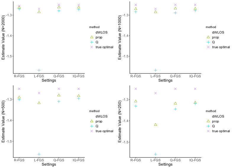
Figure S1: Value functions for estimated decision rules for regular case and different sample sizes.

References

• Austin (2009) Austin, P. C. (2009). Using the standardized difference to compare the prevalence of a binary variable between two groups in observational research. Communications in Statistics-Simulation and Computation 38, 1228–1234.
• Bai et al. (2013) Bai, X., Tsiatis, A. A. & O’Brien, S. M. (2013). Doubly-robust estimators of treatment-specific survival distributions in observational studies with stratified sampling. Biometrics 69, 830–839.
• Benkeser et al. (2017) Benkeser, D., Carone, M., van der Laan, M. & Gilbert, P. (2017). Doubly robust nonparametric inference on the average treatment effect. Biometrika 104, 863–880.
• Berk et al. (2013) Berk, R., Brown, L., Buja, A., Zhang, K., Zhao, L. et al. (2013). Valid post-selection inference. Annals of Statistics 41, 802–837.
• Butler et al. (2018) Butler, E. L., Laber, E. B., Davis, S. M. & Kosorok, M. R. (2018). Incorporating patient preferences into estimation of optimal individualized treatment rules. Biometrics 74, 18–26.
• Cao et al. (2009) Cao, W., Tsiatis, A. A. & Davidian, M. (2009). Improving efficiency and robustness of the doubly robust estimator for a population mean with incomplete data. Biometrika 96, 723–734.
• Chakraborty et al. (2013) Chakraborty, B., Laber, E. B. & Zhao, Y. (2013). Inference for optimal dynamic treatment regimes using an adaptive m-out-of-n bootstrap scheme. Biometrics 69, 714–723.
• Chakraborty & Moodie (2013) Chakraborty, B. & Moodie, E. (2013). Statistical Methods for Dynamic Treatment Regimes. Springer: New York.
• Chernozhukov et al. (2018) Chernozhukov, V., Chetverikov, D., Demirer, M., Duflo, E., Hansen, C., Newey, W. & Robins, J. (2018). Double/debiased machine learning for treatment and structural parameters. The Econometrics Journal 21, c1 – c68.
• Davidian et al. (2016) Davidian, M., Tsiatis, A. & Laber, E. (2016). Dynamic treatment regimes. In Cancer Clinical Trials: Current and Controversial Issues in Design and Analysis, S. George, X. Wang & H. Pang, eds., chap. 13. CRC Press, pp. 409–446.
• Dudoit & van der Laan (2003) Dudoit, S. & van der Laan, M. J. (2003). Asymptotics of cross-validated risk estimation in model selection and performance assessment. Tech. rep., Division of Biostatistics, University of California at Berkeley. Working Paper 126.
• Ertefaie et al. (2016) Ertefaie, A., Shortreed, S. & Chakraborty, B. (2016). Q-learning residual analysis: application to the effectiveness of sequences of antipsychotic medications for patients with schizophrenia. Statistics in Medicine 35, 2221–2234.
• Fithian et al. (2014) Fithian, W., Sun, D. & Taylor, J. (2014). Optimal inference after model selection. ArXiv:1410.2597.
• Hastie (2019) Hastie, T. (2019). gam: Generalized Additive Models. R package version 1.16.1.
• Kang et al. (2007) Kang, J. D., Schafer, J. L. et al. (2007). Demystifying double robustness: A comparison of alternative strategies for estimating a population mean from incomplete data. Statistical Science 22, 523–539.
• Laber et al. (2014) Laber, E. B., Lizotte, D. J., Qian, M., Pelham, W. E. & Murphy, S. A. (2014). Dynamic treatment regimes: Technical challenges and applications. Electronic Journal of Statistics 8, 1225.
• Lavori & Dawson (2000) Lavori, P. W. & Dawson, R. (2000). A design for testing clinical strategies: biased adaptive within-subject randomization. Journal of the Royal Statistical Society: Series A (Statistics in Society) 163, 29–38.
• Lei et al. (2012) Lei, H., Nahum-Shani, I., Lynch, K., Oslin, D. & Murphy, S. (2012). A “SMART” design for building individualized treatment sequences. Annual Review of Clinical Psychology 8, 21–48.
• Liaw & Wiener (2002) Liaw, A. & Wiener, M. (2002). Classification and regression by randomForest. R News 2, 18–22.
• Meyer et al. (2019) Meyer, D., Dimitriadou, E., Hornik, K., Weingessel, A. & Leisch, F. (2019). e1071: Misc Functions of the Department of Statistics, Probability Theory Group (Formerly: E1071), TU Wien. R package version 1.7-2.
• Milborrow (2019) Milborrow, S. (2019). earth: Multivariate Adaptive Regression Splines. R package version 5.1.1. Derived from mda:mars by Trevor Hastie and Rob Tibshirani. Uses Alan Miller’s Fortran utilities with Thomas Lumley’s leaps wrapper.
• Moodie & Kosorok (2015) Moodie, E. E. M. & Kosorok, M. R., eds. (2015). Adaptive Treatment Strategies in Practice. ASA-SIAM Series on Statistics and Applied Mathematics. Society for Industrial and Applied Mathematics.
• Murphy (2003) Murphy, S. A. (2003). Optimal dynamic treatment regimes. Journal of the Royal Statistical Society: Series B (Statistical Methodology) 65, 331–355.
• Murphy (2005) Murphy, S. A. (2005). An experimental design for the development of adaptive treatment strategies. Statistics in Medicine 24, 1455–1481.
• Nahum-Shani et al. (2012a) Nahum-Shani, I., Qian, M., Almirall, D., Pelham, W. E., Gnagy, B., Fabiano, G. A., Waxmonsky, J. G., Yu, J. & Murphy, S. A. (2012a). Experimental design and primary data analysis methods for comparing adaptive interventions. Psychological Methods 17, 457.
• Nahum-Shani et al. (2012b) Nahum-Shani, I., Qian, M., Almirall, D., Pelham, W. E., Gnagy, B., Fabiano, G. A., Waxmonsky, J. G., Yu, J. & Murphy, S. A. (2012b). Q-learning: A data analysis method for constructing adaptive interventions. Psychological Methods 17, 478.
• Polley et al. (2019) Polley, E., LeDell, E., Kennedy, C. & van der Laan, M. (2019). SuperLearner: Super Learner Prediction. R package version 2.0-25.
• Robins et al. (1992) Robins, J. M., Mark, S. D. & Newey, W. K. (1992). Estimating exposure effects by modelling the expectation of exposure conditional on confounders. Biometrics 48, 479–495.
• Robinson (1988) Robinson, P. M. (1988). Root-n-consistent semiparametric regression. Econometrica: Journal of the Econometric Society 56, 931–954.
• Rotnitzky et al. (1998) Rotnitzky, A., Robins, J. M. & Scharfstein, D. O. (1998). Semiparametric regression for repeated outcomes with nonignorable nonresponse. Journal of the American Statistical Association 93, 1321–1339.
• Schulte et al. (2014) Schulte, P. J., Tsiatis, A. A., Laber, E. B. & Davidian, M. (2014). Q-and A-learning methods for estimating optimal dynamic treatment regimes. Statistical Science 29, 640–661.
• Scornet et al. (2015) Scornet, E., Biau, G., Vert, J.-P. et al. (2015). Consistency of random forests. Annals of Statistics 43, 1716–1741.
• Shi et al. (2018) Shi, C., Fan, A., Song, R., Lu, W. et al. (2018). High-dimensional A-learning for optimal dynamic treatment regimes. Annals of Statistics 46, 925–957.
• Simoneau et al. (2018) Simoneau, G., Moodie, E. E., Platt, R. W. & Chakraborty, B. (2018). Non-regular inference for dynamic weighted ordinary least squares: understanding the impact of solid food intake in infancy on childhood weight. Biostatistics 19, 233–246.
• Song et al. (2015) Song, R., Kosorok, M., Zeng, D., Zhao, Y., Laber, E. & Yuan, M. (2015). On sparse representation for optimal individualized treatment selection with penalized outcome weighted learning. Stat 4, 59–68.
• Tsiatis (2007) Tsiatis, A. (2007). Semiparametric theory and missing data. Springer Series in Statistics. Springer: New York.
• van der Laan (2014) van der Laan, M. J. (2014). Targeted estimation of nuisance parameters to obtain valid statistical inference. The International Journal of Biostatistics 10, 29–57.
• van der Laan & Dudoit (2003) van der Laan, M. J. & Dudoit, S. (2003). Unified cross-validation methodology for selection among estimators and a general cross-validated adaptive epsilon-net estimator: Finite sample oracle inequalities and examples. Tech. rep., Division of Biostatistics, University of California at Berkeley. Working Paper 130.
• van der Laan et al. (2007) van der Laan, M. J., Polley, E. C. & Hubbard, A. E. (2007). Super learner. Statistical Applications in Genetics and Molecular Biology 6.
• van der Laan & Robins (2003) van der Laan, M. J. & Robins, J. M. (2003). Unified Methods for Censored Longitudinal Data and Causality. Springer Series in Statistics. Springer: New York.
• van der Vaart et al. (2006) van der Vaart, A. W., Dudoit, S. & van der Laan, M. J. (2006). Oracle inequalities for multi-fold cross validation. Statistics & Decisions 24, 351–371.
• Vermeulen & Vansteelandt (2015) Vermeulen, K. & Vansteelandt, S. (2015). Bias-reduced doubly robust estimation. Journal of the American Statistical Association 110, 1024–1036.
• Vermeulen & Vansteelandt (2016) Vermeulen, K. & Vansteelandt, S. (2016). Data-adaptive bias-reduced doubly robust estimation. The International Journal of Biostatistics 12, 253–282.
• Wallace & Moodie (2015) Wallace, M. P. & Moodie, E. E. (2015). Doubly-robust dynamic treatment regimen estimation via weighted least squares. Biometrics 71, 636–644.
• Watkins & Dayan (1992) Watkins, C. J. & Dayan, P. (1992). Q-learning. Machine Learning 8, 279–292.
• Zhang et al. (2012) Zhang, B., Tsiatis, A. A., Laber, E. B. & Davidian, M. (2012). A robust method for estimating optimal treatment regimes. Biometrics 68, 1010–1018.
• Zhang et al. (2013) Zhang, B., Tsiatis, A. A., Laber, E. B. & Davidian, M. (2013). Robust estimation of optimal dynamic treatment regimes for sequential treatment decisions. Biometrika 100, 681–694.
• Zhao et al. (2009) Zhao, Y., Kosorok, M. R. & Zeng, D. (2009). Reinforcement learning design for cancer clinical trials. Statistics in Medicine 28, 3294–3315.
• Zhao et al. (2012) Zhao, Y., Zeng, D., Rush, A. J. & Kosorok, M. R. (2012). Estimating individualized treatment rules using outcome weighted learning. Journal of the American Statistical Association 107, 1106–1118.
• Zhao et al. (2011) Zhao, Y., Zeng, D., Socinski, M. A. & Kosorok, M. R. (2011). Reinforcement learning strategies for clinical trials in nonsmall cell lung cancer. Biometrics 67, 1422–1433.
• Zhao et al. (2015) Zhao, Y.-Q., Zeng, D., Laber, E. B. & Kosorok, M. R. (2015). New statistical learning methods for estimating optimal dynamic treatment regimes. Journal of the American Statistical Association 110, 583–598.