A Hybrid-Order Distributed SGD Method for Non-Convex Optimization to Balance Communication Overhead, Computational Complexity, and Convergence Rate

Abstract

In this paper, we propose a method of distributed stochastic gradient descent (SGD), with low communication load and computational complexity, and still fast convergence. To reduce the communication load, at each iteration of the algorithm, the worker nodes calculate and communicate some scalers, that are the directional derivatives of the sample functions in some pre-shared directions. However, to maintain accuracy, after every specific number of iterations, they communicate the vectors of stochastic gradients. To reduce the computational complexity in each iteration, the worker nodes approximate the directional derivatives with zeroth-order stochastic gradient estimation, by performing just two function evaluations rather than computing a first-order gradient vector. The proposed method highly improves the convergence rate of the zeroth-order methods, guaranteeing order-wise faster convergence. Moreover, compared to the famous communication-efficient methods of model averaging (that perform local model updates and periodic communication of the gradients to synchronize the local models), we prove that for the general class of non-convex stochastic problems and with reasonable choice of parameters, the proposed method guarantees the same orders of communication load and convergence rate, while having order-wise less computational complexity. Experimental results on various learning problems in neural networks applications demonstrate the effectiveness of the proposed approach compared to various state-of-the-art distributed SGD methods.

1 Introduction

Stochastic gradient descent (SGD) is an optimization tool which is widely used for solving many machine learning problems, due to its simplicity and acceptable empirical performance (Rakhlin et al., 2011; Bottou, 2010). It iteratively updates the model parameters at the opposite direction of the stochastic gradient of the cost function. With the emergence of large-scale machine learning models such as deep neural networks (DNNs), however, centralized deployment of SGD has become intractable in its memory and time requirements. As such, and accelerated with the recent advances in multi-core parallel processing technology, distributed deployment of SGD has become a trend, which trains machine learning models on multiple computation nodes (a.k.a., worker nodes) in parallel, to enhance the scalability of the training procedure (Meng et al., 2019; Zinkevich et al., 2010). Under a distributed SGD method, at each iteration, each worker node evaluates a stochastic estimation of the gradient of the objective function over a randomly chosen/arrived data sample. The workers then broadcast their gradient updates to their peers, and aggregate the gradients to update the model in parallel.

Some of the major factors in designing distributed SGD algorithms, which are in conflict with each other and need to be addressed carefully, can be identified as follows:

1- Communication overhead: Distributed implementation of SGD algorithms mainly suffers from high level of communication overhead due to exchanging the stochastic gradient vectors among the worker nodes at each iteration, especially when the dimension of the model is large. In fact, the communication overhead has been observed to be the major bottleneck in scaling distributed SGD, and the time required to exchange this information will increase the overall time required for the algorithm to converge (Zhou & Cong, 2019; Alistarh et al., 2017; Strom, 2015; Chilimbi et al., 2014). As such, alleviating the communication cost has recently gained lots of attention from different research communities.

To address the issue of communication overhead, two main approaches can be identified in the literature: 1- Reducing the number of rounds of communication among the worker nodes by allowing them to perform local model updates at each iteration, and limiting their synchronization to a periodic exchange of local models after some iterations. This approach is often referred to as model averaging (McDonald et al., 2010; Zinkevich et al., 2010; Zhang et al., 2016; Su & Chen, 2015; Zhang et al., 2015; Povey et al., 2014; Kamp et al., 2018; Wang & Joshi, 2018; Zhou & Cong, 2017), 2- Reducing the number of bits communicated among the worker nodes by compression or quantization of the gradient vectors (Alistarh et al., 2017; Wen et al., 2017; Dean et al., 2012; Abadi et al., 2016; Yu et al., 2014; De Sa et al., 2015). This approach propagates the quantization error through the iterations, reduces the convergence rate, and would add to the computational complexity of each iteration.

2- Computation load: In many practical applications, the worker nodes are generally commodity devices with limited computational resources. Therefore, in order to guarantee a scalable solution, the distributed algorithm should essentially impose as low computational cost per worker node as possible.

Note that in general, one of the major derives for the computational load in SGD algorithms is the calculation of the first-order gradients at each iteration, which is very expensive, if not impossible, to obtain in many real-world problems (especially for learning large-scale models) (Hajinezhad et al., 2017). In many applications, calculating the stochastic gradient requires extensive simulation for each worker node, where the complexity of each simulation may require significant computational time (Fu, 2015). Moreover, in many scenarios of training DNNs, there is a highly complicated relationship between the parameters of the model and the objective function, so that deriving explicit form of the gradient is impossible and computing the gradient at each iteration costs significantly high computational complexity for the worker node (Lian et al., 2016).

We note that a promising approach to reduce the computational load of SGD methods is utilizing zeroth-order (ZO) gradient estimations instead of deriving the first-order gradients. In fact, since calculating a ZO gradient requires just two function evaluations (Sahu et al., 2019; Ji et al., 2019), it highly reduces the computational cost compared to the calculation of a first-order gradient (which imposes $\mathcal{O}\left(d\right)$ times higher computational complexity in general (Nesterov & Spokoiny, 2017)). Furthermore, by using pre-shared seeds for the generation of the random directions involved in zeroth-order gradients calculation, the worker nodes will not need to communicate the whole ZO gradient vectors, and can send just the scalar values of the computed derivative approximations, as will be shown in Section 3. As such, the communication overhead is significantly reduced as compared to the communication overhead imposed by sending the whole gradient vectors, especially when the dimension of the problem is large. However, loosing accuracy in calculating the gradients directly reflects in the convergence rates of zeroth-order SGD methods, especially for non-convex problems (e.g., see the convergence rates comparison in Table 1). This is one of the main challenges that we overcome in this work.

3- Convergence rate: Finally achieving fast convergence to the solution of a problem is essentially desired, especially for large-scale problems dealing with huge datasets.

1.1 Main Contributions

In this work, we propose a distributed optimization method that strikes a better balance between communication efficiency, computation efficiency and accuracy, compared to various distributed methods. The proposed methods enjoys the low computational complexity and communication overhead of the zeroth-order gradient calculation, and at the same time, benefits from periodic first-order gradient calculation and model updating. We theoretically prove that by proper combining of these two, we can achieve very good convergence rate as well. The main contributions of this work can be summarized as follows:

Table 1: Comparison of the proposed method to various state-of-the-art methods in the literature.

Method	Convergence Order	Communication Load per Iteration	Normalized Computational Load	Comments
Proposed	$\mathcal{O}(\frac{d}{\sqrt{mN}}),\text{If}~{}\tau>1$ $\mathcal{O}(\frac{1}{\sqrt{mN}}),\text{If}~{}\tau=1$	$\frac{\tau-1+d}{\tau}$	$\simeq\frac{1}{\tau}+\frac{1}{d}$
RI-SGD (Haddadpour et al., 2019)	$\mathcal{O}(\frac{\tau}{\sqrt{mN}})$	$\frac{d}{\tau}$	$\mu m+1$	requires high storage, $\mu$: redundancy factor
syncSGD (Wang & Joshi, 2018)	$\mathcal{O}(\frac{1}{\sqrt{mN}})$	$d$	$1$
ZO-SGD (Sahu et al., 2019)	$\mathcal{O}(\frac{(d/m)^{1/3}}{(N)^{1/4}})$	$1$	$\simeq\frac{1}{d}$
ZO-SVRG-Ave (Liu et al., 2018)	$\mathcal{O}(\frac{d}{N}+\frac{1}{\min{\{d,m\}}})$	$1$	$\mathcal{O}(\frac{K}{d})$	requires dataset storage, $K$: size of dataset
QSGD (Alistarh et al., 2017)	$\mathcal{O}(\frac{1}{N}+\sqrt{d})$	$\mathcal{O}(s^{2}+s\sqrt{d})$	$>1$	$s$: num. of quantization levels

• We develop a new distributed SGD method, with low communication overhead and computational complexity, and yet fast convergence. To reduce the communication load, at each iteration of the algorithm, the worker nodes calculate and communicate some scalers, that are the directional derivatives of the sample functions in some pre-shared directions. To reduce the computational complexity, the worker nodes approximate the directional derivatives with zeroth-order stochastic gradient estimation, by performing just two function evaluations. Finally, to alleviate the approximation error of the zeroh-order stochastic gradient estimations, after every $\tau\in\mathbb{N}$ iterations, the worker nodes compute and communicate the first-order stochastic gradient vectors.

• We provide theoretical analyses for the convergence rate guarantee of the proposed method. In particular, we prove that for the general class of non-convex stochastic problems, the proposed scheme converges to a stationary point with the rate of $\mathcal{O}(d/\sqrt{mN})$, which highly outperforms the convergence rates of zeroth-order methods (e.g., see (Sahu et al., 2019; Liu et al., 2018)). Moreover, compared to the fastest first-order communication-efficient algorithms (e.g., the model averaging scheme in (Haddadpour et al., 2019) with the convergence rate of $\mathcal{O}(\frac{\tau}{\sqrt{mN}})$), the proposed algorithm exhibits the same convergence rate in terms of both the number of iterations and the number of worker nodes. Finally, by a reasonable choice of $\tau=\mathcal{O}\left(d\right)$, we can guarantee the same-order communication load and convergence rate as in the fastest converging model averaging methods, with order-wise less computational complexity (see Table 1).

• Due to utilizing zeroth-order stochastic gradient updates, the proposed algorithm exhibits a sufficiently low level of computational complexity, which is much lower than the one in the communication-efficient methods including the model averaging schemes (e.g., (Haddadpour et al., 2019; Wang & Joshi, 2018)) or the schemes with gradients compression (e.g., (Alistarh et al., 2017)), and is comparable to the one in the existing zeroth-order stochastic optimization algorithms (e.g., (Sahu et al., 2019; Liu et al., 2018)). As a baseline, computational complexity of the proposed method is $\mathcal{O}\left(1/\tau+1/d\right)$ times the computational complexity of the model averaging schemes.

• Due to utilizing pre-shared seeds for the generation of random directions, at the iterations with zeroth-order gradient updates, the worker nodes just need to communicate a scalar rather than a $d$-dimensional vector, which drastically reduces the number of bits required for communication among the worker nodes. In particular, the proposed algorithm exhibits a communication load equal to sending $d+\tau-1$ scalar values by each worker node per $\tau$ iterations. This communication load is much lower than that of fully synchronous SGD (syncSGD) (Wang & Joshi, 2018), and is comparable to that of the communication-efficient schemes with model averaging, with a ratio of $\left(1+\tau/d\right)$.

• Using numerical experiments, we empirically demonstrate the accuracy and convergence properties of the proposed method compared to various state-of-the-art baselines.

Table 1 summarizes the comparison of the proposed method to the most related works in the literature, in terms of convergence rate, communication overhead per iteration, and computational load per iteration normalized to the computational complexity of computing a first-order stochastic gradient.

2 Related Work

As mentioned before, communication bottlenecks in distributed SGD originate from two sources that can be significant; first, the number of bits communicated at each communication round, and second, the number of rounds of communication. To tackle the first barrier, the existing works mainly try to quantize and compress the gradient vectors before communicating them (Alistarh et al., 2017; Wen et al., 2017; Dean et al., 2012; Abadi et al., 2016; Yu et al., 2014; De Sa et al., 2015). Although those methods are generally effective in reducing the number of bits communicated at each iteration, their quantization error increases the error variance of the communicated gradient vectors, leading to a slow convergence. To tackle the second source of communication overhead, the idea of model averaging has been proposed, where the worker nodes perform local updates at each iteration, and communicate their updated models after every $\tau$ iterations to periodically synchronize them (McDonald et al., 2010; Zinkevich et al., 2010; Zhang et al., 2016; Su & Chen, 2015; Zhang et al., 2015; Povey et al., 2014; Kamp et al., 2018; Wang & Joshi, 2018; Zhou & Cong, 2017). In consequence, the number of rounds of communication is significantly reduced.

There exist various model averaging schemes in the literature. (McMahan et al., 2016) investigated periodic averaging SGD (PA-SGD), where the models are averaged across the nodes afters every $\tau$ local updates. (Wang & Joshi, 2018) demonstrated that the convergence error of PA-SGD grows linearly in the number of local updates $\tau$. (Yu et al., 2019) provided some theoretical studies on why SGD with model averaging works well. Moreover, (Zhang et al., 2015) proposed elastic averaging SGD (EASGD), where a more complicated averaging is done by encompassing an auxiliary variable to allow some slackness between the models. They empirically validated the effectiveness of EASGD, without providing any convergence analysis. Furthermore, (Jiang et al., 2017; Lian et al., 2017) proposed consensus-based distributed SGD (D-PSGD), in which worker nodes synchronize their local models only with their neighboring nodes. By incorporating extra memory as well as high storage, (Haddadpour et al., 2019) infuse redundancy to the training data to further reduce the residual error in local averaging, and improve the convergence rate. However, this method needs more storage per worker node, and the data at different worker nodes are overlapping.

Finally, note that a key feature for both the aforementioned communication-efficient approaches is that they require stochastic first-order gradient information at each iteration (via subsequent calls to a stochastic first-order oracle (SFO)), in order to guarantee the convergence. However, as illustrated before, in many real-world applications and scenarios, it may be computationally costly for the worker nodes to obtain such information at every iteration (Hajinezhad et al., 2017). Therefore, although the approaches mentioned above provide communication-efficient solutions to distributed learning, their computational complexity may not be tolerable for general commodity worker nodes, and restricts the applicability of such methods, in practice.

To reduce the computational load of SGD methods, the idea of zeroth-order gradient estimations can be utilized. This idea has been widely used for gradient-free optimization where the explicit expressions of gradients of the objective function are expensive or infeasible to obtain, and only function evaluations are accessible (Sahu et al., 2019; Ji et al., 2019). As earlier discussed in the Introduction section, ZO gradient estimation can highly reduce the communication overhead as well as the computational complexity. However, the aforementioned benefits of zeroth-order SGD methods comes at the cost of significantly deteriorated convergence rates. This is because a zeroth-order gradient is in fact a biased estimation of the true gradient, and the involved approximation error leads to a high residual error and consequently, inferior convergence rates in zeroth-order SGD algorithms (Nesterov & Spokoiny, 2017). For example, for general non-convex problems, the (centralized) zeroth-order SGD algorithm proposed in (Sahu et al., 2019) has a convergence rate of $\mathcal{O}(\frac{d^{1/3}}{m^{1/3}N^{1/4}})$ (where $m$ denotes the number of sampled directions at each iteration of the algorithm, and hence, can be considered as equivalent to the number of worker nodes for a distributed setting).

By incorporating multiple restarts and extra memory, (Liu et al., 2018) proposed a zeroth-order extension of stochastic variance reduced gradient method (SVRG) and proved that their proposed zeroth-order SVRG (ZO-SVRG-Ave) achieves a convergence rate of $\mathcal{O}(\frac{d}{N}+\frac{1}{\min{\{d,m\}}})$ for non-convex problems, in which the second term highly deteriorates the convergence performance of the algorithm. To eliminate this error term, they proposed a coordinate-wise version of ZO-SVRG, but it costs $\mathcal{O}(d)$ times more function evaluations per iteration, which causes high computational complexity, especially for high-dimensional problems. Moreover, both of their proposed ZO-SVRG methods required full dataset storage, which is not affordable for distributed deployment on commodity devices. Furthermore, (Gao et al., 2018) proposed a zeroth-order version of the stochastic alternating direction method of multipliers with a guaranteed convergence rate of $\mathcal{O}(1/\sqrt{N})$ for convex problems but cannot be applied to general non-convex problems. We note that the slow convergence of zeroth-order stochastic gradient methods, especially for non-convex problems, is one of the main challenges that we address in this paper.

3 Communication-Efficient Distributed Stochastic Optimization Algorithm

3.1 Problem Definition

Consider a setting with $m$ distributed worker nodes that are interested in solving the following non-convex stochastic optimization problem in a distributed manner:

$$\min_{\boldsymbol{x}\in\mathbb{R}^{d}}f\left(\boldsymbol{x}\right)=\min_{\boldsymbol{x}\in\mathbb{R}^{d}}\mathbb{E}_{\boldsymbol{\zeta}}\left[F\left(\boldsymbol{x},\boldsymbol{\zeta}\right)\right],$$ (1)

where $f$ is a generic non-convex loss function, and $\boldsymbol{\zeta}$ is a random variable with unknown distribution. As a special case of the above formulation, consider the following non-convex sum problem which appears in a variety of machine learning applications, ranging from generalized linear models to deep neural networks:

$$\min_{\boldsymbol{x}\in\mathbb{R}^{d}}f\left(\boldsymbol{x}\right)=\min_{\boldsymbol{x}\in\mathbb{R}^{d}}\dfrac{1}{K}\sum_{k=1}^{K}F\left(\boldsymbol{x},\boldsymbol{\zeta}_{k}\right),$$ (2)

in which $F\left(\boldsymbol{x},\boldsymbol{\zeta}_{k}\right)$ is the training loss over the sample $\boldsymbol{\zeta}_{k}$, and $K$ is the total number of samples. Note that for generality, in the rest of this paper, we focus on the problem formulation (1). However, our analyses apply equally to both objectives.

3.2 The Proposed Algorithm

In the proposed algorithm, named as Hybrid-Order Distributed SGD (HO-SGD), at each iteration $t$, each worker node $i$ samples or receives data sample $\boldsymbol{\zeta}_{t+1,i}$ identically and independently from the dataset. Then, the data sample is used to evaluate a stochastic zeroth-order gradient approximation via computing a finite difference using two function queries as follows (Liu et al., 2018; Gao et al., 2018).

$$\tilde{\boldsymbol{G}}_{t,i}=\dfrac{d}{\mu}\Bigg{[}F\left(\boldsymbol{x}^{t}+\mu\boldsymbol{v}_{t+1,i},\boldsymbol{\zeta}_{t+1,i}\right)-F\left(\boldsymbol{x}^{t},\boldsymbol{\zeta}_{t+1,i}\right)\Bigg{]}\boldsymbol{v}_{t+1,i},$$

where $d$ is the dimension of the model to be learned, $\mu>0$ is a smoothing parameter, and $\boldsymbol{v}_{t+1,i}$ is a direction randomly drawn from a uniform distribution over a unit sphere.

Next, each worker node $i$ communicates its computed zeroth-order gradient to the other nodes. For this purpose, note that the direction of the derivatives, i.e., the vectors $\boldsymbol{v}_{t+1,i},~{}\forall i$, are some randomly generated directions, where the seeds are pre-shared among the nodes before optimization. As such, each worker node $i$ does not need to send the vector and just needs to send the value of the finite-difference approximated directional derivative, i.e., the scalar $\dfrac{d}{\mu}\left[F\left(\boldsymbol{x}^{t}+\mu\boldsymbol{v}_{t+1,i},\boldsymbol{\zeta}_{t+1,i}\right)-F\left(\boldsymbol{x}^{t},\boldsymbol{\zeta}_{t+1,i}\right)\right]$. Therefore, instead of communicating a $d$-dimensional gradient vector, each node communicates just a single scalar. As a result, the communication load reduces to $d$ times less than the communication load of exchanging the stochastic gradient vector. The model is then updated by each worker node in parallel, using the average of the local zeroth-order gradients of all the nodes, as shown by (5)-(6).

Finally, after every $\tau-1$ iterations, the worker nodes perform one iteration of first-order stochastic gradient computation and communication, and update the model accordingly. The pseudo-code of the proposed algorithm is shown in Algorithm 1. We note that the introduced algorithm does not necessarily assume that each worker node has access to the entire data. Rather, as long as each data sample is assigned to each worker node uniformly at random, Algorithm 1 works, and all the results apply.

3.3 Discussion on the Proposed Algorithm and Comparison to the Related Works

In the following, we review some remarks regarding Algorithm 1. First, note that if we choose $\tau=1$, Algorithm 1 reduces to fully synchronous distributed SGD method (Wang & Joshi, 2018; Dekel et al., 2012), where the workers perform first-order gradient computation and communication at all iterations. Moreover, if we consider $\tau\geq N$, the workers always perform zeroth-order gradient updates, thereby the algorithm reduces to distributed zeroth-order stochastic gradient method. Therefore, as the two ends of its spectrum, the proposed algorithm encompasses both zeroth-order and first-order distributed SGD algorithms as special cases.

Algorithm 1 Hybrid-Order Distributed SGD Algorithm

  Input: Dimension $d$, the total number of iterations $N$, the number of workers $m$, period $\tau\in\mathbb{N}$, smoothing parameter $\mu$, batch size $B$, initial point $\boldsymbol{x}^{0}$, step-size rule $\left\{\alpha_{t}\right\}_{t=0}^{N-1}$.

  for $t=0,\ldots,N-1$  do

     parallel for $i=1,\ldots,m$ do

         $i$-th worker receives a batch of i.i.d. samples $\left\{\boldsymbol{\zeta}_{t+1,i,b}\right\}_{b=1,\ldots,B}$.    

     if $\mod(t,\tau)=0$ then

            $i$-th worker computes the first-order stochastic gradient vector, as follows:

$$\tilde{\boldsymbol{G}}_{t,i}\leftarrow \dfrac{1}{B}\sum_{b=1}^{B}\nabla F\left(\boldsymbol{x}^{t},\boldsymbol{\zeta}_{t+1,i,b}\right)$$ (3)

   

     else

            $i$-th worker picks a direction $\boldsymbol{v}_{t+1,i}$ uniformly at random from the unit sphere, and computes a zeroth-order stochastic gradient as follow:

$$\tilde{\boldsymbol{G}}_{t,i}\leftarrow\dfrac{1}{B}\sum_{b=1}^{B}\dfrac{d}{\mu}\Big{[} F\left(\boldsymbol{x}^{t}+\mu\boldsymbol{v}_{t+1,i},\boldsymbol{\zeta}_{t+1,i,b}\right)$$

$$-F\left(\boldsymbol{x}^{t},\boldsymbol{\zeta}_{t+1,i,b}\right)\Big{]}\boldsymbol{v}_{t+1,i}$$ (4)

   

     end if

     

$$\tilde{\boldsymbol{G}}_{t}=\dfrac{1}{m}\sum_{i=1}^{m}\tilde{\boldsymbol{G}}_{t,i}$$ (5)

$$\boldsymbol{x}^{t+1}=\boldsymbol{x}^{t}-\alpha_{t}\tilde{\boldsymbol{G}_{t}}$$ (6)

     end parallel for

  end for

  Output: $\boldsymbol{x}^{N}$.

To address the challenge of slow convergence of zeroth-order SGD iterations, the proposed method employs periodic rounds of first-order stochastic gradient updates. This significantly reduces the residual error of the zeroth-order stochastic gradient updates, as compared to the existing zeroth-order methods. Therefore, our algorithm can be viewed as a zero-order stochastic optimization with periodic rounds of first-order updates, which reduces the communication overhead and computational complexity, and at the same time guarantees improved convergence rate (as will be seen in the next section). In particular, the main advantages of the proposed algorithm can be identified as follows:

Low computational complexity: By employing zeroth-order stochastic gradient estimations, each worker node performs just two function evaluations, rather than a gradient computation. This contributes to a significant reduction in the computational complexity of the proposed algorithm, as compared to the previous first-order distributed methods. In particular, it is estimated that in general, computing a zeroth-order gradient estimation costs $\mathcal{O}\left(d\right)$ times less computational load than computing a first-order gradient estimation (Nesterov & Spokoiny, 2017). Therefore, considering $\tau-1$ iterations of zeroth-order update and one iteration of first-order update at each period of $\tau$ iterations of Algorithm 1, the computational complexity of the proposed algorithm is extremely lower than that of the first-order communication-efficient methods, with a ratio of $\mathcal{O}\left(\frac{1}{d}+\frac{1}{\tau}\right)$, and is comparable to the one in the distributed zeroth-order methods.

Low communication overhead: As aforementioned, due to utilizing pre-shared seeds for the generation of random directions, at the iterations with zeroth-order gradient updates, the worker nodes just need to communicate a scalar instead of a $d$-dimensional vector, which drastically reduces the number of bits required for communication. In particular, the communication overhead of the proposed scheme is $\left(1+\frac{\tau-1}{d}\right)$ times the communication overhead of the fastest first-order communication-efficient methods (i.e., model-averaging schemes such as (Haddadpour et al., 2019)), and is comparable to the communication overhead in the zeroth-order methods.

Fast convergence rate: Finally, the proposed algorithm guarantees a fast convergence rate for a general class of non-convex problems. As will be shown in the next section, in terms of the number of iterations and the number of workers, the proposed method guarantees the same convergence rate as those of the fastest first-order communication-efficient methods, and order-wisely better convergence rate than those of the zeroth-order methods.

4 Convergence Analysis

In this section, we present the convergence analysis of the proposed algorithm for a general class of non-convex problems. Prior to that, we first state the main assumptions and definitions used for the convergence analysis.

4.1 Assumptions and Definitions

Our convergence analysis is based on the following assumptions, which are all standard and widely used in the context of non-convex optimization (Meng et al., 2019).

Assumption 1 (Unbiased and finite variance first-order stochastic gradient estimation).

The stochastic gradient evaluated on each data sample $\boldsymbol{\zeta}$ by the first-order oracle is an unbiased estimator of the full (exact) gradient, i.e.,

$$\mathbb{E}\left[\nabla F\left(\boldsymbol{x},\boldsymbol{\zeta}\right)\right]=\nabla f\left(\boldsymbol{x}\right),~{}~{}\forall\boldsymbol{x}\in\mathbb{R}^{d},$$ (7)

with a finite variance, i.e., there exists a constant $\sigma\leq 0$ such that

$$\mathbb{E}\left[\parallel\nabla F\left(\boldsymbol{x},\boldsymbol{\zeta}\right)-\nabla f\left(\boldsymbol{x}\right)\parallel^{2}\right]\leq\sigma^{2},~{}~{}\forall\boldsymbol{x}\in\mathbb{R}^{d}.$$ (8)

Assumption 2 (Lipschitz continuous and bounded gradient).

The objective function $isf\left(\boldsymbol{x}\right)$ is differentiable and $L$-smooth, i.e., its gradient $\nabla f$ is $L$-Lipschitz continuous:

$$\parallel\nabla f\left(\boldsymbol{x}\right)-\nabla f\left(\boldsymbol{y}\right)\parallel\leq L\parallel\boldsymbol{x}-\boldsymbol{y}\parallel,~{}~{}~{}\forall\boldsymbol{x},\boldsymbol{y}\in\mathbb{R}^{d}.$$ (9)

Moreover, the norm of the gradient of the objective function is bounded, i.e., there exists a constant $M\leq 0$ such that

$$\parallel\nabla f\left(\boldsymbol{x}\right)\parallel\leq M,\quad\forall\boldsymbol{x}\in\mathbb{R}^{d}.$$ (10)

Assumption 3 (Bounded bellow objective function value).

The objective function value is bounded below by a scalar $f^{\ast}$.

4.2 Main Results

First, note that since $f\left(\boldsymbol{x}\right)$ is non-convex, we need a proper measure to show the gap between the the output of the algorithm and the set of stationary solutions. As such and similar to the previous works, we consider the expected gradient norm as an indicator of convergence, and state the algorithm achieves an $\epsilon$-suboptimal solution if (Bottou et al., 2018):

$$\mathbb{E}\left[\dfrac{1}{N}\sum_{t=1}^{N}\parallel\nabla f\left(\boldsymbol{x}^{t}\right)\parallel^{2}\right]\leq\epsilon.$$ (11)

Noted that this condition guarantees convergence of the algorithm to a stationary point (Wang & Joshi, 2018).

The following theorem presents the main convergence result of the proposed algorithm. Note that all the intermediate results and analytical proofs have been deferred to Appendix Appendix B.

Theorem 1 (Convergence of the proposed method).

In the proposed Algorithm 1, under Assumptions 1-3, if the step-size (a.k.a., the learning rate) and the smoothing parameter are chosen such that $\alpha_{t}=\frac{\sqrt{Bm}}{L\sqrt{N}},~{}\forall t$ and $\mu\leq\frac{1}{\sqrt{dN}}$, respectively, and the total iterations $N$ is sufficiently large, i.e., $N>\frac{16\left(d+Bm-1\right)^{2}}{Bm}$, then the average-squared gradient norm after $N$ iterations is bounded by:

$$\dfrac{1}{N} \sum_{t=0}^{N-1}\mathbb{E}\left[\parallel\nabla f\left(\boldsymbol{x}^{t}\right)\parallel^{2}\right]$$ (12)

$$\leq\frac{4L\left(f\left(\boldsymbol{x}^{0}\right)-f^{\ast}\right)}{\sqrt{BmN}}+\frac{2\sigma^{2}}{\sqrt{BmN}\tau}$$

$$\quad+1\left(\tau>1\right)\Bigg{(}\frac{4L^{2}}{d^{2}\sqrt{BmN}\tau}+\frac{4L^{2}}{d^{2}N\sqrt{BmN}}$$

$$\quad+\frac{L^{2}}{\sqrt{BmN}}\frac{\tau-1}{\tau}+\frac{L^{2}}{N\sqrt{BmN}\tau}+\frac{4d\sigma^{2}}{\sqrt{BmN}}\frac{\tau-1}{\tau}$$

$$\quad+\frac{4d\sigma^{2}}{N\sqrt{BmN}\tau}+\frac{L^{2}}{\sqrt{BmN}}\dfrac{\tau-1}{\tau}+\frac{L^{2}}{N\sqrt{BmN}\tau}\Bigg{)},$$

where $\mathbf{1}(\cdot)$ is the indicator function.

Remark 1 (Order of Convergence).

The above theorem indicates that for any $\tau>1$, the convergence rate is of the order of $\left(\frac{d}{\sqrt{mN}}\frac{\tau-1}{\tau}\right)=\mathcal{O}\left(\frac{d}{\sqrt{mN}}\right)$ with respect to the parameters of the problem, which significantly outperforms the zeroth-order stochastic gradient methods (see Table 1 for more details). Moreover, by setting the period of the first-order gradient updates such that $\tau=\mathcal{O}\left(d\right)$, we can guarantee the same convergence rate as in the fastest converging communication-efficient methods such as (Haddadpour et al., 2019), which has the convergence rate of $\mathcal{O}\left(\frac{\tau}{\sqrt{mN}}\right)$. Also note that in the special case of $\tau\geq N$, i.e., when the workers only use stochastic zeroth-order oracle for gradient estimation, the proposed algorithm recovers zeroth-order SGD algorithm. In this case also, our obtained convergence rate significantly improves the previous results on the convergence rate of the zeroth-order SGD algorithms (Sahu et al., 2019; Liu et al., 2018). Finally, when $\tau=1$, i.e., when the workers only use stochastic first-order oracle for gradient estimation, the above theorem guarantees a convergence rate of $\mathcal{O}(\frac{1}{\sqrt{mN}})$, which is consistent with the convergence rate of fully synchronous SGD (Wang & Joshi, 2018), (Dekel et al., 2012).

Remark 2 (Error decomposition).

It is noted that the error upper bound (12) is decomposed into two parts. The first part, which contains the first two terms, is similar to the error bound in fully synchronous SGD (Bottou et al., 2018), and is resulted from the periodic steps of first-order stochastic gradient updates. The second part, containing the remaining terms, is a measure of the approximation error in zeroth-order stochastic gradient steps, and vanishes when $\tau=1$, i.e., when there is no zeroth-order gradient updates.

Remark 3 (Dependence on $\tau$).

It should be noted that the upper bound (12) grows very slowly with the period of first-order updates $\tau$, with an order of $\mathcal{O}\left(1\right)$. As a result, for a fixed number of iterations, our algorithm needs few rounds of first-order stochastic gradient vectors computation and communication among the nodes to reach a certain error bound. This significantly contributes to the communication efficiency and computation efficiency of the proposed algorithm. Moreover, such growth rate significantly outperforms the existing results in the model averaging schemes, where the error upper bound grows quadratically or linearly with $\tau$, which is a result of high model discrepancies due to local model updates (Yu et al., 2018; Zhou & Cong, 2017; Haddadpour et al., 2019).

5 Experiments

In this section, we experimentally evaluate the performance of the proposed algorithm and compare it to various state-of-the-art distributed algorithms, including the model averaging scheme RI-SGD (Haddadpour et al., 2019), fully synchronous SGD (syncSGD) (Wang & Joshi, 2018), zeroth-order stochastic gradient method (ZO-SGD) (Sahu et al., 2019), and the zeroth-order stochastic variance reduced gradient method (ZO-SVRG-Ave) (Liu et al., 2018). We evaluate the performance of the proposed algorithm on two different applications, as follows.

5.1 Generation of Adversarial Examples from DNNs

The first application is generation of adversarial examples from DNNs, which arises in testing the robustness of a de- ployed DNN to adversarial attacks. In the context of image classification, adversarial examples are carefully crafted perturbed images that are barely noticable and visually imperceptible, but when added to natural images, can fool the target model to mis-classify (Madry et al., 2017; Liu et al., 2018). In many applications dealing with mission-critical information, the robustness of a deployed DNN to adversarial attacks is highly critical for reliability of the model, e.g., traffic sign identification for autonomous driving. The task of generating a universal adversarial perturbation to $K$ natural images can be regarded as an optimization problem of the form (2). More details on the problem formulation of generating adversarial examples can be found in Appendix Appendix A. Note that in general, the attacker can utilize the model evaluations and the parameters of the model to acquire its gradients (Madry et al., 2017).

Experimental Setup: Similar to (Liu et al., 2018), we apply the proposed algorithm and the baselines to generate adversarial examples to attack a well-trained DNN7 on the MNIST handwritten digit classification task, which achieves 99.4 test accuracy on natural examples. In our experiments, performed on a system with an Nvidia Tesla K80 GPU, we choose $n=10$ examples from the same class, and set the batch size and the number of workers to $B=5$ and $m=5$, respectively, for all the methods. We also use a constant step-size of $30/d$, where $d=900$ is the image dimension, and the smoothing parameter follows $\mu=\mathcal{O}(1/\sqrt{dN})$, where $N$ is the number of iterations.

Experimental Results: Fig. 1 depicts the attack loss versus the number of iterations, and Table 2 shows the least $l_{2}$ distortion of the successful (universal) adversarial examples. It can be verified that compared to the zeroth-order methods of ZO-SGD and ZO-SVRG-Ave, the proposed method achieves significantly faster convergence and lower loss. Moreover, its convergence speed and attained loss is comparable to those of the fastest first-order methods, i.e., RI-SGD and Synchronous SGD. In terms of $l_{2}$ distortion, the proposed method suggests better visual quality of the resulting adversarial examples than those in the previous zeroth-order methods, and its visual quality is similar to those of the first-order methods.

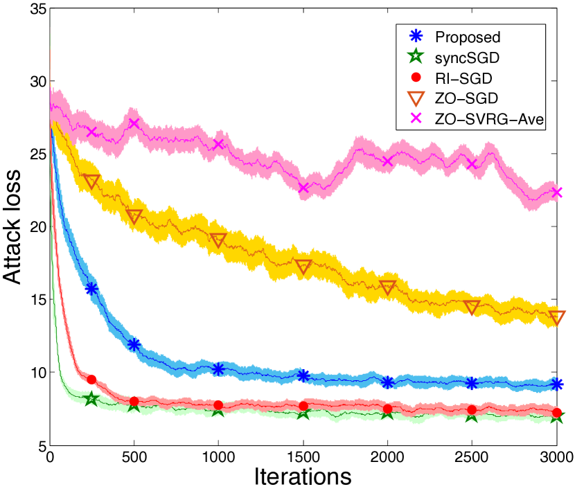
Figure 1: Comparison of different methods for the task of generating universal adversarial examples from a DNN. Attack loss versus iterations.

Table 2: $l_{2}$ distortion

Method	$l_{2}$ distortion
RI-SGD	$6.08$
syncSGD	$5.90$
Proposed	$8.86$
ZO-SGD	$10.07$
ZO-SVRG-Ave	$16.41$

Table 3 shows the original natural images along with the resulted adversarial examples generated by different methods, under the elaborated experimental setup.

Table 3: The generated adversarial examples from a well-trained DNN7 on MNIST using the proposed method and the baselines.

Image ID	6	72	128	211	315	398	475	552	637	738
Original
HO-SGD (Proposed)
Classified as	3	3	8	8	8	3	7	3	8	3
ZO-SGD
Classified as	3	8	8	8	8	8	7	3	8	3
ZO-SVRG-Ave
Classified as	8	7	8	8	8	8	7	3	8	3
syncSGD
Classified as	3	8	8	8	8	8	7	3	8	3
RI-SGD
Classified as	3	3	8	8	8	3	7	3	8	3

Table 4: Details of the datasets used in the second experiments.

Dataset	$\verb|#|$ Classes	$\verb|#|$ Training data	$\verb|#|$ Testing data	$\verb|#|$ Features	Description
SENSORLESS	$11$	$48509$	$10000$	$48$	Sensor-less drive diagnosis (Wang et al., 2018)
ACOUSTIC	$3$	$78823$	$19705$	$50$	Accoustic vehicle classification in distributed sensor networks (Duarte & Hu, 2004)
COVTYPE	$7$	$50000$	$81012$	$54$	Forest cover type prediction from cartographic variables only (Asuncion & Newman, 2007)
SEISMIC	$3$	$78823$	$19705$	$50$	Seismic vehicle classification in distributed sensor networks (Duarte & Hu, 2004)

5.2 Multi-Class Classification Tasks with Multiple Workers

The second experiment includes various multi-class classification tasks performed by multiple worker nodes in a distributed environment. We use four different famous datasets, including COVTYPE, SensIT Vehicle (both ACOUSTIC and SEISMIC), and SENSORLESS. Details and the description of each dataset can be found in Table 4.

Experimental Setup: As the base model for training, we choose a high-dimensional fully connected two-layer neural network with more than $1.69M$ parameters ($1.3K$ and $1.3K$ hidden neurons, consecutively), i.e., $d>1.69\times 10^{6}$. We use PyTorch (Paszke et al., 2019) to develop the proposed algorithm and the baselines in a distributed environment, and conduct different types of experiments on a system with 8 Cores of CPU and 4 Nvidia Tesla K80 GPUs.

The number of worker nodes and the batch size are set to $m=4$ and $B=64$, respectively, for all the methods, and the period of the first-order gradient exchanges is set to $\tau=8$ for the proposed method and the periodic model averaging method of RI-SGD. Moreover, a redundancy factor of $\mu=0.25$ is considered for the RI-SGD method. All the methods are run from the same initial points. Finally, it should be noted that for each dataset, we have optimized the learning rates of all the methods, in order to have a fair comparison.

Experimental Results: The performance of different methods in distributed training of the considered model for various datasets is compared in Fig. 2. It shows the training loss versus iterations, the training loss versus wall-clock time (in seconds), and the testing accuracy versus wall-clock time, for different datasets as aforementioned. As can be verified from the figures, the proposed method significantly outperforms the zeroth-order method ZO-SGD, in terms of convergence speed, wall-clock time, and testing accuracy. Moreover, despite the high dimension of the model, the performance of the proposed method is still comparable to the first-order methods of sync-SGD and RI-SGD (which is a model averaging method with the complementary help of infused redundancy), while the proposed method benefits from lower computational complexity as discussed before. These experimental findings comply with our theoretical results discussed in Section 4.

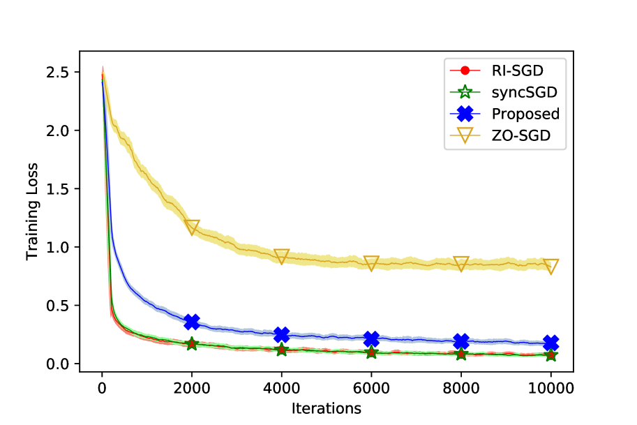
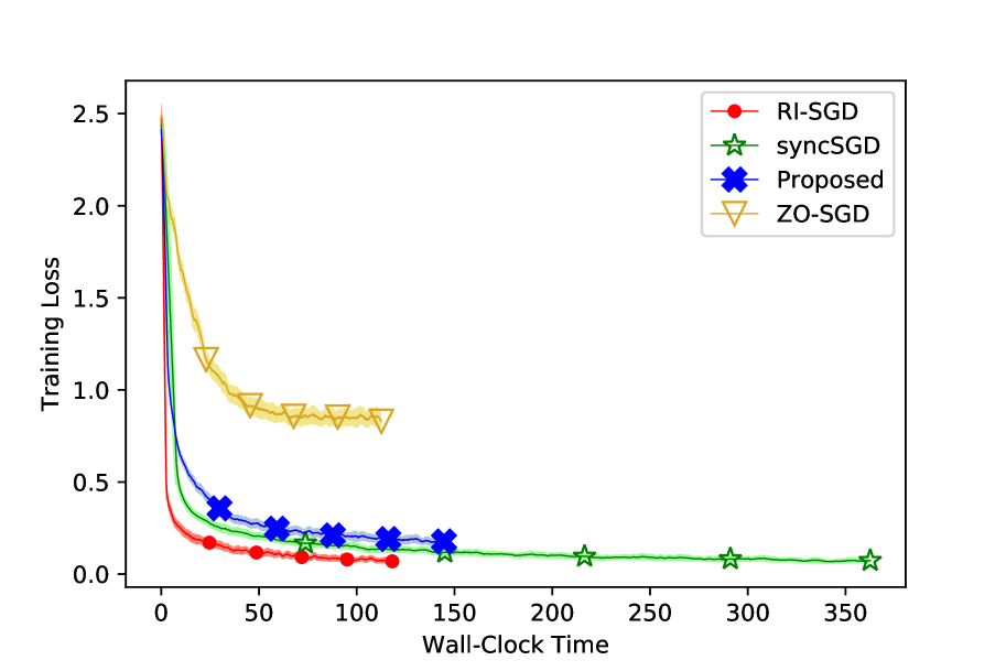
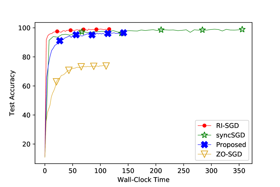
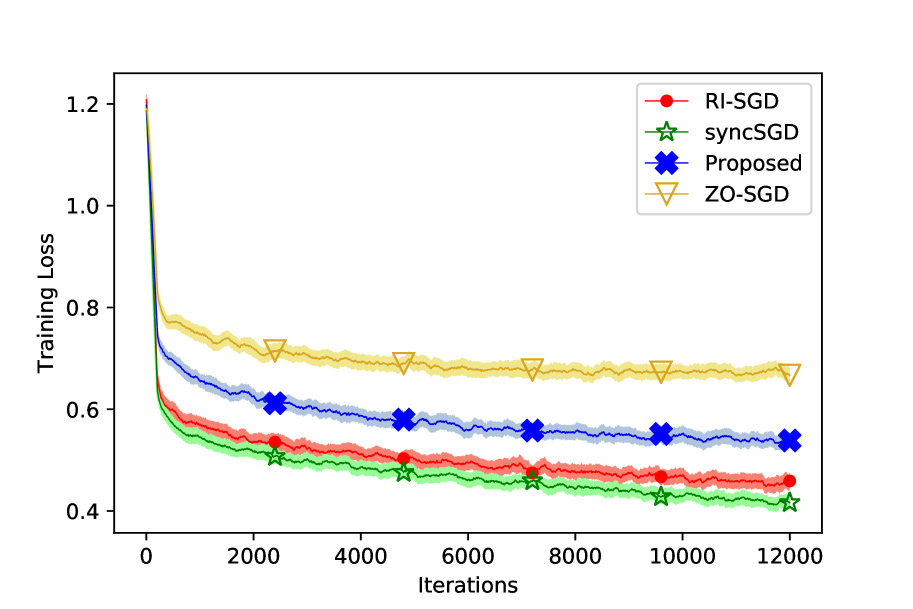
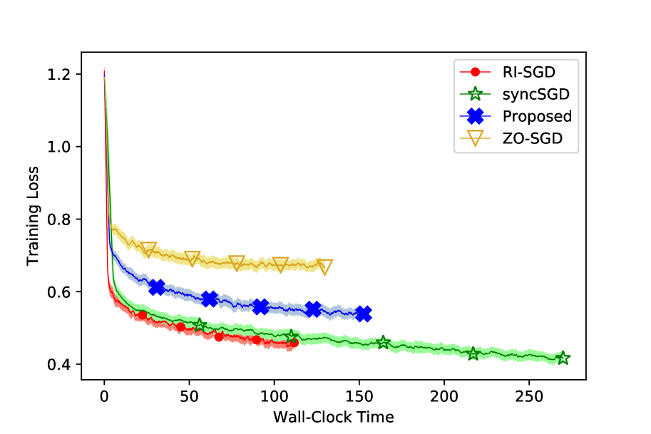
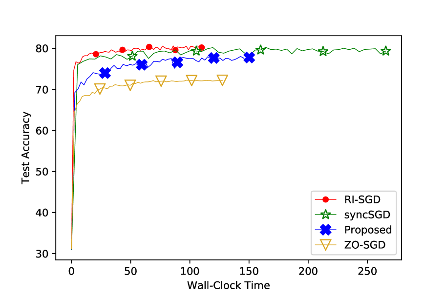
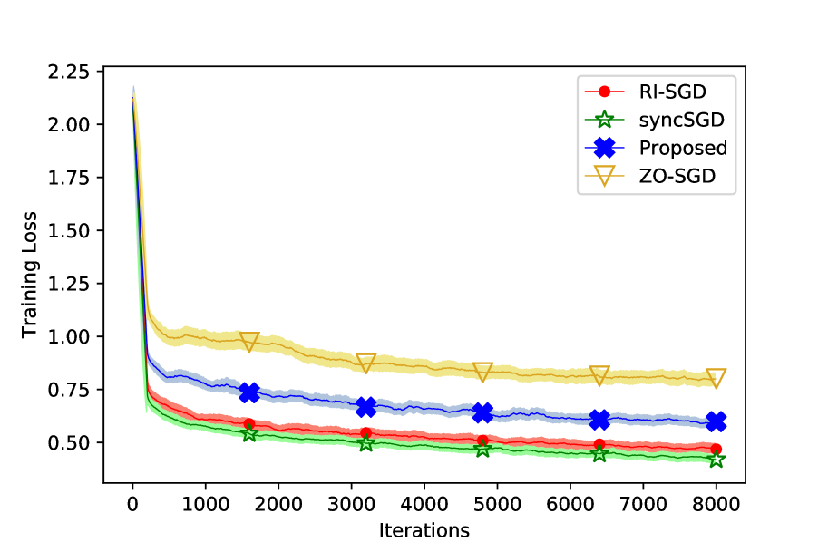
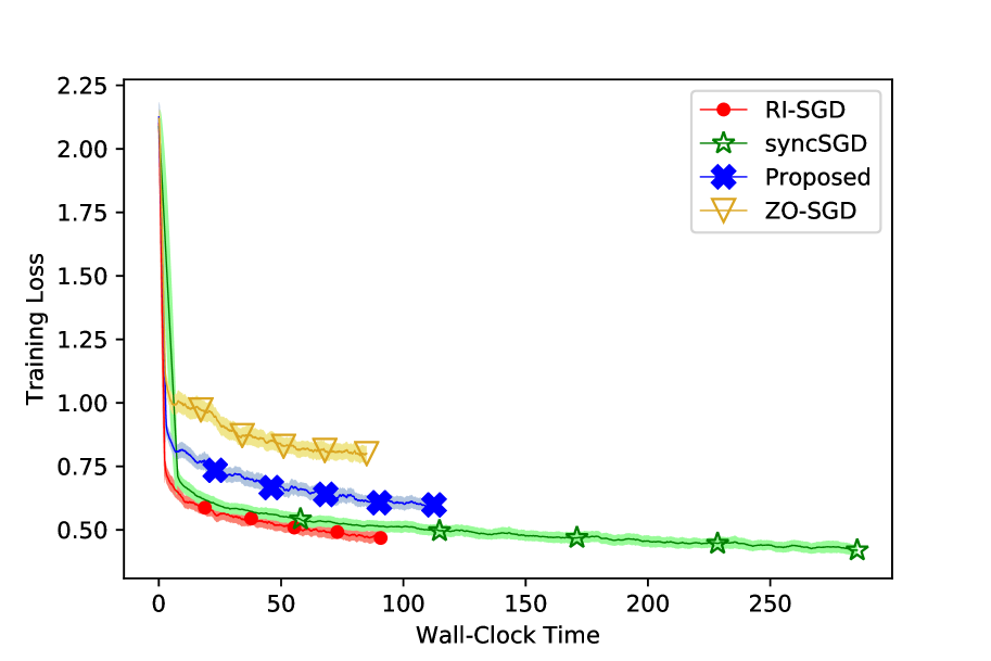
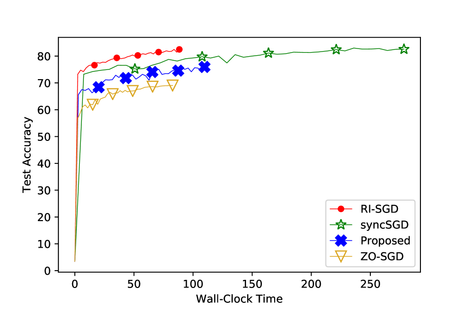
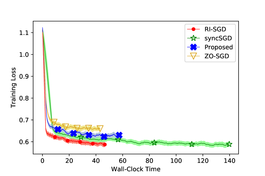
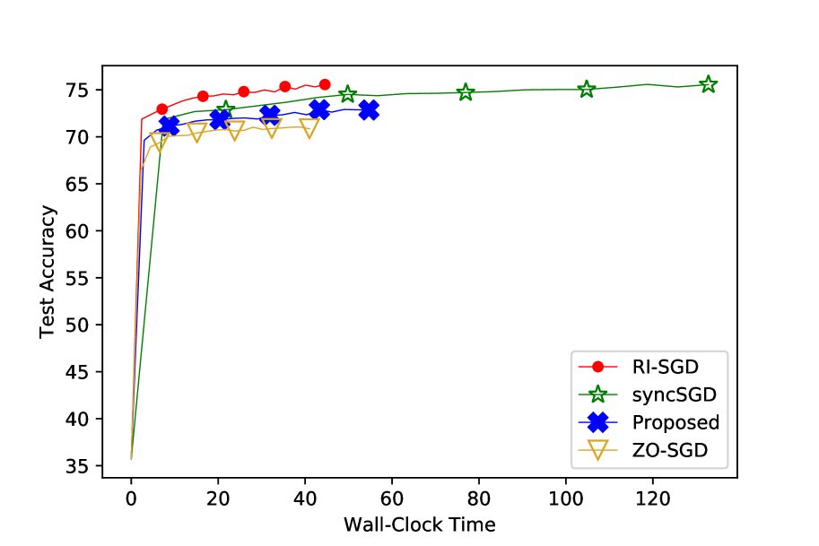
Figure 2: Training loss and test accuracy comparisons of different methods. The rows correspond to SENSORLESS, ACOUSTIC, COVTYPE, and SEISMIC datasets, from top to down, respectively. Wall-clock times are measured in seconds.

6 Conclusion

In this paper, we proposed a hybrid zeroth/first-order distributed SGD method for solving non-convex unconstrained stochastic optimization problems that benefits from low communication overhead and computational complexity, and yet converges fast. By theoretical analyses, we showed that the proposed algorithm reaches the same iteration complexity as the first-order distributed SGD algorithms, while it enjoys order-wisely lower computational complexity and comparable communication overhead. Moreover, the proposed algorithm significantly outperforms the convergence rates of the existing zeroth-order algorithms, guaranteeing a convergence rate of the order of $\mathcal{O}\left(d/\sqrt{mN}\right)$, with a comparable computational complexity. Experimental results demonstrate the effectiveness of the proposed approach compared to various state-of-the-art methods.

Appendix Appendix A Problem Formulation of Generating Adversarial Examples from DNN

Here, we elaborate the details of the problem formulation for the task of generating adversarial examples considered in Section 5.1. The task of generating a universal adversarial perturbation to $K$ natural images can be regarded as an optimization problem of the form (2), in which $F\left(\boldsymbol{x},\boldsymbol{\zeta}_{k}\right)$ is the designed attack loss function of the $k^{\text{th}}$ image, and is defined as (Carlini & Wagner, 2017)

$$F\left(\boldsymbol{x},\boldsymbol{\zeta}_{k}\right)= c.\max\left\{0,f_{y_{k}}\left(0.5\tanh\left(\tanh^{-1}2\boldsymbol{a}_{k}+\boldsymbol{x}\right)\right)-\max_{j\neq y_{j}}f_{j}\left(0.5\tanh\left(\tanh^{-1}2\boldsymbol{a}_{k}+\boldsymbol{x}\right)\right)\right\}$$

$$+\parallel 0.5\tanh\left(\tanh^{-1}2\boldsymbol{a}_{k}+\boldsymbol{x}\right)-\boldsymbol{a}_{k}\parallel^{2}_{2},$$

where $\boldsymbol{\zeta}_{k}=\left(\boldsymbol{a}_{k},y_{k}\right)$ in which, $\boldsymbol{a}_{k}\in\left[-0.5,0.5\right]^{d}$ and $y_{k}$ denote the $k^{\text{th}}$ natural image and its original class label, respectively. Furthermore, for a generated adversarial example $\boldsymbol{z}$ and for each image class $i=1,\cdots,I$, the function $f_{i}\left(\boldsymbol{z}\right)$ outputs prediction score of the model (e.g., log-probability) in that class. Note that in the above formulation, the $\tanh$ operation is used to keep the generated adversarial example, i.e., $\boldsymbol{z}=0.5\tanh\left(\tanh^{-1}2\boldsymbol{a}_{k}+\boldsymbol{x}\right)$, in the valid image space $\left[-0.5,0.5\right]^{d}$. Finally, $c$ is a regularization parameter to balance a trade-off between the adversarial attack success and the $l_{2}$ distortion of the adversarial example. Note that lower values for $c$ result in lower $l_{2}$ distortion which suggests better visual quality of the resulting adversarial examples, while higher values for $c$ results in higher success rate of the adversarial attack (i.e., it can perturb more natural images to be misclassified).

Appendix Appendix B Convergence Proofs

In order to prove Theorem 1, we first define some auxiliary variables and functions, then we present and prove some useful lemmas which will be utilized for proving Theorem 1. Note that unless stated otherwise, the expectations are with respect to all the random variables.

B.1 Preliminary Definitions

We use the following smoothing scheme to approximate the first-order information of a given function $f$.

Definition 1.

For any smoothing parameter $\mu>0$, the co-called smoothing function of any original function $f\left(\boldsymbol{x}\right)$ is defined as (Darzentas, 1984):

$$f_{\mu}\left(\boldsymbol{x}\right)\triangleq\mathbb{E}_{\boldsymbol{u}\sim U_{b}}\left[f\left(\boldsymbol{x}+\mu\boldsymbol{u}\right)\right],$$ (13)

where $U_{b}$ is the uniform distribution over the Euclidean $d$-dimensional unit ball.

The above smoothing scheme exhibits several interesting features that we shall use for the analysis of the convergence of the proposed method. For example, as shown by Lemma 4.1(b) in (Gao et al., 2018), for any function $f\in C_{L}^{1}\left(\mathbb{R}^{d}\right)$ (this condition is satisfied under (9) in Assumption 2), we have

$$|f_{\mu}\left(\boldsymbol{x}\right)-f\left(\boldsymbol{x}\right)|\leq\dfrac{\mu^{2}L}{2},$$ (14)

and

$$\parallel\nabla f_{\mu}\left(\boldsymbol{x}\right)-\nabla f\left(\boldsymbol{x}\right)\parallel\leq\dfrac{\mu Ld}{2}.$$ (15)

Definition 2.

Here, we define three functions that will be extensively used in the analysis of the proposed algorithm.

• The function $\tilde{f}_{t}\left(\boldsymbol{x}\right)$ indicates the considered function at each iteration of the proposed algorithm (that is being minimized by using its stochastic gradient direction):

  $$\tilde{f}_{t}\left(\boldsymbol{x}\right)\triangleq\left\{\begin{array}[]{ll}{f\left(\boldsymbol{x}\right)}&{\mathrm{If}\mod\left(t,\tau\right)=0,}\\ \\ {f_{\mu}\left(\boldsymbol{x}\right)}&{\mathrm{Otherwise.}}\end{array}\right.$$ (16)

• Moreover, $\tilde{\boldsymbol{G}}_{t}$ indicates the update direction, or equivalently, the gradient estimation of the objective function, utilized at each iteration of the proposed algorithm:

  $$\tilde{\boldsymbol{G}}_{t}\left(\boldsymbol{x}\right)\triangleq\left\{\begin{array}[]{ll}{\dfrac{1}{Bm}\sum_{i=1}^{m}\sum_{b=1}^{B}\nabla F\left(\boldsymbol{x},\boldsymbol{\zeta}_{t+1,i,b}\right)}&{\mathrm{If}\mod\left(t,\tau\right)=0,}\\ \\ {\dfrac{1}{Bm}\sum_{i=1}^{m}\sum_{b=1}^{B}\boldsymbol{G}_{\mu}\left(\boldsymbol{x},\boldsymbol{\zeta}_{t+1,i,b},\boldsymbol{v}_{t+1,i}\right)}&{\mathrm{Otherwise,}}\end{array}\right.$$ (17)

  where $\boldsymbol{G}_{\mu}\left(\boldsymbol{x},\boldsymbol{\zeta}_{t+1,i,b},\boldsymbol{v}_{t+1,i}\right)$ is the zeroth-order gradient estimation and is defined as

  $$\boldsymbol{G}_{\mu}\big{(}\boldsymbol{x},\boldsymbol{\zeta}_{t+1,i,b},\boldsymbol{v}_{t+1,i}\big{)}\triangleq\dfrac{d}{\mu}\Big{[}F\left(\boldsymbol{x}^{t}+\mu\boldsymbol{v}_{t+1,i},\boldsymbol{\zeta}_{t+1,i,b}\right)-F\left(\boldsymbol{x}^{t},\boldsymbol{\zeta}_{t+1,i,b}\right)\Big{]}\boldsymbol{v}_{t+1,i}.$$ (18)

• Finally, $\tilde{\boldsymbol{\delta}}_{t}$ indicates the difference between the utilized gradient estimation and the true gradient of the function considered at each iteration:

  $$\tilde{\boldsymbol{\delta}}_{t}\left(\boldsymbol{x}\right)\triangleq\nabla\tilde{f}_{t}\left(\boldsymbol{x}\right)-\tilde{\boldsymbol{G}}_{t}\left(\boldsymbol{x}\right).$$ (19)

B.2 Preliminary Lemmas

First, note that according to the definition of $\tilde{G}_{t}$ in (17) and Assumption 1, using Lemma 4.2 in (Gao et al., 2018), it can be shown that for all $t\geq 0$,

$$\mathbb{E}_{\boldsymbol{\zeta}_{t+1},\boldsymbol{v}_{t+1}}\left[\tilde{\delta}_{t}\left(\boldsymbol{x}\right)\right]=0,~{}~{}\forall\boldsymbol{x}\in\mathbb{R}^{d}.$$ (20)

In the following, some useful lemmas are in order.

Lemma 1.

For any $L$-smooth function $f\left(\boldsymbol{x}\right)$: $~{}\forall t\geq 0,~{}\forall\boldsymbol{x}\in\mathbb{R}^{d}$,

$$\tilde{f}_{t+1}\left(\boldsymbol{x}\right)\leq\left\{\begin{array}[]{ll}{\tilde{f}_{t}\left(\boldsymbol{x}\right)+\dfrac{\mu^{2}L}{2}}&{\mathrm{If}\mod\left(t+1,\tau\right)=0~{}XOR\mod\left(t,\tau\right)=0,}\\ \\ {\tilde{f}_{t}\left(\boldsymbol{x}\right)}&{\mathrm{Otherwise.}}\end{array}\right.$$ (24)

Proof.

If one and only one of $t$ and $t+1$ divides $\tau$, it can be followed that exactly one of the two functions $\tilde{f}_{t+1}\left(.\right)$ and $\tilde{f}_{t}\left(.\right)$ is $f\left(.\right)$ and the other one is $f_{\mu}\left(.\right)$. Therefore, according to (14), it can be concluded that the difference of these two functions at any point $\boldsymbol{x}\in\mathbb{R}^{d}$ is upper-bounded by $\dfrac{\mu^{2}L}{2}$. Otherwise (i.e., if both $t$ and $t+1$ divide $\tau$ or both $t$ and $t+1$ do not divide $\tau$), then according to (14), both the associated functions are the same, and hence, their difference is zero at any point $\boldsymbol{x}\in\mathbb{R}^{d}$. ∎

Remark 4.

When running Algorithm 1 for $N$ iterations ($t=0,\ldots,N-1$), it can be shown that if $\tau>1$, the first case of the above lemma occurs exactly $2\left\lfloor{\dfrac{N-1}{\tau}}\right\rfloor-1$ times. Otherwise (i.e., if $\tau=1$), the first case never occurs. This will be used later on in upper-bounding the error terms in the proof of the main theorem, i.e., Theorem 1.

Lemma 2.

For any $L$-smooth function $f\left(\boldsymbol{x}\right)$: $~{}\forall t\geq 0,~{}\forall\boldsymbol{x}\in\mathbb{R}^{d}$,

$$\parallel\nabla\tilde{f}_{t}\left(\boldsymbol{x}\right)\parallel^{2}\geq\left\{\begin{array}[]{ll}{\parallel\nabla f\left(\boldsymbol{x}^{t}\right)\parallel^{2}}&{\mathrm{If}\mod\left(t,\tau\right)=0,}\\ \\ {\dfrac{1}{2}\parallel\nabla f\left(\boldsymbol{x}^{t}\right)\parallel^{2}-\dfrac{\mu^{2}d^{2}L^{2}}{4}}&{\mathrm{Otherwise.}}\end{array}\right.$$ (28)

Proof.

For the case when $t$ satisfies $\mod\left(t,\tau\right)=0$, the result is obvious as we have $\tilde{f}_{t}\left(\boldsymbol{x}\right)=f\left(\boldsymbol{x}\right)$ (due to the definition in (16)), and hence, $\nabla\tilde{f}_{t}\left(\boldsymbol{x}\right)=\nabla f\left(\boldsymbol{x}\right)$. For the case when $\mod\left(t,\tau\right)\neq 0$, starting from (15) and using the fact that $\parallel\boldsymbol{a}\parallel^{2}\leq 2\parallel\boldsymbol{b}\parallel^{2}+2\parallel\boldsymbol{a}-\boldsymbol{b}\parallel^{2},~{}\forall\boldsymbol{a},\boldsymbol{b}\in\mathbb{R}^{d}$, we have

$$\parallel\nabla f\left(\boldsymbol{x}\right)\parallel^{2} \leq 2\parallel\nabla\tilde{f}_{t}\left(\boldsymbol{x}\right)\parallel^{2}+\parallel\nabla\tilde{f}_{t}\left(\boldsymbol{x}\right)-\nabla f\left(\boldsymbol{x}\right)\parallel^{2},$$

$$\leq 2\parallel\nabla\tilde{f}_{t}\left(\boldsymbol{x}\right)\parallel^{2}+\dfrac{\mu^{2}d^{2}L^{2}}{2},$$ (29)

and consequently,

$$\parallel\nabla\tilde{f}_{t}\left(\boldsymbol{x}\right)\parallel^{2}\geq\dfrac{1}{2}\parallel\nabla f\left(\boldsymbol{x}\right)\parallel^{2}-\dfrac{\mu^{2}d^{2}L^{2}}{4},$$ (30)

which is the desired result.

∎

Lemma 3.

Under Assumptions 1-3, in the proposed Algorithm 1, the second moment of the update direction (5) can be bounded as: $\forall t\geq 0$,

$$\mathbb{E}\left[\parallel\tilde{\boldsymbol{G}}_{t}\left(\boldsymbol{x}^{t}\right)\parallel^{2}\right]\leq\left\{\begin{array}[]{ll}{\mathbb{E}\left[\parallel\nabla f\left(\boldsymbol{x}^{t}\right)\parallel^{2}\right]+\dfrac{\sigma^{2}}{Bm}}&{\mathrm{If}\mod\left(t,\tau\right)=0,}\\ \\ {\dfrac{2\left(d+Bm-1\right)}{Bm}~{}\mathbb{E}\left[\parallel\nabla f\left(\boldsymbol{x}^{t}\right)\parallel^{2}\right]+\dfrac{2d\sigma^{2}}{Bm}+\dfrac{\mu^{2}L^{2}d^{2}}{2}}&{\mathrm{Otherwise,}}\end{array}\right.$$ (34)

Proof.

First note that according to (19) and (20), we have

$$\mathbb{E}\left[\parallel\tilde{\boldsymbol{G}}_{t}\left(\boldsymbol{x}^{t}\right)\parallel^{2}\right] =\mathbb{E}_{\Omega_{t}}\Bigg{[}\mathbb{E}_{\boldsymbol{\zeta}_{t+1},\boldsymbol{v}_{t+1}}\left[\parallel\tilde{\boldsymbol{G}}_{t}\left(\boldsymbol{x}^{t}\right)\parallel^{2}\left|\Omega_{t}\right.\right]\Bigg{]},$$

$$=\mathbb{E}_{\Omega_{t}}\Bigg{[}\mathbb{E}_{\boldsymbol{\zeta}_{t+1},\boldsymbol{v}_{t+1}}\Big{[}\parallel\tilde{\boldsymbol{G}}_{t}\left(\boldsymbol{x}^{t}\right)-\mathbb{E}_{\boldsymbol{\zeta}_{t+1},\boldsymbol{v}_{t+1}}\left[\tilde{\boldsymbol{G}}_{t}\left(\boldsymbol{x}^{t}\right)\right]\parallel^{2}+\parallel\mathbb{E}_{\boldsymbol{\zeta}_{t+1},\boldsymbol{v}_{t+1}}\left[\tilde{\boldsymbol{G}}_{t}\left(\boldsymbol{x}^{t}\right)\right]\parallel^{2}\left|\Omega_{t}\right.\Big{]}\Bigg{]},$$

$$=\mathbb{E}_{\Omega_{t}}\Bigg{[}\mathbb{E}_{\boldsymbol{\zeta}_{t+1},\boldsymbol{v}_{t+1}}\left[\parallel\tilde{\boldsymbol{G}}_{t}\left(\boldsymbol{x}^{t}\right)-\nabla\tilde{f}_{t}\left(\boldsymbol{x}^{t}\right)\parallel^{2}\left|\Omega_{t}\right.\right]+\parallel\nabla\tilde{f}_{t}\left(\boldsymbol{x}^{t}\right)\parallel^{2}\Bigg{]},$$

$$=\mathbb{E}\left[\parallel\tilde{\boldsymbol{G}}_{t}\left(\boldsymbol{x}^{t}\right)-\nabla\tilde{f}_{t}\left(\boldsymbol{x}^{t}\right)\parallel^{2}\right]+\mathbb{E}\left[\parallel\nabla\tilde{f}_{t}\left(\boldsymbol{x}^{t}\right)\parallel^{2}\right].$$ (35)

Now, note that at each iteration $t$, one of the following two cases occurs. In the following, we expand the last equality above for each of these two cases, separately.

Case 1: If $\mod(t,\tau)=0$, then substituting (17) in (B.2), we have

$$\mathbb{E}\left[\parallel\tilde{\boldsymbol{G}}_{t}\left(\boldsymbol{x}^{t}\right)\parallel^{2}\right] =\mathbb{E}\left[\parallel\dfrac{1}{Bm}\sum_{i=1}^{m}\sum_{b=1}^{B}\left(\nabla F\left(\boldsymbol{x}^{t},\boldsymbol{\zeta}_{t+1,i,b}\right)-\nabla f\left(\boldsymbol{x}^{t}\right)\right)\parallel^{2}\right]+\mathbb{E}\left[\parallel\nabla f\left(\boldsymbol{x}^{t}\right)\parallel^{2}\right],$$

$$\stackrel{{\scriptstyle\text{(a)}}}{{=}}\dfrac{1}{B^{2}m^{2}}\sum_{i=1}^{m}\sum_{b=1}^{B}\mathbb{E}\left[\parallel\nabla F\left(\boldsymbol{x}^{t},\boldsymbol{\zeta}_{t+1,i,b}\right)-\nabla f\left(\boldsymbol{x}^{t}\right)\parallel^{2}\right]+\mathbb{E}\left[\parallel\nabla f\left(\boldsymbol{x}^{t}\right)\parallel^{2}\right],$$

$$\stackrel{{\scriptstyle\text{(b)}}}{{\leq}}\dfrac{\sigma^{2}}{Bm}+\mathbb{E}\left[\parallel\nabla f\left(\boldsymbol{x}^{t}\right)\parallel^{2}\right],$$ (36)

where equation (a) results from independence of observed random samples $\boldsymbol{\zeta}_{t+1,i,b},~{}\forall i=1,\ldots,m,\forall b=1,\ldots,B$ and (7) in Assumption 1, and inequality (b) is due to (8) in Assumption 1.

Case 2: If $\mod(t,\tau)\neq 0$, then substituting (17) in (B.2) results in

$$\mathbb{E}\left[\parallel\tilde{\boldsymbol{G}}_{t}\left(\boldsymbol{x}^{t}\right)\parallel^{2}\right] =\mathbb{E}\left[\parallel\dfrac{1}{Bm}\sum_{i=1}^{m}\sum_{b=1}^{B}\left(\boldsymbol{G}_{\mu}\left(\boldsymbol{x}^{t},\boldsymbol{\zeta}_{t+1,i,b},\boldsymbol{v}_{t+1,i}\right)-\nabla\tilde{f}_{\mu}\left(\boldsymbol{x}^{t}\right)\right)\parallel^{2}\right]+\mathbb{E}\left[\parallel\nabla\tilde{f}_{\mu}\left(\boldsymbol{x}^{t}\right)\parallel^{2}\right],$$

$$\stackrel{{\scriptstyle\text{(a)}}}{{=}}\dfrac{1}{B^{2}m^{2}}\sum_{i=1}^{m}\sum_{b=1}^{B}\mathbb{E}\left[\parallel\boldsymbol{G}_{\mu}\left(\boldsymbol{x}^{t},\boldsymbol{\zeta}_{t+1,i,b},\boldsymbol{v}_{t+1,i}\right)-\nabla\tilde{f}_{\mu}\left(\boldsymbol{x}^{t}\right)\parallel^{2}\right]+\mathbb{E}\left[\parallel\nabla\tilde{f}_{\mu}\left(\boldsymbol{x}^{t}\right)\parallel^{2}\right],$$

$$=\dfrac{1}{B^{2}m^{2}}\sum_{i=1}^{m}\mathbb{E}_{\Omega_{t}}\Bigg{[}\mathbb{E}_{\boldsymbol{\zeta}_{t+1},\boldsymbol{v}_{t+1}}\Big{[}\parallel\boldsymbol{G}_{\mu}\left(\boldsymbol{x}^{t},\boldsymbol{\zeta}_{t+1,i,b},\boldsymbol{v}_{t+1,i}\right)-\nabla\tilde{f}_{\mu}\left(\boldsymbol{x}^{t}\right)\parallel^{2}\left|\Omega_{t}\right.\Big{]}\Bigg{]}$$

$$\quad+\mathbb{E}\left[\parallel\nabla\tilde{f}_{\mu}\left(\boldsymbol{x}^{t}\right)\parallel^{2}\right],$$

$$\stackrel{{\scriptstyle\text{(b)}}}{{=}}\dfrac{1}{B^{2}m^{2}}\sum_{i=1}^{m}\sum_{b=1}^{B}\mathbb{E}_{\Omega_{t}}\Bigg{[}\mathbb{E}_{\boldsymbol{\zeta}_{t+1},\boldsymbol{v}_{t+1}}\Big{[}\parallel\boldsymbol{G}_{\mu}\left(\boldsymbol{x}^{t},\boldsymbol{\zeta}_{t+1,i,b},\boldsymbol{v}_{t+1,i}\right)\parallel^{2}\Big{]}-\parallel\nabla\tilde{f}_{\mu}\left(\boldsymbol{x}^{t}\right)\parallel^{2}\Bigg{]}$$

$$\quad+\mathbb{E}\left[\parallel\nabla\tilde{f}_{\mu}\left(\boldsymbol{x}^{t}\right)\parallel^{2}\right],$$

$$=\dfrac{1}{B^{2}m^{2}}\sum_{i=1}^{m}\sum_{b=1}^{B}\mathbb{E}_{\Omega_{t}}\Bigg{[}\mathbb{E}_{\boldsymbol{\zeta}_{t+1}}\Big{[}\mathbb{E}_{\boldsymbol{\boldsymbol{v}_{t+1}}}\left[\parallel\boldsymbol{G}_{\mu}\left(\boldsymbol{x}^{t},\boldsymbol{\zeta}_{t+1,i,b},\boldsymbol{v}_{t+1,i}\right)\parallel^{2}\right]\Big{]}-\parallel\nabla\tilde{f}_{\mu}\left(\boldsymbol{x}^{t}\right)\parallel^{2}\Bigg{]}$$

$$\quad+\mathbb{E}\left[\parallel\nabla\tilde{f}_{\mu}\left(\boldsymbol{x}^{t}\right)\parallel^{2}\right],$$

$$\stackrel{{\scriptstyle\text{(c)}}}{{\leq}}\dfrac{1}{B^{2}m^{2}}\sum_{i=1}^{m}\sum_{b=1}^{B}\mathbb{E}_{\Omega_{t}}\Bigg{[}\mathbb{E}_{\boldsymbol{\zeta}_{t+1}}\Big{[}2d\parallel\nabla F\left(\boldsymbol{x}^{t},\boldsymbol{\zeta}_{t+1,i,b}\right)\parallel^{2}+\dfrac{\mu^{2}L^{2}d^{2}}{2}\Big{]}-\parallel\nabla\tilde{f}_{\mu}\left(\boldsymbol{x}^{t}\right)\parallel^{2}\Bigg{]}$$

$$\quad+\mathbb{E}\left[\parallel\nabla\tilde{f}_{\mu}\left(\boldsymbol{x}^{t}\right)\parallel^{2}\right],$$

$$\stackrel{{\scriptstyle\text{(d)}}}{{=}}\dfrac{1}{B^{2}m^{2}}\sum_{i=1}^{m}\sum_{b=1}^{B}\mathbb{E}_{\Omega_{t}}\Bigg{[}2d~{}\mathbb{E}_{\boldsymbol{\zeta}_{t+1}}\Big{[}\parallel\nabla F\left(\boldsymbol{x}^{t},\boldsymbol{\zeta}_{t+1,i,b}\right)-\nabla f\left(\boldsymbol{x}^{t}\right)\parallel^{2}\Big{]}+2d\parallel\nabla f\left(\boldsymbol{x}^{t}\right)\parallel^{2}+\dfrac{\mu^{2}L^{2}d^{2}}{2}$$

$$\hskip 100.0pt-\parallel\nabla\tilde{f}_{\mu}\left(\boldsymbol{x}^{t}\right)\parallel^{2}\Bigg{]}+\mathbb{E}\left[\parallel\nabla\tilde{f}_{\mu}\left(\boldsymbol{x}^{t}\right)\parallel^{2}\right],$$

$$\stackrel{{\scriptstyle\text{(e)}}}{{\leq}}\dfrac{1}{B^{2}m^{2}}\sum_{i=1}^{m}\sum_{b=1}^{B}\mathbb{E}_{\Omega_{t}}\Bigg{[}2d\sigma^{2}+2d\parallel\nabla f\left(\boldsymbol{x}^{t}\right)\parallel^{2}+\dfrac{\mu^{2}L^{2}d^{2}}{2}-\parallel\nabla\tilde{f}_{\mu}\left(\boldsymbol{x}^{t}\right)\parallel^{2}\Bigg{]}+\mathbb{E}\left[\parallel\nabla\tilde{f}_{\mu}\left(\boldsymbol{x}^{t}\right)\parallel^{2}\right],$$

$$=\dfrac{2d}{Bm}~{}\mathbb{E}\left[\parallel\nabla f\left(\boldsymbol{x}^{t}\right)\parallel^{2}\right]+\dfrac{2d\sigma^{2}}{Bm}+\dfrac{\mu^{2}L^{2}d^{2}}{2Bm}+\dfrac{Bm-1}{Bm}\mathbb{E}\left[\parallel\nabla\tilde{f}_{\mu}\left(\boldsymbol{x}^{t}\right)\parallel^{2}\right],$$

$$\stackrel{{\scriptstyle\text{(f)}}}{{\leq}}\dfrac{2\left(d+Bm-1\right)}{Bm}\mathbb{E}\left[\parallel\nabla f\left(\boldsymbol{x}^{t}\right)\parallel^{2}\right]+\dfrac{2d\sigma^{2}}{Bm}+\dfrac{\mu^{2}L^{2}d^{2}}{2},$$ (37)

where $\boldsymbol{\zeta}_{t+1}\triangleq\left\{\boldsymbol{\zeta}_{t+1,i,b}\right\}_{i=1,\ldots,m,b=1,\ldots,B}$, $\boldsymbol{v}_{t+1}\triangleq\left\{\boldsymbol{v}_{t+1,i}\right\}_{i=1,\ldots,m}$, and $\Omega_{t}\triangleq\left\{\boldsymbol{\zeta}_{j,i,b},\boldsymbol{v}_{j,i}\right\}_{j=0,\ldots,t,~{}i=1,\ldots,m,~{}b=1,\ldots,B}$. Note that equation (a) results from independence of random vectors $\left\{\boldsymbol{\zeta}_{t+1,i,b},\boldsymbol{v}_{t+1,i},\forall i=1,\ldots,m,\forall b=1,\ldots,B\right\}$ and equation (20). Moreover, equation (b) comes from (19) and (20). Inequality (c) comes from the definition of $\boldsymbol{G}_{\mu}$ along with Proposition 6.6. in (Gao et al., 2018). Furthermore, equation (d) and inequality (e) come from (7) and (8) in Assumption 1, respectively. Finally, inequality (f) comes from (15) and the fact that $\parallel\boldsymbol{a}\parallel^{2}\leq 2\parallel\boldsymbol{b}\parallel^{2}+2\parallel\boldsymbol{a}-\boldsymbol{b}\parallel^{2},~{}\forall\boldsymbol{a},\boldsymbol{b}\in\mathbb{R}^{d}$.

∎

B.3 Proof of Theorem 1

Having the above lemmas, we are now ready to prove the main theorem. First note that since the objective function $f\left(\boldsymbol{x}\right)$ is $L$-smooth, its smoothing function $f_{\mu}\left(\boldsymbol{x}\right)$ is also $L$-smooth (Shalev-Shwartz et al., 2012). Therefore, it is concluded from definition (16) that the function $\tilde{f}_{t}\left(\boldsymbol{x}\right),~{}\forall t\geq 0$ is also $L$-smooth. As such, from the properties of smooth functions (Bottou et al., 2018), it is concluded that for any $t\geq 0$,

$$\tilde{f}_{t}\left(\boldsymbol{x}^{t+1}\right) \leq\tilde{f}_{t}\left(\boldsymbol{x}^{t}\right)+\langle\nabla\tilde{f}_{t}\left(\boldsymbol{x}^{t}\right),\boldsymbol{x}^{t+1}-\boldsymbol{x}^{t}\rangle+\dfrac{L}{2}\parallel\boldsymbol{x}^{t+1}-\boldsymbol{x}^{t}\parallel^{2},$$

$$=\tilde{f}_{t}\left(\boldsymbol{x}^{t}\right)-\alpha_{t}\langle\nabla\tilde{f}_{t}\left(\boldsymbol{x}^{t}\right),\tilde{\boldsymbol{G}}_{t}\rangle+\dfrac{L\alpha_{t}^{2}}{2}\parallel\tilde{\boldsymbol{G}}_{t}\parallel^{2},$$ (38)

where the equality is due to the update equation (6) in Algorithm 1. Moreover, combining (14) and (16) results in

$$\tilde{f}_{t+1}\left(\boldsymbol{x}^{t+1}\right)\leq\tilde{f}_{t}\left(\boldsymbol{x}^{t+1}\right)+\dfrac{L\mu^{2}}{2}.$$ (39)

Therefore, summing up the above two inequalities results in

$$\tilde{f}_{t+1}\left(\boldsymbol{x}^{t+1}\right) \leq\tilde{f}_{t}\left(\boldsymbol{x}^{t}\right)-\alpha_{t}\langle\nabla\tilde{f}_{t}\left(\boldsymbol{x}^{t}\right),\tilde{\boldsymbol{G}}_{t}\rangle+\dfrac{L\alpha_{t}^{2}}{2}\parallel\tilde{\boldsymbol{G}}_{t}\parallel^{2}.$$ (40)

Now, by applying expectation to both sides of the above inequality, it is concluded that

$$\mathbb{E}\Big{[}\tilde{f}_{t+1}\left(\boldsymbol{x}^{t+1}\right)\Big{]} \leq\mathbb{E}\left[\tilde{f}_{t}\left(\boldsymbol{x}^{t}\right)\right]-\alpha_{t}\mathbb{E}\left[\langle\nabla\tilde{f}_{t}\left(\boldsymbol{x}^{t}\right),\tilde{\boldsymbol{G}}_{t}\rangle\right]+\dfrac{L\alpha_{t}^{2}}{2}\mathbb{E}\left[\parallel\tilde{\boldsymbol{G}}_{t}\parallel^{2}\right],$$

$$=\mathbb{E}\left[\tilde{f}_{t}\left(\boldsymbol{x}^{t}\right)\right]+\dfrac{L\alpha_{t}^{2}}{2}\mathbb{E}\left[\parallel\tilde{\boldsymbol{G}}_{t}\parallel^{2}\right]-\alpha_{t}\mathbb{E}_{\Omega_{t}}\left[\mathbb{E}_{\boldsymbol{\zeta}_{t+1},\boldsymbol{v}_{t+1}}\left[\langle\nabla\tilde{f}_{t}\left(\boldsymbol{x}^{t}\right),\tilde{\boldsymbol{G}}_{t}\rangle\Big{|}\Omega_{t}\right]\right],$$

$$\stackrel{{\scriptstyle\text{(a)}}}{{=}}\mathbb{E}\left[\tilde{f}_{t}\left(\boldsymbol{x}^{t}\right)\right]+\dfrac{L\alpha_{t}^{2}}{2}\mathbb{E}\left[\parallel\tilde{\boldsymbol{G}}_{t}\parallel^{2}\right]-\alpha_{t}\mathbb{E}_{\Omega_{t}}\left[\langle\nabla\tilde{f}_{t}\left(\boldsymbol{x}^{t}\right),\mathbb{E}_{\boldsymbol{\zeta}_{t+1},\boldsymbol{v}_{t+1}}\left[\tilde{\boldsymbol{G}}_{t}\Big{|}\Omega_{t}\right]\rangle\right],$$

$$\stackrel{{\scriptstyle\text{(b)}}}{{=}}\mathbb{E}\left[\tilde{f}_{t}\left(\boldsymbol{x}^{t}\right)\right]+\dfrac{L\alpha_{t}^{2}}{2}\mathbb{E}\left[\parallel\tilde{\boldsymbol{G}}_{t}\parallel^{2}\right]-\alpha_{t}\mathbb{E}_{\Omega_{t}}\left[\parallel\nabla\tilde{f}_{t}\left(\boldsymbol{x}^{t}\right)\parallel^{2}\right],$$ (41)

where equality (a) is due to independence of $\nabla\tilde{f}_{t}\left(\boldsymbol{x}^{t}\right)$ to the random vectors $\boldsymbol{\zeta}_{t+1}$ and $\boldsymbol{v}_{t+1}$, and equality (b) follows from combining (19) and (20). Using Lemmas 2 and 3, we can further bound the second and third terms in the right hand side of (B.3), as follows.

$$\mathbb{E} \left[\tilde{f}_{t}\left(\boldsymbol{x}^{t+1}\right)\right]\leq$$

$$\left\{\begin{array}[]{ll}{\mathbb{E}\left[\tilde{f}_{t}\left(\boldsymbol{x}^{t}\right)\right]-\left(\alpha_{t}-\dfrac{L}{2}\alpha_{t}^{2}\right)\mathbb{E}\left[\parallel\nabla f\left(\boldsymbol{x}^{t}\right)\parallel^{2}\right]+\dfrac{L\sigma^{2}}{2Bm}\alpha_{t}^{2}}&{\mathrm{If}\mod\left(t,\tau\right)=0,}\\ \\ {\mathbb{E}\left[\tilde{f}_{t}\left(\boldsymbol{x}^{t}\right)\right]-\left(\dfrac{1}{2}\alpha_{t}-\dfrac{\left(d+Bm-1\right)L}{Bm}\alpha_{t}^{2}\right)\mathbb{E}\left[\parallel\nabla f\left(\boldsymbol{x}^{t}\right)\parallel^{2}\right]+\dfrac{\mu^{2}d^{2}L^{2}}{4}\alpha_{t}+\left(\dfrac{dL\sigma^{2}}{Bm}+\dfrac{\mu^{2}d^{2}L^{3}}{4}\right)\alpha_{t}^{2}}&{\mathrm{Otherwise.}}\end{array}\right.$$ (45)

Now, summing up the inequality (B.3) for all $t=0,\ldots,N-1$, applying Lemma 1, and using the telescopic rule result in

$$\mathbb{E}\left[\tilde{f}_{N}\left(\boldsymbol{x}^{N}\right)\right] \leq\mathbb{E}\left[\tilde{f}_{0}\left(\boldsymbol{x}^{0}\right)\right]-\sum_{t=0}^{N-1}\beta_{t}\mathbb{E}\left[\parallel\nabla f\left(\boldsymbol{x}^{t}\right)\parallel^{2}\right]+\mathbf{1}\left(\tau>1\right)\left(2\left\lfloor{\dfrac{N-1}{\tau}}\right\rfloor-1\right)\dfrac{\mu^{2}L}{2}+\sum_{t=0}^{N-1}A_{t},$$

$$\stackrel{{\scriptstyle\text{(a)}}}{{\leq}}\mathbb{E}\left[\tilde{f}_{0}\left(\boldsymbol{x}^{0}\right)\right]-\sum_{t=0}^{N-1}\beta_{t}\mathbb{E}\left[\parallel\nabla f\left(\boldsymbol{x}^{t}\right)\parallel^{2}\right]+\mathbf{1}\left(\tau>1\right)\dfrac{\mu^{2}LN}{\tau}+\sum_{t=0}^{N-1}A_{t}$$ (46)

where $\mathbf{1}\left(\tau>1\right)$ is an indicator function which takes non-zero value of $1$ only when its input argument is true; otherwise, it takes $0$. Therefore, the third term in the right hand side of the above inequality does not exist if the period $\tau$ is set to $1$. Moreover, inequality (a) is due to the basic property of the floor function. Finally, for any $t\geq 0$, the parameters $\beta_{t}$ and $A_{t}$ in the above inequality are defined as

$$\beta_{t}\triangleq\left\{\begin{array}[]{ll}{\alpha_{t}-\dfrac{L}{2}\alpha_{t}^{2}}&{\mathrm{If}\mod\left(t,\tau\right)=0,}\\ \\ {\dfrac{1}{2}\alpha_{t}-\dfrac{\left(d+Bm-1\right)L}{Bm}\alpha_{t}^{2}}&{\mathrm{Otherwise,}}\end{array}\right.$$ (50)

and

$$A_{t}\triangleq\left\{\begin{array}[]{ll}{\dfrac{L\sigma^{2}}{2Bm}\alpha_{t}^{2}}&{\mathrm{If}\mod\left(t,\tau\right)=0,}\\ \\ {\dfrac{\mu^{2}d^{2}L^{2}}{4}\alpha_{t}+\left(\dfrac{dL\sigma^{2}}{Bm}+\dfrac{\mu^{2}d^{2}L^{3}}{4}\right)\alpha_{t}^{2}}&{\mathrm{Otherwise,}}\end{array}\right.$$ (54)

respectively.

Using Definition (16), we can write inequality (14) for $t=0$ and $t=N$ as follows:

$$\tilde{f}_{0}\left(\boldsymbol{x}^{0}\right)-f\left(\boldsymbol{x}^{0}\right)\leq\dfrac{\mu^{2}L}{2},$$ (55)

and

$$f\left(\boldsymbol{x}^{N}\right)-\tilde{f}_{N}\left(\boldsymbol{x}^{N}\right)\leq\dfrac{\mu^{2}L}{2},$$ (56)

respectively. Moreover, note that in the special case of $\tau=1$, we have $\mod{\left(t,\tau\right)}=0,~{}\forall t$, and hence, according to Definition 16, we have $\tilde{f}_{t}\left(\boldsymbol{x}\right)-f\left(\boldsymbol{x}\right)=0$. As such, in this case, we can further tighten the upper-bounds in (55) and (56) and write them as equal to $0$. Consequently, combining these upper-bounds and then using Assumption 3 results in

$$\tilde{f}_{0}\left(\boldsymbol{x}^{0}\right)-\tilde{f}_{N}\left(\boldsymbol{x}^{N}\right) \leq f\left(\boldsymbol{x}^{0}\right)-f\left(\boldsymbol{x}^{N}\right)+\mathbf{1}\left(\tau>1\right)\mu^{2}L,$$

$$\leq f\left(\boldsymbol{x}^{0}\right)-f^{\ast}+\mathbf{1}\left(\tau>1\right)\mu^{2}L.$$ (57)

Taking expectation from both sides of (B.3) and then combining it with (B.3) concludes that

$$\sum_{t=0}^{N-1}\beta_{t}~{}\mathbb{E}\left[\parallel\nabla f\left(\boldsymbol{x}^{t}\right)\parallel^{2}\right] \leq f\left(\boldsymbol{x}^{0}\right)-f^{\ast}+\mathbf{1}\left(\tau>1\right)\left(\dfrac{\mu^{2}LN}{\tau}+\mu^{2}L\right)+\sum_{t=0}^{N-1}A_{t}$$ (58)

Now, choosing $\alpha_{t}\leftarrow\dfrac{\sqrt{Bm}}{L\sqrt{N}},\forall t\geq 0$ as stated in Theorem 1, and defining $\beta\triangleq\min_{t}\beta_{t}$, it can be derived from (50) that

$$\beta =\dfrac{1}{2}\alpha_{t}-\dfrac{\left(d+Bm-1\right)L}{Bm}\alpha_{t}^{2}\Bigg{|}_{\alpha_{t}=\dfrac{\sqrt{Bm}}{L\sqrt{N}}},$$

$$=\dfrac{\sqrt{BmN}-2\left(d+Bm-1\right)}{2LN},$$

$$>\dfrac{\sqrt{Bm}}{4L\sqrt{N}},$$ (59)

where the inequality is due to the assumption on the number of iterations stated in Theorem 1. Therefore, we have

$$\dfrac{1}{\beta}\leq\dfrac{4LN}{\sqrt{BmN}}.$$ (60)

Multiplying $\dfrac{1}{\beta N}$ on both sides of inequality (58), it follows that

$$\dfrac{1}{N}\sum_{t=0}^{N-1}\mathbb{E}\left[\parallel\nabla f\left(\boldsymbol{x}^{t}\right)\parallel^{2}\right]\leq \dfrac{f\left(\boldsymbol{x}^{0}\right)-f^{\ast}}{\beta N}+\mathbf{1}\left(\tau>1\right)\left(\dfrac{\mu^{2}L}{\beta\tau}+\dfrac{\mu^{2}L}{\beta N}\right)+\dfrac{1}{\beta N}\sum_{t=0}^{N-1}A_{t},$$ (61)

where the left hand side is the desired error term we aim to upper-bound. For this purpose, it suffices to upper-bound the last term on the right hand side. Using (54), we can write

$$\sum_{t=0}^{N-1}A_{t} =\dfrac{L\sigma^{2}}{2Bm}\sum_{t=0,\mod\left(t,\tau\right)=0}^{N-1}\alpha_{t}^{2}+\dfrac{\mu^{2}d^{2}L^{2}}{4}\sum_{t=0,\mod\left(t,\tau\right)\neq 0}^{N-1}\alpha_{t}+\left(\dfrac{dL\sigma^{2}}{Bm}+\dfrac{\mu^{2}d^{2}L^{3}}{4}\right)\sum_{t=0,\mod\left(t,\tau\right)\neq 0}^{N-1}\alpha_{t}^{2},$$

$$\stackrel{{\scriptstyle\text{(a)}}}{{=}}\dfrac{L\sigma^{2}}{2L^{2}N}\sum_{t=0,\mod\left(t,\tau\right)=0}^{N-1}1+\dfrac{\mu^{2}d^{2}L\sqrt{Bm}}{4\sqrt{N}}\sum_{t=0,\mod\left(t,\tau\right)\neq 0}^{N-1}1+\left(\dfrac{d\sigma^{2}}{LN}+\dfrac{\mu^{2}d^{2}LBm}{4N}\right)\sum_{t=0,\mod\left(t,\tau\right)\neq 0}^{N-1}1,$$

where equality (a) comes from substituting the value of $\alpha_{t}$. Moreover, note that the summation terms in the right hand side of this equality can be computed as follows:

$$\sum_{t=0,\mod\left(t,\tau\right)=0}^{N-1}1=\left\lfloor{\dfrac{N-1}{\tau}}\right\rfloor\leq\dfrac{N}{\tau},$$ (63)

$$\sum_{t=0,\mod\left(t,\tau\right)\neq 0}^{N-1}1=\left(N-1-\left\lfloor{\dfrac{N-1}{\tau}}\right\rfloor\right)\leq N-\dfrac{N-1}{\tau},$$ (64)

where the inequalities above come from the basic properties of the floor function. Substituting (63) and (64) in (B.3) concludes that

$$\sum_{t=0}^{N-1}A_{t} =\dfrac{L\sigma^{2}}{2L^{2}N}\left\lfloor{\dfrac{N-1}{\tau}}\right\rfloor+\dfrac{\mu^{2}d^{2}L\sqrt{Bm}}{4\sqrt{N}}\left(N-1-\left\lfloor{\dfrac{N-1}{\tau}}\right\rfloor\right)+\left(\dfrac{d\sigma^{2}}{LN}+\dfrac{\mu^{2}d^{2}LBm}{4N}\right)\left(N-1-\left\lfloor{\dfrac{N-1}{\tau}}\right\rfloor\right),$$

$$\leq\dfrac{L\sigma^{2}}{2L^{2}N}\dfrac{N}{\tau}+\mathbf{1}\left(\tau>1\right)\left(N-\dfrac{N-1}{\tau}\right)\left(\dfrac{\mu^{2}d^{2}L\sqrt{Bm}}{4\sqrt{N}}+\dfrac{d\sigma^{2}}{LN}+\dfrac{\mu^{2}d^{2}LBm}{4N}\right),$$

$$=\dfrac{\sigma^{2}}{2L\tau}+\mathbf{1}\left(\tau>1\right)\left(N\dfrac{\tau-1}{\tau}+\dfrac{1}{\tau}\right)\left(\dfrac{\mu^{2}d^{2}L\sqrt{Bm}}{4\sqrt{N}}+\dfrac{d\sigma^{2}}{LN}+\dfrac{\mu^{2}d^{2}LBm}{4N}\right),$$

$$=\dfrac{\sigma^{2}}{2L\tau}+\mathbf{1}\left(\tau>1\right)\Bigg{(}\dfrac{\mu^{2}d^{2}L\sqrt{BmN}}{4}\dfrac{\tau-1}{\tau}+\dfrac{\mu^{2}d^{2}L\sqrt{Bm}}{4\sqrt{N}\tau}+\dfrac{d\sigma^{2}}{L}\dfrac{\tau-1}{\tau}+\dfrac{d\sigma^{2}}{LN\tau}+\dfrac{\mu^{2}d^{2}LBm}{4}\dfrac{\tau-1}{\tau}$$

$$\hskip 342.0pt+\dfrac{\mu^{2}d^{2}LBm}{4N\tau}\Bigg{)}.$$ (65)

Now, combining (B.3) and (60) with (61), it follows that

$$\dfrac{1}{N}\sum_{t=0}^{N-1}\mathbb{E}\left[\parallel\nabla f\left(\boldsymbol{x}^{t}\right)\parallel^{2}\right]\leq \dfrac{4L\left(f\left(\boldsymbol{x}^{0}\right)-f^{\ast}\right)}{\sqrt{BmN}}+\dfrac{2\sigma^{2}}{\sqrt{BmN}\tau}$$

$$+\mathbf{1}\left(\tau>1\right)\Bigg{(}\dfrac{4\mu^{2}L^{2}N}{\sqrt{BmN}\tau}+\dfrac{4\mu^{2}L^{2}}{\sqrt{BmN}}+\mu^{2}d^{2}L^{2}\dfrac{\tau-1}{\tau}+\dfrac{\mu^{2}d^{2}L^{2}}{N\tau}+\dfrac{4d\sigma^{2}}{\sqrt{BmN}}\dfrac{\tau-1}{\tau}$$

$$\hskip 104.0pt+\dfrac{4d\sigma^{2}}{N\sqrt{BmN}\tau}+\dfrac{\mu^{2}d^{2}L^{2}\sqrt{Bm}}{\sqrt{N}}\dfrac{\tau-1}{\tau}+\dfrac{\mu^{2}d^{2}L^{2}\sqrt{Bm}}{N\sqrt{N}\tau}\Bigg{)},$$ (66)

Finally, choosing the smoothing parameter to be any value satisfying $\mu\leq\dfrac{1}{\sqrt{dN}}$ (and consequently, $\mu^{2}\leq\dfrac{1}{dN}\leq\dfrac{1}{d\sqrt{BmN}}$, where the last inequality comes from the fact that $N>Bm$, resulted from the assumption $N>\dfrac{16\left(d+Bm-1\right)^{2}}{Bm}$ as stated in Theorem 1), the above inequality can be further bounded as

$$\dfrac{1}{N}\sum_{t=0}^{N-1}\mathbb{E}\left[\parallel\nabla f\left(\boldsymbol{x}^{t}\right)\parallel^{2}\right]\leq \dfrac{4L\left(f\left(\boldsymbol{x}^{0}\right)-f^{\ast}\right)}{\sqrt{BmN}}+\dfrac{2\sigma^{2}}{\sqrt{BmN}\tau}$$

$$+\mathbf{1}\left(\tau>1\right)\Bigg{(}\dfrac{4L^{2}}{d\sqrt{BmN}\tau}+\dfrac{4L^{2}}{dN\sqrt{BmN}}+\dfrac{dL^{2}}{\sqrt{BmN}}\dfrac{\tau-1}{\tau}+\dfrac{dL^{2}}{N\sqrt{BmN}\tau}$$

$$\hskip 70.0pt+\dfrac{4d\sigma^{2}}{\sqrt{BmN}}\dfrac{\tau-1}{\tau}+\dfrac{4d\sigma^{2}}{N\sqrt{BmN}\tau}+\dfrac{dL^{2}}{\sqrt{BmN}}\dfrac{\tau-1}{\tau}+\dfrac{dL^{2}}{N\sqrt{BmN}\tau}\Bigg{)},$$ (67)

which completes the proof of Theorem 1. $\hfill\blacksquare$

References

- Abadi et al. (2016) Abadi, M., Agarwal, A., Barham, P., Brevdo, E., Chen, Z., Citro, C., Corrado, G. S., Davis, A., Dean, J., Devin, M., et al. Tensorflow: Large-scale machine learning on heterogeneous distributed systems. arXiv preprint arXiv:1603.04467, 2016.
- Alistarh et al. (2017) Alistarh, D., Grubic, D., Li, J., Tomioka, R., and Vojnovic, M. QSGD: Communication-efficient SGD via gradient quantization and encoding. In Advances in Neural Information Processing Systems, pp. 1709–1720, 2017.
- Asuncion & Newman (2007) Asuncion, A. and Newman, D. Uci machine learning repository, 2007.
- Bottou (2010) Bottou, L. Large-scale machine learning with stochastic gradient descent. In Proceedings of COMPSTAT’2010, pp. 177–186. Springer, 2010.
- Bottou et al. (2018) Bottou, L., Curtis, F. E., and Nocedal, J. Optimization methods for large-scale machine learning. Siam Review, 60(2):223–311, 2018.
- Carlini & Wagner (2017) Carlini, N. and Wagner, D. Towards evaluating the robustness of neural networks. In 2017 ieee symposium on security and privacy (sp), pp. 39–57. IEEE, 2017.
- Chilimbi et al. (2014) Chilimbi, T., Suzue, Y., Apacible, J., and Kalyanaraman, K. Project adam: Building an efficient and scalable deep learning training system. In 11th USENIX Symposium on Operating Systems Design and Implementation (OSDI’14), pp. 571–582, 2014.
- Darzentas (1984) Darzentas, J. Problem complexity and method efficiency in optimization. Journal of the Operational Research Society, 35(5):455–455, 1984.
- De Sa et al. (2015) De Sa, C. M., Zhang, C., Olukotun, K., and Ré, C. Taming the wild: A unified analysis of Hogwild!-style algorithms. In Advances in neural information processing systems, pp. 2674–2682, 2015.
- Dean et al. (2012) Dean, J., Corrado, G., Monga, R., Chen, K., Devin, M., Mao, M., Ranzato, M., Senior, A., Tucker, P., Yang, K., et al. Large scale distributed deep networks. In Advances in neural information processing systems, pp. 1223–1231, 2012.
- Dekel et al. (2012) Dekel, O., Gilad-Bachrach, R., Shamir, O., and Xiao, L. Optimal distributed online prediction using mini-batches. Journal of Machine Learning Research, 13(Jan):165–202, 2012.
- Duarte & Hu (2004) Duarte, M. F. and Hu, Y. H. Vehicle classification in distributed sensor networks. Journal of Parallel and Distributed Computing, 64(7):826–838, 2004.
- Fu (2015) Fu, M. C. Stochastic gradient estimation. In Handbook of simulation optimization, pp. 105–147. Springer, 2015.
- Gao et al. (2018) Gao, X., Jiang, B., and Zhang, S. On the information-adaptive variants of the ADMM: an iteration complexity perspective. Journal of Scientific Computing, 76(1):327–363, 2018.
- Haddadpour et al. (2019) Haddadpour, F., Kamani, M. M., Mahdavi, M., and Cadambe, V. Trading redundancy for communication: Speeding up distributed SGD for non-convex optimization. In International Conference on Machine Learning, pp. 2545–2554, 2019.
- Hajinezhad et al. (2017) Hajinezhad, D., Hong, M., and Garcia, A. Zeroth order nonconvex multi-agent optimization over networks. arXiv preprint arXiv:1710.09997, 2017.
- Ji et al. (2019) Ji, K., Wang, Z., Zhou, Y., and Liang, Y. Improved zeroth-order variance reduced algorithms and analysis for nonconvex optimization. In International Conference on Machine Learning, pp. 3100–3109, 2019.
- Jiang et al. (2017) Jiang, Z., Balu, A., Hegde, C., and Sarkar, S. Collaborative deep learning in fixed topology networks. In Advances in Neural Information Processing Systems, pp. 5904–5914, 2017.
- Kamp et al. (2018) Kamp, M., Adilova, L., Sicking, J., Hüger, F., Schlicht, P., Wirtz, T., and Wrobel, S. Efficient decentralized deep learning by dynamic model averaging. In Joint European Conference on Machine Learning and Knowledge Discovery in Databases, pp. 393–409. Springer, 2018.
- Lian et al. (2016) Lian, X., Zhang, H., Hsieh, C.-J., Huang, Y., and Liu, J. A comprehensive linear speedup analysis for asynchronous stochastic parallel optimization from zeroth-order to first-order. In Advances in Neural Information Processing Systems, pp. 3054–3062, 2016.
- Lian et al. (2017) Lian, X., Zhang, C., Zhang, H., Hsieh, C.-J., Zhang, W., and Liu, J. Can decentralized algorithms outperform centralized algorithms? A case study for decentralized parallel stochastic gradient descent. In Advances in Neural Information Processing Systems, pp. 5330–5340, 2017.
- Liu et al. (2018) Liu, S., Kailkhura, B., Chen, P.-Y., Ting, P., Chang, S., and Amini, L. Zeroth-order stochastic variance reduction for nonconvex optimization. In Advances in Neural Information Processing Systems, pp. 3727–3737, 2018.
- Madry et al. (2017) Madry, A., Makelov, A., Schmidt, L., Tsipras, D., and Vladu, A. Towards deep learning models resistant to adversarial attacks. arXiv preprint arXiv:1706.06083, 2017.
- McDonald et al. (2010) McDonald, R., Hall, K., and Mann, G. Distributed training strategies for the structured perceptron. In Human Language Technologies: The 2010 Annual Conference of the North American Chapter of the Association for Computational Linguistics, pp. 456–464, 2010.
- McMahan et al. (2016) McMahan, H. B., Moore, E., Ramage, D., Hampson, S., et al. Communication-efficient learning of deep networks from decentralized data. arXiv preprint arXiv:1602.05629, 2016.
- Meng et al. (2019) Meng, Q., Chen, W., Wang, Y., Ma, Z.-M., and Liu, T.-Y. Convergence analysis of distributed stochastic gradient descent with shuffling. Neurocomputing, 337:46–57, 2019.
- Nesterov & Spokoiny (2017) Nesterov, Y. and Spokoiny, V. Random gradient-free minimization of convex functions. Foundations of Computational Mathematics, 17(2):527–566, 2017.
- Paszke et al. (2019) Paszke, A., Gross, S., Massa, F., Lerer, A., Bradbury, J., Chanan, G., Killeen, T., Lin, Z., Gimelshein, N., Antiga, L., et al. Pytorch: An imperative style, high-performance deep learning library. In Advances in Neural Information Processing Systems, pp. 8024–8035, 2019.
- Povey et al. (2014) Povey, D., Zhang, X., and Khudanpur, S. Parallel training of DNNs with natural gradient and parameter averaging. arXiv preprint arXiv:1410.7455, 2014.
- Rakhlin et al. (2011) Rakhlin, A., Shamir, O., and Sridharan, K. Making gradient descent optimal for strongly convex stochastic optimization. arXiv preprint arXiv:1109.5647, 2011.
- Sahu et al. (2019) Sahu, A. K., Zaheer, M., and Kar, S. Towards gradient free and projection free stochastic optimization. In The 22nd International Conference on Artificial Intelligence and Statistics, pp. 3468–3477, 2019.
- Shalev-Shwartz et al. (2012) Shalev-Shwartz, S. et al. Online learning and online convex optimization. Foundations and Trends® in Machine Learning, 4(2):107–194, 2012.
- Strom (2015) Strom, N. Scalable distributed DNN training using commodity GPU cloud computing. In Sixteenth Annual Conference of the International Speech Communication Association, 2015.
- Su & Chen (2015) Su, H. and Chen, H. Experiments on parallel training of deep neural network using model averaging. arXiv preprint arXiv:1507.01239, 2015.
- Wang et al. (2018) Wang, C.-C., Tan, K. L., Chen, C.-T., Lin, Y.-H., Keerthi, S. S., Mahajan, D., Sundararajan, S., and Lin, C.-J. Distributed newton methods for deep neural networks. Neural computation, 30(6):1673–1724, 2018.
- Wang & Joshi (2018) Wang, J. and Joshi, G. Cooperative SGD: A unified framework for the design and analysis of communication-efficient SGD algorithms. arXiv preprint arXiv:1808.07576, 2018.
- Wen et al. (2017) Wen, W., Xu, C., Yan, F., Wu, C., Wang, Y., Chen, Y., and Li, H. Terngrad: Ternary gradients to reduce communication in distributed deep learning. In Advances in neural information processing systems, pp. 1509–1519, 2017.
- Yu et al. (2014) Yu, D., Eversole, A., Seltzer, M., Yao, K., Huang, Z., Guenter, B., Kuchaiev, O., Zhang, Y., Seide, F., Wang, H., et al. An introduction to computational networks and the computational network toolkit. Microsoft Technical Report MSR-TR-2014–112, 2014.
- Yu et al. (2018) Yu, H., Yang, S., and Zhu, S. Parallel restarted SGD for non-convex optimization with faster convergence and less communication. arXiv preprint arXiv:1807.06629, 2018.
- Yu et al. (2019) Yu, H., Yang, S., and Zhu, S. Parallel restarted sgd with faster convergence and less communication: Demystifying why model averaging works for deep learning. In Proceedings of the AAAI Conference on Artificial Intelligence, volume 33, pp. 5693–5700, 2019.
- Zhang et al. (2016) Zhang, J., De Sa, C., Mitliagkas, I., and Ré, C. Parallel SGD: When does averaging help? arXiv preprint arXiv:1606.07365, 2016.
- Zhang et al. (2015) Zhang, S., Choromanska, A. E., and LeCun, Y. Deep learning with elastic averaging SGD. In Advances in Neural Information Processing Systems, pp. 685–693, 2015.
- Zhou & Cong (2017) Zhou, F. and Cong, G. On the convergence properties of a -step averaging stochastic gradient descent algorithm for nonconvex optimization. arXiv preprint arXiv:1708.01012, 2017.
- Zhou & Cong (2019) Zhou, F. and Cong, G. A distributed hierarchical SGD algorithm with sparse global reduction. arXiv preprint arXiv:1903.05133, 2019.
- Zinkevich et al. (2010) Zinkevich, M., Weimer, M., Li, L., and Smola, A. J. Parallelized stochastic gradient descent. In Advances in neural information processing systems, pp. 2595–2603, 2010.