A PHY Layer Security Analysis of a Hybrid High Throughput Satellite with an Optical Feeder Link

Abstract

Hybrid terrestrial-satellite (HTS) communication systems have gained a tremendous amount of interest recently due to the high demand for global high data rates. Conventional satellite communications operate in the conventional Ku (12 GHz) and Ka (26.5-40 GHz) radio-frequency bands for assessing the feeder link, between the ground gateway and the satellite. Nevertheless, with the aim to provide hundreds of Mbps of throughput per each user, free-space optical (FSO) feeder links have been proposed to fulfill these high data rates requirements. In this paper, we investigate the physical layer security performance for a hybrid very high throughput satellite communication system with an FSO feeder link. In particular, the satellite receives the incoming optical wave from an appropriate optical ground station, carrying the data symbols of $N$ users through various optical apertures and combines them using the selection combining technique. Henceforth, the decoded and regenerated information signals of the $N$ users are zero-forcing (ZF) precoded in order to cancel the interbeam interference at the end-users. The communication is performed under the presence of malicious eavesdroppers nodes at both hops. Statistical properties of the signal-to-noise ratio of the legitimate and wiretap links at each hop are derived, based on which the intercept probability metric is evaluated. The derived results show that above a certain number of optical apertures, the secrecy level is not improved further. Also, the system’s secrecy is improved using ZF precoding compared to the no-precoding scenario for some specific nodes’ positions. All the derived analytical expressions are validated through Monte Carlo simulations.

I Introduction

Throughout the last few years, satellite communication (SatCom) has been a tremendously evolving segment of the wireless communication industry, due to the increasing global demand on broadband satellite communication links [1]. Interestingly, with the arrival of the fifth-generation (5G) wireless cellular network, a variety of satellite operators on the globe are developing broadband communications to complement and compete with the terrestrial cellular networks [2]. In this regard, multibeam SatCom has been widely advocated as an appropriate way to assess very high-speed satellite-users link, in which a large number of spot beams is used. Satellite links aim at providing high-speed communications (order of hundreds of Mbps per user) to users in areas where the traditional terrestrial networks offer very low quality of service [3].

Among the critical challenges faced by the satellite communication industry is the spectrum scarcity issue [3], [4]. For instance, with the high bandwidth requirement of the end-users, neither the Ku-band (12 GHz) nor the Ka-band (26.5-40 GHz) seems to fulfill the hundreds of Gbps aggregate user link throughput, due to the scarce frequency resources in these bands [5]. In addition to this, multiple ground stations (gateways) are needed to feed the satellite to assess the desired data rates while operating on such bands, which results in significant energy consumption [3].

To this end, free-space optics (FSO) technology has been broadly endorsed as an effective solution for providing very high data rate links on terrestrial-satellite communications [6]. The overarching idea is to carry on data from the optical ground station (OGS) in the form of conical light beams using a powered laser device, operating either on the visible (400-800 nm) or infrared (1500-1550 nm) spectrum, to a satellite, which converts the optical signal to an electrical one, and serves the end-users through radio-frequency (RF) spot beams [4]. From another front, the use of optical bands does not require any regulation or license fees as done in traditional Ku and Ka bands, where the International Telecommunications Union (ITU) regulates their use. Also, besides its immunity to interference and high security, FSO communication can provide a data rate in the order of Tbps per optical beam, which renders it a viable alternative solution to reach the desired high data rates [6]. On the other hand, optical communication is highly affected by atmospheric and weather losses along the propagation path, known as turbulence. Pointing error due to transmitter/receiver misalignment, as well as free-space path-loss are two other limiting factors of FSO in outdoor communications [7]. Furthermore, another restricting phenomenon in ground-to-satellite FSO links is cloud coverage. Indeed, optical communication between the gateway and the satellite is blocked totally in the presence of clouds [4].

During the last decade, several works and researches have been conducted onto the deployments of hybrid terrestrial-satellite (HTS) systems with an optical feeder link. In [4], the performance analysis of optical feeder link with gateway diversity, in the presence of stochastic cloud coverage model, is assessed. Furthermore, the authors in [2] carried out a performance analysis of an HTS system with an optical feeder link, with zero-forcing (ZF) precoding to remove the interbeam interference (IBI), as well as amplification at the satellite are considered. In addition to this, from an industrial perspective, several broadband optical feeder-based HTS systems have been demonstrated in the last few years. For instance, the first successful ground-to-satellite optical link was performed between the earth and ETS-VI satellite in Konegi, Japan [8]. Besides this, other HTS systems experiments demonstrated the achievability of great throughput records, such as NASA’s 622 Mbps Laser communication experiments in 2014 [9], and DLR’s Institute of Communications and Navigation HTS experiments with a record data rate of 1.72 Tbit/s in 2016, and 13.16 Tbit/s in 2017 [10]. NICT is planning in 2021 to launch a new test satellite with an aim to demonstrate a 10 Gbps speed on uplink and downlink of aggregate throughputs [11]. Moreover, in [12, 13], an overview of implementation, performance, technological aspects, and users’ quality of service on HTS systems with an optical feeder is assessed.

From another front, privacy and security are becoming a big concern in such networks where considerable attention from the research community has been paid. Importantly, the broadcast nature of the wireless RF link renders it vulnerable to eavesdropping attacks [14]. While higher layers view the security aspect as an implementation of cryptographic protocols, the physical layer (PHY) security, introduced by Wyner, aims at establishing secure transmissions, by ensuring that the data rate of the legitimate link exceeds that of the wiretap one by a certain threshold.

From a multibeam satellite communication point of view, the legitimate users-links are established through narrow multiple spot beams, where each beam targets a single cell on the covered zone, rendering the communication most unlikely to being intercepted from distant malicious nodes. Nevertheless, potential eavesdroppers might be located in the same zone as the legitimate users, and consequently, the secrecy level of the user link is affected. To this end, several works in the literature have dealt with the secrecy level of HTS systems as in [15, 16, 17], where the analysis carried out the performance of HTS relay-based networks, where the feeder link operates on RF spectrum. On the other hand, several works such as [18, 19] assessed the PHY security of FSO links.

I-A Motivation and Contributions

Very few works in the literature have investigated the secrecy level of HTS systems with optical feeder link. In particular, the authors in [20] dealt with the secrecy analysis of an HTS relay network, where the optical link is used at the terrestrial side as a last-mile link. Also, the wiretapper is considered only on the RF side. Distinctively, contributions such as [21, 22, 23] dealt with the secrecy level of mixed RF-FSO links where the RF link is considered in the first hop. Furthermore, nodes parameters, a data precoding process, and an eavesdropper on the optical link were not considered in such works. Besides, differently from the works [24, 25] where the authors proposed a transmit Laser selection diversity techniques for FSO systems, the statistics of the combined SNR using receive diversity selection combining (SC) scheme were not carried out in closed-form expression. Capitalizing on this, we aim at this work to investigate the PHY layer security of an HTS multi-user relay-based system with an optical feeder link, where the satellite, acting as a relay, converts the incoming optical wave carrying the users’ data, after combining the incoming beams to its photodetectors through SC scheme, to an electrical signal, regenerate and conveys them to the end-users. Two scenarios are analyzed, namely, i) the satellite performs ZF precoding technique, after decoding information signals on the second hop, before transmitting it to the end-users, ii) the satellite does not perform ZF technique and delivers the processed received signal to the end-users. Malicious eavesdroppers are considered on each hop of the transmission. The main contributions of this paper can be summarized as follows:

• Statistical properties of the end-to-end secrecy capacity are retrieved, in terms of legitimate and wiretap instantaneous SNRs of the $S$-$R$ and $R$-$D$ hops.

• A novel expression for the IP of dual-hop DF relaying-based systems is retrieved, where a decoding failure event at the satellite is considered.

• Capitalizing on the above two results, a closed-form expression of the intercept probability (IP) of the system is derived for the ZF and non-ZF scenarios.

• An asymptotic analysis of the derived analytical result is performed based on which the achievable coding gain and diversity order are quantified.

I-B Organization of the Paper

The remainder of this paper is organized as follows. Section II is dedicated to present the system and channel model. Section III deals with the statistical properties of the end-to-end SNRs, while Section IV depicts the derived analytical expression of the IP. In Section V, illustrative numerical results are shown to assess the effect of channel parameters on the system’s secrecy level. Finally, Section VI concludes the paper.

II System and Channel Model

We consider in this analysis a single OGS communicating with a GEO satellite through an optical feeder link. The transmit OGS, acting a source ($S$) node, is assumed to have a clear line of sight (LOS) link with the satellite unblocked by clouds. The selected source node transmits data symbols of the $N$ users through a turbulent optical channel to the satellite. This latter, acting as a relay ($R$), combines through $K$ optical photodetectors the incoming optical wave, converts it to the electrical domain, performs SC technique, decodes, and delivers it in the form of $N$ beams to $N$ user earth stations $\left(T_{i}\right)_{1\leq i\leq N}$. If the received SNR at the satellite is greater than a predefined decoding threshold, it can successfully decode the information signal. Otherwise, the decoding cannot be ensured correctly. For the former case, the satellite can either forward the regenerated signals directly or precode them using ZF technique. We assume that an eavesdropper attempting to overhear the divergent optical beam coming from the OGS to the satellite (FSO$\ S$-$R$ hop). In addition to this, another potential wiretapper attempts to overhear the signal carried to the earth-station $T_{i}$.

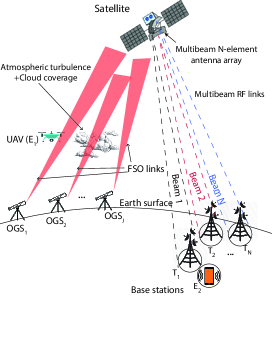
Figure 1: System model.

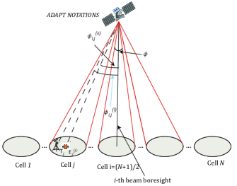
Figure 2: Legitimate and wiretapper nodes’ angles with respect to beams’ boresights.

II-A $S$-$R$ Link

II-A1 Legitimate Link

An OGS with a LOS unblocked by clouds is considered for data transmission. Without loss of generality, all users’ signals are assumed to have the same power.

The received beam at the satellite contains $N$ multiplexed signals transmitted from the transmit gateway. Hence, the received electrical signal vector at the satellite’s $k$-th aperture, after demultiplexing, is expressed as [26]

$$\mathbf{y}_{1}^{(k)}=\sqrt{\omega_{l}P_{S}}\left(\eta I_{k}\right)^{\frac{r}{2}}\mathbf{u}+\mathbf{n}_{k},k=1,\ldots,K,$$ (1)

with $I_{k}=I_{k}^{(a)}I_{k}^{(p)}I_{k}^{(\ell)},$ being the product of the irradiance fluctuation due to atmospheric turbulence, the pointing error due to the beam misalignment, and the free-space path loss, respectively, with $I_{k}^{(\ell)}=I_{t}e^{-\phi d},$ and $I_{t},$ $d$, and $\phi$ denote the laser emittance, the station-satellite distance, and the path loss exponent, respectively. $r\in\{1,2\}$ being a detection-technique dependent parameter, with $r=1$ referring to coherent detection, and $r=2$ stands for direct detection, and $\omega_{l}$ denotes the portion of power received by the satellite’s photodetectors, among the total radiated power from the selected OGS. Also:

• $\mathbf{u}=[u_{1},u_{2},\ldots,u_{N}]^{T}$ denotes the transmitted signal vector of $N$ signals, with the superscript ^T refering to the transpose of a vector. Each unit-power signal is modulated onto one of the $N$ optical sub-carriers, where $\mathbb{E}\left[\mathbf{u}^{H}\mathbf{u}\right]={N},$ with $\mathbb{E}\left[\mathbf{.}\right]$ denoting the expectation operator.

• $P_{S}$ is the OGS transmit power.

• $\mathbf{n}_{k}=[n_{k}^{(1)},n_{k}^{(2)},\ldots,n_{k}^{(N)}]^{T}$ stands for the additive white Gaussian noise (AWGN) process at the satellite with zero mean and the same variance $\sigma_{1}^{2}.$

The satellite converts the received optical waves at the $K$ apertures into electrical signals, and then uses SC to choose the branch with highest instantaneous SNR as: $s^{\ast}=\underset{1\leq k\leq K}{\arg\max}\gamma_{1}^{(k)},$ with $\gamma_{1}^{(k)}=\frac{P_{S}\omega_{l}\left(\eta I_{k}\right)^{r}}{\sigma_{1}^{2}}$ denoting the instantaneous signal-to-noise ratio (SNR) received at the $k$-th satellite’s aperture. Consequently, the combined SNR at the satellite is: $\gamma_{1}=\underset{1\leq k\leq K}{\max}\gamma_{1}^{(k)}.$ Afterwards, the satellite performs a decoding process on the combined electrical signal to regenerate the information signal again.

II-A2 Wiretap Link

The hybrid ground-satellite communication is performed under the malicious attempt of eavesdroppers per each one of the two hops to intercept the legitimate message. For the FSO link, we consider the presence of one wiretapper $e^{(1)}$ located at some altitude within the divergence region of the OGS beam, being able to capture a portion $\omega_{e}=1-\omega_{l}$ of the optical power. That is, the received SNR at $e^{(1)}$ is $\gamma_{1}^{(e)}=\frac{\omega_{e}P_{S}\left(\eta I_{e^{(1)}}\right)^{r}}{\sigma_{e^{(1)}}^{2}},$ with $I_{e^{(1)}}$ and $\sigma_{e^{(1)}}^{2}$ denote the respective optical channel gain, and the variance of the AWGN at $e^{(1)}$, respectively.

In terrestrial FSO communication, the altitude-dependent refractive index structure parameter $C_{n,\varpi}^{2}(h)$ $\left(\varpi\in\{1,e\}\right)$ as well as the Rytov variance $\sigma_{R,\varpi}^{2}$ are two crucial parameters that represent the atmospheric turbulence and pointing error loss impairments. Such parameters are expressed in key system and environment quantities. In the context of vertical optical links in HTS systems, the altitude-dependent refractive structure index parameter in m${}^{-\frac{2}{3}}$ and the Rytov variance can be expressed for the uplink using the Hufnagel-Valley Boundary model as given in [27, Eqs. (4, 9-10)], in terms of the altitude $h$ in meters, the wind speed $V_{w}$ in m/s, the satellite and OGS  altitudes $d_{\varpi}$ and $h_{0}$, the satellite’s zenith angle with respect to the OGS, and the operating wavelength $\lambda.$

Interestingly, $\xi_{\varpi}^{2}=\frac{W_{eq}}{2\sigma_{s}^{2}}$ denotes the pointing error strength, which is the ratio between the equivalent beam waist at the satellite altitude and the beam wander displacement variance, where the last-mentioned quantities are defined in [28], [29, Eq. (2)], and [30, Eq. (8)].

II-B $R$-$D$ Link

The satellite generates $N$ adjacent beams. The received signal vector at the $N$ legitimate end-users and wiretap nodes can be formulated as

$$\mathbf{y}_{2}^{(\varkappa)}=\mathbf{H}^{(\varkappa)}\mathbf{x}+\mathbf{n}_{\varkappa},$$ (2)

with $\varkappa$ equals either $l$ for the legitimate earth stations or $e^{(2)}$ for the second hop’s wiretappers, $P_{SAT}$ is the satellite transmit power, $\mathbf{H}^{(\varkappa)}$ is the channel matrix between the $N$ satellite antennas and the nodes $\left[\varkappa_{i}\right]_{i=1,..,N}$, and $\mathbf{n}_{\varkappa}=\left[n_{\varkappa}^{(i)}\right]_{i=1,..,N}$ is the AWGN vector whose elements are zero mean and with the same variance $\sigma_{\varkappa}^{2}.$

It is known that the channel matrix $\mathbf{H}^{(\varkappa)}$ can be decomposed as [2]

$$\mathbf{H}^{(\varkappa)}=\mathbf{D}^{(\varkappa)}\mathbf{V}^{(\varkappa)},$$ (3)

with $\mathbf{D}^{(\varkappa)}$ being a diagonal matrix containing real-valued random fading coefficients, and $\mathbf{V}^{(\varkappa)}$ entries are path-loss and radiation pattern coefficients, defined by $V_{i,j}^{(\varkappa)}=\frac{c\sqrt{G_{T}^{(j)}G_{R}^{{(\varkappa}_{i}{)}}a_{j}^{(\varkappa_{i})}}}{4\pi fr^{(\varkappa_{i})}\sqrt{\kappa TB_{W}}}$[2], where $c$ being the light celerity in the free space, $G_{T}^{(j)}$ and $G_{R}^{(\varkappa_{i})}$ are the respective gains of the satellite’s $j$-th transmit antenna and the receive antenna of the node $\varkappa_{i}$, $\kappa$ is the Boltzmann constant, $T$ is the receiver noise temperature, $f$ is the operating frequency, $r^{(\varkappa_{i})}$ is the distance between the satellite and the node $\varkappa_{i}$, and $a_{j}^{(\varkappa_{i})}$ is the normalized beam radiation gain, which can be approximated as $a_{j}^{(\varkappa_{i})}\approx\left(\frac{J_{1}\left(\vartheta_{j}^{(\varkappa_{i})}\right)}{2\vartheta_{j}^{(\varkappa_{i})}}+36\frac{J_{3}\left(\vartheta_{j}^{(\varkappa_{i})}\right)}{\left(\vartheta_{j}^{(\varkappa_{i})}\right)^{3}}\right)^{2}$ [17], with $\vartheta_{j}^{(x_{i})}=2.07123\frac{\sin\left(\phi_{j}^{(\varkappa_{i})}\right)}{\phi_{j,3\text{dB}}},$ and $J_{n}(.)$ denotes the $n$-th order Bessel function of the first kind [31, Eq. (8.402)], and $\phi_{j}^{(\varkappa_{i})}$ denote the angle between the node $\varkappa_{i}$ and the $j$-th beam boresight as indicated in (2), given as

$$\phi_{j}^{(\varkappa_{i})}=\left\{\begin{array}[]{c}\phi\left(i-j\right)+\phi_{j}^{(\varkappa_{j})},\text{ }j\geq i\\ \phi\left(i-j\right)-\phi_{j}^{(\varkappa_{j})},\text{ }j<i\end{array}\right.,$$ (4)

with $\phi=$ $\frac{\mathcal{D}}{r}$ referring to the beam width angle, with $\mathcal{D}$ being the cells’ diameter assumed to be equal for all cells, and $r$ is the distance between each node $\varkappa_{i}$ and the satellite, assumed to be equal for all nodes (i.e., $r^{(\varkappa_{i})}\approx r,\forall i\leq N)$. Also, $\phi_{j,3\text{dB}}$ denotes the angle corresponding to 3dB power loss of the $j$-th beam.

II-B1 With ZF Precoding

Legitimate Link

We consider the case of a ZF receiver employed in [2], where the transmit signals are precoded, after decoding, at the satellite before transmitting them to the end-users. Thus, the transmit vector $\mathbf{x}$ is expressed as: $\mathbf{x}=\mathbf{Mu},$ where $\mathbf{M=}\sqrt{\varphi}\mathbf{A}$ is a $N\times N$ precoding matrix with $\mathbf{A}\mathcal{=}\left(\mathbf{V}^{(l)}\right)^{-1},$ and

$$\varphi=\frac{P_{SAT}}{N\operatorname{Tr}\left[\left(\mathbf{V}^{(l)}\left(\mathbf{V}^{(l)}\right)^{H}\right)^{-1}\right]},$$ (5)

where the superscript ^H refers to the Hermitian operator defined as the conjugate of the transpose matrix, and $\operatorname{Tr}[.]$ stands for the matrix’s trace.

After performing ZF precoding at the satellite, the received signal and SNR at the $i$-th earth-station, without considering the first hop, can be formulated as follows

$$y_{ZF}^{(l_{i})} = \sqrt{\varphi}D_{i}^{(l)}u_{i}+n^{(l_{i})},$$ (6)

$$\gamma_{ZF}^{(l_{i})} = \overline{\gamma}_{ZF}^{(l_{i})}\left|D_{i}^{(l)}\right|^{2},$$ (7)

with $D_{i}^{(\varkappa)}$ denoting the $i$-th element of the diagonal of $\mathbf{D}^{(\varkappa)},$ and $\overline{\gamma}_{ZF}^{(l_{i})}=\frac{\varphi}{\sigma_{l}^{2}}.$ Since the satellite performs DF protocol, the equivalent received SNR at the $i$-th earth-station is given as

$$\gamma_{eq,ZF}^{(l_{i})}=\min\left(\gamma_{1},\gamma_{ZF}^{(l_{i})}\right).$$ (8)

Wiretap Link

As far as the second hop is concerned, the satellite-stations links are ensured under the potential presence of one  eavesdropper $\left(e_{i}^{(2)}\right)_{1\leq i\leq N}$ per each cell $i$, aiming to intercept the RF beam transmitted to it. The received signal and instantaneous SNR at $e_{i}^{(2)}$ can be expressed, respectively, as follows

$$y_{e_{i}^{(2)},ZF} =\sqrt{\varphi}D_{i}^{\left(e^{(2)}\right)}\sum_{l=1}^{N}u_{l}\sum_{j=1}^{N}V_{i,j}^{\left(e^{(2)}\right)}A_{j,l}+n^{(e_{i}^{(2)})},$$ (9)

$$\gamma_{e_{i}^{(2)},ZF} =\frac{\psi_{i}\gamma_{ZF}^{\left(e_{i}^{(2)}\right)}}{\theta_{i}\gamma_{ZF}^{\left(e_{i}^{(2)}\right)}+1},$$ (10)

where $n^{(e_{i}^{(2)})}$ denotes an AWGN process at $e_{i}^{(2)}$ with zero mean and the same variance for all wiretap nodes $\sigma_{e^{(2)}}^{2},$ $\gamma_{ZF}^{\left(e_{i}^{(2)}\right)}=\overline{\gamma}_{ZF}^{(e_{i})}\left|D_{i}^{\left(e^{(2)}\right)}\right|^{2},$ $\overline{\gamma}_{ZF}^{\left(e_{i}^{(2)}\right)}=$ $\frac{\varphi}{\sigma_{e^{(2)}}^{2}},$ $\psi_{i}=\left(\sum\limits_{j=1}^{N}V_{i,j}^{(e^{(2)})}A_{j,i}\right)^{2},$ and $\theta_{i}=\left(\sum\limits_{m=1,m\neq i}^{N}\sum\limits_{j=1}^{N}V_{i,j}^{(e^{(2)})}A_{j,m}\right)^{2}.$

II-B2 Without ZF Precoding

When no ZF precoding is performed at the transmit OGS, the received signal and SNR at the legitimate earth station $l_{i}$ as well as the eavesdropper $e_{i}^{(2)}$ are given as

$$y_{NZF}^{(\varkappa_{i})} = \sqrt{\frac{P_{SAT}}{N}}D_{i}^{(\varkappa)}\sum_{j=1}^{N}V_{i,j}^{(\varkappa)}u_{j}+n^{(\varkappa_{i})},$$ (11)

$$\gamma_{\varkappa_{i},NZF} = \frac{\Psi^{(\varkappa_{i})}\gamma_{NZF}^{(\varkappa_{i})}}{\Theta^{(\varkappa_{i})}\gamma_{NZF}^{(\varkappa_{i})}+1},$$ (12)

with $\gamma_{NZF}^{(\varkappa_{i})}=\overline{\gamma}_{NZF}^{(\varkappa_{i})}\left|D_{i}^{(\varkappa)}\right|^{2},\overline{\gamma}_{NZF}^{(\varkappa_{i})}=\frac{P_{SAT}}{N\sigma_{\varkappa}^{2}},$ $\Psi^{(\varkappa_{i})}=\left(V_{i,i}^{(\varkappa)}\right)^{2},$ and $\Theta^{(\varkappa_{i})}=\left(\sum\limits_{j=1,j\neq i}^{N}V_{i,j}^{(\varkappa)}\right)^{2}$.

III Statistical properties

In this section, the cumulative distribution function (CDF) of the SNR of the legitimate link both hops, as well as the wiretap link, is expressed in terms of the system and channel parameters.

III-A $S$-$R$ Link

The Gamma-Gamma distribution is considered for modeling the atmospheric turbulence induced-fading with pointing error for each received optical beam. The respective probability density function (PDF) and CDF of the SNRs $\gamma_{1}^{(k)}$ and $\gamma_{1}^{(e)},$ received respectively at the satellite’s $k$-th aperture and the received one at $E_{1},$ are given as [7]

$$f_{\gamma_{1}^{(\varpi)}}(z) =\frac{\mathcal{P}_{\varpi}}{rz}G_{1,3}^{3,0}\left(\Upsilon_{\varpi}\left(\frac{z}{\mu_{r}^{(\varpi)}}\right)^{\frac{1}{r}}\left|\begin{array}[]{c}-;\xi_{\varpi}^{2}+1\\ \xi_{\varpi}^{2},\alpha_{\varpi},\beta_{\varpi};-\end{array}\right.\right),$$ (15)

$$F_{\gamma_{1}^{(\varpi)}}(z) =\frac{\left(2\pi\right)^{1-r}\mathcal{P}_{\varpi}}{r^{2-\alpha_{\varpi}-\beta_{\varpi}}}G_{r+1,3r+1}^{3r,1}\left(\frac{\Upsilon_{\varpi}^{r}z}{r^{2r}\mu_{r}^{(\varpi)}}\left|\begin{array}[]{c}1;\kappa_{1}^{(\varpi)}\\ \kappa_{2}^{(\varpi)};0\end{array}\right.\right),$$ (18)

respectively, with $\Upsilon_{\varpi}=\frac{\xi_{\varpi}^{2}\alpha_{\varpi}\beta_{\varpi}}{\xi_{\varpi}^{2}+1},\varpi\in\{k,e\},$ $\mathcal{P}_{\varpi}=\frac{\xi_{\varpi}^{2}}{\Gamma\left(\alpha_{\varpi}\right)\Gamma\left(\beta_{\varpi}\right)},$ $\mu_{r}^{(\varpi)}=\mathbb{E}\left[\gamma_{1}^{(\varpi)}\right]$, $\kappa_{1}^{(\varpi)}=\left(\frac{\xi_{\varpi}^{2}+i}{r}\right)_{i=1,..,r},$ $\kappa_{2}^{(\varpi)}=\left(\frac{\xi_{\varpi}^{2}+i}{r},\frac{\alpha_{\varpi}+i}{r},\frac{\beta_{\varpi}+i}{r}\right)_{i=0,..,r-1}$, and $G_{p,q}^{m,n}\left(.\left|.\right.\right)$ refers to the Meijer’s $G$-function [32, Eqs. (1.111), (1.112)]. Moreover, the turbulence-induced fading parameters $\alpha_{\varpi}$ and $\beta_{\mathcal{\ \varpi}}$ are expressed terms of the Rytov variance $\sigma_{R,\varpi}^{2}$ given in [27, Eqs. (4, 9-10)] using [33, Eqs. (9-10)]. Without loss of generality, we consider that the fading amplitudes are i.i.d on all branches, that is $\alpha_{k}=\alpha_{1}$, $\beta_{k}=\beta_{1}$, $\mu_{1}^{(k)}=\mu_{1},$ $\xi_{k}=\xi_{1}$ for $k=1,..,K.$

Proposition 1.

The CDF of the combined SNR at the satellite can be expressed as follows

$$F_{\gamma_{1}}(z)=\mathcal{P}_{1}^{K}\sum_{h_{1}+h_{2}+h_{3}=K}\sum\limits_{l=0}^{\infty}\frac{\mathcal{F}_{h_{1},h_{2},h_{3},l}}{\left(\Upsilon z\right)^{-\varrho_{l,h_{1},h_{2},h_{3}}}},$$ (19)

with $\mathcal{F}_{h_{1},h_{2},h_{3},l}=\frac{K!}{h_{1}!h_{2}!h_{3}!}\left(a_{0}^{(1)}\right)^{h_{1}}\sum\limits_{q_{2}+q_{3}=l}c_{q_{2}}^{(2)}c_{q_{3}}^{(3)},$ $a_{0}^{(1)}=\frac{\Gamma\left(\alpha_{1}-\xi_{1}^{2}\right)\Gamma\left(\beta_{1}-\xi_{1}^{2}\right)}{\xi_{1}^{2}}$, $\Upsilon=\frac{\xi_{1}^{2}\alpha_{1}\beta_{1}}{\mu_{1}\left(\xi_{1}^{2}+1\right)},$ $\varrho_{l,h_{1},h_{2},h_{3}}=l+h_{1}\xi_{1}^{2}+h_{2}\alpha_{1}+h_{3}\beta_{1}$,

$$c_{m}^{(i)}=\left\{\begin{array}[]{l}\left(a_{0}^{(i)}\right)^{h_{i}},m=0\\ \frac{1}{ma_{0}}\sum\limits_{j=1}^{m}\left(jh_{i}-m+j\right)a_{j}^{(i)}c_{m-j}^{(i)};m\geq 1\end{array}\right.,$$ (20)

and $a_{l}^{(2)}=\frac{(-1)^{l}\Gamma\left(\beta_{1}-\alpha_{1}-l\right)}{l!\left(\xi_{1}^{2}-\alpha_{1}-l\right)\left(l+\alpha_{1}\right)},a_{l}^{(3)}=\frac{(-1)^{l}\Gamma\left(\alpha_{1}-\beta_{1}-l\right)}{l!\left(\xi_{1}^{2}-\beta_{1}-l\right)\left(l+\beta_{1}\right)}.$

Proof:

The proof is provided in Appendix A. ∎

III-B $R$-$D$ Link

III-B1 With ZF Precoding

On the other hand, shadowed-Rician fading channel is considered for the satellite RF links, where the PDF of the SNR $\gamma_{ZF}^{(\varkappa_{i})}$ can be calculated by applying Jacobi transform on the fading envelope PDF given in [34] as follows

$$f_{\gamma_{ZF}^{(\varkappa_{i})}}\left(z\right)=\frac{\lambda_{\varkappa_{i}}}{\overline{\gamma}_{ZF}^{(\varkappa_{i})}}e^{-\frac{\rho_{\varkappa_{i}}z}{\overline{\gamma}_{ZF}^{(\varkappa_{i})}}}\text{ }_{1}F_{1}\left(m_{s}^{(\varkappa_{i})};1;\frac{\delta_{\varkappa_{i}}z}{\overline{\gamma}_{ZF}^{(\varkappa_{i})}}\right),$$ (21)

with$\ {}_{1}F_{1}(.;.;.)$ denoting the confluent hypergeometric function [31, Eq. (9.210)], and
$\lambda_{\varkappa_{i}}=\frac{1}{2b_{\varkappa_{i}}}\left(\frac{2b_{\varkappa_{i}}m_{s}^{(\varkappa_{i})}}{2b_{\varkappa_{i}}m_{s}^{(\varkappa_{i})}+\Omega_{s}^{(\varkappa_{i})}}\right)^{m_{s}^{(\varkappa_{i})}},$ $\rho_{\varkappa_{i}}=\frac{1}{2b_{\varkappa_{i}}},$ $\delta_{\varkappa_{i}}=\frac{\Omega_{s}^{(\varkappa_{i})}}{2b_{\varkappa_{i}}\left(2bm_{s}^{(\varkappa_{i})}+\Omega_{s}^{(\varkappa_{i})}\right)}.$ Also, $\Omega_{s}^{(\varkappa_{i})}$, $2b_{\varkappa_{i}},$ and $m_{s}^{(\varkappa_{i})}$ stand for the average power of LOS and multipath components, and the fading severity parameter, respectively.

Consequently, by representing the hypergeometric function ${}_{1}F_{1}\left(.;.;.\right)$ through the finite series [35, Eq. (9)] for integer parameter values, and using [31, Eq. (3.351.1)], the respective CDF is expressed as

$$F_{\gamma_{ZF}^{(\varkappa_{i})}}\left(z\right)=\lambda_{\varkappa_{i}}\sum\limits_{n=0}^{m_{s}^{(\varkappa_{i})}-1}\binom{m_{s}^{(\varkappa_{i})}-1}{n}\frac{\delta_{\varkappa_{i}}^{n}}{v_{\varkappa_{i}}^{n+1}n!}\gamma_{inc}\left(n+1,\frac{v_{\varkappa_{i}}z}{\overline{\gamma}_{ZF}^{(\varkappa_{i})}}\right),$$ (22)

where $\gamma_{inc}\left(.,.\right)$ stands for the lower incomplete Gamma function [31, Eq. (8.350.1)], with $v_{\varkappa_{i}}=\rho_{\varkappa_{i}}-\delta_{\varkappa_{i}}$. Furthermore, the CDF and PDF of the end-to-end SINR in (10) at $e_{i}^{(2)}$ are expressed as

$$F_{\gamma_{e_{i}^{(2)},ZF}}\left(z\right) =\left\{\begin{array}[]{l}F_{\gamma_{ZF}^{\left(e_{i}^{(2)}\right)}}\left(\frac{z}{\psi_{i}-\theta_{i}z}\right);z<\mathscr{L}_{i}\\ 1;z\geq\mathscr{L}_{i}\end{array}\right.,$$ (25)

$$f_{\gamma_{e_{i}^{(2)},ZF}}\left(z\right) =\left\{\begin{array}[]{l}\frac{\psi_{i}}{\left(\psi_{i}-\theta_{i}z\right)^{2}}\frac{\partial F_{\gamma_{ZF}^{\left(e_{i}^{(2)}\right)}}\left(\frac{z}{\psi_{i}-\theta_{i}z}\right)}{\partial z};z<\mathscr{L}_{i}\\ 0;z\geq\mathscr{L}_{i}\end{array}\right..$$ (28)

with $\mathscr{L}_{i}=\frac{\psi_{i}}{\theta_{i}}$.

III-B2 Without ZF Precoding

Importantly, when no ZF precoding is performed, the CDF of the received SNR at node $\varkappa_{i},$ given in (12), can be expressed as

$$F_{\gamma_{\varkappa_{i},NZF}}\left(z\right)=\Pr\left[\gamma_{NZF}^{(\varkappa_{i})}\left(\Psi^{(\varkappa_{i})}-\Theta^{(\varkappa_{i})}z\right)<z\right],$$ (29)

where two cases are distinguished, namely $z<\mathcal{L}^{(\varkappa_{i})}$ and $z\geq\mathcal{L}^{(\varkappa_{i})},$ with $\mathcal{L}^{(\varkappa_{i})}=\frac{\Psi^{(\varkappa_{i})}}{\Theta^{(\varkappa_{i})}}.$ Similarly to the ZF precoding case, the CDF and PDF of the received SNR at node $\varkappa_{i}$ are given as

$$F_{\gamma_{\varkappa_{i},NZF}}\left(z\right) =\left\{\begin{array}[]{l}F_{\gamma_{NZF}^{(\varkappa_{i})}}\left(\frac{z}{\Psi^{(\varkappa_{i})}-\Theta^{(\varkappa_{i})}z}\right);z<\mathcal{L}^{(\varkappa_{i})}\\ 1;z\geq\mathcal{L}^{(\varkappa_{i})}\end{array}\right.,$$ (32)

$$\text{ }f_{\gamma_{\varkappa_{i},NZF}}\left(z\right) =\left\{\begin{array}[]{l}\frac{\Psi^{(\varkappa_{i})}}{\left(\Psi^{(\varkappa_{i})}-\Theta^{(\varkappa_{i})}z\right)^{2}}\frac{\partial F_{\gamma_{NZF}^{(\varkappa_{i})}}\left(\frac{z}{\Psi^{(\varkappa_{i})}-\Theta^{(\varkappa_{i})}z}\right)}{\partial z};z<\mathcal{L}^{(\varkappa_{i})}\\ 0;z\geq\mathcal{L}^{(\varkappa_{i})}\end{array}\right..$$ (35)

with $F_{\gamma_{NZF}^{(\varkappa_{i})}}\left(.\right)$ is obtained from (22) by replacing $\overline{\gamma}_{ZF}^{(\varkappa_{i})}$ with $\overline{\gamma}_{NZF}^{(\varkappa_{i})}$.

IV Secrecy performance analysis

The intercept probability metric is defined as the probability that the secrecy capacity, which is the difference between the capacity of the legitimate links and that of the wiretap channels (i.e., $\{S$-$R,$ $S$-$e^{(1)}\},$ $\{R$-$l_{i},$ $R$-$e_{i}^{(2)}\})$, equals to zero. Additionally, from [36, Eq. (26)] and [37], the respective channel capacities of the FSO legitimate and wiretap links are given for coherent detection techniques as

$$C_{\varrho}=\log_{2}\left(1+Y_{\varrho}\right),$$ (36)

with $\left(\varrho,Y_{\varrho}\right)$ equals either $\left(1,\gamma_{1}\right)$ or $\left(e^{(1)},\gamma_{1}^{(e)}\right).$

On the other hand, the system’s intercept probability is defined as

$$P_{int,\Xi}^{(i)} =\Pr\left(C_{s,\Xi}^{(i)}=0\right)$$

$$=\Pr\left(\left.C_{s,\Xi}^{(i)}=0\right|\gamma_{1}>\gamma_{th}\right)\Pr\left(\gamma_{1}>\gamma_{th}\right)$$

$$+\Pr\left(\left.C_{s,\Xi}^{(i)}=0\right|\gamma_{1}<\gamma_{th}\right)\Pr\left(\gamma_{1}<\gamma_{th}\right),$$ (37)

where $\gamma_{th}$ is a decoding threshold SNR, below which the decoding process fails, $\Xi$ ${\in\{}$ $ZF,NZF\},$ and

$$C_{s,\Xi}^{(i)}=\min\left(C_{s}^{(1)},C_{s,eq,\Xi}^{(2,i)}\right),$$ (38)

with

$$C_{s}^{(1)}=\log_{2}\left(\frac{1+\gamma_{1}}{1+\gamma_{1}^{(e)}}\right),$$ (39)

and

$$C_{s,eq,\Xi}^{(2,i)}=\min\left(C_{s,\Xi}^{(1,2,i)},C_{s,\Xi}^{(2,i)}\right),$$ (40)

stand for the end-to-end, first hop, and second hops’ secrecy capacities, respectively, considering DF relaying protocol, with

$$C_{s,\Xi}^{(1,2,i)} = \log_{2}\left(\frac{1+\gamma_{1}}{1+\gamma_{e_{i}^{(2)},\Xi}}\right),$$ (41)

$$C_{s,\Xi}^{(2,i)} = \log_{2}\left(\frac{1+\gamma_{l_{i},\Xi}}{1+\gamma_{e_{i}^{(2)},\Xi}}\right).$$ (42)

Therefore, the overall secrecy capacity in (38) can be expressed as

$$C_{s,\Xi}^{(i)}=\min\left(C_{s}^{(1)},C_{s,\Xi}^{(2,i)},C_{s,\Xi}^{(1,2,i)}\right).$$ (43)

Lemma 1.

The system’s intercept probability for DF relaying scheme is given as

$$P_{int,\Xi}^{(i)}=1-\int_{y=\gamma_{th}}^{\infty}f_{\gamma_{1}}\left(y\right)F_{\gamma_{1}^{(e)}}\left(y\right)\mathcal{J}_{\Xi}(y)dy,$$ (44)

where $\mathcal{J}_{\Xi}(y)=\int_{z=0}^{y}f_{\gamma_{e_{i}^{(2)},\Xi}}\left(z\right)F_{\gamma_{l_{i},\Xi}}^{c}\left(z\right)dz,$ with $F_{.}^{c}\left(.\right)$ accounts for the complementary CDF .

Proof:

The proof is provided in Appendix B. ∎

IV-A Exact Analysis

Lemma 2.

The integral $\mathcal{J}_{\Xi}(y)$ in the expression (44) is given for the ZF and NZF cases as

$$\mathcal{J}_{ZF}(y) =\sum\limits_{n_{1}=0}^{m_{s}^{(l_{i})}-1}\sum\limits_{n_{2}=0}^{m_{s}^{\left(e_{i}^{(2)}\right)}-1}\frac{\mathcal{U}_{i}\left(n_{1},n_{2}\right)}{\exp\left(r_{1}^{\left(e_{i}^{(2)}\right)}\right)}\sum\limits_{k_{1}=0}^{n_{1}}\sum\limits_{j=0}^{\infty}\frac{(-1)^{j}}{j!k_{1}!}$$

$$\times\left(\psi_{i}r_{1}^{(l_{i})}r_{1}^{\left(e_{i}^{(2)}\right)}\right)^{j+k_{1}}\sum\limits_{p=0}^{k_{1}+n_{2}+j}\frac{\binom{k_{1}+n_{2}+j}{p}}{\left(-r_{1}^{\left(e_{i}^{(2)}\right)}\right)^{p-n_{2}}}$$

$$\times\left[\begin{array}[]{c}\theta_{i}r_{1}^{\left(e_{i}^{(2)}\right)}\Gamma\left(p+1-k_{1}-j,r_{1}^{\left(e_{i}^{(2)}\right)}\right)\\ -\Gamma\left(p+1-k_{1}-j,\frac{r_{1}^{\left(e_{i}^{(2)}\right)}\psi_{i}}{\psi_{i}-\theta_{i}y}\right)\end{array}\right],$$ (47)

$$\mathcal{J}_{NZF}(y)=\left\{\begin{array}[]{l}\sum\limits_{n_{1}=0}^{m_{s}^{(l_{i})}-1}\sum\limits_{n_{2}=0}^{m_{s}^{\left(e_{i}^{(2)}\right)}-1}\frac{\mathcal{U}_{i}\left(n_{1},n_{2}\right)}{\exp\left(-\mathcal{G}^{\left(l_{i},e_{i}^{(2)}\right)}\right)}\sum\limits_{j=0}^{\infty}\frac{\left(-1\right)^{j}\left(\mathcal{G}^{\left(e_{i}^{(2)},l_{i}\right)}\right)^{j+n_{2}+1}}{k_{1}!j!}\sum\limits_{p=0}^{n_{2}+k_{1}+j}\frac{\binom{n_{2}+k_{1}+j}{p}}{\left(-\mathcal{G}^{\left(l_{i},e_{i}^{(2)}\right)}\right)^{p-k_{1}-j-n_{2}-1}}\\ \times\left[\begin{array}[]{l}\Gamma\left(p-n_{2}-1-j,\mathcal{G}^{\left(l_{i},e_{i}^{(2)}\right)}\right)\\ -\Gamma\left(p-n_{2}-1-j,\frac{\mathcal{G}^{(l_{i},l_{i})}\mathcal{T}_{i}}{\Theta^{(l_{i})}\left(\Psi^{(l_{i})}-\Theta^{(l_{i})}y\right)}+\frac{\mathcal{G}^{\left(l_{i},e_{i}^{(2)}\right)}\Theta^{\left(e_{i}^{(2)}\right)}}{\Theta^{(l_{i})}}\right)\end{array}\right],\mathcal{L}^{(l_{i})}<\mathcal{L}^{\left(e_{i}^{(2)}\right)}\\ \sum\limits_{n_{1}=0}^{m_{s}^{(l_{i})}-1}\sum\limits_{n_{2}=0}^{m_{s}^{\left(e_{i}^{(2)}\right)}-1}\frac{\mathcal{U}_{i}\left(n_{1},n_{2}\right)}{\exp\left(\mathcal{G}^{\left(e_{i}^{(2)},l_{i}\right)}\right)}\sum\limits_{k_{1}=0}^{n_{1}}\sum\limits_{j=0}^{\infty}\frac{(-1)^{k_{1}}\left(\mathcal{G}^{\left(l_{i},e_{i}^{(2)}\right)}\right)^{j+k_{1}}}{k_{1}!j!}\sum\limits_{p=0}^{n_{2}+k_{1}+j}\frac{\binom{n_{2}+k_{1}+j}{p}}{\left(\mathcal{G}^{\left(e_{i}^{(2)},l_{i}\right)}\right)^{p-n_{2}-j-k_{1}}}\\ \times\left[\begin{array}[]{l}\Gamma\left(p-k_{1}-j+1,-\mathcal{G}^{\left(e_{i}^{(2)},l_{i}\right)}\right)\\ -\Gamma\left(p-k_{1}-j+1,\left(\frac{\mathcal{T}_{i}}{\Psi^{\left(e_{i}^{(2)}\right)}-\Theta^{\left(e_{i}^{(2)}\right)}y}-\Theta^{(l_{i})}\right)\frac{\mathcal{G}^{\left(e_{i}^{(2)},e_{i}^{(2)}\right)}}{\Theta^{\left(e_{i}^{(2)}\right)}}\right)\end{array}\right],\mathcal{L}^{(l_{i})}>\mathcal{L}^{\left(e_{i}^{(2)}\right)}\end{array}\right.$$ (32)

and in (32) at the top of the next page  for $y<s_{i}$, with $s_{i}$ equals $\mathscr{L}_{i}$ or $\mathcal{L}^{\left(e_{i}^{(2)}\right)}$ for the ZF and NZF cases, respectively, $r_{1}^{(\varkappa_{i})}=\frac{v_{\varkappa_{i}}}{\overline{\gamma}_{2,ZF}^{(\varkappa_{i})}\theta_{i}},$ $\mathcal{G}^{(a_{i},b_{i})}=\frac{v_{a_{i}}\Psi_{i}^{(b)}}{\mathcal{T}_{i}\overline{\gamma}_{2,NZF}^{(a_{i})}},\left(a,b\in\{l,e^{(2)}\}\right),$ $\mathcal{T}_{i}=\Psi^{\left(e_{i}^{(2)}\right)}\Theta^{(l_{i})}-\Psi^{(l_{i})}\Theta^{\left(e_{i}^{(2)}\right)},$ $\Gamma\left(.,.\right)$ is the upper-incomplete Gamma function [31, Eq. (8.350.2)], and

$\mathcal{U}_{i}\left(n_{1},n_{2}\right)\mathcal{=}\frac{\lambda_{l_{i}}\lambda_{e_{i}^{(2)}}}{n_{2}!}\left(\begin{array}[]{c}m_{s}^{(l_{i})}-1\\ n_{1}\end{array}\right)\left(\begin{array}[]{c}m_{s}^{\left(e_{i}^{(2)}\right)}-1\\ n_{2}\end{array}\right)\frac{\delta_{l_{i}}^{n_{1}}}{v_{l_{i}}^{n_{1}+1}}\frac{\delta_{e_{i}^{(2)}}^{n_{2}}}{v_{e_{i}^{(2)}}^{n_{2}+1}}.$

Remark 1.

It is noteworthy that the system’s IP will be computed for the ZF precoding scenario for two cases, namely $\mathscr{L}_{i}<\gamma_{th}$ and $\mathscr{L}_{i}\geq\gamma_{th},$ while for the non-ZF scenario, the IP expression is limited only to the case when $\mathcal{L}^{\left(e_{i}^{(2)}\right)}<\gamma_{th},$ due to the toughness of the encountered mathematical computation.

Proof:

The proof is provided in Appendix C. ∎

Lemma 3.

The integral $K\left(\varphi\right)=\int_{y=\varphi}^{\infty}f_{\gamma_{1}}\left(y\right)F_{\gamma_{1}^{(e)}}dy$ can be expressed as follows

$$K\left(\varphi\right)=1-F_{\gamma_{1}}\left(\varphi\right)F_{\gamma_{1}^{(e)}}\left(\varphi\right)-\mathcal{H}_{1}+\mathcal{H}_{2}\left(\varphi\right),$$ (33)

with

$$\mathcal{H}_{1}=\frac{\xi_{e}^{2}}{\mathcal{P}_{1}^{-K}}\sum_{h_{1}+h_{2}+h_{3}=K}\sum\limits_{l=0}^{\infty}\mathcal{F}_{h_{1},h_{2},h_{3},l}\frac{\left(\alpha_{e}\right)_{\varrho_{l,h_{1},h_{2},h_{3}}}\left(\beta_{e}\right)_{\varrho_{l,h_{1},h_{2},h_{3}}}}{\left(\xi_{e}^{2}+\varrho_{l,h_{1},h_{2},h_{3}}\right)\Upsilon_{e}^{\varrho_{l,h_{1},h_{2},h_{3}}}},$$ (34)

$$\mathcal{H}_{2}\left(\varphi\right) =\mathcal{P}_{1}^{K}\mathcal{P}_{e}\sum_{h_{1}+h_{2}+h_{3}=K}\sum\limits_{l=0}^{\infty}\frac{\varrho_{l,h_{1},h_{2},h_{3}}\mathcal{F}_{h_{1},h_{2},h_{3},l}}{\varphi^{-\varrho_{l,h_{1},h_{2},h_{3}}}}$$

$$\times G_{3,5}^{3,2}\left(\Upsilon_{e}\varphi\left|\begin{array}[]{c}1-\varrho_{l,h_{1},h_{2},h_{3}},1;\xi_{e}^{2}+1\\ \xi_{e}^{2},\alpha_{e},\beta_{e};0,-\varrho_{l,h_{1},h_{2},h_{3}}\end{array}\right.\right),$$ (37)

where $\left(.\right)_{.}$ stands for the Pochhammer symbol [38, Eq. (06.10.02.0001.01)], and $\Upsilon_{e}=\frac{\xi_{e}^{2}\alpha_{e}\beta_{e}}{\mu_{1}^{(e)}\left(\xi_{e}^{2}+1\right)}.$

Proof:

The proof is provided in Appendix D. ∎

Proposition 2.

The system’s IP closed-form expression is given in (36) at the top of the next page, as well as

$$P_{int,ZF}^{(i)}=\left\{\begin{array}[]{l}1-\mathcal{J}_{ZF}\left(\mathscr{L}_{i}\right)\mathcal{K}\left(\gamma_{th}\right);\mathscr{L}_{i}<\gamma_{th}\\ 1-\mathcal{O}_{1}^{(i)}-\mathcal{O}_{2}^{(i)}-\mathcal{J}_{ZF}\left(\mathscr{L}_{i}\right)\mathcal{K}\left(\mathscr{L}_{i}\right);\gamma_{th}\leq\mathscr{L}_{i}<2\gamma_{th}\\ 1-\mathcal{O}_{1}^{(i)}-\mathcal{O}_{3}^{(i)}-\mathcal{J}_{ZF}\left(\mathscr{L}_{i}\right)\mathcal{K}\left(\mathscr{L}_{i}\right);\mathscr{L}_{i}>2\gamma_{th}\end{array}\right.,$$ (36)

$$P_{int,NZF}^{(i)}=1-\mathcal{J}_{NZF}\left(\min\left[\mathcal{L}^{(l_{i})},\mathcal{L}^{\left(e_{i}^{(2)}\right)}\right]\right)\mathcal{K}\left(\gamma_{th}\right),$$ (37)

for $\mathcal{L}^{\left(e_{i}^{(2)}\right)}<\gamma_{th},$ with

$$\mathcal{O}_{1}^{(i)}=\mathcal{J}_{ZF}\left(\mathscr{L}_{i}\right)\left[\mathcal{K}\left(\gamma_{th}\right)-\mathcal{K}\left(\mathscr{L}_{i}\right)\right],$$ (38)

$$\mathcal{O}_{m+1}^{(i)} =\frac{\mathcal{P}_{1}^{K}\mathcal{P}_{e}}{\exp\left(-r_{1}^{\left(e_{i}^{(2)}\right)}\right)}\sum_{h_{1}+h_{2}+h_{3}=K}\sum\limits_{l=0}^{\infty}\mathcal{F}_{h_{1},h_{2},h_{3},l}\varrho_{l,h_{1},h_{2},h_{3}}$$

$$\times\sum\limits_{n_{1}=0}^{m_{s}^{(l_{i})}-1}\sum\limits_{n_{2}=0}^{m_{s}^{\left(e_{i}^{(2)}\right)}-1}\mathcal{U}_{i}\left(n_{1},n_{2}\right)\sum_{k_{1}=0}^{n_{1}}\sum\limits_{j=0}^{\infty}\frac{\left(r_{1}^{(l_{i})}\psi_{i}\right)^{j+k_{1}}}{j!k_{1}!}$$

$$\times\sum\limits_{p=0}^{k_{1}+n_{2}+j}\frac{\binom{k_{1}+n_{2}+j}{p}\left[\mathcal{B}_{1}^{(m,i)}\mathcal{+B}_{\alpha_{e}}^{(m,i)}\mathcal{+B}_{\beta_{e}}^{(m,i)}\right]}{\left(-r_{1}^{\left(e_{i}^{(2)}\right)}\right)^{p-n_{2}-k_{1}-j}};m=1,2,$$ (39)

and

$$\mathcal{B}_{\xi_{e}^{2}}^{(m,i)} = \left\{\begin{array}[]{l}\mathcal{S}_{i}\left(\xi_{e}^{2},0\right);m=1\\ \mathcal{R}_{i}\left(\xi_{e}^{2},0\right);m=2\end{array}\right.,$$ (42)

$$\mathcal{B}_{x}^{(m,i)} = \left\{\begin{array}[]{l}\sum\limits_{v=0}^{\infty}\mathcal{S}_{i}\left(x,v\right);m=1\\ \sum\limits_{v=0}^{\infty}\mathcal{R}_{i}\left(x,v\right);m=2\end{array}\right.,x\in\left\{\alpha_{e},\beta_{e}\right\},$$ (45)

with $b_{\xi_{e}^{2}}^{(0)}=\frac{\Gamma\left(\alpha_{e}-\xi_{e}^{2}\right)\Gamma\left(\beta_{e}-\xi_{e}^{2}\right)}{\xi_{e}^{2}},$ $b_{\alpha_{e}}^{(v)}=\frac{(-1)^{v}\Gamma\left(\beta_{e}-\alpha_{e}-v\right)}{v!\left(\xi_{e}^{2}-\alpha_{e}-v\right)\left(v+\alpha_{e}\right)},b_{\beta_{e}}^{(v)}=\frac{(-1)^{v}\Gamma\left(\alpha_{e}-\beta_{e}-v\right)}{v!\left(\xi_{e}^{2}-\beta_{e}-v\right)\left(l+\beta_{e}\right)}$,

$\mathcal{C}(x,q,v)=(-1)^{q}\left(g(x,q,v)-1\right)q!,$ $g(x,q,v)=1+q+v+x+\varrho_{l,h_{1},h_{2},h_{3}},$

$$\mathcal{S}_{i}\left(y,v\right) =\frac{\Upsilon_{e}^{y+v}}{\mathscr{L}_{i}^{-\mathcal{C}(y,0,v)}}b_{x}^{(v)}\sum\limits_{q=0}^{\infty}\frac{\left(1-\frac{\mathscr{L}_{i}}{\gamma_{th}}\right)^{q+1}}{q!}$$

$$\times G_{0,3}^{4,0}\left(\left.\frac{r_{1}^{\left(e_{i}^{(2)}\right)}\gamma_{th}}{\mathscr{L}_{i}-\gamma_{th}}\right|\Lambda_{1}\left(y,q,v\right)\right),$$ (46)

$$\mathcal{R}_{i}\left(y,v\right) =\frac{\Upsilon_{e}^{y+v}b_{y}^{(v)}}{\mathscr{L}_{i}^{-\mathcal{C}(y,0,v)}}\sum\limits_{q=0}^{\infty}\frac{\left(\frac{\mathscr{L}_{i}}{\gamma_{th}}-1\right)^{-\mathcal{C}(y,0,v)-q}}{\mathcal{C}(y,q,v)}$$

$$\times G_{0,2}^{3,0}\left(\left.r_{1}^{\left(e_{i}^{(2)}\right)}\right|\Lambda_{2}\left(y,q,v\right)\right)-\frac{\Upsilon_{e}^{y+v}b_{y}^{(v)}\Gamma\left(\mathcal{C}(y,0,v)\right)}{\mathscr{L}_{i}^{-\mathcal{C}(\alpha_{e},0,v)}}$$

$$\times G_{0,1}^{2,0}\left(r_{1}^{\left(e_{i}^{(2)}\right)}\left|\begin{array}[]{c}-;g(y,0,v)\\ 0,-k_{1}-j+p+1;-\end{array}\right.\right),$$ (49)

$\Lambda_{1}\left(x,q,v\right)=\left(\begin{array}[]{c}-;g(x,0,v),1,2+q\\ g(x,q,v),1+q,0,-k_{1}-j+p+1;-\end{array}\right)$, and

$\Lambda_{2}\left(x,q,v\right)=\left(\begin{array}[]{c}-;g(x,0,v),1\\ 0,-k_{1}-j+p+1,g(x,q,v);-\end{array}\right)$

Proof:

The proof is provided in Appendix E. ∎

IV-B Asymptotic Analysis

Proposition 3.

The system’s IP can be asymptotically expanded at high SNR regime (i.e., $\overline{\gamma}_{\Xi}^{(l_{i})},\mu_{1}\rightarrow\infty)$ as follows

$$P_{int,\Xi}^{\left(i,\infty\right)}=G_{c,\Xi}\left(\overline{\gamma}_{\Xi}^{(l_{i})}\right)^{-G_{d}},$$ (50)

with

$$G_{c,\Xi} =\left\{\begin{array}[]{l}\left(a_{0}^{(d)}\mathcal{P}_{1}\left(\epsilon_{\Xi}^{(i)}\Upsilon^{\prime}a^{(\Xi)}\right)^{x_{d}}\right)^{K}F_{\gamma_{1}^{(e)}}\left(a^{(\Xi)}\right)\\ +\mathcal{X}\left(a^{(\Xi)}\right),\text{ if }Kx_{d}<1\text{ }\\ \mathcal{Q}^{(i,\Xi)},\text{ }Kx_{d}>1\end{array}\right.,$$ (54)

$$a^{(\Xi)} =\left\{\begin{array}[]{c}\gamma_{th},\text{ }\Xi=NZF\text{ or }\left(\Xi=ZF\text{ and }\gamma_{th}\geq\mathscr{L}_{i}\right)\\ \mathscr{L}_{i},\text{ }\Xi=ZF\text{ and }\gamma_{th}<\mathscr{L}_{i}\end{array}\right.,$$ (57)

$$G_{d} =\min\left(1,Kx_{d}\right),$$ (58)

where $\Upsilon^{\prime}=\frac{\xi_{1}^{2}\alpha_{1}\beta_{1}}{\xi_{1}^{2}+1},$ $\epsilon_{\Xi}^{(i)}=\frac{\overline{\gamma}_{\Xi}^{(l_{i})}}{\mu_{1}},$ $x_{d}=\underset{i=1,2,3}{\min}\left(x_{i}\right),$ and

$$\mathcal{X}\left(\varphi\right) =\mathcal{P}_{e}\left(a_{0}^{(d)}\mathcal{P}_{1}\left(\epsilon_{\Xi}^{(i)}\Upsilon^{\prime}\right)^{x_{d}}\right)^{K}$$

$$\times\left[\begin{array}[]{l}\frac{\Gamma\left(\alpha_{e}+Kx_{d}\right)\Gamma\left(\beta_{e}+Kx_{d}\right)}{\Upsilon_{e}^{Kx_{d}}\left(\xi_{e}^{2}+Kx_{d}\right)}\\ -\varphi^{Kx_{d}}G_{2,4}^{3,1}\left(\Upsilon_{e}\varphi\left|\begin{array}[]{c}1-Kx_{d};\xi_{e}^{2}+1\\ \xi_{e}^{2},\alpha_{e},\beta_{e};-Kx_{d}\end{array}\right.\right)\end{array}\right].$$ (63)

and $\mathcal{Q}^{(i,ZF)}$, $\mathcal{Q}^{(i,NZF)}$ are given in (48) and (57) at the top of the next page, with $\mathcal{Z}^{(i)}=\frac{v_{l_{i}}\Psi^{\left(e_{i}^{(2)}\right)}}{\mathcal{T}_{i}\exp\left(\mathcal{G}^{\left(e_{i}^{(2)},l_{i}\right)}\right)},$ $E_{i}(.)$ is the exponential integral function [31, Eq. (8.211.1)].

$$Q^{(i,ZF)} =\psi_{i}\exp\left(r_{1}^{\left(e_{i}^{(2)}\right)}\right)\sum\limits_{n_{2}=0}^{m_{s}^{\left(e_{i}^{(2)}\right)}-1}U_{i}\left(0,n_{2}\right)\sum\limits_{p=0}^{n_{2}+1}\binom{n_{2}+1}{p}(-1)^{n_{2}+1-p}\left(r_{1}^{\left(e_{i}^{(2)}\right)}\right)^{n_{2}-p+1}\Gamma\left(p,r_{1}^{\left(e_{i}^{(2)}\right)}\right)$$ (48)

$$\mathcal{Q}^{(i,NZF)}=\left\{\begin{array}[]{l}\mathcal{Z}^{(i)}\sum\limits_{n_{2}=0}^{m_{s}^{\left(e_{i}^{(2)}\right)}-1}\frac{\mathcal{U}_{i}\left(0,n_{2}\right)}{\left(\mathcal{G}^{\left(e_{i}^{(2)},l_{i}\right)}\right)^{-n_{2}-1}}\left(\begin{array}[]{l}E_{i}\left(\mathcal{G}^{\left(e_{i}^{(2)},l_{i}\right)}\right)\\ +\sum\limits_{q=1}^{n_{2}+1}\left(\begin{array}[]{c}n_{2}+1\\ q\end{array}\right)\frac{\gamma_{inc}\left(q,-\mathcal{G}^{\left(e_{i}^{(2)},l_{i}\right)}\right)}{\left(-\Theta^{(l_{i})}\Psi^{\left(e_{i}^{(2)}\right)}\right)^{-q-n_{2}-1}}\end{array}\right),\mathcal{L}^{(l_{i})}<\mathcal{L}^{\left(e_{i}^{(2)}\right)}\\ -\mathcal{Z}^{(i)}\sum\limits_{n_{2}=0}^{m_{s}^{\left(e_{i}^{(2)}\right)}-1}\mathcal{U}_{i}\left(0,n_{2}\right)\left(n_{2}+1\right)!G_{1,2}^{2,0}\left(-\mathcal{G}^{\left(e_{i}^{(2)},l_{i}\right)}\left|\begin{array}[]{c}2+n_{2}\\ 0,1+n_{2}\end{array}\right.\right),\mathcal{L}^{(l_{i})}\geq\mathcal{L}^{\left(e_{i}^{(2)}\right)}\end{array},\right.$$ (57)

Proof:

The proof is provided in Appendix F. ∎

V Numerical results

The derived analytic results, which are validated with their respective Monte Carlo simulations are depicted in this section to analyze the performance of the considered set up. Some illustrative numerical examples are depicted to inspect the effects of the key system parameters on the overall secrecy performance of the considered hybrid terrestrial-satellite link. To this end, the system and channel parameters are set as detailed in Table I. The FSO hop turbulence parameters were computed based on OGS-satellite distance, wavelength, and aperture radius using [27, Eq. (4, 9-10)], [28], [29, Eq. (2)], and [30, Eq. (8)]. Furthermore, the positions of the legitimate and wiretap nodes were set using Table I and based on (4) with  $\phi_{j}^{(l_{j})}=3\times 10^{-3}$ rad, $\phi_{j}^{\left(e_{j}^{(2)}\right)}=6.66\times 10^{-4}$ rad , respectively, except Figs. 7-11, where $\phi_{j}^{\left(e_{j}^{(2)}\right)}=6.66\times 10^{-4}$ rad, $\phi_{j}^{(l_{j})}=5\times 10^{-4}$ rad. Also, the simulation is performed by generating $2\times 10^{6}$ random samples.

TABLE I: Simulation parameters’ values.

Parameter	Value	Parameter	Value	Parameter	Value
$f$	20 GHz	$K$	3 (Except Fig. 4)	$N$	5
$T$	193.15 ${{}^{\circ}}K$	$R_{k}$	50 cm	$r$	6000 km
$B_{w}$	50 MHz	$R_{e}$	100 cm	$V_{w}$	21 m/s
$G_{R}^{\left(l_{i}\right)}$	40 dBi (except Fig. 4)	$\omega_{e}$	0.3 (Except Fig. 6)	$\frac{P_{S}}{\sigma_{1}^{2}}$	$80$ dB (Except Fig. 6)
$G_{R}^{\left(e_{i}^{(2)}\right)}$	25 dBi	$\omega_{l}$	0.7 (Except Fig. 6)	$\frac{P_{S}}{\sigma_{e^{(1)}}^{2}}$	$60$ dB (Except Fig. 6)
$G_{T}^{(i)}$	60 dBi	$m_{s}^{(\varkappa_{i})}$	2	$W_{0}$	8 cm
$\phi_{j,\text{3dB}}$	0.4∘	$\Omega_{s}^{(\varkappa_{i})}$	3 (Except Fig. 6)	$\lambda$	1550 nm
$d_{k}=d_{e}$	6000 Km	$b_{\varkappa_{i}}$	1.4 (Except Fig. 6)	$D$	100 Km
$h_{0}$	25 m	$A$	$1.7\times 10^{-14}$ m${}^{-\frac{2}{3}}$	$\gamma_{th}$	20 dB

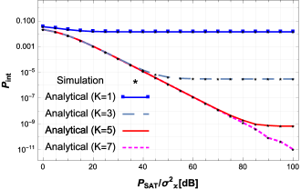
Figure 3: IP versus $\frac{P_{SAT}}{\sigma_{\varkappa}^{2}}$ for various $K$ values.

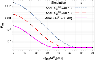
Figure 4: IP versus $\frac{P_{SAT}}{\sigma_{\varkappa}^{2}}$ for various $G_{R}^{(l_{i})}$ values.

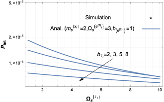
Figure 5: IP without ZF precoding versus $\Omega_{s}^{(l_{i})}$

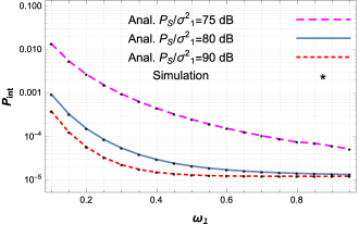
Figure 6: IP with ZF precoding versus $\omega_{l}$ .

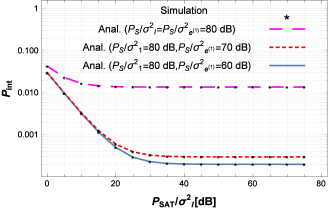
Figure 7: IP with ZF precoding vs $\frac{P_{SAT}}{\sigma_{l}^{2}}.$

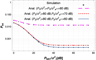
Figure 8: IP without ZF precoding vs $\frac{P_{SAT}}{\sigma_{l}^{2}}$

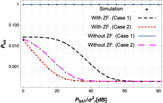
Figure 9: Comparison of the IP of both scenarios: With and without ZF.

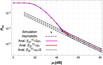
Figure 10: IP with ZF precoding vs $\mu_{1}$.

In Fig. 4, the IP is shown as a function of the average SNR $\frac{P_{SAT}}{\sigma_{\varkappa}^{2}}$ ($\varkappa=\{l,e^{(2)}\}),$ by considering $\frac{P_{SAT}}{\sigma_{l}^{2}}=\frac{P_{SAT}}{\sigma_{e^{(2)}}^{2}},$ for various optical apertures at the satellite. One can ascertain evidently that the secrecy performance decreases as a function of $\frac{P_{SAT}}{\sigma_{\varkappa}^{2}}$, particularly below a certain threshold SNR and for high values of $K$. However, the secrecy gets steady for higher average SNR values. Also, the number of optical apertures at the satellite impacts the secrecy level of the system. The greater the number of apertures, the higher is the legitimate link capacity, and consequently, the more secure is the whole link. Nevertheless, one can note also that above $K=7$ apertures, the IP is not improved significantly.

Fig. 4 shows the IP evolution for the ZF case versus $\frac{P_{SAT}}{\sigma_{\varkappa}^{2}}$ for various values of legitimate receiver antenna gains. One can remark that for increasing the antennas gains of the legitimate users can ensure a significant improvement of the received legitimate SNR, and consequently results in better secrecy performance of the system.

Fig. 6 depicts the IP for the non-ZF case as a function of $\Omega_{s}^{(l_{i})}$ for various values $b_{l_{i}}$, with $\Omega_{s}^{\left(e_{i}^{(2)}\right)}=3,$ $m_{s}^{(x_{i})}=2,$ $b_{e_{i}^{(2)}}=1$, and $\frac{P_{SAT}}{\sigma_{l}^{2}}=\frac{P_{SAT}}{\sigma_{e^{(2)}}^{2}}=40$ dB. One can ascertain that the higher the power of the legitimate link LOS and multipath components $\Omega_{s}^{(l_{i})}$ and $b_{l_{i}},$ the higher the second hop’s legitimate link SNR, which results in a greater overall secrecy capacity. Thus, the system’s secrecy gets better.

Fig. 6 shows the IP evolution versus the power portion received at the satellite $\omega_{l},$ for a fixed transmit power-to-noise ratio of the second hop $\frac{P_{SAT}}{\sigma_{l}^{2}}=\frac{P_{SAT}}{\sigma_{e^{(2)}}^{2}}=40$ dB, and $\frac{P_{S}}{\sigma_{1}^{2}}=50,$ $60$, and $70$ dB with $\frac{P_{S}}{\sigma_{1}^{2}}=\frac{P_{S}}{\sigma_{e^{(1)}}^{2}}+20$ dB. One can notice that the system’s secrecy improves by increasing the portion of power received by the legitimate node (i.e., the satellite). In fact, as $\omega_{l}$ is increasing, the SNR of the first hop’s legitimate link as well as the equivalent end-to-end SNR increase. As a result, the overall secrecy capacity in (38) gets greater too, which leads to a decrease in the system’s IP. Nevertheless, at higher $\omega_{l}$ values (higher $\gamma_{1}$), the IP gets steady at a certain level. In fact, from (38), the overall secrecy capacity will be restricted to the minimum of the two hops’ secrecy capacities (i.e., $C_{s,eq,\Xi}^{(2,i)})$, regardless the increase in $\omega_{l}$ (i.e., $C_{s}^{(1)}$ increase).

Figs. 8 and 8 depict the IP evolution versus $\frac{P_{SAT}}{\sigma_{l}^{2}},$ for the ZF and the non-ZF precoding scenarios, respectively, for three different scenarios of the first hop SNRs, namely $\frac{P_{S}}{\sigma_{1}^{2}}=80$ dB, and $\frac{P_{S}}{\sigma_{e^{(1)}}^{2}}=60,$ $70,$and $80$ dB. One can remarkably note that for the both abovementioned scenarios, the IP is improved with increasing the difference between the FSO legitimate and wiretapper average SNRs. Nevertheless, the greater the gap, the lesser the secrecy improvement.

In Fig. 10, the IP is shown versus $\frac{P_{SAT}}{\sigma_{l}^{2}}$ for two scenarios: (i) ZF precoding case, and (ii) non-ZF precoding. We fixed again $\frac{P_{S}}{\sigma_{1}^{2}}=\frac{P_{S}}{\sigma_{e^{(1)}}^{2}}=30$ dB. Importantly, we depict the IP for the two abovementioned scenarios, as computed in the non-ZF scenario in (37), for case 1 $\left(\mathcal{L}^{(l_{i})}<\mathcal{L}^{\left(e_{i}^{(2)}\right)}\right)$ and case 2 $\left(\mathcal{L}^{(l_{i})}\geq\mathcal{L}^{\left(e_{i}^{(2)}\right)}\right)$, based on Table I and (4) with $\phi_{j}^{\left(e_{j}^{(2)}\right)}=6.66\times 10^{-4}$ rad, $\phi_{j}^{(l_{j})}=5\times 10^{-4}$ rad $\left(\text{i.e., case 1}\right)$ and  $\phi_{j}^{(l_{j})}=3\times 10^{-3}$ rad, $\phi_{j}^{\left(e_{j}^{(2)}\right)}=6.66\times 10^{-4}$ rad $\left(\text{i.e.,}\mathcal{\ }\text{case 2}\right)$, respectively. On the other hand, the two aforementioned cases were implemented for the ZF precoding expression by adopting the same two abovementioned scenarios of $\phi_{j}^{(\varkappa_{i})}$. One can ascertain evidently that the ZF precoding case outperforms its non-ZF counterpart for case 1. Thus, the closer the legitimate node to the beams boresight (cells’ centers) compared to the wiretap node, the worse is the secrecy. Additionally, the non-ZF scenario admits a steady IP behavior at high SNR regime regardless of the increase in $\frac{P_{SAT}}{\sigma_{l}^{2}}.$ In fact, from (12), one can notice clearly that at high $\overline{\gamma}_{NZF}^{(\varkappa_{i})}$ values, the received SNRs$\ \gamma_{\varkappa_{i},NZF}$ reduce to $\mathcal{L}^{(l_{i})}\$and $\mathcal{L}^{\left(e_{i}^{(2)}\right)},$ for $\varkappa=l,e^{(2)},$ respectively. Given that $\mathcal{L}^{(l_{i})}<\mathcal{L}^{\left(e_{i}^{(2)}\right)},$ it follows that the wiretapper received SNR is always greater than the legitimate one for high average SNR values, leading to steady IP performance. On the other hand, the IP shows a distinguished behavior for the second case $\left(\text{i.e., }\phi_{j}^{(l_{i})}\geq\phi_{j}^{\left(e_{i}^{(2)}\right)}\right)$, where the non-ZF case outperforms the ZF precoding one. In fact, and similarly to the previous case, as $\mathcal{L}^{(l_{i})}\geq\mathcal{L}^{\left(e_{i}^{(2)}\right)}$, the legitimate SNR is most likely greater than the wiretapper one. Thus, the farther the legitimate node from the cells’ center compared to $e_{i}^{(2)},$ the better the secrecy performance. Additionally, due to ZF SNR normalization in (5) and (7), the ZF precoding average SNR most likely drops below $\mathcal{L}^{(l_{i})}$, resulting in secrecy performance degradation.

Fig. 10 represents the IP evolution versus $\mu_{1}$, when ZF precoding is performed, for various SNR  proportionality values $\left(\text{i.e., }\mu_{1}=\epsilon_{i}\overline{\gamma}_{ZF}^{\left(l_{i}\right)},\text{ }\epsilon_{i}=\frac{1}{2},1,2\right)$, and for eavesdropper average SNR value $\frac{P_{S}}{\sigma_{e^{(1)}}^{2}}=\frac{P_{S}}{\sigma_{e^{(2)}}^{2}}=30$ dB. We can ascertain that the higher the first hop average SNR (i.e., higher OGS transmit power or lower satellite reception noise), the better the overall system’s secrecy. Furthermore, the asymptotic curves match tightly the exact ones, which proves the accuracy of the retrieved expressions in high SNR regime.

VI Conclusion

The secrecy performance of a hybrid terrestrial-satellite communication system, operating with an optical feeder in the presence of potential wiretappers in both hops is assessed. Statistical properties of the per-hop SNR of the legitimate, as well as the wiretap link, are derived. Furthermore, a novel expression for the IP for a dual-hop DF-based communication system is retrieved, based on which the analyzed system’s IP metric is investigated in closed-form and asymptotic expressions in terms of key system and channel parameters for several parameters’ values cases. The analysis was performed for two scenarios, namely by considering ZF precoding at the satellite, and by assuming direct satellite delivery to the earth-stations (i.e., non-ZF). The obtained analytical results show that the system’s secrecy can be significantly improved by increasing the number of optical photodetectors at the satellite, gateway and satellite transmit powers, as well as antennas gains. Furthermore, ZF precoding technique improves the system’s secrecy level compared to the non-ZF case for some specific nodes’ positions scenarios.

A potential extension of this work might be the consideration of amplify-and-forward (AF) relaying scheme as well as investigating the impact of cloud coverage on the overall secrecy performance.

Appendix A: Proof of Proposition 1

The SNR $\gamma_{1}$ is the maximum among individual SNRs $\gamma_{1}^{(k)}$ at each of the $K$ photodetectors at the satellite. Consequently, its respective CDF can be expressed in the case of i.i.d fading amplitudes, using (18) for coherent detection (i.e., $r=1$) as

$$F_{\gamma_{1}}(z)=\left[\mathcal{P}_{1}G_{2,4}^{3,1}\left(\Upsilon z\left|\begin{array}[]{c}1;\xi_{1}^{2}+1\\ \xi_{1}^{2},\alpha_{1},\beta_{1};0\end{array}\right.\right)\right]^{K},$$ (58)

with $\Upsilon$ is defined in Proposition 1. By making use of the residues theorem [39, Theorem 1.2] on the Meijer’s $G$-function above, one obtains

$$F_{\gamma_{1}}(z)=\mathcal{P}_{1}^{K}\left[\Delta_{1}+\Delta_{2}+\Delta_{3}\right]^{K},$$ (59)

with

$$\Delta_{i}=\left(\Upsilon z\right)^{x_{i}}\text{ }\mathcal{E}_{i},$$ (60)

and $\mathcal{E}_{i}=\sum_{l=0}^{\infty}a_{l}^{(i)}\left(\Upsilon z\right)^{l},$ and $x_{i}\in\{\xi_{1}^{2},\alpha_{1},\beta_{1}\}.$

Using the multinomial theorem, the CDF can be formulated as

$$F_{\gamma_{1}}(z)=\mathcal{P}_{1}^{K}\sum_{h_{1}+h_{2}+h_{3}=K}\frac{K!}{h_{1}!h_{2}!h_{3}!}\frac{\left(\Upsilon z\right)^{h_{1}\xi_{1}^{2}+h_{2}\alpha_{1}+h_{3}\beta_{1}}}{\mathcal{E}_{1}^{-h_{1}}\mathcal{E}_{2}^{-h_{2}}\mathcal{E}_{3}^{-h_{3}}}.$$ (61)

Involving the identity [31, Eq. (0.314)], we have the following: $\mathcal{E}_{i}^{h_{i}}=\sum\limits_{l=0}^{\infty}c_{l}^{(i)}z^{l}\Upsilon^{l},$ where the coefficients $c_{l}^{(i)}$ are defined in Proposition 1. Consequently, we have the following

$$\mathcal{E}_{1}^{h_{1}}\mathcal{E}_{2}^{h_{2}}\mathcal{E}_{3}^{h_{3}}=c_{1}^{(1)}\sum\limits_{l=0}^{\infty}\left(\sum\limits_{q_{2}+q_{3}=l}c_{q_{2}}^{(2)}c_{q_{3}}^{(3)}\right)z^{l}\Upsilon^{l}.$$ (62)

By involving (62) into (61), Proposition 1 is attained.

Appendix B: Proof of Lemma 1

Relying on the probability theory, we have the following

$$\Pr\left(C_{s,\Xi}^{(i)}=0,\gamma_{1}>\gamma_{th}\right)=\Pr\left(\gamma_{1}>\gamma_{th}\right)-\Pr\left(C_{s,\Xi}^{(i)}>0,\gamma_{1}>\gamma_{th}\right).$$ (63)

When $\gamma_{1}<\gamma_{th},$ the satellite fails at decoding the information message. Therefore, no signal will be transmitted to the legitimate earth-stations $l_{i}$ as well as the eavesdroppers $e_{i}^{(2)}.$ Hence, we have $\gamma_{l_{i},\Xi}=\gamma_{e_{i}^{(2)},\Xi}=0$, which yields from (42) and (43) that $C_{s,\Xi}^{(i)}=0$ and $\Pr\left(\left.C_{s,\Xi}^{(i)}=0\right|\gamma_{1}<\gamma_{th}\right)=1.$ As a result, by making use of (63) into (37), the overall IP expression reduces to

$$P_{int,\Xi}^{(i)}=1-\Pr\left(C_{s,\Xi}^{(i)}>0,\gamma_{1}>\gamma_{th}\right).$$ (64)

By involving (43) into the above equation and relying on probability theory and some algebraic manipulations, one obtains

$$P_{int,\Xi}^{(i)}=1-\underset{\mathcal{I}}{\underbrace{\Pr\left(\gamma_{1}>\gamma_{1}^{(e)},\gamma_{1}>\gamma_{e_{i}^{(2)},\Xi},\gamma_{l_{i},\Xi}>\gamma_{e_{i}^{(2)},\Xi},\gamma_{1}>\gamma_{th}\right)}}.$$ (65)

The above probability $\mathcal{I}$ can be expressed as $\mathcal{I}=\sum\limits_{i=1}^{6}\mathcal{I}_{i},$ with $I_{i}$ are the probabilities associated with the events $\boldsymbol{E}_{i}$ shown in Table II.

TABLE II: Six possible events for $\mathcal{I}$.

	Event		Event
$\boldsymbol{E}_{1}$	$\gamma_{1}>\gamma_{1}^{(e)}>\gamma_{e_{i}^{(2)},\Xi}>\gamma_{th}$	$\boldsymbol{E}_{4}$	$\gamma_{1}>\gamma_{th}>\gamma_{1}^{(e)}>\gamma_{e_{i}^{(2)},\Xi}$
$\boldsymbol{E}_{2}$	$\gamma_{1}>\gamma_{e_{i}^{(2)},\Xi}>\gamma_{1}^{(e)}>\gamma_{th}$	$\boldsymbol{E}_{5}$	$\gamma_{1}>\gamma_{e_{i}^{(2)},\Xi}>\gamma_{th}>\gamma_{1}^{(e)}$
$\boldsymbol{E}_{3}$	$\gamma_{1}>\gamma_{th}>\gamma_{e_{i}^{(2)},\Xi}>\gamma_{1}^{(e)}$	$\boldsymbol{E}_{6}$	$\gamma_{1}>\gamma_{1}^{(e)}>\gamma_{th}>\gamma_{e_{i}^{(2)},\Xi}$

Relying on Table II, one can see that

$$\mathcal{I}_{1} \mathcal{=}\int_{y=\gamma_{th}}^{\infty}F_{\gamma_{1}}^{c}\left(y\right)f_{\gamma_{1}^{(e)}}\left(y\right)dy\int_{z=\gamma_{th}}^{y}f_{\gamma_{e_{i}^{(2)},\Xi}}\left(z\right)F_{\gamma_{l_{i},\Xi}}^{c}\left(z\right)dz,$$ (66)

$$\mathcal{I}_{2} =\int_{z=\gamma_{th}}^{\infty}F_{\gamma_{1}}^{c}\left(z\right)f_{\gamma_{e_{i}^{(2)},\Xi}}\left(z\right)F_{\gamma_{l_{i},\Xi}}^{c}\left(z\right)\int_{y=\gamma_{th}}^{z}f_{\gamma_{1}^{(e)}}\left(y\right)dydz,$$ (67)

$$\mathcal{I}_{3} =\int_{x=\gamma_{th}}^{\infty}\int_{y=0}^{\gamma_{th}}\int_{z=y}^{\gamma_{th}}\int_{t=z}^{\infty}f_{\gamma_{1}}\left(x\right)f_{\gamma_{1}^{(e)}}\left(y\right)f_{\gamma_{e_{i}^{(2)},\Xi}}\left(z\right)$$ (68)

$$\times f_{\gamma_{l_{i},\Xi}}\left(t\right)dxdydzdt,$$

$$\mathcal{I}_{4} =\int_{x=\gamma_{th}}^{\infty}\int_{z=0}^{\gamma_{th}}\int_{y=z}^{\gamma_{th}}\int_{t=z}^{\infty}f_{\gamma_{1}}\left(x\right)f_{\gamma_{1}^{(e)}}\left(y\right)f_{\gamma_{e_{i}^{(2)},\Xi}}\left(z\right)$$ (69)

$$\times f_{\gamma_{l_{i},\Xi}}\left(t\right)dxdydzdt,$$

$$\mathcal{I}_{5} =\int_{y=0}^{\gamma_{th}}\int_{x=\gamma_{th}}^{\infty}\int_{z=\gamma_{th}}^{x}\int_{t=z}^{\infty}f_{\gamma_{1}}\left(x\right)f_{\gamma_{1}^{(e)}}\left(y\right)f_{\gamma_{e_{i}^{(2)},\Xi}}\left(z\right)$$ (70)

$$\times f_{\gamma_{2,\Xi}^{(l_{i})}}\left(t\right)dxdydzdt,$$

$$\mathcal{I}_{6} \mathcal{=}\int_{x=\gamma_{th}}^{\infty}\int_{y=\gamma_{th}}^{x}\int_{z=0}^{\gamma_{th}}\int_{t=z}^{\infty}f_{\gamma_{1}}\left(x\right)f_{\gamma_{1}^{(e)}}\left(y\right)f_{\gamma_{e_{i}^{(2)},\Xi}}\left(z\right)$$

$$\times f_{\gamma_{l_{i},\Xi}}\left(t\right)dxdydzdt.$$ (71)

By applying an integration by parts on (66) and (68) with $u^{\prime}(y)=f_{\gamma_{1}^{(e)}}\left(y\right),$ and on (70) with $u^{\prime}(x)=f_{\gamma_{1}}\left(x\right)$ alongside with some algebraic manipulations, one obtains

$$\mathcal{I}_{1} =\int_{y=\gamma_{th}}^{\infty}f_{\gamma_{1}}\left(y\right)F_{\gamma_{1}^{(e)}}\left(y\right)dy\int_{z=\gamma_{th}}^{y}f_{\gamma_{e_{i}^{(2)},\Xi}}\left(z\right)F_{\gamma_{l_{i},\Xi}}^{c}\left(z\right)dz$$

$$-\int_{y=\gamma_{th}}^{\infty}F_{\gamma_{1}}^{c}\left(y\right)f_{\gamma_{e_{i}^{(2)},\Xi}}\left(y\right)F_{\gamma_{l_{i},\Xi}}^{c}\left(y\right)F_{\gamma_{1}^{(e)}}\left(y\right)dy.$$ (72)

$$\mathcal{I}_{3}=F_{\gamma_{1}}^{c}\left(\gamma_{th}\right)\int_{y=0}^{\gamma_{th}}F_{\gamma_{1}^{(e)}}\left(y\right)f_{\gamma_{e_{i}^{(2)},\Xi}}\left(y\right)F_{\gamma_{l_{i},\Xi}}^{c}\left(y\right)dy.$$ (73)

$$\mathcal{I}_{5}=F_{\gamma_{1}^{(e)}}\left(\gamma_{th}\right)\left\{\begin{array}[]{c}\int_{z=\gamma_{th}}^{\infty}f_{\gamma_{e_{i}^{(2)},\Xi}}\left(z\right)F_{\gamma_{2}}^{c}\left(z\right)dz\\ -\int_{x=\gamma_{th}}^{\infty}F_{\gamma_{1}}\left(x\right)f_{\gamma_{e_{i}^{(2)},\Xi}}\left(x\right)F_{\gamma_{2}}^{c}\left(x\right)dx\end{array}\right\}$$ (74)

Additionally, by using the basic definition of the CDF in terms of the respective PDF, it yields

$$\mathcal{I}_{2} =\int_{z=\gamma_{th}}^{\infty}F_{\gamma_{1}}^{c}\left(z\right)f_{\gamma_{e_{i}^{(2)},\Xi}}\left(z\right)F_{\gamma_{l_{i},\Xi}}^{c}\left(z\right)F_{\gamma_{1}^{(e)}}\left(z\right)dz$$

$$-F_{\gamma_{1}^{(e)}}\left(\gamma_{th}\right)\int_{z=\gamma_{th}}^{\infty}F_{\gamma_{1}}^{c}\left(z\right)f_{\gamma_{e_{i}^{(2)},\Xi}}\left(z\right)F_{\gamma_{l_{i},\Xi}}^{c}\left(z\right)dz.$$ (75)

$$\mathcal{I}_{4} =F_{\gamma_{1}}^{c}\left(\gamma_{th}\right)F_{\gamma_{1}^{(e)}}\left(\gamma_{th}\right)\int_{z=0}^{\gamma_{th}}f_{\gamma_{e_{i}^{(2)},\Xi}}\left(z\right)F_{\gamma_{l_{i},\Xi}}^{c}\left(z\right)dz$$

$$-F_{\gamma_{1}}^{c}\left(\gamma_{th}\right)\int_{z=0}^{\gamma_{th}}f_{\gamma_{e_{i}^{(2)},\Xi}}\left(z\right)F_{\gamma_{l_{i},\Xi}}^{c}\left(z\right)F_{\gamma_{1}^{(e)}}\left(z\right)dz.$$ (76)

$$\mathcal{I}_{6} =\left[\int_{x=\gamma_{th}}^{\infty}f_{\gamma_{1}}\left(x\right)F_{\gamma_{1}^{(e)}}\left(x\right)dx\right]\int_{z=0}^{\gamma_{th}}f_{\gamma_{e_{i}^{(2)},\Xi}}\left(z\right)F_{\gamma_{l_{i},\Xi}}^{c}\left(z\right)dz$$

$$-F_{\gamma_{1}}^{c}\left(\gamma_{th}\right)F_{\gamma_{1}^{(e)}}\left(\gamma_{th}\right)\int_{z=0}^{\gamma_{th}}f_{\gamma_{e_{i}^{(2)},\Xi}}\left(z\right)F_{\gamma_{l_{i},\Xi}}^{c}\left(z\right)dz.$$ (77)

By summing the terms $\mathcal{I}_{3},$ $\mathcal{I}_{4},$ and $\mathcal{I}_{6},$ one obtains

$$\mathcal{I}_{3}+\mathcal{I}_{4}+\mathcal{I}_{6} =\left[\int_{x=\gamma_{th}}^{\infty}f_{\gamma_{1}}\left(x\right)F_{\gamma_{1}^{(e)}}\left(x\right)dx\right]$$

$$\times\left[\int_{z=0}^{\gamma_{th}}f_{\gamma_{e_{i}^{(2)},\Xi}}\left(z\right)F_{\gamma_{l_{i},\Xi}}^{c}\left(z\right)dz\right].$$ (78)

In a similar manner, summing the terms $\mathcal{I}_{1},$ $\mathcal{I}_{2},$ and $\mathcal{I}_{5}$ gives the following

$$\mathcal{I}_{1}+\mathcal{I}_{2}+\mathcal{I}_{5} =\int_{y=\gamma_{th}}^{\infty}f_{\gamma_{1}}\left(y\right)F_{\gamma_{1}^{(e)}}\left(y\right)dy\int_{z=\gamma_{th}}^{y}f_{\gamma_{e_{i}^{(2)},\Xi}}$$

$$\times F_{\gamma_{l_{i},\Xi}}^{c}\left(z\right)dz.$$ (79)

Thus, by summing the abovementioned two formulas, (44) is achieved.

Appendix C: Proof of Lemma 2

VI-A ZF Case

By involving (22) and (28) alongside with [31, Eq. (8.356.3)] and [38, Eq. (06.06.20.0003.01)] into $\mathcal{J}_{ZF}(y)$ in Lemma 1, one obtains

$$\mathcal{J}_{ZF}(y) =F_{\gamma_{e_{i}^{(2)},ZF}}\left(y\right)-\sum\limits_{n_{1}=0}^{m_{s}^{(l_{i})}-1}\sum\limits_{n_{2}=0}^{m_{s}^{\left(e_{i}^{(2)}\right)}-1}\frac{\mathcal{U}_{i}\left(n_{1},n_{2}\right)}{n_{1}!}$$

$$\times\left(\mathcal{Y}_{e_{i}^{(2)}}^{(ZF)}\right)^{n_{2}+1}\int_{0}^{y}\frac{z^{n_{2}}\gamma_{inc}\left(n_{1}+1,\mathcal{Y}_{l_{i}}^{(ZF)}z\right)}{\exp\left(\frac{\mathcal{Y}_{e_{i}^{(2)}}^{(ZF)}z}{\psi_{i}-\theta_{i}z}\right)\left(\psi_{i}-\theta_{i}z\right)^{n_{2}+2}}dz.$$ (80)

with $\mathcal{Y}_{\varkappa_{i}}^{\left(\Xi\right)}=\frac{v_{\varkappa_{i}}}{\overline{\gamma}_{\Xi}^{\left(\varkappa_{i}\right)}}$. By using the lower-incomplete Gamma sum representation in [31, Eq. (8.352.1)] alongside with some algebraic manipulations, it yields

$$\mathcal{J}_{ZF}(y) =\sum\limits_{n_{1}=0}^{m_{s}^{(l_{i})}-1}\sum\limits_{n_{2}=0}^{m_{s}^{\left(e_{i}^{(2)}\right)}-1}\frac{\mathcal{U}_{i}\left(n_{1},n_{2}\right)}{\left(\mathcal{Y}_{e_{i}^{(2)}}^{(ZF)}\right)^{-n_{2}-1}}\sum_{k_{1}=0}^{n_{1}}\frac{\left(\mathcal{Y}_{l_{i}}^{(ZF)}\right)^{k_{1}}}{k_{1}!}$$

$$\times\int_{0}^{y}\frac{z^{n_{2}+k_{1}}\exp\left[-\left(\frac{1}{\mathcal{Y}_{e_{i}^{(2)}}^{(ZF)}\left(\psi_{i}-\theta_{i}z\right)}+\mathcal{Y}_{l_{i}}^{(ZF)}\right)z\right]}{\left(\psi_{i}-\theta_{i}z\right)^{n_{2}+2}}dz.$$ (81)

Based on the change of variable $w=\frac{z}{\psi_{i}-\theta_{i}z}+\frac{1}{\theta_{i}},$ we have the following

$$\mathcal{J}_{ZF}(y) =\frac{\exp\left(\mathcal{Y}_{e_{i}^{(2)}}^{(ZF)}\theta_{i}^{-1}\right)}{\psi_{i}}\sum\limits_{n_{1}=0}^{m_{s}^{(l_{i})}-1}\sum\limits_{n_{2}=0}^{m_{s}^{\left(e_{i}^{(2)}\right)}-1}\frac{\mathcal{U}_{i}\left(n_{1},n_{2}\right)}{\left(\mathcal{Y}_{e_{i}^{(2)}}^{(ZF)}\right)^{-n_{2}-1}}$$

$$\times\sum_{k_{1}=0}^{n_{1}}\frac{(-1)^{k_{1}}}{k_{1}!}\sum\limits_{j=0}^{\infty}\frac{\left(\psi_{i}\mathcal{Y}_{l_{i}}^{(ZF)}\right)^{j+k_{1}}}{j!}\sum\limits_{p=0}^{k_{1}+n_{2}+j}\binom{k_{1}+n_{2}+j}{p}$$

$$\times\left(-\theta_{i}\right)^{p-n_{2}}\int_{\frac{1}{\theta_{i}}}^{\frac{y}{\psi_{i}-\theta_{i}y}+\frac{1}{\theta_{i}}}w^{-k_{1}-j+p}\exp\left(-\mathcal{Y}_{e_{i}^{(2)}}^{(ZF)}w\right)dw.$$ (82)

Finally, using the upper-incomplete Gamma function definition in [31, Eq. (8.350.2)], (47) is attained.

VI-B Non-ZF Case

By incorporating the CDF and PDF expressions from (35) jointly with [31, Eq. (8.356.3)] and [38, Eq. (06.06.20.0003.01)] into $\mathcal{J}_{NZF}(y)$ in Lemma 1, one obtains

$$\mathcal{J}_{NZF}(y) =F_{\gamma_{e_{i}^{(2)},NZF}}\left(y\right)-\Psi^{\left(e_{i}^{(2)}\right)}\sum\limits_{n_{1}=0}^{m_{s}^{(l_{i})}-1}\sum\limits_{n_{2}=0}^{m_{s}^{\left(e_{i}^{(2)}\right)}-1}\frac{\mathcal{U}_{i}\left(n_{1},n_{2}\right)}{\left(\mathcal{Y}_{e_{i}^{(2)}}^{(NZF)}\right)^{-n_{2}-1}}$$

$$\times\int_{z=0}^{y}\frac{z^{n_{2}}\exp\left(-\frac{\mathcal{Y}_{e_{i}^{(2)}}^{(ZF)}z}{\left(\Psi^{\left(e_{i}^{(2)}\right)}-\Theta^{\left(e_{i}^{(2)}\right)}z\right)}\right)}{\left(\Psi^{\left(e_{i}^{(2)}\right)}-\Theta^{\left(e_{i}^{(2)}\right)}z\right)^{n_{2}+2}}$$

$$\times\gamma_{inc}\left(n_{1}+1,\frac{\mathcal{Y}_{l_{i}}^{(NZF)}z}{\Psi^{(l_{i})}-\Theta^{(l_{i})}z}\right)dz.$$ (83)

By transforming the lower-incomplete Gamma function in (22) to an upper incomplete one alongside with the finite sum expression of the upper-incomplete Gamma function [31, Eq. (8.352.2)], one can see that

$$\mathcal{J}_{NZF}(y) =F_{\gamma_{e_{i}^{(2)},NZF}}\left(y\right)-F_{\gamma_{e_{i}^{(2)},NZF}}\left(y\right)+\Psi^{\left(e_{i}^{(2)}\right)}$$

$$\times\sum\limits_{n_{1}=0}^{m_{s}^{(l_{i})}-1}\sum\limits_{n_{2}=0}^{m_{s}^{\left(e_{i}^{(2)}\right)}-1}\frac{\mathcal{U}_{i}\left(n_{1},n_{2}\right)}{\left(\mathcal{Y}_{e_{i}^{(2)}}^{(NZF)}\right)^{-n_{2}-1}}\sum\limits_{k_{1}=0}^{n_{1}}\frac{\left(\mathcal{Y}_{l_{i}}^{(NZF)}\right)^{k_{1}}}{k_{1}!}$$

$$\times\int_{z=0}^{y}\frac{\exp\left[-z\left(\frac{\mathcal{Y}_{l_{i}}^{(NZF)}}{\Psi^{(l_{i})}-\Theta^{(l_{i})}z}+\frac{\mathcal{Y}_{e_{i}^{(2)}}^{(NZF)}}{\Psi^{\left(e_{i}^{(2)}\right)}-\Theta^{\left(e_{i}^{(2)}\right)}z}\right)\right]}{\left(\Psi^{\left(e_{i}^{(2)}\right)}-\Theta^{\left(e_{i}^{(2)}\right)}z\right)^{n_{2}+2}}$$

$$\times\frac{z^{n_{2}+k_{1}}}{\left(\Psi^{(l_{i})}-\Theta^{(l_{i})}z\right)^{k_{1}}}dz.$$ (84)

At this level, two subcases for the result are distinguished, namely $\mathcal{L}^{\left(e_{i}^{(2)}\right)}>\mathcal{L}^{(l_{i})},$ and $\mathcal{L}^{\left(e_{i}^{(2)}\right)}<\mathcal{L}^{(l_{i})}.$ By making use of the change of variable $w=\left\{\begin{array}[]{c}\frac{\Psi^{(l_{i})}\mathcal{T}_{i}}{\Psi^{(l_{i})}-\Theta^{(l_{i})}z}+\Psi^{(l_{i})}\Theta^{\left(e_{i}^{(2)}\right)},\text{ if }\mathcal{L}^{\left(e_{i}^{(2)}\right)}>\mathcal{L}^{(l_{i})}\\ \mathcal{-}\frac{\Psi^{\left(e_{i}^{(2)}\right)}\mathcal{T}_{i}}{\Psi^{\left(e_{i}^{(2)}\right)}-\Theta^{\left(e_{i}^{(2)}\right)}z}+\Theta^{(l_{i})}\Psi^{\left(e_{i}^{(2)}\right)},\text{ if }\mathcal{L}^{\left(e_{i}^{(2)}\right)}<\mathcal{L}^{(l_{i})}\end{array}\right.$ alongside with [31, Eq. (1.211.1)] and the binomial theorem, yields (77) at the top of the next page. Finally, by using [31, Eq. (8.350.2)], $\mathcal{J}_{NZF}(y)$ in (32) is attained.

$$\mathcal{J}_{NZF}(y) =\sum\limits_{n_{1}=0}^{m_{s}^{(l_{i})}-1}\sum\limits_{n_{2}=0}^{m_{s}^{\left(e_{i}^{(2)}\right)}-1}\frac{\mathcal{U}_{i}\left(n_{1},n_{2}\right)}{\exp\left(-\mathcal{G}^{\left(l_{i},e_{i}^{(2)}\right)}\right)}\sum\limits_{k_{1}=0}^{n_{1}}\frac{\left(\frac{\mathcal{Y}_{l_{i}}^{(NZF)}\Psi^{\left(e_{i}^{(2)}\right)}}{\mathcal{T}_{i}}\right)^{k_{1}}}{k_{1}!}\sum_{j=0}^{\infty}\frac{\left(-1\right)^{j}}{j!}\left(-\Theta^{(l_{i})}\Psi^{\left(e_{i}^{(2)}\right)}\mathcal{G}^{\left(e_{i}^{(2)},l_{i}\right)}\right)^{j+n_{2}+1}$$

$$\times\sum\limits_{p=0}^{n_{2}+k_{1}+j}\frac{(-1)^{p+1}}{\left(\Theta^{(l_{i})}\Psi^{\left(e_{i}^{(2)}\right)}\right)^{p}}\binom{n_{2}+k_{1}+j}{p}\int_{w=\Theta^{(l_{i})}\Psi^{\left(e_{i}^{(2)}\right)}}^{\frac{\mathcal{T}_{i}\Psi^{(l_{i})}}{\Psi^{(l_{i})}-\Theta^{(l_{i})}y}+\Theta^{\left(e_{i}^{(2)}\right)}\Psi^{(l_{i})}}\frac{w^{p-n_{2}-2-j}}{\exp\left(\frac{r_{1}^{l_{i}}w}{\mathcal{T}_{i}}\right)}dw.$$ (77)

Remark 2.

For the first study subcase (i.e., $\mathcal{L}^{\left(e_{i}^{(2)}\right)}>\mathcal{L}^{(l_{i})})$, and from the integral definition $\mathcal{J}_{\Xi}(y)$ in Lemma 1, we have the following

$$\mathcal{J}_{NZF}\left(\mathcal{L}^{\left(e_{i}^{(2)}\right)}\right) =\int_{0}^{\mathcal{L}^{(l_{i})}}f_{\gamma_{e_{i}^{(2)},NZF}}\left(z\right)\left(1-F_{\gamma_{e_{i}^{(2)},NZF}}\left(z\right)\right)dz$$

$$+\int_{\mathcal{L}^{(l_{i})}}^{\mathcal{L}^{\left(e_{i}^{(2)}\right)}}f_{\gamma_{e_{i}^{(2)},NZF}}\left(z\right)\underset{0}{\underbrace{F_{\gamma_{l_{i},NZF}}^{c}\left(y\right)}}dz$$

$$=\mathcal{J}_{NZF}\left(\mathcal{L}^{(l_{i})}\right).$$ (78)

Thus, when evaluating $\mathcal{J}_{NZF}\left(.\right)$ for $y=\mathcal{L}^{\left(e_{i}^{(2)}\right)}$ when $\mathcal{L}^{\left(e_{i}^{(2)}\right)}>\mathcal{L}^{(l_{i})},$ it should be evaluated at $\mathcal{L}^{(l_{i})}$ within the final result in (32) for the non-ZF case.

VII Appendix D: Proof of Lemma 3

Relying on integration by parts in (33), the integral $K\left(\varphi\right)$ can be expressed as

$$K\left(\varphi\right)=1-\left[F_{\gamma_{1}}\left(y\right)F_{\gamma_{1}^{(e)}}\left(y\right)\right]_{\varphi}^{\infty}-\mathcal{H}_{1}+\mathcal{H}_{2}\left(\varphi\right).$$ (79)

with $\mathcal{H}_{1}=\int_{y=0}^{\infty}F_{\gamma_{1}}\left(y\right)f_{\gamma_{1}^{(e)}}\left(y\right)dy$ and $\mathcal{H}_{2}\left(\varphi\right)=\int_{y=0}^{\varphi}F_{\gamma_{1}}\left(y\right)f_{\gamma_{1}^{(e)}}\left(y\right)dy$. Involving the CDF and PDF expressions in (15) with parameters $r=1,$ $\alpha_{e},$ $\beta_{e},$ $\xi_{e}^{2},$ and $\mu_{e},$ and (19) into the abovementioned equations, and making use of the Mellin transform [32, Eq. (2.9)], the integral $\mathcal{H}_{1}$ is computed as

$$\mathcal{H}_{1} =\mathcal{P}_{e}\mathcal{P}_{1}^{K}\sum_{h_{1}+h_{2}+h_{3}=K}\sum\limits_{l=0}^{\infty}\mathcal{F}_{h_{1},h_{2},h_{3},l}$$

$$\times\frac{\Gamma\left(\alpha_{e}+\varrho_{l,h_{1},h_{2},h_{3}}\right)\Gamma\left(\beta_{e}+\varrho_{l,h_{1},h_{2},h_{3}}\right)}{\Upsilon_{e}^{\varrho_{l,h_{1},h_{2},h_{3}}}\left(\xi_{e}^{2}+\varrho_{l,h_{1},h_{2},h_{3}}\right)}.$$ (80)

Furthermore, by using [38, Eq. (06.10.02.0001.01)], the above equation reduces to (34). Again, by using [38, Eq. (07.34.21.0003.01)] in $\mathcal{H}_{2}\left(\varphi\right)$, (37) is attained.

VIII Appendix E: Proof of Proposition 2

VIII-A ZF Case

By using Lemma 1 result as well as the PDF and CDF expressions of $\gamma_{e_{i}^{(2)},ZF}$ and $\gamma_{l_{i},ZF}$ in (22) and (28), we distinguish two cases, namely $\mathscr{L}_{i}<\gamma_{th}<y$ and $\mathscr{L}_{i}>\gamma_{th}.$

• 
  

  First case $\left(\mathscr{L}_{i}<\gamma_{th}\right)$: as the PDF $f_{\gamma_{e_{i}^{(2)},ZF}}\left(z\right)=0$ for $z>\mathscr{L}_{i}$, the integral in (44) becomes

  $$\mathcal{I}=\underset{\mathcal{K}\left(\gamma_{th}\right)}{\underbrace{\left[\int_{y=\gamma_{th}}^{\infty}f_{\gamma_{1}}\left(y\right)F_{\gamma_{1}^{(e)}}\left(y\right)dy\right]}}\underset{\mathcal{J}_{ZF}\left(\mathscr{L}_{i}\right)}{\underbrace{\left[\int_{z=0}^{\mathscr{L}_{i}}f_{\gamma_{e_{i}^{(2)},ZF}}\left(z\right)F_{\gamma_{l_{i},ZF}}^{c}\left(z\right)dz\right]}},$$ (81)

  for $\mathscr{L}_{i}<\gamma_{th}.$ Thus, using Lemma 2 result for $y=\mathscr{L}_{i}$ as well as Lemma 3 result with $\varphi=\gamma_{th}$ and involving it into (81), one obtains

  $$P_{int,ZF}^{(i)}=1-\mathcal{K}\left(\gamma_{th}\right)\mathcal{J}_{ZF}\left(\mathscr{L}_{i}\right);\mathscr{L}_{i}<\gamma_{th},$$ (82)

• Second case $\left(\mathscr{L}_{i}\geq\gamma_{th}\right)$: in such an instance, two sub-cases are distinguished, namely $\mathscr{L}_{i}\geq y\geq\gamma_{th}$ and $y>\mathscr{L}_{i}\geq\gamma_{th}$. Hence, the integral (44) becomes

  $$\mathcal{I} =\underset{\mathcal{O}^{(i)}}{\underbrace{\int_{y=\gamma_{th}}^{\mathscr{L}_{i}}f_{\gamma_{1}}\left(y\right)F_{\gamma_{1}^{(e)}}\left(y\right)\int_{z=0}^{y}f_{\gamma_{e_{i}^{(2)},ZF}}\left(z\right)F_{\gamma_{l_{i},ZF}}^{c}\left(z\right)dzdy}}$$

  $$+\underset{\mathcal{N}^{(i)}}{\underbrace{\left[\int_{y=\mathscr{L}_{i}}^{\infty}f_{\gamma_{1}}\left(y\right)F_{\gamma_{1}^{(e)}}\left(y\right)dy\right]\left[\int_{z=0}^{\mathscr{L}_{i}}f_{\gamma_{e_{i}^{(2)},ZF}}\left(z\right)F_{\gamma_{l_{i},ZF}}^{c}\left(z\right)dz\right]}}.$$ (83)

Interestingly, the integrals of the second term $\mathcal{N}^{(i)}$ can be computed readily from Lemma 2 and Lemma 3, with $y=\mathscr{L}_{i}$ and $\varphi=\mathscr{L}_{i}$, respectively. On the other hand, by involving Lemma 2 result in (47) as well as the derivative of (19) and (15) with $\left(\varpi=e{,\ }r=1\right)$ into $\mathcal{O}^{(i)}$, it produces the following

$$\mathcal{O}^{(i)} \mathcal{=} \int_{y=\gamma_{th}}^{\mathscr{L}_{i}}f_{\gamma_{1}}\left(y\right)F_{\gamma_{1}^{(e)}}\left(y\right)\mathcal{J}(y)dy$$ (84)

$$= \mathcal{O}_{1}^{(i)}-\mathcal{O}\left(\mathscr{L}_{i}\right).$$

with $\mathcal{O}_{1}^{(i)}$ and $\mathcal{O}\left(\mathscr{L}_{i}\right)$ given in (87) and (88) at the top of the next page, respectively.

$$\mathcal{O}_{1}^{(i)} =\frac{\mathcal{P}_{e}\mathcal{P}_{1}^{K}\mathcal{Y}_{e_{i}^{(2)}}^{(ZF)}}{\exp\left(-r_{1}^{\left(e_{i}^{(2)}\right)}\right)}\sum\limits_{n_{1}=0}^{m_{s}^{(l_{i})}-1}\sum\limits_{n_{2}=0}^{m_{s}^{\left(e_{i}^{(2)}\right)}-1}\mathcal{U}_{i}\left(n_{1},n_{2}\right)\sum_{k_{1}=0}^{n_{1}}\sum\limits_{j=0}^{\infty}\frac{(-1)^{j}}{k_{1}!j!}\left(r_{1}^{(l_{i})}\psi_{i}\right)^{j+k_{1}}\sum\limits_{p=0}^{h_{1}+n_{2}+j}\frac{\binom{h_{1}+n_{2}+j}{p}}{\left(-r_{1}^{\left(e_{i}^{(2)}\right)}\right)^{p-h_{1}-j-n_{2}}}$$

$$\times\Gamma\left(-k_{1}-j+p+1,r_{1}^{\left(e_{i}^{(2)}\right)}\right)\sum_{h_{1}+h_{2}+h_{3}=K}\sum\limits_{l=0}^{\infty}\mathcal{F}_{h_{1},h_{2},h_{3},l}\varrho_{l,h_{1},h_{2},h_{3}}\int_{y=\gamma_{th}}^{\mathscr{L}_{i}}\frac{G_{2,4}^{3,1}\left(\Upsilon_{e}y\left|\begin{array}[]{c}1;\xi_{e}^{2}+1\\ \xi_{e}^{2},\alpha_{e},\beta_{e};0\end{array}\right.\right)}{y^{1-\varrho_{l,h_{1},h_{2},h_{3}}}}dy,$$ (87)

$$\mathcal{O}\left(\mathscr{L}_{i}\right) =\exp\left(r_{1}^{\left(e_{i}^{(2)}\right)}\right)\mathcal{P}_{e}\mathcal{P}_{1}^{K}\sum_{h_{1}+h_{2}+h_{3}=K}\sum\limits_{l=0}^{\infty}\mathcal{F}_{h_{1},h_{2},h_{3},l}\varrho_{l,h_{1},h_{2},h_{3}}\sum\limits_{n_{1}=0}^{m_{s}^{(l_{i})}-1}\sum\limits_{n_{2}=0}^{m_{s}^{\left(e_{i}^{(2)}\right)}-1}\mathcal{U}_{i}\left(n_{1},n_{2}\right)$$

$$\times\sum_{h_{1}=0}^{n_{1}}\sum\limits_{j=0}^{\infty}\frac{(-1)^{j}\left(-r_{1}^{(l_{i})}\psi_{i}\right)^{j}}{k_{1}!j!}\sum\limits_{p=0}^{h_{1}+n_{2}+j}\binom{h_{1}+n_{2}+j}{p}\left(-r_{1}^{\left(e_{i}^{(2)}\right)}\right)^{h_{1}+j-p+n_{2}}$$

$$\times\underset{\mathcal{B}^{(1,i)}}{\underbrace{\int_{y=\gamma_{th}}^{\mathscr{L}_{i}}y^{\varrho_{l,h_{1},h_{2},h_{3}}-1}G_{2,4}^{3,1}\left(\Upsilon_{e}y\left|\begin{array}[]{c}1;\xi_{e}^{2}+1\\ \xi_{e}^{2},\alpha_{e},\beta_{e};0\end{array}\right.\right)\Gamma\left(-h_{1}-j+p+1,\mathcal{Y}_{e_{i}^{(2)}}^{(ZF)}\left(\frac{y}{\psi_{i}-\theta_{i}y}+\frac{1}{\theta_{i}}\right)\right)dy}}.$$ (88)

Note that $\mathcal{O}\left(\mathscr{L}_{i}\right)$equals $\mathcal{O}_{2}^{(i)}$ or $\mathcal{O}_{3}^{(i)}$ given in (39) for $\gamma_{th}\leq\mathscr{L}_{i}<2\gamma_{th}$ and $\mathscr{L}_{i}>2\gamma_{th}$, respectively.

One can notice evidently that (38) yields from (15), (19), (47), as well as (33) and (87). On the other hand, the Meijer’s $G$-function in (88) can be expressed using residues theorem as [39, Theorem 1.2]

$$G_{2,4}^{3,1}\left(\Upsilon_{e}y\left|\begin{array}[]{c}1;\xi_{e}^{2}+1\\ \xi_{e}^{2},\alpha_{e},\beta_{e};0\end{array}\right.\right) =b_{\xi_{e}^{2}}^{(0)}\left(\Upsilon_{e}y\right)^{\xi_{e}^{2}}+\sum_{v=0}^{\infty}b_{\alpha_{e}}^{(v)}\left(\Upsilon_{e}y\right)^{\alpha_{e}+v}$$ (91)

$$+\sum_{v=0}^{\infty}b_{\beta_{e}}^{(v)}\left(\Upsilon_{e}y\right)^{\beta_{e}+v}.$$ (92)

under the assumption: $x_{i}-x_{j}\notin\mathbb{Z},i\neq j,$ with $x_{i}$ being defined in Proposition 1.

• Thus, incorporating the above residues expansion into (88), making use of the Meijer’s $G$ representation of $\Gamma\left(.,.\right)$ given in [38, Eq. (06.06.26.0005.01)] as well as performing a change of variable $\frac{y}{\psi_{i}-\theta_{i}y}+\frac{1}{\theta_{i}}=t$ produces: $\mathcal{B}^{(1,i)}=\mathcal{B}_{\xi_{e}^{2}}^{(1,i)}+\mathcal{B}_{\alpha_{e}}^{(1,i)}+\mathcal{B}_{\beta_{e}}^{(1,i)},$ where $\mathcal{B}_{x}^{(1,i)}$ is defined in (45) for $\gamma_{th}<\mathscr{L}_{i}\leq 2\gamma_{th}$, with

  $$\mathcal{S}_{i}\left(y,v\right) =\frac{\mathscr{L}_{i}}{\theta_{i}}b_{y}^{(v)}\Upsilon_{e}^{y}\int_{t=\frac{\gamma_{th}}{\psi_{i}-\theta_{i}\gamma_{th}}+\frac{1}{\theta_{i}}}^{\infty}t^{-g(y,0,v)}$$

  $$\times\frac{G_{1,2}^{2,0}\left(\mathcal{Y}_{e_{i}^{(2)}}^{(ZF)}t\left|\begin{array}[]{c}-;1\\ 0,-k_{1}-j+p+1;-\end{array}\right.\right)}{\left(\mathscr{L}_{i}\left(t-\frac{1}{\theta_{i}}\right)\right)^{2-g(y,0,v)}}dt.$$ (95)

  Again, using the Meijer’s $G$-function definition in [38, Eq. (07.34.02.0001.01)] as well as [31, Eq. (3.194.2)] and through some algebraic manipulations, one obtains:

  $$\mathcal{S}_{i}\left(y,v\right) =\mathscr{L}_{i}^{g\left(y,0,v\right)-1}\Upsilon_{e}^{y}\frac{b_{y}^{(v)}}{\theta_{i}}\frac{1}{2\pi i}\int_{C}\left(\frac{\gamma_{th}}{\psi_{i}-\theta_{i}\gamma_{th}}\right)^{-s-1}$$

  $$\times\frac{\Gamma\left(s\right)\Gamma\left(-k_{1}-j+p+1+s\right)}{\Gamma\left(2+s\right)}\left(\mathcal{Y}_{e_{i}^{(2)}}^{(ZF)}\right)^{-s}$$

  $$\times\text{ }_{2}F_{1}\left(s+g\left(y,0,v\right),1+s;2+s,1-\frac{\mathscr{L}_{i}}{\gamma_{th}}\right)ds.$$ (96)

  with ${}_{2}F_{1}\left(.,.,.;.\right)$ denotes the Gauss hypergeometric function [38, Eqs. (07.23.02.0001.01, 07.23.02.0004.01)]. These last mentioned identities define this function when the absolute value of the argument $1-\frac{\mathscr{L}_{i}}{\gamma_{th}}$ is either less or greater than $1$. For the former case $\left(\text{i.e., }\gamma_{th}<\mathscr{L}_{i}\leq 2\gamma_{th}\right),$ using the function definition using eq. (07.23.02.0001.01) of [38], and based on the Pochhammer symbol simplification [38, Eq. (06.10.02.0001.01)] as well as [38, Eq. (07.34.02.0001.01)] , $\mathcal{S}_{i}\left(y,v\right)$ given for the first case of (45) (i.e., $m=1$) is attained.

  Importantly, when $\left(\text{i.e., }\frac{\mathscr{L}_{i}}{\gamma_{th}}>2\right)$, and using the second definition of ${}_{2}F_{1}\left(.,.,.;z\right),$ $z>1$ [38, Eq. (07.23.02.0004.01)] alongside with eqs. (06.10.02.0001.01, 07.34.02.0001.01) of [38] and some algebraic manipulation, $\mathcal{S}_{i}\left(y,v\right)$ in (96) is substituted by the notation $\mathcal{R}_{i}\left(y,v\right)$, where the resulting expression of $\mathcal{R}_{i}\left(y,v\right)$ are obtained for the second case of (45) (i.e., $m=2$).

VIII-B Non ZF Case

By using Lemma 1 result alongside with the PDF/CDF of $\gamma_{e_{i}^{(2)},NZF}$ and $\gamma_{l_{i},NZF}$ in (35), we consider only the case when $\mathcal{L}^{\left(e_{i}^{(2)}\right)}<\gamma_{th}<y$ . As the PDF $f_{\gamma_{E_{2},NZF}^{(i)}}\left(z\right)=0$ for $z\geq\mathcal{L}^{\left(e_{i}^{(2)}\right)}$, the integral definition of $\mathcal{J}_{NZF}\left(y\right)$ in Lemma 1 is positive only for $z<\mathcal{L}^{\left(e_{i}^{(2)}\right)}$. Thus, in such an instance, the integral in (44) becomes

$$\mathcal{I} =\underset{\mathcal{K}\left(\gamma_{th}\right)}{\underbrace{\left[\int_{y=\gamma_{th}}^{\infty}f_{\gamma_{1}}\left(y\right)F_{\gamma_{1}^{(e)}}\left(y\right)dy\right]}}$$

$$\times\underset{\mathcal{J}_{NZF}\left(\mathcal{L}^{\left(e_{i}^{(2)}\right)}\right)}{\underbrace{\left[\int_{z=0}^{\mathcal{L}^{\left(e_{i}^{(2)}\right)}}f_{\gamma_{e_{i}^{(2)},NZF}}\left(z\right)F_{\gamma_{l_{i},NZF}}^{c}\left(z\right)dz\right]}};\mathcal{L}^{\left(e_{i}^{(2)}\right)}<\gamma_{th}.$$ (97)

Hence, using Lemma 2 result for $y=\mathcal{L}^{\left(e_{i}^{(2)}\right)}$ and Lemma 3 result with $\varphi=\gamma_{th}$ and involving it into (81), one obtains (37).

IX Appendix F: Proof of Proposition 3

From (44), the systems IP can be expressed at high SNR (i.e., $\overline{\gamma}_{\Xi}^{(l_{i})},\mu_{1}\rightarrow\infty,\overline{\gamma}_{\Xi}^{(l_{i})}=\epsilon_{\Xi}^{(i)}\mu_{1},\epsilon_{\Xi}^{(i)}>0)$ as

$$P_{int,\Xi}^{\left(i,\infty\right)} \simeq 1-\int_{y=\gamma_{th}}^{\infty}f_{\gamma_{1}}^{\infty}\left(y\right)F_{\gamma_{1}^{(e)}}\left(y\right)dy\int_{z=0}^{y}f_{\gamma_{e_{i}^{(2)},\Xi}}\left(z\right)$$ (98)

$$\times\left(1-F_{\gamma_{l_{i},\Xi}}^{\infty}\left(z\right)\right)dz.$$

As $\mu_{1}\rightarrow\infty,$ $\Upsilon\rightarrow 0$ as can be seen after (19), which yields that $\Delta_{i}$ given in (60) will be asymptotically represented by considering only least powers of $\Upsilon$ in $\mathcal{E}_{i}$’s expression given right after (60), corresponding to $l=0.$ Therefore

$$\Delta_{i}^{(\infty)}\sim a_{0}^{(i)}\left(\Upsilon z\right)^{x_{i}},$$ (99)

with $x_{i}$ denotes $\xi_{1}^{2},$ $\alpha_{1},$ and $\beta_{1},$ for $i=1,2$, and $3$, respectively. Consequently, the CDF $F_{\gamma_{1}}(z)$ (19) can be asymptotically approximated using (59) as

$$F_{\gamma_{1}}^{\infty}(z)\sim\left(a_{0}^{(d)}\left(\Upsilon z\right)^{x_{d}}\mathcal{P}_{1}\right)^{K},$$ (100)

with $x_{d}=\underset{i=1,2,3}{\min}\left(x_{i}\right)$.

On the other hand, by using the lower-incomplete Gamma expansion [38, Eq. (06.06.06.0001.02)] in (35) and (22), taking only the least powers of $\frac{1}{\overline{\gamma}_{\Xi}^{(l_{i})}}$ $($i.e., $n_{1}=0),$ one obtains

$$F_{\gamma_{l_{i},ZF}}^{\infty}\left(z\right) \simeq \frac{\lambda_{l_{i}}v_{l_{i}}z}{\overline{\gamma}_{ZF}^{\left(l_{i}\right)}},$$ (101)

$$F_{\gamma_{l_{i},NZF}}^{\infty}\left(z\right) \simeq \frac{\lambda_{l_{i}}v_{l_{i}}z}{\overline{\gamma}_{NZF}^{(l_{i})}\left(\Psi^{(l_{i})}-\Theta^{(l_{i})}z\right)}.$$ (102)

IX-A ZF case

IX-A1 First Case: $\gamma_{th}>\mathscr{L}_{i}$

In this case, by making use of integration by parts, (98) is expressed as

$$P_{int,ZF}^{\left(i,\infty\right)} =1-\left(\int_{y=\gamma_{th}}^{\infty}f_{\gamma_{1}}^{\infty}\left(y\right)F_{\gamma_{1}^{(e)}}\left(y\right)dy\right)$$

$$\times\left(1-\int_{z=0}^{\mathscr{L}_{i}}f_{\gamma_{e_{i}^{(2)},ZF}}\left(z\right)F_{\gamma_{l_{i},ZF}}^{\infty}\left(z\right)dz\right)$$ (103)

$$=F_{\gamma_{1}}^{\infty}\left(\gamma_{th}\right)F_{\gamma_{1}^{(e)}}\left(\gamma_{th}\right)+\int_{y=\gamma_{th}}^{\infty}F_{\gamma_{1}}^{\infty}\left(y\right)f_{\gamma_{1}^{(e)}}\left(y\right)dy$$

$$+\int_{z=0}^{\mathscr{L}_{i}}f_{\gamma_{e_{i}^{(2)},ZF}}\left(z\right)F_{\gamma_{l_{i},ZF}}^{\infty}\left(z\right)dz$$

$$-\left(F_{\gamma_{1}}^{\infty}\left(\gamma_{th}\right)F_{\gamma_{1}^{(e)}}\left(\gamma_{th}\right)+\int_{y=\gamma_{th}}^{\infty}F_{\gamma_{1}}^{\infty}\left(y\right)f_{\gamma_{1}^{(e)}}\left(y\right)dy\right)$$

$$\times\int_{z=0}^{\mathscr{L}_{i}}f_{\gamma_{e_{i}^{(2)},ZF}}\left(z\right)F_{\gamma_{l_{i},ZF}}^{\infty}\left(z\right)dz.$$ (104)

By involving (100) and (101) into (104), it can be seen that the diversity order of the first two terms above is $G_{d}=Kx_{d},$ $G_{d}=1$ for the third term, and $G_{d}=Kx_{d}+1$ for the fourth one. Therefore, the IP will be expanded by either the first two terms if $Kx_{d}<1$, or the third term when $Kx_{d}>1.$ Hence, the IP is expressed as

$$P_{int,ZF}^{\left(i,\infty\right)}\simeq G_{c,ZF}\left(\overline{\gamma}_{ZF}^{\left(l_{i}\right)}\right)^{-G_{d}},\gamma_{th}>\mathscr{L}_{i},$$ (105)

with $G_{c,ZF}$ and $G_{d}$ are given in Proposition 3, where $\mathcal{Q}^{\left(i,\Xi\right)}=\overline{\gamma}_{\Xi}^{\left(l_{i}\right)}\int_{z=0}^{\rho}f_{\gamma_{e_{i}^{(2)},\Xi}}\left(z\right)F_{\gamma_{l_{i},\Xi}}^{\infty}\left(z\right)dz$, with $\rho$ equals $\mathscr{L}_{i}$ or $\mathcal{L}^{\left(e_{i}^{(2)}\right)}$ for ZF and NZF scenarios, respectively.

$$\mathcal{X}\left(\varphi\right) =\left(\frac{\overline{\gamma}_{\Xi}^{\left(l_{i}\right)}}{\epsilon_{\Xi}^{(i)}}\right)^{Kx_{d}}\int_{y=\varphi}^{\infty}F_{\gamma_{1}}^{\infty}\left(y\right)f_{\gamma_{1}^{(e)}}\left(y\right)dy$$

$$=\frac{\xi_{e}^{2}}{\Gamma\left(\alpha_{e}\right)\Gamma\left(\beta_{e}\right)}\left(\frac{a_{0}^{(d)}\xi_{1}^{2}\left(\epsilon_{\Xi}^{(i)}\Upsilon^{\prime}\right)^{x_{d}}}{\Gamma\left(\alpha_{1}\right)\Gamma\left(\beta_{1}\right)}\right)^{K}$$

$$\times\left[\begin{array}[]{c}\int_{y=0}^{\infty}z^{Kx_{d}-1}G_{1,3}^{3,0}\left(\Upsilon_{e}z\left|\begin{array}[]{c}-;\xi_{e}^{2}+1\\ \xi_{e}^{2},\alpha_{e},\beta_{e};-\end{array}\right.\right)\\ -\int_{y=0}^{\varphi}z^{Kx_{d}-1}G_{1,3}^{3,0}\left(\Upsilon_{e}z\left|\begin{array}[]{c}-;\xi_{e}^{2}+1\\ \xi_{e}^{2},\alpha_{e},\beta_{e};-\end{array}\right.\right)\end{array}\right].$$ (112)

By using the Mellin transform [32, Eq. (2.9)] and the identity [38, Eq. (07.34.21.0003.01)] for $\mathcal{X}\left(\varphi\right)$, respectively, alongside with some manipulations, one obtains (63). On the other hand, by plugging (101) and (28) into $\mathcal{Q}^{\left(i,ZF\right)}$ and by using a change of variable $t=\frac{\psi_{i}}{\psi_{i}-\theta_{i}z}$ with [31, Eq. (8.350.2)], (48) is reached.

IX-A2 Second Case: $\gamma_{th}<\mathscr{L}_{i}$

Likewise, using integration by parts, the IP in (98) is expressed at high SNR when $\gamma_{th}<\mathscr{L}_{i}$ as given in (100) at the top of the next page,

$$P_{int,ZF}^{\left(i,\infty\right)} = 1-\int_{y=\gamma_{th}}^{\mathscr{L}_{i}}f_{\gamma_{1}}^{\infty}\left(y\right)F_{\gamma_{1}^{(e)}}\left(y\right)dy\int_{z=0}^{y}f_{\gamma_{e_{i}^{(2)},ZF}}\left(z\right)F_{\gamma_{l_{i},ZF}}^{c,\infty}\left(z\right)dz$$ (100)

$$-\int_{y=\mathscr{L}_{i}}^{\infty}f_{\gamma_{1}}^{\infty}\left(y\right)F_{\gamma_{1}^{(e)}}\left(y\right)dy\int_{z=0}^{\mathscr{L}_{i}}f_{\gamma_{e_{i}^{(2)},ZF}}\left(z\right)F_{\gamma_{l_{i},ZF}}^{c,\infty}\left(z\right)dz$$

$$= \underset{G_{d}=Kx_{d}}{\underbrace{F_{\gamma_{1}}^{\infty}\left(\mathscr{L}_{i}\right)F_{\gamma_{1}^{(e)}}\left(\mathscr{L}_{i}\right)}}+\underset{G_{d}=Kx_{d}}{\underbrace{\int_{y=\mathscr{L}_{i}}^{\infty}F_{\gamma_{1}}^{\infty}\left(y\right)f_{\gamma_{1}^{(e)}}\left(y\right)dy}}+\underset{G_{d}=1}{\underbrace{\int_{z=0}^{\mathscr{L}_{i}}f_{\gamma_{e_{i}^{(2)},ZF}}\left(z\right)F_{\gamma_{l_{i},ZF}}^{\infty}\left(z\right)dz}}$$

$$-\underset{G_{d}=Kx_{d}+1}{\underbrace{\left(F_{\gamma_{1}}^{\infty}\left(\mathscr{L}_{i}\right)F_{\gamma_{1}^{(e)}}\left(\mathscr{L}_{i}\right)+\int_{y=\mathscr{L}_{i}}^{\infty}F_{\gamma_{1}}^{\infty}\left(y\right)f_{\gamma_{1}^{(e)}}\left(y\right)dy\right)\int_{z=0}^{\mathscr{L}_{i}}f_{\gamma_{e_{i}^{(2)},ZF}}\left(z\right)F_{\gamma_{l_{i},ZF}}^{\infty}\left(z\right)dz}}$$

$$-\underset{G_{d}=Kx_{d}+1}{\underbrace{\int_{y=\gamma_{th}}^{\mathscr{L}_{i}}f_{\gamma_{1}}^{\infty}\left(y\right)F_{\gamma_{1}^{(e)}}\left(y\right)dy\int_{z=0}^{y}f_{\gamma_{e_{i}^{(2)},ZF}}\left(z\right)F_{\gamma_{l_{i},ZF}}^{c,\infty}\left(z\right)dz}}.$$

where in a similar way, it can be seen that the IP is expanded as given in (54), (57) and (58) for $\Xi=ZF.$

IX-B
Non-ZF case

In a similar manner to the ZF case, the IP can be expanded as given in (104) by replacing $\mathscr{L}_{i}$ by $\mathcal{L}^{\left(e_{i}^{(2)}\right)}$ as $P_{int,NZF}^{\left(i,\infty\right)}\simeq G_{c,NZF}\left(\overline{\gamma}_{NZF}^{\left(l_{i}\right)}\right)^{-G_{d}}$ for $\gamma_{th}>\mathcal{L}^{\left(e_{i}^{(2)}\right)},$ with $G_{c,NZF}$ and $G_{d}$ are defined in Proposition 3. By involving (102) and (35) into $\mathcal{Q}^{\left(i,NZF\right)}$ defined in the previous subsection, it yields (101) at the top of the next page. Finally, by using the change of variable $x=\left\{\begin{array}[]{c}\left(\frac{\mathcal{T}_{i}\Psi^{(l_{i})}}{\Psi^{(l_{i})}-\Theta^{(l_{i})}z}+\Theta^{\left(e_{i}^{(2)}\right)}\Psi^{(l_{i})}\right)^{-1},\text{ }\mathcal{L}^{\left(e_{i}^{(2)}\right)}>\mathcal{L}^{(l_{i})}\\ \left(-\frac{\mathcal{T}_{i}\Psi^{\left(e_{i}^{(2)}\right)}}{\Psi^{\left(e_{i}^{(2)}\right)}-\Theta^{\left(e_{i}^{(2)}\right)}z}+\Theta^{(l_{i})}\Psi^{\left(e_{i}^{(2)}\right)}\right)^{-1},\text{ }\mathcal{L}^{\left(e_{i}^{(2)}\right)}<\mathcal{L}^{(l_{i})}\end{array}\right.$ with the binomial theorem alongside with [31, Eqs. (3.352.1), (3.381.1)] for $\mathcal{L}^{\left(e_{i}^{(2)}\right)}>\mathcal{L}^{(l_{i})},$ and [31, Eq. (3.383.4)], [38, Eq. (07.45.26.0005.01, 07.34.16.0001.01)] for $\mathcal{L}^{\left(e_{i}^{(2)}\right)}<\mathcal{L}^{(l_{i})},$ and performing some algebraic manipulations, one obtains (57) given in the proposition.

$$\mathcal{Q}^{\left(i,NZF\right)}=v_{l_{i}}\Psi^{\left(e_{i}^{(2)}\right)}\sum\limits_{n_{2}=0}^{m_{s}^{\left(e_{i}^{(2)}\right)}-1}\frac{\mathcal{U}_{i}\left(0,n_{2}\right)}{\left(\mathcal{Y}_{NZF}^{\left(e_{i}^{(2)}\right)}\right)^{-n_{2}-1}}\int_{z=0}^{\mathcal{L}^{\left(e_{i}^{(2)}\right)}}\frac{z^{n_{2}+1}\exp\left(-\frac{\mathcal{Y}_{NZF}^{\left(e_{i}^{(2)}\right)}z}{\left(\Psi^{\left(e_{i}^{(2)}\right)}-\Theta^{\left(e_{i}^{(2)}\right)}z\right)}\right)}{\left(\Psi^{\left(e_{i}^{(2)}\right)}-\Theta^{\left(e_{i}^{(2)}\right)}z\right)^{n_{2}+2}\left(\Psi^{(l_{i})}-\Theta^{(l_{i})}z\right)}dz.$$ (101)

References

- [1] H. Kaushal and G. Kaddoum, “Optical communication in space: Challenges and mitigation techniques,” IEEE Communi. Surv. Tuts., vol. 19, no. 1, pp. 57–96, First quarter 2017.
- [2] I. Ahmad, K. D. Nguyen, and N. Letzepis, “Performance analysis of high throughput satellite systems with optical feeder links,” in 2017 IEEE Global Commun. Conf. (GLOBECOM 2017), Dec 2017, pp. 1–7.
- [3] Z. Katona, F. Clazzer, K. Shortt, S. Watts, H. P. Lexow, and R. Winduratna, “Performance, cost analysis, and ground segment design of ultra high throughput multi-spot beam satellite networks applying different capacity enhancing techniques,” Wiley Int. J. Satell. Commun. Network., vol. 34, no. 4, pp. 547–573, Aug. 2016.
- [4] A. Gharanjik, K. Liolis, M. R. Bhavani Shankar, and B. Ottersten, “Spatial multiplexing in optical feeder links for high throughput satellites,” in 2014 IEEE Global Conf. on Sig. and Inf. Proc. (GlobalSIP 2014), Dec 2014, pp. 1112–1116.
- [5] A. Gharanjik, B. S. M. R. Rao, P. Arapoglou, and B. Ottersten, “Large scale transmit diversity in Q/V band feeder link with multiple gateways,” in 2013 IEEE 24th Annual Intern. Symp. on Personal, Indoor, and Mobile Radio Commun. (PIMRC 2013), Sep. 2013, pp. 766–770.
- [6] Z. Ghassemlooy, W. Popoola, and S. Rajbhandari, Optical Wireless Communications: System and Channel Modelling with MATLAB. Boca Raton: CRC Press, 2013.
- [7] E. Zedini, I. S. Ansari, and M.-S. Alouini, “Performance analysis of mixed Nakagami- and Gamma-Gamma dual-hop FSO transmission systems,” IEEE Photon. J., vol. 7, no. 1, pp. 1–20, Feb. 2015.
- [8] M. Toyoda, M. Toyoshima, T. Takahashi, M. Shikatani, Y. Arimoto, K. Araki, and T. Aruga, “Ground-to-ETS-VI narrow laser beam transmission,” Proc. SPIE,, vol. 2699, pp. 71–80, Apr. 1996.
- [9] M. Toyoshima, T. Fuse, A. Carrasco-Casado, D. R. Kolev, H. Takenaka, Y. Munemasa, K. Suzuki, Y. Koyama, T. Kubo-oka, and H. Kunimori, “Research and development on a hybrid high throughput satellite with an optical feeder link-Study of a link budget analysis,” in 2017 IEEE International Conf. on Space Opt. Systems and Appl. (ICSOS), Nov 2017, pp. 267–271.
- [10] R. Mata-Calvo, J. Poliak, J. Surof, A. Reeves, M. Richerzhagen, H. F. Kelemu, R. Barrios, C. Carrizo, R. Wolf, F. Rein, A. Dochhan, K. Saucke, and W. Luetke, “Optical technologies for very high throughput satellite communications,” in Proceedings of SPIE, Free-Space Laser Communications XXXI, 109100W, vol. 10910, 4 Mar. 2019.
- [11] T. Kubo-Oka, “Development of "HICALI": Ultra-high-speed optical satellite communication between a geosynchronous satellite and the ground,” NICT News, Oct. 2017.
- [12] D. Giggenbach, E. Lutz, J. Poliak, R. Mata-Calvo, and C. Fuchs, “A high-throughput satellite system for serving whole europe with fast internet service, employing optical feeder links,” in Proceedings of 9th ITG Symp. Broadband Coverage in Germany, Apr. 2015, pp. 1–7.
- [13] R. Mata-Calvo, D. Giggenbach, A. Le Pera, J. Poliak, R. Barrios, and S. Dimitrov, “Optical feeder links for very high throughput satellites - system perspectives,” in Proceedings of the Ka and Broadband Communications, Navigation and Earth Observation Conference 2015. Ka Conference 2015, 12-14 Oct. 2015, pp. 1–11.
- [14] Y. R. Ortega, P. K. Upadhyay, D. B. da Costa, P. S. Bithas, A. G. Kanatas, U. S. Dias, and R. T. de Sousa Junior, “Joint effect of jamming and noise in wiretap channels with multiple antennas,” in 2017 13th Internat. Wireless Commun. and Mobile Comput. Conf. (IWCMC 2017), June 2017, pp. 1344–1349.
- [15] Q. Huang, M. Lin, K. An, J. Ouyang, and W. Zhu, “Secrecy performance of hybrid satellite-terrestrial relay networks in the presence of multiple eavesdroppers,” IET Communications, vol. 12, no. 1, pp. 26–34, 2018.
- [16] K. An, M. Lin, J. Ouyang, and W. Zhu, “Secure transmission in cognitive satellite terrestrial networks,” IEEE J. Sel. Areas Commun., vol. 34, no. 11, pp. 3025–3037, Nov 2016.
- [17] K. An, T. Liang, X. Yan, and G. Zheng, “On the secrecy performance of land mobile satellite communication systems,” IEEE Access, vol. 6, pp. 39 606–39 620, 2018.
- [18] F. J. Lopez-Martinez, G. Gomez, and J. M. Garrido-Balsells, “Physical-layer security in free-space optical communications,” IEEE Photon. J., vol. 7, no. 2, pp. 1–14, Apr. 2015.
- [19] X. Sun and I. B. Djordjevic, “Physical-layer security in orbital angular momentum multiplexing free-space optical communications,” IEEE Photon. J., vol. 8, no. 1, pp. 1–10, Feb. 2016.
- [20] Y. Ai, A. Mathur, M. Cheffena, M. R. Bhatnagar, and H. Lei, “Physical layer security of hybrid satellite-FSO cooperative systems,” IEEE Photon. J., vol. 11, no. 1, pp. 1–14, Feb 2019.
- [21] H. Lei, Z. Dai, I. S. Ansari, K. H. Park, G. Pan, and M.-S. Alouini, “On secrecy performance of mixed RF-FSO systems,” IEEE Photon. J., vol. 9, no. 4, pp. 1–14, Aug. 2017.
- [22] M. J. Saber and S. M. S. Sadough, “On secure free-space optical communications over Málaga turbulence channels,” IEEE Wireless Commun. Lett., vol. 6, no. 2, pp. 274–277, Apr. 2017.
- [23] H. Lei, Z. Dai, K. Park, W. Lei, G. Pan, and M.-S. Alouini, “Secrecy outage analysis of mixed RF-FSO downlink SWIPT systems,” IEEE Trans. Commun., vol. 66, no. 12, pp. 6384–6395, Dec 2018.
- [24] A. Garcia-Zambrana, C. Castillo-Vazquez, B. Castillo-Vazquez, and A. Hiniesta-Gomez, “Selection transmit diversity for FSO links over strong atmospheric turbulence channels,” IEEE Photon. Tech. Lett., vol. 21, no. 14, pp. 1017–1019, July 2009.
- [25] C. Abou-Rjeily, “On the optimality of the selection transmit diversity for MIMO-FSO links with feedback,” IEEE Commun. Lett., vol. 15, no. 6, pp. 641–643, June 2011.
- [26] E. Soleimani-Nasab and M. Uysal, “Generalized performance analysis of mixed RF/FSO cooperative systems,” IEEE Trans. Wireless Commun., vol. 15, no. 1, pp. 714–727, Jan 2016.
- [27] H. Kaushal, G. Kaddoum, V. K. Jain, and S. Karc, “Experimental investigation of optimum beam size for FSO uplink,” Optics Commun. J., vol. 400, pp. 106–114, Oct. 2017.
- [28] A. A. Farid and S. Hranilovic, “Outage capacity optimization for free-space optical links with pointing errors,” J. of Lightwave Tech., vol. 25, no. 7, pp. 1702–1710.
- [29] F. Dios, J. A. Rubio, A. Rodríguez, and A. Comerón, “Scintillation and beam-wander analysis in an optical ground station-satellite uplink,” OSA J. of Applied Optics, vol. 43, pp. 3866–3873, Jul. 2004.
- [30] H. G. Sandalidis, “Performance of a laser earth-to-satellite link over turbulence and beam wander using the modulated Gamma-Gamma irradiance distribution,” OSA J. of Applied Optics, vol. 50, no. 6, pp. 952–961, Feb. 2011.
- [31] I. S. Gradshteyn and I. M. Ryzhik, Table of Integrals, Series, and Products: Seventh Edition. Burlington, MA: Elsevier, 2007.
- [32] A. Mathai, R. K. Saxena, and H. J. Haubol, The H-Function Theory and Applications. New York: Springer, 2010.
- [33] J. Ma, K. Li, L. Tan, S. Yu, and Y. Cao, “Performance analysis of satellite-to-ground downlink coherent optical communications with spatial diversity over Gamma-Gamma atmospheric turbulence,” OSA J. of Applied Optics, vol. 54, pp. 7575–7585, Sep. 2015.
- [34] A. Abdi, W. C. Lau, M.-S. Alouini, and M. Kaveh, “A new simple model for land mobile satellite channels: First- and second-order statistics,” IEEE Trans. Wireless Commun., vol. 2, no. 3, pp. 519–528, May 2003.
- [35] V. Bankey, P. K. Upadhyay, D. B. Da Costa, P. S. Bithas, A. G. Kanatas, and U. S. Dias, “Performance analysis of multi-antenna multiuser hybrid satellite-terrestrial relay systems for mobile services delivery,” IEEE Access, vol. 6, pp. 24 729–24 745, 2018.
- [36] A. Lapidoth, S. M. Moser, and M. A. Wigger, “On the capacity of free-space optical intensity channels,” IEEE Trans. Inf. Theory, vol. 55, no. 10, pp. 4449–4461, Oct 2009.
- [37] A. Chaaban, J. Morvan, and M.-S. Alouini, “Free-space optical communications: Capacity bounds, approximations, and a new sphere-packing perspective,” IEEE Trans. Commun., vol. 64, no. 3, pp. 1176–1191, March 2016.
- [38] I. W. Research, Mathematica Edition: version 11.3. Champaign, Illinois: Wolfram Research, Inc., 2018.
- [39] A. A. Kilbas and M. Saigo, H-Transforms: Theory and Applications. Boca Raton, Florida, US: CRC Press, 2004.