Dimension paradox of irrationally indifferent attractors

Abstract.

In this paper we study the geometry of the attractors of holomorphic maps with an irrationally indifferent fixed point. We prove that for an open set of such holomorphic systems, the local attractor at the fixed point has Hausdorff dimension two, provided the asymptotic rotation at the fixed point is of sufficiently high type and does not belong to Herman numbers. As an immediate corollary, the Hausdorff dimension of the Julia set of any such rational map with a Cremer fixed point is equal to two. Moreover, we show that for a class of asymptotic rotation numbers, the attractor satisfies Karpińska’s dimension paradox. That is, the the set of end points of the attractor has dimension two, but without those end points, the dimension drops to one.

1. Introduction

Let $f$ be a holomorphic map with an irrationally indifferent fixed point at $0$, that is,

(1.1) $$f(z)=e^{2\pi\textup{i}\alpha}z+\mathcal{O}(z^{2})$$

is defined near $0$, and $\alpha\in\mathbb{R}\setminus\mathbb{Q}$. The dynamics of such systems have been extensively studied for more than a century, with innovative methods often addressing particular arithmetic classes of the rotation $\alpha$, see for instance [Cre38, Sie42, Brj71, Her, Yoc95, PM97a, McM98, GS03, PZ04], and the references therein.

By classic works of Fatou and Mañé [Fat19, Mañ93], if $f$ is a rational map of the Riemann sphere of the above form, there is a recurrent critical point of $f$ which plays a prominent role in the local dynamics of $f$ near $0$. More precisely, if $f$ is not topologically conjugate to a linear map near $0$, then the orbit of a recurrent critical point accumulates on $0$, and if $f$ is topologically conjugate to a linear map near $0$, then the orbit of a recurrent critical point accumulates on the boundary of the maximal linearisation domain of $f$ at $0$. The closure of the orbit of that critical point is part of the post-critical set of the globally defined map $f$. The key step towards explaining the global dynamics of $f$ is to understand the topology and geometry of the post-critical set of $f$.

Major progress in explaining the dynamics near an irrationally indifferent fixed point is being made recently using the near-parabolic renormalisation scheme of Inou and Shishikura [IS06]; [BC12, Che13, CC15, Che17, AC18, SY18, Che19]. This applies to an infinite dimensional class $\mathcal{F}$ of maps of the above form, provided the rotation number $\alpha$ is of sufficiently high type. That is, $\alpha$ belongs to the class of irrational numbers

(1.2) $$\textup{HT}_{N}=\left\{a_{-1}+\varepsilon_{0}/(a_{0}+\varepsilon_{1}/(a_{1}+\varepsilon_{2}/(a_{2}+\dots)))\mid a_{i}\geq N,\varepsilon_{i}=\pm 1\right\},$$

for a sufficiently large integer $N\geq 1$. In particular, thanks to this renormalisation scheme, we have gained an understanding of the dynamics of some simple looking non-linearisable maps, such as the quadratic polynomials

(1.3) $$P_{\alpha}(z):=e^{2\pi\textup{i}\alpha}z+z^{2}:\mathbb{C}\to\mathbb{C}$$

for the first time. Elements of the class $\mathcal{F}$ have a preferred critical point, which are recurrent and interact with the fixed point at $0$. Let $\Lambda(f)$ denote the closure of the orbit of that critical point.

A complete description of the topological structure of $\Lambda(f)$ is recently established in [Che17], for $f\in\mathcal{F}$ and $\alpha\in\textup{HT}_{N}$. There are three possibilities for the topology of $\Lambda(f)$, depending on whether $\alpha$ belongs to the set of Herman numbers $\mathscr{H}$ and Brjuno numbers $\mathscr{B}$. More precisely, one of the following holds:

• $\alpha\in\mathscr{H}$, and $\Lambda(f)$ is a Jordan curve,

• $\alpha\in\mathscr{B}\setminus\mathscr{H}$, and $\Lambda(f)$ is a one-sided hairy Jordan curve,

• $\alpha\notin\mathscr{B}$, and $\Lambda(f)$ is a Cantor bouquet.

Roughly speaking, in case (iii) $\Lambda(f)$ consists of a collection of Jordan arcs (hairs) growing out of a single point with the additional property that each hair is approximated from both sides by hairs in $\Lambda(f)$. Similarly, in case (ii) $\Lambda(f)$ consists of a collection of Jordan arcs growing out of a Jordan curve, with the addition property that each arc is approximated from both sides by arcs in $\Lambda(f)$. See Section 5.1 for the precise definition of these objects. In cases (i) and (ii), the region enclosed by the Jordan curve is the maximal domain on which $f$ is linearisable, that is, the Siegel disk of $f$. Evidently, in case (iii) $f$ is not linearisable at $0$.

In this paper we explain a peculiar aspect of the geometry of the set $\Lambda(f)$ in cases (ii) and (iii).

Theorem A.

There is $N\geq 1$ such that for every $\alpha\in\textup{HT}_{N}\setminus\mathscr{H}$ and every $f\in\mathcal{F}$ with $f^{\prime}(0)=e^{2\pi i\alpha}$, $\Lambda_{f}$ has Hausdorff dimension two.

In contrast, it is prove in [Che13, Che19] that for every $\alpha\in\textup{HT}_{N}$ and every $f\in\mathcal{F}$ with $f^{\prime}(0)=e^{2\pi i\alpha}$, $\Lambda(f)$ has zero area.

Corollary B.

For every $\alpha\in\textup{HT}_{N}\setminus\mathscr{H}$ and every rational function $f$ in $\mathcal{F}$ with $f^{\prime}(0)=e^{2\pi i\alpha}$, the Julia set of $f$ has Hausdorff dimension two.

In [Shi98], Shishikura proves that for a residual set of $\alpha$ in $\mathbb{R}/\mathbb{Z}$ the Julia set of the quadratic polynomial $P_{\alpha}$ has Hausdorff dimension two. But an arithmetic characterization leading to this result was not available. On the other hand, in [McM98], McMullen proved that for any $\alpha$ of bounded type, the Hausdorff dimension of the Julia set of $P_{\alpha}$ is strictly less than two. All the results stated in this introduction also apply to the quadratic polynomials $P_{\alpha}$.

For $\alpha\in\mathscr{B}\setminus\mathscr{H}$, let $C_{f}$ denote the base Jordan curve in $\Lambda(f)$, that is, the boundary of the Siegel disk of $f$, and for $\alpha\notin\mathscr{B}$, we let $C_{f}$ denote the single point $0$. By the above classification of the topology of $\Lambda(f)$, in cases (ii) and (iii) the set $\Lambda_{f}\setminus C_{f}$ consists of uncountably many Jordan arcs (hairs). Let $\mathscr{E}_{f}$ denote the set of all the end points of $\Lambda(f)$.

Theorem C.

There are sets of irrational numbers $\mathcal{J}$ and $\mathcal{S}$, with $\mathcal{J}\subset\mathscr{B}\setminus\mathscr{H}$ and $\mathcal{S}\cap\mathscr{B}=\emptyset$, such that for every $\alpha\in\mathcal{J}\cup\mathcal{S}$ and every $f\in\mathcal{F}$ with $f^{\prime}(0)=e^{2\pi i\alpha}$, we have

(1.4) $$\dim_{H}\big{(}\Lambda_{f}\setminus(C_{f}\cup\mathscr{E}_{f})\big{)}=1\text{\quad and\quad}\dim_{H}(\mathscr{E}_{f})=2.$$

The sets $\mathcal{J}$ and $\mathcal{S}$ are uncountable, and are determined by explicit arithmetic conditions.

Theorem C is surprising; the set of end points of a collection of disjoint curves occupies more space than the set of those curves without their end points. This phenomena is due to the highly distorting nature of the large iterates of $f$ near $0$. This remarkable paradoxical feature was first observed by Karpińska in her study of the dynamics of the exponential maps $E_{\lambda}(z)=\lambda e^{z}$, for $0<\lambda<1/e$, [Kar99a, Kar99b]. In those papers, the especial form of the exponential map plays a prominent role, while in this paper, we exploit the complicated relations between the arithmetic of the rotation and the nonlinearities of the large iterates of $f$.

Our results has applications to hedgehogs introduced by Pérez-Marco [PM97a] in order to explain the local dynamics of holomorphic germs with an irrationally indifferent attractors. These are locally invariant compact sets where both $f$ and $f^{-1}$ are injective on a neighbourhood of $f$. It turns out that when $f\in\mathcal{F}$ with $f^{\prime}(0)=e^{2\pi i\alpha}$ and $\alpha\in\textup{HT}_{N}$, every hedgehog of $f$ is contained in $\Lambda(f)$, see [AC18] for details. For instance, this holds for the quadratic polynomials $e^{2\pi i\alpha}z+z^{2}$.

Corollary D.

For every $\alpha\in\mathcal{S}$ and every $f\in\mathcal{F}$ with $f^{\prime}(0)=e^{2\pi i\alpha}$, every hedgehog of $f$ has Hausdorff dimension one.

For an arbitrary germ of a holomorphic map with an irrationally indifferent fixed point, it is likely that hedgehogs come in variety of topologies and geometries. A general strategy to build germs of holomorphic maps with nontrivial hedgehogs is developed by Perez-Marco and Biswas in [PM97b] and [Bis08], see also [Che11]. In particular, examples of hedgehogs of dimension one and positive area have been presented in [Bis08] and [Bis16]. However, those examples have a very different nature, and are not likely to occur for a rational map of the Riemann sphere or an entire holomorphic map of the complex plane.

Notations. Here, $\mathbb{N}$, $\mathbb{Z}$, $\mathbb{Q}$, $\mathbb{R}$ and $\mathbb{C}$ denote the set of all natural numbers (including $0$), integers, rational numbers, real numbers and complex numbers, respectively. The Riemann sphere and the unit disk are denoted by $\widehat{\mathbb{C}}=\mathbb{C}\cup\{\infty\}$ and $\mathbb{D}=\{z\in\mathbb{C}:|z|<1\}$, respectively. An open disk of radius $r$ centred at $z\in\mathbb{C}$ is denoted by $\mathbb{D}(a,r)=\{z\in\mathbb{C}:|z-a|<r\}$. In the same fashion, given $Z\subset\mathbb{C}$ and $\delta>0$, $B_{\delta}(Z):=\bigcup_{z\in Z}\mathbb{D}(z,\delta)$.

For $y\in\mathbb{R}$, we set $\mathbb{L}_{y}=\{z\in\mathbb{C}:\textup{Im\,}z=y\}$ and $\mathbb{H}_{y}=\{z\in\mathbb{C}:\textup{Im\,}z\geq y\}$. For $a\in\mathbb{C}$ and the sets $Z$ and $W$ in $\mathbb{C}$, we let $aZ:=\{az:z\in Z\}$, $Z\pm a:=\{z\pm a:z\in Z\}$, and $Z+W:=\{z+w:z\in Z,w\in W\}$.

For $x\geq 0$, ${\lfloor{x}\rfloor}$ denotes the integer part of $x$. Finally, $\textup{diam}(Z)$ denotes the Euclidean diameter of a given set $Z\subset\mathbb{C}$.

Contents

1. 1 Introduction
2. 2 Arithmetic of irrational rotation numbers
3. 3 A criterion for full Hausdorff dimension
4. 4 Near-parabolic renormalization scheme
   1. 4.1 Inou-Shishikura’s class
   2. 4.2 Near-parabolic renormalization
   3. 4.3 Renormalization tower
   4. 4.4 Changes of the coordinates
   5. 4.5 Some estimates on the changes of coordinates
5. 5 Almost rectagular partition of the post-critical sets
   1. 5.1 Topology of the post-critical sets
   2. 5.2 Going down the renormalization tower
   3. 5.3 Boxes and almost rectangles
   4. 5.4 Distortion and densities I
   5. 5.5 Nesting conditions
   6. 5.6 Distortion and densities II
6. 6 The Hausdorff dimension of the post-critical sets
7. 7 Dimension of the hairs without the end points
   1. 7.1 Decomposition of Fatou coordinate planes, orbits and itineraries
   2. 7.2 A necessary condition for being on a hair
   3. 7.3 Upper bounds for the dimension of the hairs

2. Arithmetic of irrational rotation numbers

We work with a slightly modified notion of continued fractions, which is more suitable for employing renormalisation algorithm later in Section 4. The modified continued fraction algorithm is defined as follows. For $x\in\mathbb{R}$, let $d(x,\mathbb{Z})=\min\{|x-n|,n\in\mathbb{Z}\}\in[0,1/2]$. Fix an irrational number $\alpha$, and let

(2.1) $$\alpha_{0}=d(\alpha,\mathbb{Z}).$$

Then there is a unique $a_{-1}\in\mathbb{Z}$ and $\varepsilon_{0}\in\{\pm 1\}$ such that $\alpha=a_{-1}+\varepsilon_{0}\alpha_{0}$. We define the sequence $(\alpha_{n})_{n\geq 0}$ according to

(2.2) $$\alpha_{n+1}=d(1/\alpha_{n},\mathbb{Z}),$$

and then identify $a_{n}\in\mathbb{Z}$ and $\varepsilon_{n+1}\in\{\pm 1\}$ such that

(2.3) $$1/\alpha_{n}=a_{n}+\varepsilon_{n+1}\alpha_{n+1}.$$

It follows that $0<\alpha_{n}<1/2$ and $a_{n}\geq 2$, for all $n\geq 0$. These sequences provide the continued fraction in Equation (1.2).

Let $\beta_{-1}=1$ and for $n\geq 0$, define $\beta_{n}=\prod_{i=0}^{n}\alpha_{i}$. Yoccoz in [Yoc95] introduced the Brjuno function

(2.4) $$\mathcal{B}(\alpha)=\sum_{n=0}^{\infty}\beta_{n-1}\log\frac{1}{\alpha_{n}}.$$

This is defined for irrational values of $\alpha$. He showed that the difference

(2.5) $$\left|\mathcal{B}(\alpha)-\sum_{n=1}^{\infty}\frac{1}{q_{n}}\log q_{n+1}\right|$$

is uniformly bounded over the set of irrational numbers $\alpha$. Thus, for any $\alpha\in\mathbb{R}\setminus\mathbb{Q}$,

(2.6) $$\alpha\in\mathscr{B}\Leftrightarrow\mathcal{B}(\alpha)<\infty.$$

By the work of Yoccoz the Brjuno condition is optimal for the linearisation of holomorphic maps with an irrationally indifferent fixed point.

In [Yoc02], Yoccoz introduced the optimal arithmetic condition for the linearisation of orientation preserving analytic circle diffeomorphisms. However, he only presents the arithmetic condition in terms of the standard continued fraction algorithm. Below we present this arithmetic condition in terms of the modified continued fraction algorithm. The equivalence of the two conditions is proved in [Che17].

Let $0<\alpha<1/2$ and define the function $h_{\alpha}:\mathbb{R}\to\mathbb{R}$ as

(2.7) $$h_{\alpha}(y)=\begin{cases}\alpha^{-1}(y+1-\log\alpha^{-1})&\text{ if }y\geq\log\alpha^{-1},\\ e^{y}&\text{ if }y\leq\log\alpha^{-1}.\end{cases}$$

The function $h_{\alpha}$ is $C^{1}$ and satisfies

(2.8) $$\begin{gathered}h_{\alpha}(\log\alpha^{-1})=h_{\alpha}^{\prime}(\log\alpha^{-1})=\alpha^{-1};\\ e^{y}\geq h_{\alpha}(y)\geq y+1,\forall y\in\mathbb{R};\\ h_{\alpha}^{\prime}(y)\geq 1,\;\;\forall y\geq 0.\end{gathered}$$

Definition 2.1.

The irrational number $\alpha$ is of Herman type, if for any $n\geq 0$ there exists an integer $p\geq 1$ such that

(2.9) $$h_{\alpha_{n+p-1}}\circ\cdots\circ h_{\alpha_{n}}(0)\geq\mathcal{B}(\alpha_{n+p}).$$

In particular, any irrational number of Herman type belongs to $\mathscr{B}$.

Below, we define two classes of irrational numbers for which the conclusions of Theorem C hold. For $x\geq 0$, let

(2.10) $$\lfloor x\rfloor=\max\{n\in\mathbb{\mathbb{N}}:n\leq x\}$$

denote the integer part of $x$.

Definition 2.2.

An irrational number $\alpha$ is called a jagged number, if $\alpha$ is of the form

(2.11) $$\alpha=a_{-1}-\cfrac{1}{a_{0}-\cfrac{1}{a_{1}-\cfrac{1}{a_{2}-\ddots}}}$$

where there is a sequence of positive numbers $(u_{n})_{n\geq 0}$ such that

• $\sum_{n\geq 0}u_{0}\cdots u_{n}=+\infty$;

• for all $n\geq 0$, $a_{n+1}\geq a_{n}^{u_{n}a_{n}}+1/2$;

• $\lim_{n\to\infty}a_{n}=\infty$; and

• $u_{n}\log a_{n}\to+\infty$ as $n\to\infty$.

For example, an irrational number whose continued fraction coefficient satisfy $a_{0}=2$ and $a_{n+1}=\lfloor e^{e^{a_{n}}}\rfloor$ is an irrational number of jagged type.

Lemma 2.3.

Any jagged number is of non-Brjuno type.

Proof.

By construction, for all $n\geq 0$ we have

(2.12) $$a_{n}-\frac{1}{2}<\frac{1}{\alpha_{n}}<a_{n}.$$

In particular,

(2.13) $$\frac{1}{\alpha_{n+1}}>a_{n}^{u_{n}a_{n}}>\Big{(}\frac{1}{\alpha_{n}}\Big{)}^{\frac{u_{n}}{\alpha_{n}}}.$$

Thus, for all $n\geq 0$, we have $\log\frac{1}{\alpha_{n+1}}\geq\frac{u_{n}}{\alpha_{n}}\log\frac{1}{\alpha_{n}}$. It follows that

(2.14) $$\alpha_{0}\cdots\alpha_{n}\log\frac{1}{\alpha_{n+1}}\geq u_{n}\alpha_{0}\cdots\alpha_{n-1}\log\frac{1}{\alpha_{n}}.$$

By induction, we get

(2.15) $$\sum_{n\geq 0}\beta_{n-1}\log\frac{1}{\alpha_{n}}\geq\log\frac{1}{\alpha_{0}}\Big{(}1+\sum_{n\geq 0}u_{0}\cdots u_{n}\Big{)}=+\infty.$$

This means that any jagged number is not of Brjuno type. ∎

Definition 2.4.

An irrational number $\alpha$ is called a spiky number if it is of the form

(2.16) $$\alpha=a_{-1}-\cfrac{1}{a_{0}-\cfrac{1}{a_{1}-\cfrac{1}{a_{2}-\ddots}}}$$

where there are a sequence of positive numbers $(v_{n})_{n\geq 0}$ and a uniformly bounded sequence of real numbers $(\eta_{n})_{n\geq 0}$ such that

• $v_{n}\to+\infty$, as $n\to+\infty$;

• for all $n\geq 0$, $a_{n+1}=e^{v_{n}a_{n}}+\eta_{n}$; and

• $\sum_{n\geq 1}v_{n}/(a_{0}\cdots a_{n-1})<+\infty$.

For example if $(a_{n})_{n\geq 1}$ satisfies $a_{0}=2$ and $a_{n+1}=\lfloor e^{2^{n}a_{n}}\rfloor+1$, then the corresponding irrational number is of spiky type.

Lemma 2.5.

Any spiky number is of Brjuno type, but not of Herman type.

Proof.

Using inequality (2.12), for all $n\geq 0$, we have

(2.17) $$e^{v_{n}/\alpha_{n}}+\eta_{n}-1/2\leq\frac{1}{\alpha_{n+1}}\leq e^{v_{n}(1/\alpha_{n}+1/2)}+\eta_{n}.$$

Hence

(2.18) $$\alpha_{0}\cdots\alpha_{n}\log\frac{1}{\alpha_{n+1}}\leq\beta_{n-1}\big{(}v_{n}(1+\alpha_{n}/2)+\log(1+C_{n})\big{)},$$

with $C_{n}\to 0$ as $n\to\infty$. Then, there exists a constant $M>0$ such that

(2.19) $$\mathcal{B}(\alpha)<\log\frac{1}{\alpha_{0}}+\frac{3}{2}v_{0}+\frac{3}{2}\sum_{n\geq 1}\frac{v_{n}}{a_{0}\cdots a_{n-1}}+M<+\infty.$$

Hence $\alpha\in\mathscr{B}$.

Since $v_{n}\to+\infty$ as $n\to\infty$, there exists $n_{0}\geq 0$ such that for all $n\geq n_{0}$,

(2.20) $$\frac{1}{\alpha_{n+1}}\geq e^{2/\alpha_{n}}.$$

In order to show that $\alpha\notin\mathscr{H}$ it is sufficient to show that for all $n\geq n_{0}$ and all $p\geq 0$, $E^{\circ p}(0)<\log\frac{1}{\alpha_{n+p}}$, where $E^{\circ p}$ is the $p$-th iterate of the exponential map $x\mapsto e^{x}$.

Note that for $p\geq 1$, $\log\frac{1}{\alpha_{n+p}}\geq\frac{2}{\alpha_{n+p-1}}$. In particular we have $E(0)<3\leq 2/\alpha_{n}\leq\log\frac{1}{\alpha_{n+1}}$. Moreover

(2.21) $$E^{\circ 2}(0)<2e^{2/\alpha_{n}}\leq\frac{2}{\alpha_{n+1}}\leq\log\frac{1}{\alpha_{n+2}}.$$

Similarly one can prove inductively that

(2.22) $$E^{\circ p}(0)<E_{2}^{\circ(p-1)}(2/\alpha_{n})\leq\frac{2}{\alpha_{n+p-1}}\leq\log\frac{1}{\alpha_{n+p}}$$

for all $p\geq 1$, where $E_{2}^{\circ(p-1)}$ is the $(p-1)$-th iterate of $E_{2}(x)=2e^{x}$. ∎

The set of jagged irrational numbers is denoted by $\mathcal{J}$, and the set of spiky irrational numbers is denoted by $\mathcal{S}$. The terminology, jagged and spiky, reflects the geometric features of the renormalization towers associated to such rotation numbers. This will be discussed in Section 7.

3. A criterion for full Hausdorff dimension

In this section we present a criterion which implies that a nest of measurable sets shrinks to a set of full Hausdorff dimension in the plane. We shall employ the criterion in Section 6, to prove the lower bound on the dimension of the post-critical sets. The dimension of the hairs without the end points is investigated directly using the definition of the Hausdorff dimension. This criterion is also used in [McM87] in order to study the Lebesgue measure and Hausdorff dimension of the Julia sets of some transcendental entire functions. Below we present the criterion.

For a measurable set $K\subset\mathbb{C}$ we use $\textup{area}(K)$ to denote the two-dimensional Lebesgue measure of $K$. If $K$ and $\Omega$ are two measurable subsets of $\mathbb{C}$ with $\textup{area}(\Omega)>0$, we use

(3.1) $$\textup{dens}(K,\Omega)=\frac{\textup{area}(K\cap\Omega)}{\textup{area}(\Omega)}$$

to denote the density of $K$ in $\Omega$.

Definition 3.1 (Nesting conditions).

Let $\mathcal{K}_{n}$, for $n\geq 1$, be a finite collection of measurable subsets of $\mathbb{C}$, with $\mathcal{K}_{n}=\{K_{n,i}:1\leq i\leq l_{n}\}$, where each $K_{n,i}$ is a measurable subset of $\mathbb{C}$ and $l_{n}=\#\mathcal{K}_{n}<+\infty$. We say that $\{\mathcal{K}_{n}\}^{\infty}_{n=0}$ satisfies the nesting conditions if for all $n\geq 0$ we have

1. $\mathcal{K}_{0}=\{K_{0}\}$, with $K_{0}=K_{0,1}$ a bounded connected measurable set;

2. every $K_{n+1,i}\in\mathcal{K}_{n+1}$ is contained in a $K_{n,j}\in\mathcal{K}_{n}$, where $1\leq i\leq l_{n+1}$ and $1\leq j\leq l_{n}$;

3. every $K_{n,i}\in\mathcal{K}_{n}$ contains a $K_{n+1,j}\in\mathcal{K}_{n+1}$, where $1\leq i\leq l_{n}$ and $1\leq j\leq l_{n+1}$;

4. $\textup{area}(K_{n,i}\cap K_{n,j})=0$ for all $1\leq i<j\leq l_{n}$; and

Remark.

Note that $\mathcal{K}_{n}$ is a collection of measurable sets for $n\geq 0$. For simplicity, sometimes we do not distinguish $\mathcal{K}_{n}$ and the union of its elements $\bigcup_{i=1}^{l_{n}}K_{n,i}$.

Proposition 3.2.

Assume that $\{\mathcal{K}_{n}\}^{\infty}_{n=0}$ satisfies the nesting conditions, and there are sequences of positive numbers $(\delta_{n})_{n\geq 0}$ and $(d_{n})_{n\geq 0}$, with $d_{n}\to 0$ as $n\to\infty$, such that

1. for $n\geq 1$ and $1\leq i\leq l_{n}$, we have

   (3.2) $$\textup{diam}\,K_{n,i}\leq d_{n};$$

2. for all $n\geq 0$ and $1\leq i\leq l_{n}$, we have

   (3.3) $$\textup{dens}(\mathcal{K}_{n+1},K_{n,i})=\textup{dens}\Big{(}\bigcup\limits_{j=1}^{l_{n+1}}K_{n+1,j},K_{n,i}\Big{)}\geq\delta_{n+1}.$$

Then,

(3.4) $$\dim_{H}\Big{(}\bigcap_{n\geq 0}\mathcal{K}_{n}\Big{)}\geq 2-\limsup_{n\to\infty}\frac{\sum_{k=1}^{n+1}|\log\delta_{k}|}{|\log d_{n}|}.$$

Proof.

By employing a rescaling, we may assume that $\textup{area}(\mathcal{K}_{0})=1$. Let $\mu_{0}$ be the restriction of the two-dimensional Lebesgue measure on $\mathcal{K}_{0}$. Then $\mu_{0}(\mathcal{K}_{0})=1$. Let $\mu_{1}$ be the probability measure on $\mathcal{K}_{1}$ such that on each $K_{1,i}$, with $1\leq i\leq l_{1}$, $\mu_{1}$ is a constant multiple of the Lebesgue measure, with the constants chosen according to

(3.5) $$\mu_{1}(K_{1,i})=\frac{\textup{area}(K_{1,i})}{\sum_{k=1}^{l_{1}}\textup{area}(K_{1,k})}.$$

Inductively, for $n\geq 1$, we define the probability measure $\mu_{n+1}$ on $\mathcal{K}_{n+1}$ such that on each $K_{n+1,i}$, with $1\leq i\leq l_{n+1}$, $\mu_{1}$ is a constant multiple of the Lebesgue measure, with the constants satisfying the following: whenever $K_{n+1,i}\subset K_{n,j}$ for some $1\leq i\leq l_{n+1}$ and $1\leq j\leq l_{n}$ then,

(3.6) $$\mu_{n+1}(K_{n+1,i})=\mu_{n}(K_{n,j})\cdot\frac{\textup{area}(K_{n+1,i})}{\sum_{\{k\geq 1:K_{n+1,k}\subset K_{n,j}\}}\textup{area}(K_{n+1,k})}.$$

The sequence of the measures $(\mu_{n}|_{\mathcal{K}_{n}})_{n\in\mathbb{N}}$ forms a martingale, that is, for all $n\geq 0$ and $1\leq j\leq l_{n}$

(3.7) $$\mu_{n+1}\Big{(}\bigcup_{\{k\geq 1:K_{n+1,k}\subset K_{n,j}\}}K_{n+1,k}\Big{)}=\mu_{n}(K_{n,j}).$$

Let $\mu$ denote the unique weak limit of $\mu_{n}$, as $n\to\infty$. It follows that $\mu$ is a probability measure supported on $\mathcal{K}=\bigcap_{n\geq 0}\mathcal{K}_{n}$.

We employ Frostman’s lemma [Mat95, Theorem 8.8, p. 112], to obtain lower bounds on the dimension of $\mathcal{K}$. To conclude that $\dim_{H}\mathcal{K}\geq s$, it is sufficient to prove that there is a number $C(s)$ such that for all $a\in\mathbb{C}$ and $r>0$, $\mu(\mathbb{D}(a,r))\leq C(s)r^{s}$. Indeed, we only need to consider this for small enough values of $r>0$. Without loss of generality, we assume that $d_{n+1}<d_{n}$, for $n\geq 0$.

Choose $n\geq 0$ such that $d_{n+1}\leq r<d_{n}$, and let $\mathcal{L}_{n+1}$ be the union of all $K_{n+1,i}\in\mathcal{K}_{n+1}$ which meet $\mathbb{D}(a,r)$. Then, $\mathcal{L}_{n+1}\subset\mathbb{D}(a,2r)$, and we have

(3.8) $$\mu(\mathbb{D}(a,r))\leq\mu(\mathcal{L}_{n+1})\leq\frac{\textup{area}(\mathcal{L}_{n+1})}{\delta_{1}\delta_{2}\cdots\delta_{n+1}}\leq 4\pi r^{s}\cdot\frac{d_{n}^{2-s}}{\delta_{1}\delta_{2}\cdots\delta_{n+1}}.$$

Define $b_{n}=d_{n}^{2-s}/(\delta_{1}\delta_{2}\cdots\delta_{n+1})$, for $n\geq 0$. If $s$ is a real number smaller than the quantity on the right hand side of Equation (3.4), then we have $\limsup_{n\to\infty}b_{n}\leq 1$, and hence $(b_{n})_{n\geq 0}$ is uniformly bounded from above. This means that $\mathcal{K}$ has Hausdorff dimension at least $s$. ∎

Remark.

If the diameter of each $K_{n,i}$ tends to zero much faster than the product of the densities $\delta_{1}\delta_{2}\cdots\delta_{n+1}$, as $n\to\infty$, then the superior limit in Equation (3.4) will be equal to zero and the Hausdorff dimension of $\bigcap_{n\in\mathbb{N}}\mathcal{K}_{n}$ will be equal to $2$.

4. Near-parabolic renormalization scheme

In the first two subsections, we give the definitions of the Inou-Shishikura class and near-parabolic renormalization operator. See [IS06] for a slightly different definition (but they produce the same operator). Then we define the renormalization tower and prepare some useful estimates on the changing of coordinates.

4.1. Inou-Shishikura’s class

Let $P(z)=z(1+z)^{2}$ be a cubic polynomial with a parabolic fixed point at $0$ with multiplier $1$. Then $P$ has a critical point $\textup{cp}_{P}=-1/3$ which is mapped to the critical value $\textup{cv}_{P}=-{4}/{27}$. It has also another critical point $-1$ which is mapped to $0$. Consider the ellipse

(4.1) $$E=\left\{x+\textup{i}y\in\mathbb{C}:\Big{(}\frac{x+0.18}{1.24}\Big{)}^{2}+\Big{(}\frac{y}{1.04}\Big{)}^{2}\leq 1\right\}$$

and define

(4.2) $$U=\psi_{1}(\widehat{\mathbb{C}}\setminus E),\text{\leavevmode\nobreak\ where\leavevmode\nobreak\ }\psi_{1}(z)=-\frac{4z}{(1+z)^{2}}.$$

The domain $U$ is symmetric about the real axis, contains $0$ and $\textup{cp}_{P}$, and $\overline{U}\cap(-\infty,-1]=\emptyset$ (see [IS06, Section 5.A]). For a given function $f$, we denote by its domain of definition $U_{f}$. Following [IS06, Section 4], we define a class of maps

(4.3) $$\mathcal{IS}_{0}=\left\{f=P\circ\varphi^{-1}:U_{f}\to\mathbb{C}\left|\begin{array}[]{l}0\in U_{f}\text{ is open in }\mathbb{C},\leavevmode\nobreak\ \varphi:U\to U_{f}\text{ is}\\ \text{conformal},\leavevmode\nobreak\ \varphi(0)=0\text{ and }\varphi^{\prime}(0)=1\end{array}\right.\right\}.$$

Each map in this class has a parabolic fixed point at $0$, a unique critical point at $\textup{cp}_{f}=\varphi(-1/3)\in U_{f}$ and a unique critical value at

(4.4) $$\textup{cv}=-4/27$$

which is independent of $f$.

For $\alpha\in\mathbb{R}$, we define

(4.5) $$\mathcal{IS}_{\alpha}=\{f(z)=f_{0}(e^{2\pi\textup{i}\alpha}z):e^{-2\pi\textup{i}\alpha}\cdot U_{f_{0}}\to\mathbb{C}\leavevmode\nobreak\ |\leavevmode\nobreak\ f_{0}\in\mathcal{IS}_{0}\}.$$

For convenience, we normalize the quadratic polynomials to

(4.6) $$Q_{\alpha}(z)=e^{2\pi\textup{i}\alpha}z+\frac{27}{16}e^{4\pi\textup{i}\alpha}z^{2}$$

such that all $Q_{\alpha}$ have the same critical value $-4/27$ as the maps in $\mathcal{IS}_{\alpha}$. In particular, $Q_{\alpha}=Q_{0}\circ R_{\alpha}$, where $R_{\alpha}(z)=e^{2\pi\textup{i}\alpha}z$.

Let $f\in\mathcal{IS}_{\alpha}\cup\{Q_{\alpha}\}$ with $\alpha\in\mathbb{R}$. If $\alpha\neq 0$ is small, besides the origin, the map $f$ has another fixed point $\sigma_{f}\neq 0$ near $0$ in $U_{f}$. The fixed point $\sigma_{f}$ depends continuously on $f$.

Proposition 4.1 ([IS06], see Figure 1).

There exist an integer $\textit{{k}}\geq 1$ and a constant $r_{1}\in(0,1/2)$ satisfying $1/r_{1}-\textbf{k}\geq 2$ such that for all $f\in\mathcal{IS}_{\alpha}\cup\{Q_{\alpha}\}$ with $\alpha\in(0,r_{1}]$, there exist a domain $\mathcal{P}_{f}$ and a univalent map $\Phi_{f}:\mathcal{P}_{f}\to\mathbb{C}$ satisfying the following:

1. $\mathcal{P}_{f}$ is a simply connected domain bounded by piece-wise analytic curves which is compactly contained in $U_{f}$ and $\partial\mathcal{P}_{f}$ contains $\textup{cp}_{f}$, $0$ and $\sigma_{f}$;

2. $\Phi_{f}$ is normalized by $\Phi_{f}(\textup{cv})=1$ and

   (4.7) $$\Phi_{f}(\mathcal{P}_{f})=\{\zeta\in\mathbb{C}:0<\textup{Re\,}\zeta<1/\alpha-\textbf{k}\}$$

   with $\textup{Im\,}\Phi_{f}(z)\to+\infty$ as $z\to 0$ and $\textup{Im\,}\Phi_{f}(z)\to-\infty$ as $z\to\sigma_{f}$ in $\mathcal{P}_{f}$;

3. $\Phi_{f}$ satisfies the Abel equation $\Phi_{f}(f(z))=\Phi_{f}(z)+1$ if $z,f(z)\in\mathcal{P}_{f}$; and

4. The normalized $\Phi_{f}$ is unique and depends continuously on $f$.

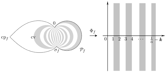
Figure 1. The domain $\mathcal{P}_{f}$ and the Fatou coordinate $\Phi_{f}$. The image of $\mathcal{P}_{f}$ under $\Phi_{f}$ has been coloured accordingly by the same color on the right.

The statement of Proposition 4.1 in [IS06] is in another form. One can refer to Main Theorems 1 and 3 there for further details. See [BC12, Proposition 12] for the present form of Proposition 4.1 (see also [Che19, Proposition 2.4]). The map $\Phi_{f}$ is called the (perturbed) Fatou coordinate and $\mathcal{P}_{f}$ is called a (perturbed) petal.

4.2. Near-parabolic renormalization

Let $f\in\mathcal{IS}_{\alpha}\cup\{Q_{\alpha}\}$ with $\alpha\in(0,r_{1}]$, where $r_{1}>0$ is the constant introduced in Proposition 4.1. Define

(4.8) $$\begin{split}\mathcal{C}_{f}=&\,\{z\in\mathcal{P}_{f}:1/2\leq\textup{Re\,}\Phi_{f}(z)\leq 3/2\text{\leavevmode\nobreak\ and\leavevmode\nobreak\ }-2<\textup{Im\,}\Phi_{f}(z)\leq 2\},\text{\leavevmode\nobreak\ and}\\ \mathcal{C}_{f}^{\sharp}=&\,\{z\in\mathcal{P}_{f}:1/2\leq\textup{Re\,}\Phi_{f}(z)\leq 3/2\text{\leavevmode\nobreak\ and\leavevmode\nobreak\ }2\leq\textup{Im\,}\Phi_{f}(z)\}.\end{split}$$

Note that $\textup{cv}=-4/27\in\operatorname{int}\,\mathcal{C}_{f}$ and $0\in\partial\mathcal{C}_{f}^{\sharp}$. Assume for the moment that there exists an integer $k_{f}\geq 1$, depending on $f$, with the following properties:

1. For all $1\leq k\leq k_{f}$, there is a unique component $(\mathcal{C}_{f}^{\sharp})^{-k}$ of $f^{-k}(\mathcal{C}_{f}^{\sharp})$ containing $0$ in its closure such that $f^{\circ k}:(\mathcal{C}_{f}^{\sharp})^{-k}\to\mathcal{C}_{f}^{\sharp}$ is an isomorphism;

2. There is a unique component $\mathcal{C}_{f}^{-k}$ of $f^{-k}(\mathcal{C}_{f})$ intersecting $(\mathcal{C}_{f}^{\sharp})^{-k}$ such that $f^{\circ k}:\mathcal{C}_{f}^{-k}\to\mathcal{C}_{f}$ is a covering of degree two ramified above cv.

3. $\mathcal{C}_{f}^{-k_{f}}\cup(\mathcal{C}_{f}^{\sharp})^{-k_{f}}$ is contained in $\{z\in\mathcal{P}_{f}:1/2<\textup{Re\,}\Phi_{f}(z)<\alpha^{-1}-\textit{{k}}-1/2\}$.

Moreover, for all $k=1$, $\cdots$, $k_{f}$, the set $(\mathcal{C}_{f})^{-k}\cup(\mathcal{C}_{f}^{\sharp})^{-k}$ is compactly contained in $U_{f}$.

Let $k_{f}$ be the smallest positive integer satisfying the above properties. We now give the definition of near-parabolic renormalization.

Definition 4.2 (Near-parabolic renormalization, see Figure 2).

Define

(4.9) $$S_{f}=\mathcal{C}_{f}^{-k_{f}}\cup(\mathcal{C}_{f}^{\sharp})^{-k_{f}},$$

and consider the map

(4.10) $$\Phi_{f}\circ f^{\circ k_{f}}\circ\Phi_{f}^{-1}:\Phi_{f}(S_{f})\to\mathbb{C}.$$

This map commutes with the translation by one. Hence it projects by the modified exponential map

(4.11) $$\mathbb{E}\textup{xp}(\zeta)=-\tfrac{4}{27}\,e^{2\pi\textup{i}\zeta}$$

to a well-defined map $\mathcal{R}f$ which is defined on a set punctured at zero. One can check that $\mathcal{R}f$ extends across zero and satisfies $\mathcal{R}f(0)=0$ and $(\mathcal{R}f)^{\prime}(0)=e^{-2\pi\textup{i}/\alpha}$. The map $\mathcal{R}f$, restricted to the interior of $\mathbb{E}\textup{xp}(\Phi_{f}(S_{f}))$, is called the near-parabolic renormalization of $f$.

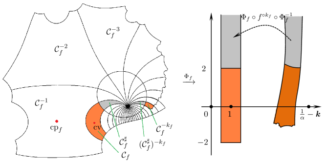
Figure 2. The sets $\mathcal{C}_{f}$, $\mathcal{C}_{f}^{\sharp}$ and some of their preimages. The images of $\mathcal{C}_{f}\cup\mathcal{C}_{f}^{\sharp}$ and $S_{f}$ under the perturbed Fatou coordinate $\Phi_{f}$ have been shown and the induced map $\Phi_{f}\circ f^{\circ k_{f}}\circ\Phi_{f}^{-1}$ projects to the near-parabolic renormalization map $\mathcal{R}f$ under the modified exponential map $\mathbb{E}\textup{xp}$.

Recall that $P(z)=z(1+z)^{2}$ is the cubic polynomial defined at the beginning of the last subsection. Define

(4.12) $$U^{\prime}=P^{-1}(\mathbb{D}(0,\tfrac{4}{27}e^{4\pi}))\setminus((-\infty,-1]\cup\overline{B}),$$

where $B$ is the connected component of $P^{-1}(\mathbb{D}(0,\frac{4}{27}e^{-4\pi}))$ containing $-1$. By an explicit calculation, one can prove that $\overline{U}\subset U^{\prime}$ (see [IS06, Proposition 5.2]).

Theorem 4.3 ([IS06, Main Theorem 3]).

For all $f\in\mathcal{IS}_{\alpha}\cup\{Q_{\alpha}\}$ with $\alpha\in(0,r_{1}]$, the renormalization map $\mathcal{R}f$ is well-defined so that $\mathcal{R}f=P\circ\psi^{-1}\in\mathcal{IS}_{-1/\alpha}$ and $\psi$ extends to a univalent function from $U^{\prime}$ to $\mathbb{C}$.

For $f\in\mathcal{IS}_{\alpha}\cup\{Q_{\alpha}\}$ with $\alpha\in[-r_{1},0)$, the conjugated map $\widetilde{f}=s\circ f\circ s$ satisfies $\widetilde{f}(0)=0$ and $\widetilde{f}^{\prime}(0)=e^{2\pi\textup{i}(-\alpha)}$, where $s:z\mapsto\overline{z}$ is the complex conjugacy. According to the structure of $\mathcal{IS}_{0}$ ($U$ is symmetric about the real axis), we know that $\mathcal{IS}_{0}$ is invariant under complex conjugacy and $\widetilde{f}\in\mathcal{IS}_{-\alpha}\cup\{Q_{-\alpha}\}$. Hence we can extend the domain of definition of the near-parabolic renormalization operator $\mathcal{R}$ to $f\in\mathcal{IS}_{\alpha}\cup\{Q_{\alpha}\}$ with $\alpha\in[-r_{1},0)\cup(0,r_{1}]$.

The following result shows that $k_{f}$ has a uniform upper bound which is independent of $f$.

Proposition 4.4 ([Che19, Proposition 2.7]).

There exists an integer $\textit{{k}}_{1}\geq 1$ such that for all $f\in\mathcal{IS}_{\alpha}\cup\{Q_{\alpha}\}$ with $\alpha\in(0,r_{1}]$, then $k_{f}\leq\textit{{k}}_{1}$.

For another proof of Proposition 4.4, see [BC12, Proposition 13]. For the corresponding statements of Propositions 4.1 and 4.4 with $\alpha\in\mathbb{C}$ (specifically, $|\arg\alpha|<\pi/4$ and $|\alpha|$ is small), see [CS15, Section 2].

4.3. Renormalization tower

Let $f\in\mathcal{IS}_{\alpha}\cup\{Q_{\alpha}\}$ with $\alpha=[(a_{-1},\varepsilon_{0})$; $(a_{0},\varepsilon_{1})$, $\cdots$, $(a_{n},\varepsilon_{n+1})$, $\cdots]\in\textup{HT}_{N}$, where $N\geq 1/r_{1}+1/2$. Recall that $s(z)=\overline{z}$. We define

(4.13) $$f_{0}=\left\{\begin{aligned} &f&\leavevmode\nobreak\ \leavevmode\nobreak\ \leavevmode\nobreak\ \text{if}&\quad\varepsilon_{0}=+1,\\ &s\circ f\circ s&\leavevmode\nobreak\ \leavevmode\nobreak\ \leavevmode\nobreak\ \text{if}&\quad\varepsilon_{0}=-1.\end{aligned}\right.$$

Then the rotation number of $f_{0}$ at the origin belongs to $(0,r_{1}]$. By (2.3), for all $n\in\mathbb{N}$ one has 

(4.14) $$\alpha_{n}^{-1}=a_{n}+\varepsilon_{n+1}\alpha_{n+1}\geq N-1/2\geq 1/r_{1}.$$

By Theorem 4.3, for $n\geq 1$, the following sequence of maps can be defined inductively:

(4.15) $$f_{n}=\left\{\begin{aligned} &\mathcal{R}(f_{n-1})&\leavevmode\nobreak\ \leavevmode\nobreak\ \leavevmode\nobreak\ \text{if}&\quad\varepsilon_{n}=-1,\\ &s\circ\mathcal{R}(f_{n-1})\circ s&\leavevmode\nobreak\ \leavevmode\nobreak\ \leavevmode\nobreak\ \text{if}&\quad\varepsilon_{n}=+1.\end{aligned}\right.$$

Let $U_{n}=U_{f_{n}}$ be the domain of definition of $f_{n}$ for $n\geq 0$. Then for all $n\geq 1$, we have

(4.16) $$f_{n}\in\mathcal{IS}_{\alpha_{n}},\leavevmode\nobreak\ f_{n}:U_{n}\to\mathbb{C},\leavevmode\nobreak\ f_{n}(0)=0,\leavevmode\nobreak\ f_{n}^{\prime}(0)=e^{2\pi\textup{i}\alpha_{n}}\text{\leavevmode\nobreak\ and\leavevmode\nobreak\ }\textup{cv}_{f_{n}}=-4/27.$$

For $n\geq 0$, let $\Phi_{n}=\Phi_{f_{n}}$ be the Fatou coordinate of $f_{n}:U_{n}\to\mathbb{C}$ defined on the petal $\mathcal{P}_{n}=\mathcal{P}_{f_{n}}$ and let $\mathcal{C}_{n}=\mathcal{C}_{f_{n}}$ and $\mathcal{C}_{n}^{\sharp}=\mathcal{C}_{f_{n}}^{\sharp}$ be the corresponding sets for $f_{n}$ defined in (4.8). Let $k_{n}=k_{f_{n}}$ be the smallest integer appeared in the definition of the renormalization operator $\mathcal{R}$ such that

(4.17) $$S_{n}=\mathcal{C}_{n}^{-k_{n}}\cup(\mathcal{C}_{n}^{\sharp})^{-k_{n}}\subset\{z\in\mathcal{P}_{n}:1/2<\textup{Re\,}\Phi_{n}(z)<\alpha_{n}^{-1}-\textit{{k}}-1/2\}.$$

We use $\sigma_{n}=\sigma_{f_{n}}$ to denote the non-zero fixed point of $f_{n}$ on the boundary of $\mathcal{P}_{n}$. It is known that $|\sigma_{n}|$ is comparable to $\alpha_{n}$ and the comparable constants are independent of $n$ (see [CS15, Equation (14)]).

4.4. Changes of the coordinates

Recall that the integer part of $x>0$ is denoted by ${\lfloor{x}\rfloor}\in(x-1,x]$. For $n\geq 0$, we denote

(4.18) $$\begin{split}\Pi_{n}=&\leavevmode\nobreak\ \{\zeta\in\mathbb{C}:-1/(2\alpha_{n})\leq\textup{Re\,}\zeta<0,\,\textup{Im\,}\zeta>0\}\\ &\leavevmode\nobreak\ \cup\Phi_{n}(\mathcal{P}_{n})\cup\bigcup_{i=0}^{k_{n}+{\lfloor{1/(2\alpha_{n})}\rfloor}}(\Phi_{n}(S_{n})+i).\end{split}$$

The univalent map $\Phi_{n}^{-1}:\Phi_{n}(\mathcal{P}_{n})\to\mathcal{P}_{n}$ can be extended to a holomorphic map

(4.19) $$\Phi_{n}^{-1}:\Pi_{n}\to U_{n}\setminus\{0\}$$

such that $\Phi_{n}^{-1}(\zeta+1)=f_{n}\circ\Phi_{n}^{-1}(\zeta)$ if $\zeta$, $\zeta+1\in\Pi_{n}$. Note that the exponential map $\mathbb{E}\textup{xp}:\mathbb{C}\to\mathbb{C}\setminus\{0\}$ is a covering map. Recall that $s(z)=\overline{z}$. The maps $\Phi_{n}^{-1}:\Pi_{n}\to\mathbb{C}\setminus\{0\}$ and $s\circ\Phi_{n}^{-1}:\Pi_{n}\to\mathbb{C}\setminus\{0\}$ can be lifted to obtain a holomorphic or an anti-holomorphic map $\chi_{n}:\Pi_{n}\to\mathbb{C}$ such that

(4.20) $$\forall\zeta\in\Pi_{n},\quad\left\{\begin{aligned} &\mathbb{E}\textup{xp}\circ\chi_{n}(\zeta)=\Phi_{n}^{-1}(\zeta)&\leavevmode\nobreak\ \leavevmode\nobreak\ \leavevmode\nobreak\ \text{if}&\quad\varepsilon_{n}=-1,\\ &\mathbb{E}\textup{xp}\circ\chi_{n}(\zeta)=s\circ\Phi_{n}^{-1}(\zeta)&\leavevmode\nobreak\ \leavevmode\nobreak\ \leavevmode\nobreak\ \text{if}&\quad\varepsilon_{n}=+1.\end{aligned}\right.$$

The map $\chi_{n}$ is holomorphic if $\varepsilon_{n}=-1$ while it is anti-holomorphic if $\varepsilon_{n}=+1$. Moreover, $\chi_{n}:\Pi_{n}\to\mathbb{C}$ is an injection and we assume that $\chi_{n}$ is chosen so that 

(4.21) $$\chi_{n}(1)=1.$$

For $j\in\mathbb{Z}$ we define

(4.22) $$\chi_{n,j}=\chi_{n}+j.$$

4.5. Some estimates on the changes of coordinates

Recall that $\sigma_{n}\neq 0$ is another fixed point of $f_{n}$ near $0$ which is contained in $\partial\mathcal{P}_{n}$. Let

(4.23) $$\tau_{n}(w)=\frac{\sigma_{n}}{1-e^{-2\pi\textup{i}\alpha_{n}w}}$$

be a universal covering from $\mathbb{C}$ to $\widehat{\mathbb{C}}\setminus\{0,\sigma_{n}\}$ with period $1/\alpha_{n}$. Then $\tau_{n}(w)\to 0$ as $\textup{Im\,}w\to+\infty$ and $\tau_{n}(w)\to\sigma_{n}$ as $\textup{Im\,}w\to-\infty$. The basic idea to study the Fatou coordinate $\Phi_{n}$ is to compare the inverse $\Phi_{n}^{-1}$ with $\tau_{n}$. There exists a unique lift $F_{n}$ of $f_{n}$ under $\tau_{n}$ such that

(4.24) $$f_{n}\circ\tau_{n}(w)=\tau_{n}\circ F_{n}(w)\text{ with }\lim_{\textup{Im\,}w\to+\infty}(F_{n}(w)-w)=1.$$

Since the critical points of $F_{n}$ are periodic with period $1/\alpha_{n}$. We use $\widetilde{\textup{cp}}_{n}$ to denote the one which is closest to the origin. The set $\tau_{n}^{-1}(\mathcal{P}_{n})$ has countably many simply connected components. Each of these components is bounded by piecewise analytic curves going from $-\textup{i}\infty$ to $+\textup{i}\infty$ and it contains a unique critical point of $F_{n}$ on its boundary. Let $\widetilde{\mathcal{P}}_{n}$ be the component containing $\widetilde{\textup{cp}}_{n}$ on its boundary. Define the univalent map

(4.25) $$L_{n}=\Phi_{n}\circ\tau_{n}:\widetilde{\mathcal{P}}_{n}\to\mathbb{C}.$$

This map is the Fatou coordinate of $F_{n}$ since $L_{n}\circ F_{n}(w)=L_{n}(w)+1$ when $w$ and $F_{n}(w)$ are both contained in $\widetilde{\mathcal{P}}_{n}$.

The inverse $L_{n}^{-1}:\Phi_{n}(\mathcal{P}_{n})\to\widetilde{\mathcal{P}}_{n}$ can be extended to a holomorphic function on a larger domain $\Pi_{n}$ (see (4.18) and [Che19, Section 6]). The main work on $L_{n}^{-1}$ in [Che19, Section 6] is to establish some quantitative distance estimates between $L_{n}^{-1}$ and the identity. For more details on the study of $L_{n}$ and $L_{n}^{-1}$, see [Che19, Sections 6.3-6.6] and [CS15, Section 3.5]. The following Lemma 4.5 and Proposition 4.6 are obtained from studying $L_{n}^{-1}$ and a direct calculation.

Lemma 4.5 ([SY18, Lemma 2.11]).

For all $D_{0}>0$, there exists two constants $M_{0}$, $\widetilde{M}_{0}>0$ such that for all $n\geq 1$, we have

1. If $\zeta\in\Pi_{n}$ with $\textup{Im\,}\zeta\geq D_{0}/\alpha_{n}$, then

   (4.26) $$\Big{|}\textup{Im\,}\chi_{n}(\zeta)-\Big{(}\alpha_{n}\,\textup{Im\,}\zeta+\frac{1}{2\pi}\log\frac{1}{\alpha_{n}}\Big{)}\Big{|}\leq M_{0}.$$

2. If $\zeta\in\Pi_{n}$ with $\textup{Im\,}\zeta\in[-2,D_{0}/\alpha_{n}]$, then

   (4.27) $$\Big{|}\textup{Im\,}\chi_{n}(\zeta)-\tfrac{1}{2\pi}\min\big{\{}\log(1+|\zeta|),\log(1+|\zeta-1/\alpha_{n}|)\big{\}}\Big{|}\leq\widetilde{M}_{0}.$$

Note that $M_{0}>0$ in Lemma 4.5(a) can be chosen such that it decreases as $D_{0}$ increases. Partial estimation of Lemma 4.5 can be also found in [Che19, Proposition 5.4]. When one applies $\chi_{n}:\Pi_{n}\to\mathbb{C}$, Lemma 4.5 gives an estimation on the imaginary part of $\chi_{n}(\zeta)$ for $\zeta\in\Pi_{n}\cap\{\zeta\in\mathbb{C}:\textup{Im\,}\zeta\geq-2\}$. We will use the following result to study the real part of $\chi_{n}(\zeta)$ for some $\zeta\in\Pi_{n}$ and estimate the diameter of some boxes when we go up the renormalization tower (see Section 5).

Proposition 4.6 ([Che13, Che19]).

For all $D_{0}>0$, there exists two constants $M_{1}$, $\widetilde{M}_{1}\geq 1$ such that for all $n\geq 1$, we have

1. If $\zeta\in\Pi_{n}\cap\{\zeta:\textup{Im\,}\zeta\geq-2\}$ with $|\zeta|\geq D_{0}/\alpha_{n}$ and $|\zeta-1/\alpha_{n}|\geq D_{0}/\alpha_{n}$, then

   (4.28) $$|\chi_{n}^{\prime}(\zeta)-\alpha_{n}|\leq M_{1}\alpha_{n}e^{-2\pi\alpha_{n}\textup{Im\,}\zeta}.$$

2. If $\zeta\in\Pi_{n}\cap\{\zeta:\textup{Im\,}\zeta\geq-2\}$ with $1\leq|\zeta|<D_{0}/\alpha_{n}$ or $1\leq|\zeta-1/\alpha_{n}|<D_{0}/\alpha_{n}$, then

   (4.29) $$\widetilde{M}_{1}^{-1}\leq\min\{|\zeta|,|\zeta-1/\alpha_{n}|\}\cdot|\chi_{n}^{\prime}(\zeta)|\leq\widetilde{M}_{1}.$$

Similar to Lemma 4.5(a), the number $M_{1}>0$ in Proposition 4.6(a) can be chosen such that it decreases as $D_{0}$ increases. Proposition 4.6(a) is proved in [Che13, Proposition 3.3]. Actually, the latter proves a stronger statement where the dependence of $M_{1}$ on $D_{0}$ is established and the inequality holds in a larger domain. Proposition 4.6(b) is proved in [Che19, Proposition 6.18] for $\zeta\in[1,1/(2\alpha_{n})]$ (i.e., $\zeta\in\mathbb{R}$). However, the proof for the complex $\zeta$ is completely similar. See also [SY18, Proposition 2.13(b)] for a more elaborate estimation for case (b).

In the rest of this article, for a given map $f=f_{0}\in\mathcal{IS}_{\alpha}\cup\{Q_{\alpha}\}$ with $\alpha\in\textup{HT}_{N}$, where $N\geq 1/r_{1}+1/2$, we use $f_{n}$ to denote the map after $n$-th (normalized) near-parabolic renormalization. We also use $U_{n}$, $\mathcal{P}_{n}$ and $\Phi_{n}$ etc to denote the domain of definition, perturbed petal and the Fatou coordinate etc of $f_{n}$ respectively.

For some recent remarkable applications of near-parabolic renormalization scheme one may refer to [CC15], [CS15], [AL15], [CP17] etc. Recently, Chéritat generalized the near-parabolic theory to all the unicritical case for any finite degrees [Che14]. See also [Yan15] for the corresponding theory of local degree three. Therefore, there is a hope to generalize the results in this paper to all unicritical polynomials.

5. Almost rectagular partition of the post-critical sets

In this section, we first recall two results on the topological structure of the post-critical set $\Lambda_{f}$ of $f\in\mathcal{IS}_{\alpha}\cup\{Q_{\alpha}\}$ with $\alpha\in\textup{HT}_{N}$. Then we define a system satisfying the nesting conditions and use some estimations between the renormalization levels to estimate the densities and the diameters of some related sets. In next section we use the criterion established in Section 3 to obtain the full Hausdorff dimension of $\Lambda_{f}$ under the assumption that $\alpha\in\textup{HT}_{N}\setminus\mathscr{H}$.

5.1. Topology of the post-critical sets

A Cantor bouquet is a compact subset of the plane which is homeomorphic to a set of the form

(5.1) $$\{re^{2\pi i\theta}\in\mathbb{C}\mid 0\leq r\leq R(\theta)\}$$

where $R:\mathbb{R}/\mathbb{Z}\to[0,\infty)$ satisfies

• $R^{-1}(0)$ is dense in $\mathbb{R}/\mathbb{Z}$,

• $(\mathbb{R}/\mathbb{Z})\setminus R^{-1}(0)$ is dense in $\mathbb{R}/\mathbb{Z}$,

• for each $\theta_{0}\in\mathbb{R}/\mathbb{Z}$ we have

  $$\limsup_{\theta\to\theta_{0}^{+}}R(\theta)=R(\theta_{0})=\limsup_{\theta\to\theta_{0}^{-}}R(\theta).$$

A one-sided hairy Jordan curve is a compact subset of the plane which is homeomorphic to a set of the form

(5.2) $$\{re^{2\pi i\theta}\in\mathbb{C}\mid 1\leq r\leq R(\theta)\}$$

where $R:\mathbb{R}/\mathbb{Z}\to[1,\infty)$ satisfies

• $R^{-1}(1)$ is dense in $\mathbb{R}/\mathbb{Z}$,

• $(\mathbb{R}/\mathbb{Z})\setminus R^{-1}(1)$ is dense in $\mathbb{R}/\mathbb{Z}$,

• for each $\theta_{0}\in\mathbb{R}/\mathbb{Z}$ we have

  $$\limsup_{\theta\to\theta_{0}^{+}}R(\theta)=R(\theta_{0})=\limsup_{\theta\to\theta_{0}^{-}}R(\theta).$$

Let $N\geq 1/r_{1}+1/2$. In order to study the Hausdorff dimension of $\Lambda_{f}$, we also need some topological properties of $\Lambda_{f}$.

Theorem 5.1 (Trilogy of the postcritical set [Che17]).

Let $f\in\mathcal{IS}_{\alpha}\cup\{Q_{\alpha}\}$ with $\alpha\in\textup{HT}_{N}$. Then

• if $\alpha\in\mathscr{H}$, $\Lambda(f)$ is a Jordan curve;

• if $\alpha\in\mathscr{B}\setminus\mathscr{H}$, then $\Lambda_{f}$ is a one-sided hairy circle, and the connected component of $\Lambda_{f}\setminus\overline{\Delta}_{f}$ containing the critical value of $f$ is a $C^{1}$ curve;

• if $\alpha\not\in\mathscr{B}$, then $\Lambda_{f}$ is a Cantor bouquet, and the connected component of $\Lambda_{f}\setminus\{0\}$ containing the critical value of $f$ is a $C^{1}$ curve.

For the definitions of Cantor bouquet and one-sided hairy circle, one may refer to [Che17]. In particular, each connected component of $\Lambda_{f}\setminus\overline{\Delta}_{f}$ is a Jordan arc, where $\Delta_{f}$ is the Siegel disk of $f$ if $\alpha\in\mathscr{B}\setminus\mathscr{H}$ while $\overline{\Delta}_{f}=\{0\}$ is the Cremer point if $\alpha\not\in\mathscr{B}$.

Definition 5.2 (Critical value curve).

For $f\in\mathcal{IS}_{\alpha}\cup\{Q_{\alpha}\}$ with $\alpha\in\textup{HT}_{N}$, let $\Gamma_{f}$ be the Jordan arc connecting the critical value $\textup{cv}=-4/27$ with the origin (not including $0$) stated in Theorem 5.1. The arc $\Gamma_{f}$ is called the critical value curve. It is known that $\Gamma_{f}\subset\mathcal{P}_{f}$, where $\mathcal{P}_{f}$ is the perturbed petal of $f$. More precisely, following [Che17, Lemma 3.4] or [SY18, Proposition 5.3], we have

(5.3) $$\gamma_{f}=\Phi_{f}(\Gamma_{f})\subset\mho=\{\zeta\in\mathbb{C}:1/2<\textup{Re\,}\zeta<3/2\text{ and }\textup{Im\,}\zeta>-2\}.$$

We also call $\gamma_{f}$ the critical value curve in the Fatou coordinate plane of $f$. Let $\gamma_{f}^{\prime}\subset\Phi_{f}(S_{f})+k_{f}$ be the simple arc such that $\Phi_{f}^{-1}(\gamma_{f}^{\prime})=\Gamma_{f}$.

Theorem B in [Che17] states that the real part of $\gamma_{f}$ (resp. $\gamma_{f}^{\prime}$) tends to a limit as the imaginary part tends to positive infinity. Indeed, the following result shows that the curves $\gamma_{f}$ and $\gamma_{f}^{\prime}$ become more and more straight as the imaginary part increases.

Proposition 5.3 ([Che17, Lemmas 4.11 and 4.13]).

For any $\varepsilon>0$, there exists a constant $\widetilde{M}_{2}=\widetilde{M}_{2}(\varepsilon)>0$ such that for all $f\in\mathcal{IS}_{\alpha}\cup\{Q_{\alpha}\}$ with $\alpha\in\textup{HT}_{N}$, if $\zeta$, $\zeta^{\prime}\in\gamma_{f}$ (or $\gamma_{f}^{\prime}$) with $\textup{Im\,}\zeta>\textup{Im\,}\zeta^{\prime}\geq\widetilde{M}_{2}$, then

(5.4) $$|\arg(\zeta-\zeta^{\prime})-\pi/2|<\varepsilon.$$

For $y\in\mathbb{R}$, we define

(5.5) $$\mathbb{L}_{y}=\{z\in\mathbb{C}:\textup{Im\,}z=y\}\text{\quad and\quad}\mathbb{H}_{y}=\{z\in\mathbb{C}:\textup{Im\,}z\geq y\}.$$

By Proposition 5.3, we have the following immediate corollary.

Corollary 5.4.

There exists a constant $D_{2}^{\prime}\geq 1$ such that for all $f\in\mathcal{IS}_{\alpha}\cup\{Q_{\alpha}\}$ with $\alpha\in\textup{HT}_{N}$ and for all $y\geq D_{2}^{\prime}$, then

(5.6) $$\mathbb{L}_{y}\cap(\gamma_{f}+j)\text{ and }\mathbb{L}_{y}\cap(\gamma_{f}^{\prime}+j)$$

are both singletons for all $j\in\mathbb{Z}$.

As before, let $f_{n}$ be the map after $n$-th (normalized) near-parabolic renormalization of a given map $f\in\mathcal{IS}_{\alpha}\cup\{Q_{\alpha}\}$ with $\alpha\in\textup{HT}_{N}$. We use $\Gamma_{n}$, $\gamma_{n}$ and $\gamma_{n}^{\prime}$ etc to denote the simple arcs introduced above.

5.2. Going down the renormalization tower

For each $n\geq 0$, from the definition of $\gamma_{n}$ and $\gamma_{n}^{\prime}$ we have $\Phi_{n}^{-1}(\gamma_{n})=\Gamma_{n}=\Phi_{n}^{-1}(\gamma_{n}^{\prime})$. Recall that $\mho$ is an half-infinite trip defined in (5.3). For $n\geq 1$ and $j\in\mathbb{Z}$ we have

(5.7) $$\Phi_{n}\circ\mathbb{E}\textup{xp}(\gamma_{n-1}+j)=\Phi_{n}(\Gamma_{n})=\gamma_{n}\subset\mho.$$

Recall that $D_{2}^{\prime}\geq 1$ is the constant introduced in Corollary 5.4. For all $n\geq 0$, we define

(5.8) $$Y_{n}=Y_{n}(D_{2}^{\prime})=\left\{\begin{array}[]{l}\text{The closure of the connected component of}\\ \mathbb{C}\setminus(\gamma_{n}\cup\gamma_{n}^{\prime}\cup\mathbb{L}_{D_{2}^{\prime}})\text{ containing }2+(D_{2}^{\prime}+1)\,\textup{i}\end{array}\right\}\setminus\gamma_{n}^{\prime}.$$

Then $Y_{n}$ is simply connected and very ‘close’ to a half-infinite strip with width $1/\alpha_{n}$ and it is ‘bottom left’ closed and ‘right’ open. We use $Y_{n,0}\subset Y_{n}$ to denote the ‘bottom left’ closed and ‘right’ open domain bounded by $\gamma_{n}$, $\gamma_{n}+1$ and $\mathbb{L}_{D_{2}^{\prime}}$:

(5.9) $$Y_{n,0}=Y_{n,0}(D_{2}^{\prime})=\left\{\begin{array}[]{l}\text{The closure of the connected component of}\\ \mathbb{C}\setminus(\gamma_{n}\cup(\gamma_{n}+1)\cup\mathbb{L}_{D_{2}^{\prime}})\text{ containing }2+(D_{2}^{\prime}+1)\,\textup{i}\end{array}\right\}\setminus(\gamma_{n}+1).$$

For $j\in\mathbb{Z}$, we denote

(5.10) $$Y_{n,j}=Y_{n,0}+j.$$

By (2.3), if $\varepsilon_{n+1}=-1$, then $a_{n}-1/2<1/\alpha_{n}<a_{n}$. If $\varepsilon_{n+1}=+1$, then $a_{n}<1/\alpha_{n}<a_{n}+1/2$. For $n\in\mathbb{N}$, we define an index set

(5.11) $$\mathbb{J}_{n}=\left\{j\in\mathbb{N}:0\leq j\leq J_{n}-1\right\}\text{\quad with\quad}J_{n}=a_{n}+\tfrac{\varepsilon_{n+1}-1}{2}$$

and a half-infinite strip (see Figure 3)

(5.12) $$Y_{n,*}=Y_{n}\setminus\bigcup_{j\in\mathbb{J}_{n}}Y_{n,j}.$$

Note that $\overline{Y}_{n,*}\subset Y_{n,J_{n}}$.

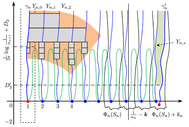
Figure 3. Some sets in the Fatou coordinate plane of $f_{n}$. The critical value curve $\gamma_{n}$, its translations and $\gamma_{n}^{\prime}$ have been drawn. Some useful heights are marked. Moreover, several packed boxes are also shown (in gray, see Section 5.3).

For $n\geq 0$, we define

(5.13) $$Y_{n,\diamond}=\left\{\begin{array}[]{l}\text{The closure of the component of }\mathbb{C}\setminus(\gamma_{n}^{\prime}\cup(\gamma_{n}^{\prime}-1)\cup\mathbb{L}_{D_{2}^{\prime}})\\ \text{which is contained in }\bigcup_{j=-1}^{0}(\Phi_{n}(S_{n})+k_{n}+j)\end{array}\right\}\setminus\gamma_{n}^{\prime}.$$

Note that all the sets $Y_{n}$, $Y_{n,j}$, $Y_{n,*}$ and $Y_{n,\diamond}$ depend on the given height $D_{2}^{\prime}\geq 1$. Recall that $\Pi_{n}$ is defined in (4.18) and we have $\overline{Y}_{n}\subset\Pi_{n}$. Therefore, $\chi_{n,j}$ is well defined on $\overline{Y}_{n}$ for all $j\in\mathbb{Z}$. See Section 4.4 for the definition of $\chi_{n,j}$.

Lemma 5.5.

There is a number $D_{2}>0$ such that for all $n\geq 1$ and $y_{n-1}=\tfrac{1}{2\pi}\log\tfrac{1}{\alpha_{n}}+D_{2}$, we have

1. If $\varepsilon_{n}=-1$, for all $j\in\mathbb{J}_{n-1}$ then

   (5.14) $$\chi_{n,j}(Y_{n})\cap\mathbb{H}_{y_{n-1}}=Y_{n-1,j}\cap\mathbb{H}_{y_{n-1}}$$

   and

   (5.15) $$\chi_{n,J_{n-1}}(Y_{n}\setminus Y_{n,\diamond})\cap\mathbb{H}_{y_{n-1}}=Y_{n-1,*}\cap\mathbb{H}_{y_{n-1}}.$$

2. If $\varepsilon_{n}=+1$, for all $j\in\mathbb{J}_{n-1}$ then

   (5.16) $$\chi_{n,j+1}(\overline{Y}_{n}\setminus\gamma_{n})\cap\mathbb{H}_{y_{n-1}}=Y_{n-1,j}\cap\mathbb{H}_{y_{n-1}}$$

   and

   (5.17) $$\chi_{n,J_{n-1}+1}(\overline{Y}_{n,\diamond}\setminus(\gamma_{n}^{\prime}-1))\cap\mathbb{H}_{y_{n-1}}=Y_{n-1,*}\cap\mathbb{H}_{y_{n-1}}.$$

Proof.

We only prove case (a) since the proof of case (b) is completely similar. If $\varepsilon_{n}=-1$ then $\chi_{n}:\Pi_{n}\to\mathbb{C}$ is holomorphic (see (4.20)). The first statement follows from Lemma 4.5 and the facts that $\chi_{n}(\gamma_{n})=\gamma_{n-1}$, $\chi_{n}(\gamma_{n}^{\prime})=\gamma_{n-1}+1$ and the definition of $\chi_{n,j}$ with $j\in\mathbb{J}_{n-1}$.

By the definition of near-parabolic renormalization, we have $f_{n}(\mathbb{E}\textup{xp}(\gamma_{n-1}^{\prime}))=\mathbb{E}\textup{xp}(\gamma_{n-1}+J_{n-1})=\Gamma_{n}$. This means that $\mathbb{E}\textup{xp}(\gamma_{n-1}^{\prime})$ is the critical point curve $\Gamma_{n}^{\textup{cp}}$ of $f_{n}$, i.e., the union of $\textup{cp}_{n}$ and the component of $f_{n}^{-1}(\Gamma_{n}\setminus\{\textup{cv}\})$ with endpoints $0$ and $\textup{cp}_{n}$. If we consider $\Phi_{n}^{-1}:\Pi_{n}\to\mathbb{C}$, it is easy to see that $\Phi_{n}^{-1}(\gamma_{n})=\Gamma_{n}$ and $\Phi_{n}^{-1}(\gamma_{n}^{\prime}-1)=\Gamma_{n}^{\textup{cp}}$. In particular, by Lemma 4.5 if $D_{2}>0$ is large then we have $\chi_{n,J_{n-1}}(Y_{n}\setminus Y_{n,\diamond})\cap\mathbb{H}_{y_{n-1}}=Y_{n-1,*}\cap\mathbb{H}_{y_{n-1}}$. ∎

Remark.

In the case $\varepsilon_{n}=-1$, the images of $Y_{n}$ under $\chi_{n,j}$ with $j\in\mathbb{J}_{n-1}$, and the union of the image of $Y_{n}\setminus Y_{n,\diamond}$ under $\chi_{n,J_{n-1}}$ will cover the whole upper end of $Y_{n-1}$ since

(5.18) $$\Big{(}Y_{n-1,*}\cup\bigcup_{j\in\mathbb{J}_{n-1}}Y_{n-1,j}\Big{)}\cap\mathbb{H}_{y_{n-1}}=Y_{n-1}\cap\mathbb{H}_{y_{n-1}}.$$

One can have the similar observation for $\varepsilon_{n}=+1$.

In order to simplify notations, for $n\geq 1$ and $j\in\mathbb{Z}$, we denote by

(5.19) $$\chi_{n,*}=\chi_{n,J_{n-1}}\text{\quad and\quad}\chi_{n,*+j}=\chi_{n,J_{n-1}+j}.$$

For $n\geq 1$, we define (compare Lemma 5.5):

(5.20) $$X_{n-1}=\left\{\begin{aligned} &\bigcup_{j\in\mathbb{J}_{n-1}\cup\{*\}}\big{(}\chi_{n,j}(Y_{n})\cap Y_{n-1,j}\big{)}&\leavevmode\nobreak\ \leavevmode\nobreak\ \leavevmode\nobreak\ \text{if}&\quad\varepsilon_{n}=-1,\\ &\bigcup_{j\in\mathbb{J}_{n-1}\cup\{*\}}\big{(}\chi_{n,j+1}(\overline{Y}_{n})\cap Y_{n-1,j})\big{)}&\leavevmode\nobreak\ \leavevmode\nobreak\ \leavevmode\nobreak\ \text{if}&\quad\varepsilon_{n}=+1.\end{aligned}\right.$$

It is straightforward to verify that $X_{n-1}$ is connected. Note that the restriction of $\chi_{n,j}$ on $\overline{Y}_{n}$ is injective for every $j\in\mathbb{Z}$.

Definition 5.6 (The inverse of $\chi_{n,j}$).

For $n\geq 1$, we define a map $\xi_{n}:X_{n-1}\to Y_{n}$, which is the inverse of $\chi_{n,j}$, as following:

• if $\varepsilon_{n}=-1$, for $\zeta\in\chi_{n,j}(Y_{n})\cap Y_{n-1,j}$ with $j\in\mathbb{J}_{n-1}\cup\{*\}$, define

  (5.21) $$\xi_{n}(\zeta)=\chi_{n,j}^{-1}(\zeta).$$

• if $\varepsilon_{n}=+1$, for $j\in\mathbb{J}_{n-1}\cup\{*\}$, define

  (5.22) $$\xi_{n}(\zeta)=\left\{\begin{aligned} &\chi_{n,0}^{-1}(\zeta)&\leavevmode\nobreak\ \leavevmode\nobreak\ \leavevmode\nobreak\ \text{if}&\quad\zeta\in\chi_{n,1}(\overline{Y}_{n})\cap\gamma_{n-1},\\ &\chi_{n,j+1}^{-1}(\zeta)&\leavevmode\nobreak\ \leavevmode\nobreak\ \leavevmode\nobreak\ \text{if}&\quad\zeta\in\chi_{n,j+1}(\overline{Y}_{n})\setminus(\gamma_{n-1}+j).\end{aligned}\right.$$

By definition, the map $\xi_{n}:X_{n-1}\to Y_{n}$ is a periodic function with period one. However, it is not continuous on the arc $(\gamma_{n-1}+j)\cap X_{n-1}$, where $1\leq j\leq J_{n-1}$. For example, $\zeta\in(\gamma_{n-1}+1)\cap X_{n-1}$ is a boundary point of $Y_{n-1,0}$ and is also a boundary point of $Y_{n-1,1}$. If $\varepsilon_{n}=-1$, then by definition we have $\xi_{n}(\zeta)\in\gamma_{n}$. But there exists a sequence $(\zeta_{k})_{k\in\mathbb{N}}\subset Y_{n-1,0}$ which converges to $\zeta$ such that $\xi_{n}(\zeta_{k})$ converges to a point on $\gamma_{n}^{\prime}$ as $k\to\infty$.

We will use $(\chi_{n})_{n\geq 1}$ and $(\xi_{n})_{n\geq 1}$, respectively, to go up and go down the renormalization tower. For $\zeta_{0}\in\mathbb{C}$ and $r>0$, we denote by

(5.23) $$\textup{Box}(\zeta_{0},r)=\{\zeta\in\mathbb{C}:|\textup{Re\,}(\zeta-\zeta_{0})|\leq r\text{ and }|\textup{Im\,}(\zeta-\zeta_{0})|\leq r\}$$

the closed square with center $\zeta_{0}$ and with side length $2r$. For $n\in\mathbb{N}$, recall that $\mathbb{J}_{n}$ is defined in (5.11). For $n\in\mathbb{N}$ we define a new index set

(5.24) $$\widetilde{\mathbb{J}}_{n}=\mathbb{J}_{n}\cup\{J_{n}\}=\{j\in\mathbb{N}:0\leq j\leq J_{n}\}.$$

Usually we use $\mathbb{J}_{n}$ and $\widetilde{\mathbb{J}}_{n}$ to mark the translations of $Y_{n,0}$ and $\gamma_{n}$ respectively. In the following, for unifying notations, for $n\in\mathbb{N}$ we denote

(5.25) $$\gamma_{n}+*=\gamma_{n}^{\prime}\text{\quad and\quad}\gamma_{n}+(*-1)=(\gamma_{n}+*)-1=\gamma_{n}^{\prime}-1.$$

For a set $X\subset\mathbb{C}$ and a number $\delta>0$, let $B_{\delta}(X)=\bigcup_{z\in X}\mathbb{D}(z,\delta)$ be the $\delta$-neighborhood of $X$. Recall that $Y_{n}=Y_{n}(D_{2}^{\prime})$ is a set defined in (5.8). For given positive numbers $D_{3}$, $D_{3}^{\prime}\geq D_{2}^{\prime}$, $\nu\in(0,1/2)$ and all $n\in\mathbb{N}$, we define

(5.26) $$\begin{split}\Xi_{n}=&\leavevmode\nobreak\ \Xi_{n}(D_{3}^{\prime},D_{3},\nu)\\ =&\leavevmode\nobreak\ Y_{n}\big{(}\tfrac{1}{2\pi}\log\tfrac{1}{\alpha_{n+1}}+D_{3}\big{)}\cup\big{(}Y_{n}(D_{3}^{\prime})\cap B_{\nu}(\gamma_{n}+\widetilde{\mathbb{J}}_{n}\cup\{*,*-1\})\big{)}\end{split}$$

and

(5.27) $$\Xi_{n,j}=\Xi_{n}\cap Y_{n,j}(D_{3}^{\prime}),$$

where $j\in\mathbb{J}_{n}\cup\{*\}$. For given $n\in\mathbb{N}$, $D_{3}^{\prime\prime\prime}>D_{3}^{\prime\prime}\geq D_{3}$ and $j\in\mathbb{J}_{n}\cup\{*\}$, we define

(5.28) $$W_{n,j}(D_{3}^{\prime\prime},D_{3}^{\prime\prime\prime})=\{\zeta\in Y_{n,j}:D_{3}^{\prime\prime}\leq\textup{Im\,}\zeta-\tfrac{1}{2\pi}\log\tfrac{1}{\alpha_{n+1}}\leq D_{3}^{\prime\prime\prime}\}.$$

Lemma 5.7.

There exist constants $D_{3}$, $D_{3}^{\prime}\geq D_{2}^{\prime}$ and $\nu_{0}\in(0,1/20]$ such that for all $n\geq 1$, we have

1. $\Xi_{n-1}=\Xi_{n-1}(D_{3}^{\prime},D_{3},\nu_{0})\subset X_{n-1}$;

2. For any $\zeta_{n-1}$, $\zeta_{n-1}^{\prime}\in\Xi_{n-1,j}\cap B_{\nu_{0}}(\gamma_{n-1}+j^{\prime})$ with $\zeta_{n-1}\in\gamma_{n-1}+j^{\prime}$ and $\textup{Im\,}\zeta_{n-1}^{\prime}\geq\textup{Im\,}\zeta_{n-1}-\nu_{0}$, where $j\in\mathbb{J}_{n-1}\cup\{*\}$ and $j^{\prime}\in\widetilde{\mathbb{J}}_{n-1}\cup\{*,*-1\}$, then

   (5.29) $$\textup{Im\,}\xi_{n}(\zeta_{n-1}^{\prime})\geq\tfrac{3}{4}\,\textup{Im\,}\xi_{n}(\zeta_{n-1});$$

3. For $\zeta_{n-1}\in\gamma_{n-1}+j^{\prime}$ such that $\textup{Box}(\zeta_{n-1},\nu_{0})\cap Y_{n-1,j}\neq\emptyset$, where $j\in\mathbb{J}_{n-1}\cup\{*\}$ and $j^{\prime}\in\widetilde{\mathbb{J}}_{n-1}\cup\{*,*-1\}$, $\xi_{n}:\textup{Box}(\zeta_{n-1},\nu_{0})\cap Y_{n-1,j}\to Y_{n}$ can be extended to a univalent (or an anti-univalent) map $\widetilde{\xi}_{n,j}:\textup{Box}(\zeta_{n-1},20\nu_{0})\to\Pi_{n}$;

4. For any $D_{3}^{\prime\prime\prime}>D_{3}^{\prime\prime}\geq D_{3}$, $\xi_{n}:W_{n-1,j}\cap Y_{n-1}\to Y_{n}$ can be extended to a univalent (or an anti-univalent) map $\widetilde{\xi}_{n,j}:B_{\nu_{0}}(W_{n-1,j})\to\Pi_{n}$, where $W_{n-1,j}=W_{n-1,j}(D_{3}^{\prime\prime},D_{3}^{\prime\prime\prime})$ and $j\in\mathbb{J}_{n-1}\cup\{*\}$.

Proof.

We only prove the case $\varepsilon_{n}=-1$ since the proof of the case $\varepsilon_{n}=+1$ is completely similar.

(a) Recall that $D_{2}^{\prime}\geq 1$ is the constant introduced in Corollary 5.4 and appeared in the definition of $Y_{n}$ (see (5.8)). Note that $\gamma_{n}$ is contained in $\mho$ (see (5.3)). By the pre-compactness of $\bigcup_{\alpha\in(0,r_{1}]}\mathcal{IS}_{\alpha}\cup\{Q_{\alpha}\}$ and Proposition 4.4, there exists a constant $C_{0}^{\prime}>0$ such that for all $n\geq 0$, one has (see also [Che17, Lemma 4.13])

(5.30) $$|\textup{Re\,}\zeta-1/\alpha_{n}|\leq C_{0}^{\prime}\text{\quad for all\quad}\zeta\in\gamma_{n}^{\prime}.$$

By Lemma 5.5(a) we have $\chi_{n,J_{n-1}}(\gamma_{n}^{\prime}-1)=\gamma_{n-1}^{\prime}$. Note that both $\chi_{n}=\chi_{n,0}:\gamma_{n}\to\gamma_{n-1}$ and $\chi_{n}:\gamma_{n}^{\prime}\to\gamma_{n-1}+1$ are homeomorphisms. According to Lemma 4.5, there exist two constants $C_{1}\geq D_{2}^{\prime}$ and $C_{1}^{\prime}>0$ such that for all $n\geq 1$,

• $\zeta_{n-1}\in(\gamma_{n-1}+1)\cap\mathbb{H}_{C_{1}}$ has a unique preimage $\zeta_{n}\in\gamma_{n}\cap\mathbb{H}_{2D_{2}^{\prime}}$ under $\chi_{n,1}$;

• $\zeta_{n-1}$ has a unique preimage $\zeta_{n}^{\prime}\in\gamma_{n}^{\prime}\cap\mathbb{H}_{2D_{2}^{\prime}}$ under $\chi_{n}=\chi_{n,0}$;

• $\zeta_{n-1}^{\prime\prime}\in\gamma_{n-1}^{\prime}\cap\mathbb{H}_{C_{1}}$ has a unique preimage $\zeta_{n}^{\prime\prime}\in(\gamma_{n}^{\prime}-1)\cap\mathbb{H}_{2D_{2}^{\prime}}$ under $\chi_{n,J_{n-1}}$; and

• $\textup{Im\,}\chi_{n}(\zeta)\leq\tfrac{1}{2\pi}\log\frac{1}{\alpha_{n}}+C_{1}^{\prime}$ for all $\zeta\in\mathbb{L}_{D_{2}^{\prime}}\cap Y_{n}$.

For $\zeta_{n}\in\gamma_{n}\cap\mathbb{H}_{2D_{2}^{\prime}}$, there are two cases. If $\textup{Im\,}\zeta_{n}\leq 1/\alpha_{n}$, we consider the simply connected domain

(5.31) $$V_{n}^{+}=\{\zeta\in Y_{n}:\textup{Im\,}\zeta/\textup{Im\,}\zeta_{n}\in[3/4,4/3]\text{ and }\textup{Re\,}\zeta\leq\textup{Im\,}(\zeta_{n}/2)+1\}.$$

Note that $\chi_{n,1}:Y_{n}\to Y_{n-1,1}$ can be extended to map defined in a neighborhood of $\overline{Y}_{n}$ such that it is univalent and holomorphic. By Proposition 4.6(b), there exists a constant $\widetilde{M}_{1}\geq 1$ such that $\widetilde{M}_{1}^{-1}\leq|\chi_{n,1}^{\prime}(\zeta)|/\textup{Im\,}\zeta_{n}\leq\widetilde{M}_{1}$ for all $\zeta\in V_{n}^{+}$ (note that $|\zeta_{n}|/2<\textup{Im\,}\zeta_{n}<|\zeta_{n}|$). This means that $\chi_{n,1}(V_{n}^{+})$ is a topological disk satisfying

(5.32) $$|\zeta-\zeta_{n-1}|\geq\varrho_{1}\text{\quad for all }\zeta\in\chi_{n,1}(\partial V_{n}^{+}\setminus\gamma_{n}),$$

where $0<\varrho_{1}<1$ is a constant depending only on $\widetilde{M}_{1}$.

If $\textup{Im\,}\zeta_{n}>1/\alpha_{n}$, we consider the following simply connected domain

(5.33) $$V_{n}^{+}=\{\zeta\in Y_{n}:\textup{Im\,}\zeta-\textup{Im\,}\zeta_{n}\in[-3/(4\alpha_{n}),3/(4\alpha_{n})]\text{ and }\textup{Re\,}\zeta\leq 1/(2\alpha_{n})+1\}.$$

By Proposition 4.6(a), there is a constant $M_{1}^{\prime}\geq 1$ such that $M_{1}^{\prime-1}\leq|\chi_{n,1}^{\prime}(\zeta)|/\alpha_{n}\leq M_{1}^{\prime}$ for all $\zeta\in V_{n}^{+}$. This means that $\chi_{n,1}(V_{n}^{+})$ is a topological disk satisfying

(5.34) $$|\zeta-\zeta_{n-1}|\geq\widetilde{\varrho}_{1}\text{\quad for all }\zeta\in\chi_{n,1}(\partial V_{n}^{+}\setminus\gamma_{n}),$$

where $0<\widetilde{\varrho}_{1}<1$ is a constant depending only on $M_{1}^{\prime}$.

Similar to the arguments as above, we consider the map $\chi_{n}:Y_{n}\to Y_{n-1,0}$, which can be extended to a map defined from a neighborhood of $\overline{Y}_{n}$ such that it is univalent. For $\zeta_{n}^{\prime}\in\gamma_{n}^{\prime}\cap\mathbb{H}_{2D_{2}^{\prime}}$, there are two cases. If $\textup{Im\,}\zeta_{n}^{\prime}\leq 1/\alpha_{n}$, we consider the simply connected domain

(5.35) $$V_{n}^{-}=\{\zeta\in Y_{n}:\textup{Im\,}\zeta/\textup{Im\,}\zeta_{n}^{\prime}\in[3/4,4/3]\text{ and }\textup{Re\,}\zeta\geq 1/\alpha_{n}-\textup{Im\,}\zeta_{n}/2-1\}.$$

If $\textup{Im\,}\zeta_{n}>1/\alpha_{n}$, we consider

(5.36) $$V_{n}^{-}=\{\zeta\in Y_{n}:\textup{Im\,}\zeta-\textup{Im\,}\zeta_{n}^{\prime}\in[-3/(4\alpha_{n}),3/(4\alpha_{n})]\text{ and }\textup{Re\,}\zeta\geq 1/(2\alpha_{n})-1\}.$$

By Proposition 4.6, there is a constant $0<\varrho_{2}<1$ such that in this case, we have

(5.37) $$|\zeta-\zeta_{n-1}|\geq\varrho_{2}\text{\quad for all }\zeta\in\chi_{n}(\partial V_{n}^{-}\setminus\gamma_{n}^{\prime}).$$

Note that $\widetilde{V}_{n-1}=\chi_{n,1}(V_{n}^{+})\cup\chi_{n}(V_{n}^{-})$ is a neighborhood of $\zeta_{n-1}$, and for $\zeta\in\partial\widetilde{V}_{n-1}$,

$$|\zeta-\zeta_{n-1}|\geq\varrho^{\prime}=\min\{\varrho_{1},\widetilde{\varrho}_{1},\varrho_{2}\}.$$

Hence if we set $D_{3}=D_{3}^{\prime}=\max\{C_{1},C_{1}^{\prime}\}+1$ then we have

(5.38) $$Y_{n-1}\big{(}\tfrac{1}{2\pi}\log\tfrac{1}{\alpha_{n}}+D_{3}\big{)}\cup\Big{(}Y_{n-1}(D_{3}^{\prime})\cap B_{\varrho^{\prime}}(\gamma_{n-1}+\mathbb{Z})\Big{)}\subset X_{n-1}.$$

Similarly, by (5.30) and Proposition 4.6, applying a similar arguments as above, there exists a constant $\varrho^{\prime\prime}>0$ independent on $n\in\mathbb{N}$ such that

(5.39) $$Y_{n-1}(D_{3}^{\prime})\cap B_{\varrho^{\prime\prime}}(\gamma_{n-1}^{\prime})\subset X_{n-1}\text{ and }B_{\varrho^{\prime\prime}}(\gamma_{n-1}^{\prime})\cap\mathbb{H}_{D_{3}^{\prime}}\subset\bigcup_{j\in\mathbb{N}}\chi_{n,j}(Y_{n}).$$

Then Part (a) holds if we set

(5.40) $$\nu_{0}=\min\{\varrho^{\prime},\,\varrho^{\prime\prime}\}/20.$$

(b) If $\zeta_{n-1},\zeta_{n-1}^{\prime}\in\Xi_{n-1,j}(D_{3}^{\prime},D_{3},\nu_{0})\cap B_{\nu_{0}}(\gamma_{n-1}+j^{\prime})$ for some $j$ in $\mathbb{J}_{n-1}\cup\{*\}$ and $j^{\prime}$ in $\widetilde{\mathbb{J}}_{n-1}\cup\{*,*-1\}$, then by the definitions of $V_{n}^{\pm}$ and $\nu_{0}$ in Part (a), there exists a point $\widetilde{\zeta}_{n-1}\in\gamma_{n-1}+j^{\prime}$ with $\textup{Im\,}\widetilde{\zeta}_{n-1}=\textup{Im\,}\zeta_{n-1}^{\prime}+\nu_{0}$ such that

(5.41) $$\textup{Im\,}\xi_{n}(\zeta_{n-1}^{\prime})\geq 3\,\textup{Im\,}\xi_{n}(\widetilde{\zeta}_{n-1})/4\geq 3\,\textup{Im\,}\xi_{n}(\zeta_{n-1})/4.$$

(c) and (d). By (5.21), $\xi_{n}$ is not continuous on $(\gamma_{n-1}+\widetilde{\mathbb{J}}_{n-1})\cap\operatorname{int}(X_{n-1})$. Let $\zeta\in(\gamma_{n-1}+\widetilde{\mathbb{J}}_{n-1}\cup\{*,*-1\})\cap X_{n-1}$. Suppose that $\xi_{n}=\chi_{n,j}^{-1}$ is defined on $\textup{Box}(\zeta,\nu_{0})\cap Y_{n-1,j}$ for some $j\in\mathbb{J}_{n-1}\cup\{*\}$. Note that $\chi_{n}$ is defined in $\Pi_{n}$ (see (4.18) and (4.20)) and $V_{n}^{\pm}\subset\Pi_{n}$. The statements then follow by the definition of $\nu_{0}$ in (5.40). ∎

Sometimes $\xi_{n}$ is defined in a “half” box (for example, when the center of this box is on $\gamma_{n-1}+\widetilde{\mathbb{J}}_{n-1}\cup\{*,*-1\}$ and we consider the left or the right “half” part of this box). Parts (c) and (d) of Lemma 5.7 are very helpful when we need to control the distortion of $\xi_{n}$. Part (a) plays a key role in estimating the densities in the following two subsections and Part (b) will be used to locate the position of the boxes when we go down the renormalization tower.

We will use the following estimations, which can be seen as an inverse version of Lemma 4.5 in some sense.

Lemma 5.8.

For any given $\varepsilon\in(0,1/10)$, there exist positive constants $D_{4}=D_{4}(\varepsilon)\geq D_{3}$, $D_{4}^{\prime}=D_{4}^{\prime}(\varepsilon)\geq D_{3}^{\prime}$ and $\widetilde{M}_{4}=\widetilde{M}_{4}(\varepsilon)\geq 1$ such that for all $\zeta_{n-1}\in\Xi_{n-1}(D_{4}^{\prime},D_{4},\nu_{0})$ and $\zeta_{n}=\xi_{n}(\zeta_{n-1})$ with $n\geq 1$, we have 

1. If $\textup{Im\,}\zeta_{n-1}\geq\frac{1}{2\pi}\log\tfrac{1}{\alpha_{n}}+D_{4}$, then

   (5.42) $$\textup{Im\,}\zeta_{n}\geq\frac{16}{9}\,\textup{Im\,}\zeta_{n-1}\text{\quad and\quad}|\chi_{n}^{\prime}(\zeta_{n})-\alpha_{n}|\leq\frac{\alpha_{n}\varepsilon}{10};$$

2. If $D_{4}^{\prime}\leq\textup{Im\,}\zeta_{n-1}\leq\frac{1}{2\pi}\log\tfrac{1}{\alpha_{n}}+D_{4}+2$, then

   (5.43) $$\textup{Im\,}\zeta_{n}\geq\frac{4}{3}\,\textup{Im\,}\zeta_{n-1}\text{\quad and\quad}\frac{\widetilde{M}_{4}^{-1}}{e^{2\pi\textup{Im\,}\zeta_{n-1}}}\leq|\chi_{n}^{\prime}(\zeta_{n})|\leq\frac{\widetilde{M}_{4}}{e^{2\pi\textup{Im\,}\zeta_{n-1}}}<\frac{3}{5}.$$

Proof.

(a) By Lemma 4.5(a), if $\textup{Im\,}\zeta_{n}\geq D_{0}/\alpha_{n}>D_{2}^{\prime}$ for some $D_{0}>0$, there exists a constant $M_{0}>0$ such that

(5.44) $$\Big{|}\textup{Im\,}\zeta_{n}-\frac{1}{\alpha_{n}}\Big{(}\textup{Im\,}\zeta_{n-1}-\frac{1}{2\pi}\log\frac{1}{\alpha_{n}}\Big{)}\Big{|}\leq\frac{M_{0}}{\alpha_{n}}.$$

If $\textup{Im\,}\zeta_{n}<D_{0}/\alpha_{n}$, by Lemma 4.5(b), there exists a constant $M_{0}^{\prime}>0$ such that $\textup{Im\,}\zeta_{n-1}<\frac{1}{2\pi}\log\tfrac{1}{\alpha_{n}}+M_{0}^{\prime}$. Therefore, if $\textup{Im\,}\zeta_{n-1}\geq\frac{1}{2\pi}\log\tfrac{1}{\alpha_{n}}+M_{0}^{\prime}$, then $\textup{Im\,}\zeta_{n}\geq D_{0}/\alpha_{n}>D_{2}^{\prime}$ and (5.44) holds.

Suppose that $\textup{Im\,}\zeta_{n-1}\geq\frac{1}{2\pi}\log\tfrac{1}{\alpha_{n}}+M_{0}+M_{0}^{\prime}$. We denote $\textup{Im\,}\zeta_{n-1}=\frac{1}{2\pi}\log\tfrac{1}{\alpha_{n}}+y$ with $y\geq M_{0}+M_{0}^{\prime}$. Then by (5.44) we have $\textup{Im\,}\zeta_{n}\geq(y-M_{0})/\alpha_{n}$ and

(5.45) $$\frac{\textup{Im\,}\zeta_{n}}{\textup{Im\,}\zeta_{n-1}}\geq\frac{y-M_{0}}{\alpha_{n}y+\tfrac{1}{2\pi}\alpha_{n}\log\tfrac{1}{\alpha_{n}}}.$$

Note that $\tfrac{1}{2\pi}\alpha_{n}\log\tfrac{1}{\alpha_{n}}>0$ is uniformly bounded from above. Since $0<\alpha_{n}<1/2$, there exists a constant $M_{0}^{\prime\prime}>0$ such that for all $y\geq M_{0}^{\prime\prime}$, then $\textup{Im\,}\zeta_{n}/\textup{Im\,}\zeta_{n-1}\geq 16/9$.

On the other hand, if $\textup{Im\,}\zeta_{n-1}\geq\frac{1}{2\pi}\log\tfrac{1}{\alpha_{n}}+M_{0}+M_{0}^{\prime}$, we have $\textup{Im\,}\zeta_{n}\geq M_{0}^{\prime}/\alpha_{n}$. By Proposition 4.6(a), there exists a constant $M_{1}\geq 1$ such that

(5.46) $$|\chi_{n}^{\prime}(\zeta_{n})-\alpha_{n}|\leq M_{1}\alpha_{n}e^{-2\pi\alpha_{n}\textup{Im\,}\zeta_{n}}.$$

If further $\textup{Im\,}\zeta_{n-1}\geq\frac{1}{2\pi}\log\tfrac{1}{\alpha_{n}}+M_{0}+M_{0}^{\prime}+\tfrac{1}{2\pi}\log(10M_{1}/\varepsilon)$, then $|\chi_{n}^{\prime}(\zeta_{n})-\alpha_{n}|\leq\alpha_{n}\varepsilon/10$. Therefore, Part (a) holds if we set $D_{4}=\max\{M_{0}^{\prime\prime},M_{0}+M_{0}^{\prime}+\tfrac{1}{2\pi}\log(10M_{1}/\varepsilon)\}$.

(b) Without loss of generality, we assume that $\varepsilon_{n}=-1$ and $\zeta_{n-1}\in Y_{n-1,0}\cap\Xi_{n-1}(D_{3}^{\prime},D_{4},\nu_{0})$. The arguments will be divided into two cases: (i) $\zeta_{n-1}\in B_{\nu_{0}}(\gamma_{n-1})\cap Y_{n-1,0}$; and (ii) $\zeta_{n-1}\in B_{\nu_{0}}(\gamma_{n-1}+1)\cap Y_{n-1,0}$.

Suppose that $\zeta_{n-1}\in B_{\nu_{0}}(\gamma_{n-1})\cap Y_{n-1,0}$. There exists $\zeta_{n-1}^{\prime}\in\gamma_{n-1}$ with $\textup{Im\,}\zeta_{n-1}^{\prime}=\textup{Im\,}\zeta_{n-1}$ such that $\zeta_{n}^{\prime}=\xi_{n}(\zeta_{n-1}^{\prime})=\chi_{n}^{-1}(\zeta_{n-1}^{\prime})\in\gamma_{n}$ and $\zeta_{n}=\xi_{n}(\zeta_{n-1})=\chi_{n}^{-1}(\zeta_{n-1})$. Since $\textup{Im\,}\zeta_{n-1}^{\prime}\leq\frac{1}{2\pi}\log\tfrac{1}{\alpha_{n}}+D_{4}+2$, by Lemma 4.5(b), there exists a constant $\widetilde{M}_{0}=\widetilde{M}_{0}(\varepsilon)>0$ depending on $D_{4}=D_{4}(\varepsilon)$ such that

(5.47) $$\big{|}\textup{Im\,}\zeta_{n-1}^{\prime}-\tfrac{1}{2\pi}\log(1+|\zeta_{n}^{\prime}|)\big{|}\leq\widetilde{M}_{0}.$$

If $\textup{Im\,}\zeta_{n-1}^{\prime}\geq\widetilde{M}_{0}+1$, then we have

(5.48) $$2\pi(\textup{Im\,}\zeta_{n-1}^{\prime}-\widetilde{M}_{0})\leq\log(1+|\zeta_{n}^{\prime}|)\leq 2\pi(\textup{Im\,}\zeta_{n-1}^{\prime}+\widetilde{M}_{0}).$$

By (5.3), $\zeta_{n}^{\prime}\in\gamma_{n}$ is contained in $\mho=\{\zeta\in\mathbb{C}:1/2<\textup{Re\,}\zeta<3/2\text{ and }\textup{Im\,}\zeta>-2\}$. Then we have

(5.49) $$C_{1}^{-1}e^{2\pi\textup{Im\,}\zeta_{n-1}^{\prime}}\leq\textup{Im\,}\zeta_{n}^{\prime}\leq C_{1}e^{2\pi\textup{Im\,}\zeta_{n-1}^{\prime}},$$

where $C_{1}=2e^{2\pi\widetilde{M}_{0}}$. Therefore, there exists a constant $C_{1}^{\prime}=C_{1}^{\prime}(\varepsilon)>0$ such that if $\textup{Im\,}\zeta_{n-1}^{\prime}\geq C_{1}^{\prime}$, then $\textup{Im\,}\zeta_{n}^{\prime}\geq\tfrac{16}{9}\,\textup{Im\,}\zeta_{n-1}^{\prime}$. By the definition of $\nu_{0}$ and Lemma 5.7(b), we have

(5.50) $$\frac{3}{4}\,\textup{Im\,}\zeta_{n}^{\prime}\leq\textup{Im\,}\zeta_{n}\leq\frac{4}{3}\,\textup{Im\,}\zeta_{n}^{\prime}\text{\quad and\quad}\textup{Im\,}\zeta_{n}\geq\frac{4}{3}\,\textup{Im\,}\zeta_{n-1}.$$

According to Proposition 4.6(b), there exists a constant $\widetilde{M}_{1}\geq 1$ depending on $D_{4}=D_{4}(\varepsilon)$ such that $\widetilde{M}_{1}^{-1}/|\zeta_{n}|\leq|\chi_{n}^{\prime}(\zeta_{n})|\leq\widetilde{M}_{1}/|\zeta_{n}|$. By (5.49) and (5.50), this means that there exists a constant $\widetilde{M}_{4}=\widetilde{M}_{4}(\varepsilon)\geq 1$ such that

(5.51) $$\frac{\widetilde{M}_{4}^{-1}}{e^{2\pi\textup{Im\,}\zeta_{n-1}}}\leq|\chi_{n}^{\prime}(\zeta_{n})|\leq\frac{\widetilde{M}_{4}}{e^{2\pi\textup{Im\,}\zeta_{n-1}}}.$$

Moreover, we assume that $C_{1}^{\prime}>0$ is large enough such that if $\textup{Im\,}\zeta_{n-1}\geq C_{1}^{\prime}$, then $\widetilde{M}_{4}/e^{2\pi\textup{Im\,}\zeta_{n-1}}<3/5$. Therefore, if we set $D_{4}^{\prime}=\max\{D_{3}^{\prime},\widetilde{M}_{0}+1,C_{1}^{\prime}\}$, then Part (b) holds under the assumption that $\zeta_{n-1}\in B_{\nu_{0}}(\gamma_{n-1})\cap Y_{n-1,0}$.

For the second case $\zeta_{n-1}\in B_{\nu_{0}}(\gamma_{n-1}+1)\cap Y_{n-1,0}$, the argument is completely similar to the first case if we notice the fact (5.30). We omit the details. ∎

Definition 5.9 (Heights).

For given $\varepsilon\in(0,1/10)$, let $D_{4}=D_{4}(\varepsilon)$ and $D_{4}^{\prime}=D_{4}^{\prime}(\varepsilon)$ be the positive constants introduced in Lemma 5.8. For $n\in\mathbb{N}$ we define a sequence of heights

(5.52) $$h_{n}=\Big{(}\frac{4}{3}\Big{)}^{n}D_{4}^{\prime}.$$

Recall that $\mathbb{H}_{y}=\{z\in\mathbb{C}:\textup{Im\,}z\geq y\}$ for $y\in\mathbb{R}$. For $n\in\mathbb{N}$ we define

(5.53) $$T_{n}=T_{n}(\varepsilon)=\mathbb{H}_{h_{n}}\cap\Xi_{n}(D_{4}^{\prime},D_{4},\nu_{0}),$$

where $\Xi_{n}$ is defined in (5.26). In particular, we have $T_{0}=\Xi_{0}(D_{4}^{\prime},D_{4},\nu_{0})$ since $h_{0}=D_{4}^{\prime}$. By Lemma 5.7(a) we have $T_{n}\subset\Xi_{n}\subset X_{n}$ for all $n\in\mathbb{N}$. Further, by Lemma 5.8, we have

(5.54) $$\xi_{n}(T_{n-1})\subset\mathbb{H}_{h_{n}},\text{ where }n\geq 1.$$

Note that $D_{4}$ and $D_{4}^{\prime}$ are positive numbers depending on $\varepsilon$ while $\nu_{0}\in(0,1/20]$ is a universal constant (independent on $\varepsilon$). The following lemma will be used to estimate the diameter of some compact sets when we go up the renormalization tower.

Lemma 5.10.

For given $\varepsilon\in(0,1/10)$, let $\zeta_{0}\in T_{0}=T_{0}(\varepsilon)$ be a point such that $\zeta_{n}=\xi_{n}(\zeta_{n-1})\in T_{n}$ for all $n\geq 1$. Then exists a constant $M_{2}=M_{2}(\varepsilon)>0$ such that for all $n\geq 1$, we have

(5.55) $$|\chi_{n}^{\prime}(\zeta_{n})|\leq\widetilde{\mu}_{n}<3/5,$$

where

(5.56) $$\widetilde{\mu}_{n}=\left\{\begin{aligned} &\tfrac{11}{10}\alpha_{n}&\leavevmode\nobreak\ \leavevmode\nobreak\ \leavevmode\nobreak\ \text{if}&\quad h_{n-1}\geq\tfrac{1}{2\pi}\log\tfrac{1}{\alpha_{n}}+D_{4},\\ &M_{2}/e^{2\pi h_{n-1}}&\leavevmode\nobreak\ \leavevmode\nobreak\ \leavevmode\nobreak\ \text{if}&\quad h_{n-1}<\tfrac{1}{2\pi}\log\tfrac{1}{\alpha_{n}}+D_{4}.\end{aligned}\right.$$

Proof.

The case that $h_{n-1}\geq\tfrac{1}{2\pi}\log\tfrac{1}{\alpha_{n}}+D_{4}$ is immediate by Lemma 5.8(a). If $h_{n-1}\leq\textup{Im\,}\zeta_{n-1}<\tfrac{1}{2\pi}\log\tfrac{1}{\alpha_{n}}+D_{4}$, then by Lemma 5.8(b), we have

(5.57) $$|\chi_{n}^{\prime}(\zeta_{n})|\leq\frac{\widetilde{M}_{4}}{e^{2\pi\textup{Im\,}\zeta_{n-1}}}\leq\frac{\widetilde{M}_{4}}{e^{2\pi h_{n-1}}}<\frac{3}{5}.$$

If $\textup{Im\,}\zeta_{n-1}\geq\tfrac{1}{2\pi}\log\tfrac{1}{\alpha_{n}}+D_{4}>h_{n-1}=(\tfrac{4}{3})^{n-1}D_{4}^{\prime}$, then by Lemma 5.8(a), we have

(5.58) $$|\chi_{n}^{\prime}(\zeta_{n})|\leq\frac{11}{10}\alpha_{n}=\frac{\tfrac{11}{10}e^{2\pi D_{4}}}{e^{2\pi(\tfrac{1}{2\pi}\log\tfrac{1}{\alpha_{n}}+D_{4})}}\leq\frac{\tfrac{11}{10}e^{2\pi D_{4}}}{e^{2\pi h_{n-1}}}.$$

For simplicity, without loss of generality we assume that $D_{4}^{\prime}\geq D_{4}+1$. Then ${\tfrac{11}{10}e^{2\pi D_{4}}}/{e^{2\pi h_{n-1}}}<\tfrac{3}{5}$ and the result follows if we set $M_{2}=\max\{\widetilde{M}_{4},\tfrac{11}{10}e^{2\pi D_{4}}\}$. ∎

5.3. Boxes and almost rectangles

In order to use McMullen’s criterion to calculate the Hausdorff dimension, we need first to construct a collection of sets satisfying the nesting conditions which is defined in Section 3.

Let $\varepsilon\in(0,1/10)$ be any given number. We will fix this number in this subsection. Let $D_{4}=D_{4}(\varepsilon)$ and $D_{4}^{\prime}=D_{4}^{\prime}(\varepsilon)$ be the constants introduced in Lemma 5.8. Recall that $\nu_{0}\in(0,1/20]$ is the constant introduced in Lemma 5.7. Without loss of generality, based on Proposition 5.3, in the following we assume that the constant $D_{4}^{\prime}$ is large such that

(5.59) $$|\arg(\zeta-\zeta^{\prime})-\pi/2|<\arctan(\nu_{0}/5)\leq\arctan(1/100),$$

where $\zeta$, $\zeta^{\prime}\in\gamma_{n}$ (or $\gamma_{n}^{\prime}$) satisfy $\textup{Im\,}\zeta>\textup{Im\,}\zeta^{\prime}\geq D_{4}^{\prime}-1$. According to Corollary 5.4, both $\gamma_{n}\cap\mathbb{L}_{y}$ and $\gamma_{n}^{\prime}\cap\mathbb{L}_{y}$ are singletons if $y\geq D_{4}^{\prime}-1$. For $n\in\mathbb{N}$ recall that $J_{n}=a_{n}+\tfrac{\varepsilon_{n+1}-1}{2}$ is defined in (5.11). We define two subsets in $Y_{n,J_{n}-1}$ as

(5.60) $$Y_{n,J_{n}-1}^{-}=Y_{n,*}-1\text{ and }Y_{n,J_{n}-1}^{+}=Y_{n,J_{n}-1}\setminus Y_{n,J_{n}-1}^{-}.$$

Definition 5.11 (Almost rectangles, see Figure 4).

For $n\in\mathbb{N}$, a topological quadrilateral $R$ in $Y_{n}\cap\mathbb{H}_{y}$ with $y=\tfrac{1}{2\pi}\log\tfrac{1}{\alpha_{n+1}}+D_{4}$ is called an almost rectangle if

• $R=W_{n,j}(a,b)$ with $j\in\mathbb{J}_{n}\cup\{*\}$, where $W_{n,j}$ is defined in (5.28), $b>a\geq D_{4}$ and $1\leq b-a\leq 3$; or

• $R=\{\zeta\in Y_{n,J_{n}-1}^{\pm}:a\leq\textup{Im\,}\zeta-\tfrac{1}{2\pi}\log\tfrac{1}{\alpha_{n+1}}\leq b\}$, where  $b>a\geq D_{4}$ and $1\leq b-a\leq 3$.

Figure 4. The sketch of two typical almost rectangles $R$, $R^{\prime}$ and two typical nice half boxes $Q$ and $Q^{\prime}$, where $R$ and $Q$ are contained in $Y_{n,j}$ for some $j\in\mathbb{J}$, $R^{\prime}$ is contained in $Y_{n,J_{n}-1}^{+}$ while $Q^{\prime}$ is contained in $Y_{n,*}$. See also Figure 3.

Recall that $\textup{Box}(\zeta,r)$ is the square defined in (5.23) and $\widetilde{\mathbb{J}}_{n}$ is the index set defined in (5.24).

Definition 5.12 (Nice half boxes, see Figure 4).

For $n\in\mathbb{N}$, a topological quadrilateral $Q$ in $T_{n}$ is called a nice half box if it can be written as (where $r\in[\nu_{0},3/2]$) either

• $Q=\textup{Box}(\zeta,r)\cap Y_{n,j}$, where $\zeta\in\gamma_{n}+j^{\prime}$ with $j^{\prime}\in\widetilde{\mathbb{J}}_{n}$ and $j\in\mathbb{J}_{n}\cap\{j^{\prime}-1$, $j^{\prime}\}$; or

• $Q=\textup{Box}(\zeta,r)\cap Y_{n,*}$, where $\zeta\in\gamma_{n}^{\prime}$ or $\zeta\in\gamma_{n}+J_{n}$; or

• $Q=\textup{Box}(\zeta,r)\cap Y_{n,J_{n}-1}^{-}$, where $\zeta\in\gamma_{n}+J_{n}-1$ or $\zeta\in\gamma_{n}^{\prime}-1$; or

• $Q=\textup{Box}(\zeta,r)\cap Y_{n,J_{n}-1}^{+}$, where $\zeta\in\gamma_{n}+J_{n}$ or $\zeta\in\gamma_{n}^{\prime}-1$.

In particular, some nice half boxes may also be almost rectangles.

If $\varepsilon_{n+1}=+1$, then $\textup{Box}(\zeta,\nu_{0})\cap(\gamma_{n}+\mathbb{N})$ with $\zeta\in\gamma_{n}^{\prime}$ may be non-empty ($\nu_{0}$ is small but the width of $Y_{n,*}$ might be smaller). We will consider the images of the above two kinds of topological disks (almost rectangles and nice half boxes) under $\xi_{n}$ and use these two types of topological disks to pack the images.

5.4. Distortion and densities I

In this subsection we use Koebe’s distortion theorem and the results obtained in the last subsection to estimate the densities which are needed in the criterion for calculating Hausdorff dimensions. The following classic distortion theorem can be found in [Pom75, Theorem 1.6].

Theorem 5.13 (Koebe’s Distortion Theorem).

Let $f:\mathbb{D}\to\mathbb{C}$ be a univalent map satisfying $f(0)=0$ and $f^{\prime}(0)=1$. Then for each $z\in\mathbb{D}$, we have

1. $\tfrac{|z|}{(1+|z|)^{2}}\leq|f(z)|\leq\tfrac{|z|}{(1-|z|)^{2}}$; and

2. $\tfrac{1-|z|}{(1+|z|)^{3}}\leq|f^{\prime}(z)|\leq\tfrac{1+|z|}{(1-|z|)^{3}}$.

We will use the above distortion theorem to control the shape of the images of the almost rectangles and nice half boxes. Let $\varepsilon\in(0,1/10)$ be any given number. Recall that $T_{n}=T_{n}(\varepsilon)$ is the set defined in (5.53).

Definition 5.14 (Packing and density).

Let $\Omega$ be a measurable bounded subset in $\overline{Y}_{n}$ with $\textup{area}(\Omega)>0$, where $n\in\mathbb{N}$. We denote by

(5.61) $$\textup{Pack}(\Omega)=\{V_{n,i}:1\leq i\leq b_{n}\},$$

where $b_{n}\geq 1$ and each $V_{n,i}$ is an almost rectangle or a nice half box in $\Omega\cap T_{n}$ which satisfies $\textup{area}(V_{n,i}\cap V_{n,j})=0$ if $i\neq j$. The set $\textup{Pack}(\Omega)$ is called a packing of $\Omega$. For simplicity, we denote $\textup{area}(\textup{Pack}(\Omega))=\sum_{i=1}^{b_{n}}\textup{area}(V_{n,i})$. Recall that the density of $\textup{Pack}(\Omega)$ in $\Omega$ is defined as

(5.62) $$\textup{dens}(\textup{Pack}(\Omega),\Omega)=\frac{\textup{area}(\textup{Pack}(\Omega))}{\textup{area}(\Omega)}.$$

Lemma 5.15 (Admissible packing).

There exists a universal constant $\widetilde{\delta}>0$ such that for any given $\varepsilon\in(0,1/10)$, for any almost rectangle or nice half box $S\subset T_{n-1}=T_{n-1}(\varepsilon)$ with $n\geq 1$, there exists a packing $\textup{Pack}(\xi_{n}(S))=\{V_{n,i}:1\leq i\leq b_{n}\}$ of $\xi_{n}(S)$ in $T_{n}=T_{n}(\varepsilon)$ such that the density satisfies 

(5.63) $$\textup{dens}(\textup{Pack}(\xi_{n}(S)),\xi_{n}(S))\geq\widetilde{\delta}.$$

Moreover, the packing $\textup{Pack}(\xi_{n}(S))=\{V_{n,i}:1\leq i\leq b_{n}\}$ can be chosen such that

1. If $S$ is a nice half box (but not an almost rectangle) with height $2r\in[2\nu_{0},3]$, $\textup{Im\,}\zeta\geq\tfrac{1}{2\pi}\log\tfrac{1}{\alpha_{n}}+D_{4}$ and $\textup{Im\,}\xi_{n}(\zeta)\geq\tfrac{1}{2\pi}\log\tfrac{1}{\alpha_{n+1}}+D_{4}$ for all $\zeta\in S$, then for $1\leq i\leq b_{n}$, $V_{n,i}$ is either an almost rectangle or a nice half box with height $\min\{8r/3,3\}$; and

2. If $S$ is an almost rectangle, $\textup{Im\,}\zeta\geq\tfrac{1}{2\pi}\log\tfrac{1}{\alpha_{n}}+D_{4}$ and $\textup{Im\,}\xi_{n}(\zeta)\geq\tfrac{1}{2\pi}\log\tfrac{1}{\alpha_{n+1}}+D_{4}$ for all $\zeta\in S$, then all $V_{n,i}$’s are almost rectangles, and

   (5.64) $$\textup{dens}(\textup{Pack}(\xi_{n}(S)),\xi_{n}(S))\geq 1-\varepsilon/5.$$

We call the packing $\textup{Pack}(\xi_{n}(S))$ in Lemma 5.15 an admissible packing. In generally, the construction of admissible packings is not unique. Note that by the definition of packing, each $V_{n,i}$ of $\textup{Pack}(\xi_{n}(S))$ is contained in $T_{n}$. Hence if $\textup{Im\,}\zeta<\tfrac{1}{2\pi}\log\tfrac{1}{\alpha_{n+1}}+D_{4}$ for some $\zeta\in V_{n,i}$, then this $V_{n,i}$ has height $2\nu_{0}$.

Proof.

Based on the locations of $S$ and $\xi_{n}(S)$, the proof will be divided into several cases. Without loss of generality, in the following we assume that $\varepsilon_{n}=-1$ and $\varepsilon_{n+1}=+1$ since the arguments for the rest three cases ($\varepsilon_{n}=-1$ and $\varepsilon_{n+1}=-1$; $\varepsilon_{n}=+1$ and $\varepsilon_{n+1}=-1$; $\varepsilon_{n}=+1$ and $\varepsilon_{n+1}=+1$) are completely similar.

Case 1: $S=\textup{Box}(\zeta_{n-1},\nu_{0})\cap Y_{n-1,j}$ is a nice half box, where $\zeta_{n-1}\in\gamma_{n-1}+j$ and $j\in\mathbb{J}_{n-1}$. Without loss of generality, we assume that $j=0$. According to Lemma 5.7(c), the map $\xi_{n}:S\to Y_{n}$ can be extended to a univalent map $\widetilde{\xi}_{n,0}:\textup{Box}(\zeta_{n-1},20\nu_{0})\to\Pi_{n}$. By Lemma 5.10 and Theorem 5.13(a), for any $\zeta\in\partial\textup{Box}(\zeta_{n-1}$, $\nu_{0})$, we have

(5.65) $$\big{|}\widetilde{\xi}_{n,0}(\zeta)-\widetilde{\xi}_{n,0}(\zeta_{n-1})\big{|}\geq\frac{\nu_{0}}{(1+\sqrt{2}/20)^{2}}\cdot\frac{5}{3}>1.45\,\nu_{0}>\sqrt{2}\,\nu_{0}.$$

This means that $\xi_{n}(S)$ contains at least one nice half box $\textup{Box}(\zeta_{n},r)\cap Y_{n,0}$, where $r>\nu_{0}$ and $\zeta_{n}=\widetilde{\xi}_{n,0}(\zeta_{n-1})\in\gamma_{n}$. From (5.54) we know that $\xi_{n}(S)$ is above the height $h_{n}$. According to Koebe’s distortion theorem (see Theorem 5.13), $\xi_{n}(S)$ has bounded shape and there exist a universal constant $\widetilde{\delta}_{1}>0$ and a packing $\textup{Pack}(\xi_{n}(S))$ in $T_{n}$ satisfying

(5.66) $$\textup{dens}(\textup{Pack}(\xi_{n}(S)),\xi_{n}(S))\geq\widetilde{\delta}_{1}>0.$$

The argument is the same if $S=\textup{Box}(\zeta_{n-1},\nu_{0})\cap Y_{n-1,*}$ is a nice half box with $\zeta_{n-1}\in\gamma_{n-1}+J_{n-1}$ (or $S=\textup{Box}(\zeta_{n-1},\nu_{0})\cap(Y_{n-1,*}-1)$ is a nice half box with $\zeta_{n-1}\in\gamma_{n-1}+J_{n-1}-1$) since $\xi_{n}:S\to Y_{n}$ can be also extended univalently to $\widetilde{\xi}_{n,*}:\textup{Box}(\zeta_{n-1},20\nu_{0})\to\Pi_{n}$.

Case 2: $S=\textup{Box}(\zeta_{n-1},\nu_{0})\cap Y_{n-1,j}$ is a nice half box, where $\zeta_{n-1}\in\gamma_{n-1}+j+1$ and $j\in\mathbb{J}_{n-1}$. Without loss of generality, we assume that $j=0$. Then $\xi_{n}:S\to Y_{n}$ can be extended to a univalent map $\widetilde{\xi}_{n,0}:\textup{Box}(\zeta_{n-1},20\nu_{0})\to\Pi_{n}$ and we have the same estimation as (5.65), where $\zeta_{n}=\widetilde{\xi}_{n,0}(\zeta_{n-1})\in\gamma_{n}^{\prime}$. Let $\zeta_{n}^{\prime}\in\gamma_{n}+J_{n}$ with $\textup{Im\,}\zeta_{n}^{\prime}=\textup{Im\,}\zeta_{n}$. By (5.59) and (5.65), there exists a number $\varrho>0$ such that

• If $\textup{Re\,}(\zeta_{n}-\zeta_{n}^{\prime})\geq\varrho$, then $\xi_{n}(S)$ contains at least one nice half box $\textup{Box}(\zeta_{n},r)\cap Y_{n,*}$, where $r\geq\nu_{0}$;

• If $\textup{Re\,}(\zeta_{n}-\zeta_{n}^{\prime})<\varrho$, then $\xi_{n}(S)$ contains at least one nice half box $\textup{Box}(\zeta_{n}^{\prime},r)\cap Y_{n,J_{n}}$, where $r\geq\nu_{0}$.

According to Koebe’s distortion theorem, in both cases, $\xi_{n}(S)$ has bounded shape and there exist a universal constant $\widetilde{\delta}_{2}>0$ and a packing $\textup{Pack}(\xi_{n}(S))$ in $T_{n}$ satisfying

(5.67) $$\textup{dens}(\textup{Pack}(\xi_{n}(S)),\xi_{n}(S))\geq\widetilde{\delta}_{2}>0.$$

The argument is the same if $S=\textup{Box}(\zeta_{n-1},\nu_{0})\cap Y_{n,J_{n}-1}^{+}$ is a nice half box with $\zeta_{n-1}\in\gamma_{n-1}+J_{n-1}$.

Case 3: $S=\textup{Box}(\zeta_{n-1},\nu_{0})\cap(Y_{n-1,*}-j)$ is a nice half box with $\zeta_{n-1}\in(\gamma_{n-1}^{\prime}$ $-j)$, where $j=0,1$. We assume that $j=0$. Then $\xi_{n}:S\to Y_{n}$ can be extended to a univalent map $\widetilde{\xi}_{n,*}:\textup{Box}(\zeta_{n-1},20\nu_{0})\to\Pi_{n}$ and we have the same estimation as (5.65), where $\zeta_{n}=\widetilde{\xi}_{n,*}(\zeta_{n-1})\in\gamma_{n}^{\prime}-1$ (see Lemma 5.5(a)). Therefore, $\xi_{n}(S)$ contains at least one nice half box $\textup{Box}(\zeta_{n},r)\cap Y_{n,J_{n}-1}^{-}$, where $r>\nu_{0}$. According to Koebe’s distortion theorem, $\xi_{n}(S)$ has bounded shape and there exist a universal constant $\widetilde{\delta}_{3}>0$ and a packing $\textup{Pack}(\xi_{n}(S))$ in $T_{n}$ satisfying

(5.68) $$\textup{dens}(\textup{Pack}(\xi_{n}(S)),\xi_{n}(S))\geq\widetilde{\delta}_{3}>0.$$

The argument is the same if $S=\textup{Box}(\zeta_{n-1},\nu_{0})\cap Y_{n,J_{n}-1}^{+}$ is a nice half box with $\zeta_{n-1}\in\gamma_{n-1}^{\prime}-1$.

Decreasing the constants $\widetilde{\delta}_{1}$, $\widetilde{\delta}_{2}$ and $\widetilde{\delta}_{3}$ if necessary, the estimations on the densities obtained above still hold if we replace the nice half boxes by $S=\textup{Box}(\zeta_{n-1},r)\cap\star_{n-1}$ with $r\in[\nu_{0},3]$, where ‘$\star_{n-1}$’ denotes $Y_{n-1,J_{n-1}-1}^{\pm}$ or $Y_{n-1,j}$ with $j\in\mathbb{J}_{n-1}\cup\{*\}$. Indeed, in this case we have $\textup{Im\,}\zeta\geq\frac{1}{2\pi}\log\frac{1}{\alpha_{n}}+D_{4}$ for all $\zeta\in S$ and we still have bounded distortion by Lemma 5.7(d).

Case 4: $S\subset Y_{n-1,j}$ is an almost rectangle, where $j\in\mathbb{J}_{n-1}$. By Lemma 5.7(d) and Koebe’s distortion theorem, there exists a universal constant $\widetilde{\delta}_{4}>0$ and a packing $\textup{Pack}(\xi_{n}(S))$ in $T_{n}$ satisfying

(5.69) $$\textup{dens}(\textup{Pack}(\xi_{n}(S)),\xi_{n}(S))\geq\widetilde{\delta}_{4}>0.$$

Similarly, the result still holds if $S$ is an almost rectangle contained in $Y_{n-1,*}$, $Y_{n-1,J_{n-1}-1}^{-}$ or $Y_{n-1,J_{n-1}-1}^{+}$. Hence the statement (5.63) holds if we set $\widetilde{\delta}=\min\{\widetilde{\delta}_{i}:1\leq i\leq 4\}$.

(a) Let $S$ be a nice half box (but not an almost rectangle) $\textup{Box}(\zeta_{n-1},r)\cap\star_{n-1}$ with $r\in[\nu_{0},3]$, where ‘$\star_{n-1}$’ denotes $Y_{n-1,J_{n-1}-1}^{\pm}$ or $Y_{n-1,j}$ with $j\in\mathbb{J}_{n-1}\cup\{*\}$. Suppose that $\textup{Im\,}\zeta\geq\tfrac{1}{2\pi}\log\tfrac{1}{\alpha_{n}}+D_{4}$ and $\textup{Im\,}\xi_{n}(\zeta)\geq\tfrac{1}{2\pi}\log\tfrac{1}{\alpha_{n+1}}+D_{4}$ for all $\zeta\in S$. By Lemma 5.10, the elements in the packing $\textup{Pack}(\xi_{n}(S))$ can be chosen such that they are almost rectangles or nice half boxes with the form $\textup{Box}(\zeta_{n},\min\{4r/3,3/2\})\cap\star_{n}$, where $\zeta_{n}\in\gamma_{n}+\widetilde{\mathbb{J}}_{n}\cup\{*,*-1\}$ and ‘$\star_{n}$’ denotes $Y_{n,J_{n}-1}^{\pm}$ or $Y_{n,j}$ with $j\in\mathbb{J}_{n}\cup\{*\}$.

(b) Let $S$ be an almost rectangle in $T_{n-1}$ such that $\textup{Im\,}\zeta\geq\tfrac{1}{2\pi}\log\tfrac{1}{\alpha_{n}}+D_{4}$ and $\textup{Im\,}\xi_{n}(\zeta)\geq\tfrac{1}{2\pi}\log\tfrac{1}{\alpha_{n+1}}+D_{4}$ for all $\zeta\in S$. The map $\xi_{n}:S\to\Pi_{n}$ can be extended to a univalent map $\widetilde{\xi}_{n}:B_{\nu_{0}}(S)\to\Pi_{n}$ by Lemma 5.7(d). For any $\zeta_{n-1}\in S$ and $\zeta_{n}=\xi_{n}(\zeta_{n-1})$, according to Lemma 5.8(a) we have

(5.70) $$|\arg\widetilde{\xi}_{n}^{\prime}(\zeta_{n-1})|=|-\arg\chi_{n}^{\prime}(\zeta_{n})|\leq\varepsilon/10.$$

Since each almost rectangle has height at least one, it follows that $\xi_{n}(S)$ can be packed by a family of almost rectangles $\{V_{n,i}:1\leq i\leq b_{n}\}$ in $T_{n}$ such that $\textup{dens}(\textup{Pack}(\xi_{n}(S)),\xi_{n}(S))\geq 1-\varepsilon/5$. ∎

5.5. Nesting conditions

Recall that $h_{n}$ is defined in (5.52). Firstly we define

(5.71) $$\begin{split}K_{0,1}&\,=F_{0,1}=Y_{0,0}\cap\{\zeta\in\mathbb{C}:\textup{Im\,}\zeta-h_{0}\in[0,1]\}\text{\quad and\quad}\\ \mathcal{K}_{0}&\,=\mathcal{F}_{0}=\{K_{0,1}\}.\end{split}$$

Then $K_{0,1}=F_{0,1}$ is an almost rectangle. In the following, we define two sequences $(\mathcal{K}_{n})_{n=0}^{\infty}$ and $(\mathcal{F}_{n})_{n=0}^{\infty}$ such that each $\mathcal{F}_{n}$ with $n\in\mathbb{N}$ is a family of subsets (almost rectangles or nice half boxes) in the Fatou coordinate plane of $f_{n}$ (in particular each element of $\mathcal{F}_{n}$ is contained in $T_{n}$) and each $\mathcal{K}_{n}$ with $n\in\mathbb{N}$ is a family of subsets in the Fatou coordinate plane of $f_{0}$ by pulling back of the elements in $\mathcal{F}_{n}$. In particular, $(\mathcal{F}_{n})_{n=0}^{\infty}$ and $(\mathcal{K}_{n})_{n=0}^{\infty}$ are constructed by going down and going up the renormalization tower respectively, such that $(\mathcal{K}_{n})_{n=0}^{\infty}$ satisfies the nesting condition (see Section 3).

By Lemma 5.15, the image $\xi_{1}(F_{0,1})$ can be packed by finitely many (at least one) almost rectangles and some nice half boxes $\textup{Pack}(\xi_{1}(F_{0,1}))=\mathcal{F}_{1}=\{F_{1,i}:1\leq i\leq l_{1}\}$ in $T_{1}$ such that the packing is admissible. We define

(5.72) $$\mathcal{K}_{1}=\{K_{1,i}=\xi_{1}^{-1}(F_{1,i})=\chi_{1,(\varepsilon_{1}+1)/2}(F_{1,i}):1\leq i\leq l_{1}\}.$$

Then by the definition of packing we know that

• $K_{1,i}\subset K_{0,1}$ for all $1\leq i\leq l_{1}$; and

• $\textup{area}(K_{1,i}\cap K_{1,j})=0$ for all $1\leq i,j\leq l_{1}$ with $i\neq j$.

We now construct $(\mathcal{K}_{n})_{n=0}^{\infty}$ and $(\mathcal{F}_{n})_{n=0}^{\infty}$ inductively.

Definition of $\mathcal{K}_{m}$ and $\mathcal{F}_{m}$ with $0\leq m\leq n-1$. Suppose that

(5.73) $$\begin{split}\mathcal{K}_{m}&\,=\{K_{m,i}:1\leq i\leq l_{m}\},\text{ and}\\ \mathcal{F}_{m}&\,=\{F_{m,i}=\xi_{m}\circ\cdots\circ\xi_{1}(K_{m,i}):1\leq i\leq l_{m}\},\end{split}$$

where $0\leq m\leq n-1$ with $n\geq 2$ have been defined such that

• $\textup{area}(K_{m,i}\cap K_{m,j})=0$ for all $1\leq i,j\leq l_{m}$ with $i\neq j$;

• Each $F_{m,i}\subset T_{m}$ is an almost rectangle or a nice half box, where $1\leq i\leq l_{m}$;

• For each $F_{m,i}\in\mathcal{F}_{m}$ with $0\leq m\leq n-2$ and $1\leq i\leq l_{m}$, the image $\xi_{m+1}(F_{m,i})$ has an admissible packing $\textup{Pack}(\xi_{m+1}(F_{m,i}))=\{F_{m+1,k}^{m,i}:1\leq k\leq l_{m+1}^{m,i}\}$ such that $\mathcal{F}_{m+1}=\{F_{m+1,k}^{m,i}:1\leq i\leq l_{m},1\leq k\leq l_{m+1}^{m,i}\}=\{F_{m+1,j}:1\leq j\leq l_{m+1}\}$, where

  (5.74) $$l_{m+1}=\sum_{i=1}^{l_{m}}l_{m+1}^{m,i}.$$

Definition of $\mathcal{K}_{n}$ and $\mathcal{F}_{n}$ inductively. For each $1\leq i\leq l_{n-1}$ and $F_{n-1,i}=\xi_{n-1}\circ\cdots\circ\xi_{1}(K_{n-1,i})\in\mathcal{F}_{n-1}$, we consider the image $\xi_{n}(F_{n-1,i})$ and pack it by almost rectangles and nice half boxes. Then the collection of all nice half boxes and almost rectangles in the union of $\xi_{n}(F_{n-1,i})$ with $1\leq i\leq l_{n-1}$ will form the set $\mathcal{F}_{n}$. Finally the set $\mathcal{K}_{n}$ can be obtained by going up the renormalization tower.

For each $1\leq i\leq l_{n-1}$, by Lemma 5.15, the image $\xi_{n}(F_{n-1,i})$ can be packed by an admissible packing $\textup{Pack}(\xi_{n}(F_{n-1,i}))$ such that

(5.75) $$\mathcal{F}_{n}^{n-1,i}=\textup{Pack}(\xi_{n}(F_{n-1,i}))=\{F_{n,k}^{n-1,i}:1\leq k\leq l_{n}^{n-1,i}\}.$$

We define

(5.76) $$\begin{split}\mathcal{F}_{n}=&\,\{F_{n,k}^{n-1,i}:1\leq i\leq l_{n-1},1\leq k\leq l_{n}^{n-1,i}\}\\ =&\,\{F_{n,j}:1\leq j\leq l_{n}\},\end{split}$$

where

(5.77) $$l_{n}=\sum_{i=1}^{l_{n-1}}l_{n}^{n-1,i}.$$

For each $F_{n,i_{n}}$ with $n\geq 2$ and $1\leq i_{n}\leq l_{n}$, there exists a unique sequence $(i_{0},i_{1},\cdots,i_{n-1})$ with $1\leq i_{m}\leq l_{m}$ and $0\leq m\leq n-1$ such that

(5.78) $$F_{m+1,i_{m+1}}\in\textup{Pack}(\xi_{m+1}(F_{m,i_{m}})).$$

The inverse $\xi_{m+1}^{-1}|_{\mathcal{F}_{m+1}}$ is defined such that $\xi_{m+1}^{-1}(F_{m+1,i_{m+1}})\subset F_{m,i_{m}}$, where $0\leq m\leq n-1$. We define

(5.79) $$\begin{split}\mathcal{K}_{n}=&\leavevmode\nobreak\ \xi_{1}^{-1}\circ\cdots\circ\xi_{n}^{-1}(\mathcal{F}_{n})=\{\xi_{1}^{-1}\circ\cdots\circ\xi_{n}^{-1}(F_{n,j}):1\leq j\leq l_{n}\}\\ =&\,\{K_{n,j}:1\leq j\leq l_{n}\}.\end{split}$$

Then $\mathcal{K}_{n}$ and $\mathcal{F}_{n}=\{F_{n,j}=\xi_{n}\circ\cdots\circ\xi_{1}(K_{n,j}):1\leq j\leq l_{n}\}$ satisfy

• $\textup{area}(K_{n,i}\cap K_{n,j})=0$ for all $1\leq i,j\leq l_{n}$ with $i\neq j$; and

• Each $F_{n,i}\subset T_{n}$ is an almost rectangle or a nice half box, where $1\leq i\leq l_{n}$.

This finishes the definition of $(\mathcal{F}_{n})_{n=0}^{\infty}$ and $(\mathcal{K}_{n})_{n=0}^{\infty}$. By definition, the family $(\mathcal{K}_{n})_{n=0}^{\infty}$ satisfies the nesting condition. We will estimate the lower bound of the densities $\textup{dens}(\mathcal{K}_{n+1},K_{n,i})$ in next subsection, where $1\leq i\leq l_{n}$.

5.6. Distortion and densities II

In the following, for each $n\geq 1$ and $1\leq i\leq l_{n-1}$, for simplicity we denote by

(5.80) $$\textup{dens}(\mathcal{F}_{n},\xi_{n}(F_{n-1,i}))=\textup{dens}(\textup{Pack}(\xi_{n}(F_{n-1,i})),\xi_{n}(F_{n-1,i})),$$

where $\textup{Pack}(\xi_{n}(F_{n-1,i}))$ is an admissible packing of $\xi_{n}(F_{n-1,i})$ that has been chosen in last subsection. In order to transfer the lower bound of $\textup{dens}(\mathcal{F}_{n},\xi_{n}(F_{n-1,i}))$ to that of $\textup{dens}(\mathcal{K}_{n},K_{n-1,i})$, we need to estimate the distortion.

Let $g$ be a univalent or anti-univalent map defined in a neighbourhood of a bounded set $\Omega$ in $\mathbb{C}$. We say that $g$ has bounded distortion on $\Omega$ if there are constants $c$, $C>0$, such that for all different $x$ and $y$ in $\Omega$, one has

(5.81) $$c<|g(x)-g(y)|/|x-y|<C.$$

The quantity

(5.82) $$L(g|_{\Omega})=\inf{\{{C}/{c}:c\text{ and }C\text{ satisfy }\eqref{equ:bd-distor}\}}$$

is the distortion of $g$ on $\Omega$. For any univalent or anti-univalent functions $g_{1}:\Omega_{1}\to\mathbb{C}$ and $g_{2}:\Omega_{2}\to\mathbb{C}$ satisfying $g_{1}(\Omega_{1})\subset\Omega_{2}$, it is straightforward to verify that the distortions of $g_{1}$ and $g_{2}$ satisfy

(5.83) $$L(g_{1}|_{\Omega_{1}})=L(g_{1}^{-1}|_{g_{1}(\Omega_{1})})$$

and

(5.84) $$L((g_{2}\circ g_{1})|_{\Omega_{1}})\leq L(g_{1}|_{\Omega_{1}})L(g_{2}|_{g_{1}(\Omega_{1})}).$$

Let $X$ be a measurable subset of $\Omega$. Then

(5.85) $$L(g|_{\Omega})^{-2}\,\textup{dens}(g(X),g(\Omega))\leq\textup{dens}(X,\Omega)\leq L(g|_{\Omega})^{2}\,\textup{dens}(g(X),g(\Omega)).$$

Lemma 5.16.

There exists a universal constant $M_{3}\geq 1$ such that for all $n\geq 1$ and $1\leq i\leq l_{n-1}$, the distortion of $G_{n}=\xi_{n}\circ\cdots\circ\xi_{1}:K_{n-1,i}\to\xi_{n}(F_{n-1,i})$ satisfies

(5.86) $$L(G_{n}|_{K_{n-1,i}})\leq M_{3}.$$

Proof.

For $1\leq i\leq l_{n-1}$, each $F_{n-1,i}$ is an almost rectangle or a nice half box. By Lemma 5.7(c)(d) and (5.59), the map $\xi_{n}:F_{n-1,i}\to\xi_{n}(F_{n-1,i})$ can be extended to a univalent or anti-univalent map

(5.87) $$\widetilde{\xi}_{n}:B_{\nu_{0}}(F_{n-1,i})\to\widetilde{\xi}_{n}(B_{\nu_{0}}(F_{n-1,i}))\subset\Pi_{n}.$$

By the definition of nice half boxes and almost rectangles (each of them has height at most $3$), there exists a constant $\kappa>0$ independent on $n$ and $i$ such that the conformal modulus satisfies

(5.88) $$\textup{mod}(B_{\nu_{0}}(F_{n-1,i})\setminus F_{n-1,i})\geq\kappa.$$

By Koebe’s distortion theorem, $\widetilde{\xi}_{n}$ and hence $\xi_{n}$ have uniform distortion on $F_{n-1,i}$. This means that there exists a constant $M_{3}^{\prime}>0$ which is independent on $n$ and $i$ such that $L(\xi_{n}|_{F_{n-1,i}})\leq M_{3}^{\prime}$.

On the other hand, $G_{n-1}^{-1}=(\xi_{n-1}\circ\cdots\circ\xi_{1})^{-1}:F_{n-1,i}\to K_{n-1,i}$ can be extended to a univalent or anti-univalent map

(5.89) $$\widetilde{G}_{n-1}^{-1}:B_{\nu_{0}}(F_{n-1,i})\to\mathbb{C}.$$

Denote by $\widetilde{K}_{n-1,i}=\widetilde{G}_{n-1}^{-1}(B_{\nu_{0}}(F_{n-1,i}))$. Then $K_{n-1,i}\subset\widetilde{K}_{n-1,i}$ and

(5.90) $$\textup{mod}(\widetilde{K}_{n-1,i}\setminus K_{n-1,i})\geq\kappa.$$

Still by Koebe’s distortion theorem, $G_{n-1}^{-1}$ have uniform distortion on $F_{n-1,i}$. This means that there exists a constant $M_{3}^{\prime\prime}>0$ which is independent on $n$ and $i$ such that $L(G_{n-1}^{-1}|_{F_{n-1,i}})\leq M_{3}^{\prime\prime}$. Therefore, by (5.83) and (5.84), $G_{n}$ has uniform distortion and $L(G_{n}|_{K_{n-1,i}})\leq M_{3}$, where $M_{3}=M_{3}^{\prime}M_{3}^{\prime\prime}$. ∎

For $n\geq 1$ and $1\leq i\leq l_{n-1}$, we denote $\textup{area}(\mathcal{K}_{n}\cap K_{n-1,i})=\sum_{j=1}^{l_{n}}\textup{area}(K_{n,j}\cap K_{n-1,i})$. The density of $\mathcal{K}_{n}$ in $K_{n-1,i}$ is defined as

(5.91) $$\textup{dens}(\mathcal{K}_{n},K_{n-1,i})=\frac{\textup{area}(\mathcal{K}_{n}\cap K_{n-1,i})}{\textup{area}(K_{n-1,i})}.$$

For any given $\varepsilon\in(0,1/10)$, recall that $D_{4}=D_{4}(\varepsilon)>0$ is introduced in Lemma 5.8 and $\widetilde{\mu}_{n}$ is the number introduced in Lemma 5.10.

Corollary 5.17.

There exist universal constants $\delta\in(0,1)$ and $M_{4}\geq 1$ such that for any given $\varepsilon\in(0,1/10)$, we have

1. For all $n\geq 1$ and all $1\leq i\leq l_{n-1}$,

   (5.92) $$\textup{dens}(\mathcal{K}_{n},K_{n-1,i})\geq\delta.$$

   In particular, if $\textup{Im\,}\zeta\geq\tfrac{1}{2\pi}\log\tfrac{1}{\alpha_{n}}+D_{4}$ and $\textup{Im\,}\xi_{n}(\zeta)\geq\tfrac{1}{2\pi}\log\tfrac{1}{\alpha_{n+1}}+D_{4}$ for all $\zeta\in F_{n-1,i}$, then

   (5.93) $$\textup{dens}(\mathcal{K}_{n},K_{n-1,i})\geq 1-M_{4}\varepsilon.$$

2. For all $n\geq 1$ and all $1\leq i\leq l_{n}$, the diameter of $K_{n,i}$ satisfies

   (5.94) $$\textup{diam}(K_{n,i})\leq M_{4}\prod_{k=1}^{n}\widetilde{\mu}_{k}.$$

Proof.

(a) For any $n\geq 1$ and $1\leq i\leq l_{n-1}$, we consider the univalent or anti-univalent map

(5.95) $$\xi_{n}\circ\cdots\circ\xi_{1}:K_{n-1,i}\to\xi_{n}(F_{n-1,i}).$$

Note that $\textup{dens}(\mathcal{F}_{n},\xi_{n}(F_{n-1,i}))$ is defined in (5.80), where $n\geq 1$ and $1\leq i\leq l_{n-1}$. By (5.85) and Lemmas 5.15 and 5.16, we have

(5.96) $$\textup{dens}(\mathcal{K}_{n},K_{n-1,i})\geq M_{3}^{-2}\,\textup{dens}(\mathcal{F}_{n},\xi_{n}(F_{n-1,i}))\geq M_{3}^{-2}\,\widetilde{\delta}.$$

In particular, suppose that $\textup{Im\,}\zeta\geq\tfrac{1}{2\pi}\log\tfrac{1}{\alpha_{n}}+D_{4}$ and $\textup{Im\,}\xi_{n}(\zeta)\geq\tfrac{1}{2\pi}\log\tfrac{1}{\alpha_{n+1}}+D_{4}$ for all $\zeta\in F_{n-1,i}$. Then by Lemma 5.15(b), Lemma 5.16 and (5.85), we have 

(5.97) $$\textup{dens}(\mathcal{K}_{n},K_{n-1,i})\geq 1-\textup{dens}(\mathbb{C}\setminus\mathcal{K}_{n},K_{n-1,i})\geq 1-M_{3}^{2}\varepsilon/5.$$

Then part (a) follows if we set $\delta=M_{3}^{-2}\,\widetilde{\delta}$ and $M_{4}=M_{3}^{2}/5$.

(b) Note that all $F_{n,i}=\xi_{n}\circ\cdots\circ\xi_{1}(K_{n,i})\subset T_{n}$ with $1\leq i\leq l_{n}$ are almost rectangles or nice half boxes, whose diameters have uniform upper bound by definition. Then the statement of the upper bound of the diameter of $K_{n,i}$ is an immediate corollary of Lemma 5.10, Lemma 5.16 and Koebe’s distortion theorem. ∎

6. The Hausdorff dimension of the post-critical sets

In this section we give the proof of Theorem A. This is based on the estimation of the diameters of $K_{n,i}\in\mathcal{K}_{n}$ and the densities of $\textup{dens}(\mathcal{K}_{n+1},K_{n,i})$ established in last section, where $n\in\mathbb{N}$ and $1\leq i\leq l_{n}$.

Proof of Theorem A.

Recall that $M_{4}$ and $\delta$ are universal positive constants introduced in Corollary 5.17. Let $0<\varepsilon<(1-\delta)/(10M_{4})$ be any given number. Recall that $D_{4}=D_{4}(\varepsilon)$ and $D_{4}^{\prime}=D_{4}^{\prime}(\varepsilon)$ are the positive constants introduced in Lemma 5.8, and $h_{n}=(\tfrac{4}{3})^{n}D_{4}^{\prime}$ is the height defined in (5.52). We will compare $h_{n}$ with $\tfrac{1}{2\pi}\log\tfrac{1}{\alpha_{n+1}}+D_{4}$ and divide the arguments into several cases.

By the construction of admissible packing (see Lemma 5.15(a)(b)), there exists an integer $I\geq 1$ such that for any $n\geq 1$, if

(6.1) $$h_{n+j-1}\geq\tfrac{1}{2\pi}\log\tfrac{1}{\alpha_{n+j}}+D_{4},\text{\quad for all }0\leq j\leq I,$$

then the packed elements in $\mathcal{F}_{n+I-1}=\{F_{n+I-1,i}:1\leq i\leq l_{n+I-1}\}$ are all almost rectangles.

Recall that $M_{2}=M_{2}(\varepsilon)>0$ is the constant introduced in Lemma 5.10. For $k\geq 1$, there are following cases:

Case 1: If $h_{k-1}<\tfrac{1}{2\pi}\log\tfrac{1}{\alpha_{k}}+D_{4}$, we define

(6.2) $$\mu_{k}=M_{2}/e^{2\pi h_{k-1}}\text{\quad and\quad}\delta_{k}=\delta.$$

Case 2: If $h_{k+j-1}\geq\tfrac{1}{2\pi}\log\tfrac{1}{\alpha_{k+j}}+D_{4}$ for $0\leq j\leq m$ with $0\leq m\leq I-1$, $h_{k-2}<\tfrac{1}{2\pi}\log\tfrac{1}{\alpha_{k-1}}+D_{4}$ and $h_{k+m}<\tfrac{1}{2\pi}\log\tfrac{1}{\alpha_{k+m+1}}+D_{4}$, we define

(6.3) $$\mu_{k+j}=\frac{3}{5}\text{\quad and\quad}\delta_{k+j}=\delta,\text{\quad where }0\leq j\leq m.$$

Case 3: If $h_{k+j-1}\geq\tfrac{1}{2\pi}\log\tfrac{1}{\alpha_{k+j}}+D_{4}$ for $0\leq j\leq m$ with $I\leq m\leq+\infty$ and $h_{k-2}<\tfrac{1}{2\pi}\log\tfrac{1}{\alpha_{k-1}}+D_{4}$, we define

(6.4) $$\mu_{k+j}=\frac{3}{5}\text{ for }0\leq j\leq m,\text{\quad and\quad}\delta_{k+j}=\left\{\begin{aligned} &\delta\quad\quad\text{\leavevmode\nobreak\ \leavevmode\nobreak\ \leavevmode\nobreak\ \leavevmode\nobreak\ \leavevmode\nobreak\ \leavevmode\nobreak\ if}\quad 0\leq j\leq I-1,\\ &1-M_{4}\varepsilon\quad\text{\leavevmode\nobreak\ if}\quad I\leq j\leq m.\end{aligned}\right.$$

Then by Lemma 5.15(b) and Corollary 5.17(a), for all $n\geq 1$ and all $1\leq i\leq l_{n-1}$, we have

(6.5) $$\textup{dens}(\mathcal{K}_{n},K_{n-1,i})\geq\delta_{n}.$$

By Corollary 5.17(b), for all $n\geq 1$ and all $1\leq i\leq l_{n}$ we have

(6.6) $$\textup{diam}(K_{n,i})\leq d_{n}=M_{4}\prod_{k=1}^{n}\mu_{k}.$$

For $n\geq 1$, we consider the sequence

(6.7) $$c_{n}=\frac{\sum_{k=1}^{n+1}|\log\delta_{k}|}{\sum_{k=1}^{n}|\log\mu_{k}|-\log M_{4}}.$$

We claim that

(6.8) $$\limsup_{n\to\infty}c_{n}\leq 4M_{4}\varepsilon.$$

Note that $\lim_{n\to\infty}\sum_{k=1}^{n}|\log\mu_{k}|=+\infty$ and $|\log\delta_{k}|\in[0,\log(1/\delta)]$, where $k\geq 1$. Indeed, we have $0<\delta<1-M_{4}\varepsilon$ by the choice of $\varepsilon$. It is sufficient to prove that

(6.9) $$\limsup_{n\to\infty}\widetilde{c}_{n}\leq 4M_{4}\varepsilon,\text{\quad where\quad}\widetilde{c}_{n}=\frac{\sum_{k=1}^{n}|\log\delta_{k}|}{\sum_{k=1}^{n}|\log\mu_{k}|}.$$

We consider the following two cases:

(i) Suppose that there exist only finitely many numbers $1\leq k_{1}<k_{2}<\cdots<k_{\ell}$ such that $h_{k_{i}-1}<\tfrac{1}{2\pi}\log\tfrac{1}{\alpha_{k_{i}}}+D_{4}$, where $1\leq i\leq\ell$. This means that

(6.10) $$\begin{split}\big{|}\log\mu_{k_{i}}\big{|}=\log\frac{e^{2\pi h_{k_{i}-1}}}{M_{2}}&\text{\quad for\quad}1\leq i\leq\ell\text{\quad and\quad}\\ \big{|}\log\mu_{k}\big{|}=\log\frac{5}{3}&\text{\quad for\quad}k\not\in\{k_{i}:1\leq i\leq\ell\}.\end{split}$$

Then for all $k\geq k_{\ell}+I$, we have $\log\delta_{k}=-\log(1-M_{4}\varepsilon)$. This implies that

(6.11) $$\lim_{n\to\infty}\widetilde{c}_{n}=\frac{\log(1-M_{4}\varepsilon)}{\log(3/5)}<4M_{4}\varepsilon.$$

(ii) Suppose that there exists an infinite sequence $1\leq k_{1}<k_{2}<\cdots<k_{\ell}<\cdots$ such that $h_{k_{i}-1}<\tfrac{1}{2\pi}\log\tfrac{1}{\alpha_{k_{i}}}+D_{4}$, and $h_{k-1}\geq\tfrac{1}{2\pi}\log\tfrac{1}{\alpha_{k}}+D_{4}$ for $k\not\in\{k_{i}:i\geq 1\}$. This means that

(6.12) $$\begin{split}\big{|}\log\mu_{k_{i}}\big{|}=\log\frac{e^{2\pi h_{k_{i}-1}}}{M_{2}}&\text{\quad for\quad}i\geq 1\text{\quad and\quad}\\ \big{|}\log\mu_{k}\big{|}=\log\frac{5}{3}&\text{\quad for\quad}k\not\in\{k_{i}:i\geq 1\}.\end{split}$$

For convenience we denote $k_{0}=0$. For any $j\geq 1$, we have

(6.13) $$\begin{split}u_{j}=&\leavevmode\nobreak\ \sum_{i=k_{j-1}+1}^{k_{j}}|\log\delta_{i}|\leq I\log\frac{1}{\delta}+\big{(}k_{j}-k_{j-1}-1\big{)}\log\frac{1}{1-M_{4}\varepsilon}\text{\quad and}\\ v_{j}=&\leavevmode\nobreak\ \sum_{i=k_{j-1}+1}^{k_{j}}|\log\mu_{i}|=\big{(}k_{j}-k_{j-1}-1\big{)}\log\frac{5}{3}+\log\frac{e^{2\pi h_{k_{j}-1}}}{M_{2}}.\end{split}$$

For any $n\geq 1$, there exists a unique $\ell=\ell(n)\geq 1$ such that $k_{\ell-1}\leq n<k_{\ell}$. Similarly, we have

(6.14) $$\begin{split}u_{\ell}^{\prime}=\sum_{i=k_{\ell-1}+1}^{n}|\log\delta_{i}|\leq&\leavevmode\nobreak\ I\log\frac{1}{\delta}+\big{(}n-k_{j-1}-1\big{)}\log\frac{1}{1-M_{4}\varepsilon}\text{\quad and}\\ v_{\ell}^{\prime}=\sum_{i=k_{\ell-1}+1}^{n}|\log\mu_{i}|=&\leavevmode\nobreak\ \big{(}n-k_{j-1}-1\big{)}\log\frac{5}{3}.\end{split}$$

By (6.13) and (6.14), we have

(6.15) $$\sum_{k=1}^{n}|\log\delta_{k}|=\sum_{j=1}^{\ell-1}u_{j}+u_{\ell}^{\prime}\leq\ell\,I\log\frac{1}{\delta}+(n-\ell)\log\frac{1}{1-M_{4}\varepsilon}$$

and

(6.16) $$\sum_{k=1}^{n}|\log\mu_{k}|=\sum_{j=1}^{\ell-1}v_{j}+v_{\ell}^{\prime}=\sum_{j=1}^{\ell-1}\log\frac{e^{2\pi h_{k_{j}-1}}}{M_{2}}+(n-\ell)\log\frac{5}{3}.$$

Since $h_{n}\to+\infty$ as $n\to\infty$, we have $\lim_{j\to\infty}h_{k_{j}-1}=+\infty$. Therefore, we have

(6.17) $$\lim_{\ell\to\infty}\frac{\ell\,I\log(1/\delta)}{\sum_{j=1}^{\ell-1}\log(e^{2\pi h_{k_{j}-1}}/M_{2})}=0.$$

Note that $\ell=\ell(n)\to\infty$ as $n\to\infty$. It follows that

(6.18) $$\limsup_{n\to\infty}\widetilde{c}_{n}\leq\limsup_{n\to\infty}\frac{\ell\,I\log(1/\delta)}{\sum_{k=1}^{n}|\log\mu_{k}|}+\limsup_{n\to\infty}\frac{(n-\ell)\log(1-M_{4}\varepsilon)^{-1}}{\sum_{k=1}^{n}|\log\mu_{k}|}\leq 4M_{4}\varepsilon.$$

By Proposition 3.2, we have $\dim_{H}(\bigcap_{n\geq 0}\mathcal{K}_{n})\geq 2-4M_{4}\varepsilon$. As $\varepsilon$ was arbitrary, we conclude that the Hausdorff dimension of $\bigcap_{n\geq 0}\mathcal{K}_{n}$ is equal to $2$. According to [Che19, Proposition 5.10], $\Phi_{0}^{-1}(\bigcap_{n\geq 0}\mathcal{K}_{n})$ is contained in $\Lambda_{0}\cup\Delta_{0}$, where $\Lambda_{0}$ is the post-critical set of $f_{0}$ and $\Delta_{0}$ is the Siegel disk of $f_{0}$ centred at the origin (if any). Note that the restriction of $\Phi_{0}^{-1}$ in an open neighbourhood of $K_{0,1}$ is conformal (see Section 4.4). It follows that if $\alpha\in\textup{HT}_{N}\setminus\mathscr{B}$, then $\Delta_{0}=\emptyset$ and we have $\dim_{H}(\Lambda_{0})\geq\dim_{H}(\bigcap_{n\geq 0}\mathcal{K}_{n})=2$.

Suppose that $\alpha\in\textup{HT}_{N}\cap(\mathscr{B}\setminus\mathscr{H})$. Then every $f_{n}$, where $n\in\mathbb{N}$, has a Siegel disk $\Delta_{n}$ whose boundary does not contain the unique critical point of $f_{n}$. For $n\in\mathbb{N}$, recall that $Y_{n}$ is defined in (5.8). We denote

(6.19) $$\begin{split}\widetilde{\Delta}_{n}=&\,\{\zeta\in Y_{n}:\Phi_{n}^{-1}(\zeta)\in\overline{\Delta}_{n}\}\text{ and}\\ y_{n}=&\,\inf\{\textup{Im\,}\zeta:\zeta\in\widetilde{\Delta}_{n}\}.\end{split}$$

We claim that $\lim_{n\to\infty}y_{n}=+\infty$. Otherwise, by the property of uniform contraction between the adjacent renormalization levels with respect to the hyperbolic metrics in the interiors of $\Pi_{n}$’s (see [Che19, Section 5] or Section 7.1), one can obtain that the critical point of $f_{0}$ is contained in the boundary of $\Delta_{0}$, which contradicts to the assumption that $\alpha\in\textup{HT}_{N}$ is not of Herman type.

After going down the renormalization tower by finitely many levels, say $n_{0}\geq 0$, we can choose a nice half box $Q_{n_{0}}$ which is contained in $Y_{n_{0}}(D_{4}^{\prime})$ such that $Q_{n_{0}}$ is disjoint with the closure of $\widetilde{\Delta}_{n_{0}}$. Then one can obtain the full Hausdorff dimension of $\Lambda_{0}\setminus\overline{\Delta}_{0}$ by following the arguments as in the non-Brjuno case. ∎

7. Dimension of the hairs without the end points

From Theorem 5.1 we know that the post-critical set $\Lambda_{f}$ of each $f\in\mathcal{IS}_{\alpha}\cup\{Q_{\alpha}\}$ with $\alpha\in\textup{HT}_{N}\setminus\mathscr{H}$ is a Cantor bouquet or a one-sided hairy circle. The set $\Lambda_{f}\setminus\overline{\Delta}_{f}$ consists of uncountably many components and each of them is a simple arc (which is called a hair), where $\Delta_{f}$ is the Siegel disk of $f$ if $\alpha\in\mathscr{B}\setminus\mathscr{H}$ while $\overline{\Delta}_{f}=\{0\}$ is the Cremer point if $\alpha\not\in\mathscr{B}$.

Let $\mathscr{E}_{f}$ be the set of one-sided endpoints (not contained in $\overline{\Delta}_{f}$) of the components of $\Lambda_{f}\setminus\overline{\Delta}_{f}$. Then $\mathscr{E}_{f}$ is totally disconnected. In this section we show that the hairs in $\Lambda_{f}$ without end points have Hausdorff dimension one if $\alpha\in(\mathcal{J}\cup\mathcal{S})\cap\textup{HT}_{N}$, where $\mathcal{J}$ and $\mathcal{S}$ are the classes of irrational numbers defined in Section 2.

7.1. Decomposition of Fatou coordinate planes, orbits and itineraries

We continue using the notations introduced in Sections 4.3 and 4.4. Let $f\in\mathcal{IS}_{\alpha}\cup\{Q_{\alpha}\}$ with $\alpha\in\textup{HT}_{N}$. For $n\geq 0$, let $f_{n}$ be the $n$-th near-parabolic renormalization of $f$ and $\Phi_{n}$ the Fatou coordinate defined on the petal $\mathcal{P}_{n}$.

In the following, we assume that

(7.1) $$\alpha\in(\mathcal{J}\cup\mathcal{S})\cap\textup{HT}_{N}.$$

In particular, we have $\varepsilon_{n}=-1$ for all $n\in\mathbb{N}$ (see Section 2). Let $\chi_{n}$ be the map defined in Section 4.4. Then $\chi_{n}$ is holomorphic for all $n\in\mathbb{N}$. Recall that $S_{n}$ is the set defined in (4.17). For $l\in\mathbb{N}$, similar to the definition of $\Pi_{n}$ in (4.18), we define

(7.2) $$\mathscr{D}_{n,l}=\{\zeta\in\mathbb{C}:\frac{1}{2}\leq\textup{Re\,}\zeta\leq\frac{1}{\alpha_{n}}-\textit{{k}}-\frac{1}{2}\text{ and }\textup{Im\,}\zeta>-2\}\cup\bigcup_{j=0}^{k_{n}+l}\left(\Phi_{n}\left(S_{n}\right)+j\right).$$

Recall that $\widetilde{\mathbb{J}}_{n}$ is the index set defined in (5.24). For a subset $Z$ of $\mathbb{C}$ and $\delta>0$, $B_{\delta}(Z)=\bigcup_{z\in Z}\mathbb{D}(z,\delta)$ is the $\delta$-neighborhood of $Z$.

Lemma 7.1.

There exist constants $N_{1}\geq 1/r_{1}+1/2$, $l\in\mathbb{N}$ and $\delta_{0}>0$ such that if $\alpha_{n}\leq 1/N_{1}$ for $n\geq 1$, then

(7.3) $$B_{\delta_{0}}(\chi_{n,j}(\mathscr{D}_{n}))\subset\mathscr{D}_{n-1},$$

where $\mathscr{D}_{k}=\mathscr{D}_{k,l}\subset\Pi_{k}$ with $k=n-1$, $n$ and $j\in\widetilde{\mathbb{J}}_{n-1}$ (i.e., $0\leq j\leq a_{n-1}-1$).

Proof.

Firstly we use the following result (see [AC18, Proposition 1.9] or [Che19, Propositions 2.4 and 2.7]): There exists a constant $\widehat{\textit{{k}}}>0$ such that for all $n\geq 1$,

(7.4) $$\sup\big{\{}|\textup{Re\,}\zeta-\textup{Re\,}\zeta^{\prime}|:\leavevmode\nobreak\ \zeta,\zeta^{\prime}\in\chi_{n}(\Pi_{n})\big{\}}\leq\widehat{\textit{{k}}}.$$

Note that the sector $S_{n}$ and its forward iterates $f_{n}^{\circ k}(S_{n})$, where $1\leq k\leq b_{n}=k_{n}+\lfloor{1}/{\alpha_{n}}\rfloor-\textit{{k}}-1$, are compactly contained in $U_{n}$ and in $f_{n}(U_{n})$, where $U_{n}$ is the domain of definition of $f_{n}$. By the pre-compactness of the class $\mathcal{IS}_{\alpha}\cup\{Q_{\alpha}\}$ with $\alpha\in\textup{HT}_{N}$, there exists a constant $\delta_{1}>0$ independent of $n$ (actually independent of $f\in\mathcal{IS}_{0}\cup\{Q_{0}\}$) such that the $\delta_{1}$-neighborhood of these sets $B_{\delta_{1}}(\bigcup_{k=0}^{b_{n}}f_{n}^{\circ k}(S_{n}))$ are contained in $U_{n}\cap f_{n}(U_{n})$.

Taking the preimage of $B_{\delta_{1}}(\bigcup_{k=0}^{b_{n}}f_{n}^{\circ k}(S_{n}))$ under the modified exponential map $\mathbb{E}\textup{xp}(\zeta)=-\frac{4}{27}e^{2\pi\textup{i}\zeta}$ and considering the lift of $\mathscr{D}_{n,l}$ under $\chi_{n}$ with $0\leq l\leq\min\{\lfloor{1}/{\alpha_{n}}\rfloor-\textit{{k}}-1,\lfloor{1}/{(2\alpha_{n})}\rfloor\}$, it follows that there exists a constant $\delta_{2}>0$ independent of $n$ such that

(7.5) $$B_{\delta_{2}}(\chi_{n}(\mathscr{D}_{n,l}))\subset(\Pi_{n-1}^{\prime}+\mathbb{Z})\cap(\Phi_{n-1}(S_{n-1})+\mathbb{Z}),$$

where

(7.6) $$\Pi_{n-1}^{\prime}=\{\zeta\in\mathbb{C}:1/2\leq\textup{Re\,}\zeta\leq{3}/{2}\text{ and }\textup{Im\,}\zeta>-2\}=\Phi_{n-1}(\mathcal{C}_{n-1}\cup\mathcal{C}_{n-1}^{\sharp}).$$

In order to prove this lemma it is sufficient to consider the ‘left’ and ‘right’ boundaries of the set $\bigcup_{j\in\widetilde{\mathbb{J}}_{n-1}}B_{\delta_{2}}(\chi_{n,j}(\mathscr{D}_{n,l}))$. According to [SY18, Corollary 5.2], there exist $N_{1}^{\prime}\geq 1/r_{1}+1/2$ and $\delta_{3}\in(0,\delta_{2}]$ such that

(7.7) $$B_{\delta_{3}}(\chi_{n}(\Pi_{n}^{\prime}))\subset\Pi_{n-1}^{\prime}.$$

On the other hand, by (7.4), [IS06, Propositions 5.6 and 5.7], according to the pre-compactness of the class $\mathcal{IS}_{\alpha}\cup\{Q_{\alpha}\}$ with $\alpha\in\textup{HT}_{N}$ and the continuous dependence of the $\Phi_{f}$ on $f\in\mathcal{IS}_{\alpha}\cup\{Q_{\alpha}\}$, there exist $N_{2}\geq 1/r_{1}+1/2$ and $\delta_{4}\in(0,\delta_{3}]$ such that

(7.8) $$\sup\big{\{}|\textup{Re\,}\zeta-\textup{Re\,}\zeta^{\prime}|:\leavevmode\nobreak\ \zeta,\zeta^{\prime}\in B_{\delta_{4}}(\chi_{n}(\mathscr{D}_{n,l}))\big{\}}\subset[1/2,\widehat{\textit{{k}}}+3/2].$$

Let $N_{2}^{\prime}\geq 2$ is large such that $\min\{\lfloor{1}/{\alpha_{n}}\rfloor-\textit{{k}}-1,\lfloor{1}/{(2\alpha_{n})}\rfloor\}\geq\widehat{\textit{{k}}}+2$ for $\alpha_{n}\leq 1/N_{2}^{\prime}$. Then the lemma follows if we set $N_{1}=\max\{N_{1}^{\prime},N_{2},N_{2}^{\prime}\}$, $l=\widehat{\textit{{k}}}+2$ and $\delta_{0}=\delta_{4}$. ∎

In the following, we fix $l=\widehat{\textit{{k}}}+2$ in Lemma 7.1 and denote by

(7.9) $$\mathscr{D}_{n}=\mathscr{D}_{n,l},\text{ where }n\in\mathbb{N}.$$

For $n\in\mathbb{N}$, let $\rho_{n}(\zeta)|d\zeta|$ be the hyperbolic metric in the interior of $\mathscr{D}_{n}$.

Lemma 7.2.

There exists $0<\mu<1$ such that for all $n\geq 1$, all $j\in\widetilde{\mathbb{J}}_{n-1}$ and all $\zeta\in\mathscr{D}_{n}$,

(7.10) $$|\chi_{n,j}^{\prime}(\zeta)|\,\rho_{n-1}\left(\chi_{n,j}(\zeta)\right)\leq\mu\,\rho_{n}(\zeta).$$

For the proof of Lemma 7.2, one may refer to [Che19, Lemma 5.5] and [AC18, Lemma 3.8].

Recall that $Y_{n}=Y_{n}(D_{2}^{\prime})$ is the set defined in (5.8). Let $\Lambda_{n}$ be the post-critical set of $f_{n}$ and $\Delta_{n}$ the Siegel disk (if any, otherwise $\Delta_{n}$ is seen as the empty set) of $f_{n}$. There exists a unique set $\widetilde{\Lambda}_{n}\cup\widetilde{\Delta}_{n}\subset\Phi_{n}^{-1}(\Lambda_{n}\cap\Delta_{n})\cap\mathscr{D}_{n}$ such that

• $\Phi_{n}^{-1}(\widetilde{\Lambda}_{n})=\Lambda_{n}$, $\Phi_{n}^{-1}(\widetilde{\Delta}_{n})=\Delta_{n}$;

• $\Phi_{n}^{-1}:\widetilde{\Lambda}_{n}\to\Lambda_{n}$ and $\Phi_{n}^{-1}:\widetilde{\Delta}_{n}\to\Delta_{n}$ are injective;

• $(\widetilde{\Lambda}_{n}\cup\widetilde{\Delta}_{n})\cap\{\zeta\in\mathbb{C}:\textup{Im\,}\zeta\geq D_{2}^{\prime}\}=(\widetilde{\Lambda}_{n}\cup\widetilde{\Delta}_{n})\cap Y_{n}(D_{2}^{\prime})$; and

• $\widetilde{\Lambda}_{n}\cup\widetilde{\Delta}_{n}\cup Y_{n}(D_{2}^{\prime})$ is connected.

The sets $\widetilde{\Lambda}_{n}$ and $\widetilde{\Delta}_{n}$, respectively, are called the post-critical set and the Siegel disk (maybe empty) in the Fatou coordinate plane of $f_{n}$. Note that $\Delta_{n}$ is open (if $\Delta_{n}\neq\emptyset$) but $\widetilde{\Delta}_{n}$ is not (indeed partial boundary of $\widetilde{\Delta}_{n}$ is contained in $\widetilde{\Delta}_{n}$).

Since most of the time we work in the Fatou coordinate planes, in this section we identify the post-critical set and the Siegel disk in the dynamical planes and the Fatou coordinate planes if there is no confusion. That means, we still use $\Lambda_{n}$ and $\Delta_{n}$, respectively, to denote the sets $\widetilde{\Lambda}_{n}$ and $\widetilde{\Delta}_{n}$ in the Fatou coordinate planes. When $\alpha_{0}$ is not of Herman then $\Lambda_{n}\setminus\overline{\Delta}_{n}$ consists of uncountably many hairs and each of these hairs has an endpoint outside $\overline{\Delta}_{n}$. The set of these endpoints is still denoted by $\mathscr{E}_{n}$.

Recall that $\gamma_{n}$, $\gamma_{n}^{\prime}$ are defined in Section 5.1 and the sets $Y_{n}=Y_{n}(D_{2}^{\prime})$, $Y_{n,j}$ with $j\in\mathbb{Z}$, $Y_{n,*}$, $Y_{n,\diamond}$ are defined in Section 5.2. Similar to those notations, if $f_{n}$ has a Siegel disk, we define

(7.11) $$\Delta_{n,0}=\left\{\begin{array}[]{l}\text{The connected component of}\\ \mathbb{C}\setminus\{\gamma_{n},\gamma_{n}+1,\partial\Delta_{n}\}\text{ in }\Delta_{n}\end{array}\right\}\cup(\gamma_{n}\cap\Delta_{n}).$$

For $j\in\mathbb{Z}$, we define $\Delta_{n,j}=\Delta_{n,0}+j$. Moreover, we define

(7.12) $$\Delta_{n,*}=\left\{\begin{array}[]{l}\text{The connected component of}\\ \mathbb{C}\setminus\{\gamma_{n}+J_{n},\gamma_{n}^{\prime},\partial\Delta_{n}\}\text{ in }\Delta_{n}\end{array}\right\}\cup\big{(}(\gamma_{n}+J_{n})\cap\Delta_{n}\big{)}$$

and

(7.13) $$\Delta_{n,\diamond}=\left\{\begin{array}[]{l}\text{The connected component of}\\ \mathbb{C}\setminus\{\gamma_{n}^{\prime}-1,\gamma_{n}^{\prime},\partial\Delta_{n}\}\text{ in }\Delta_{n}\end{array}\right\}\cup\big{(}(\gamma_{n}^{\prime}-1)\cap\Delta_{n}\big{)}.$$

Accordingly, we define the ‘lower’ boundary of $\Delta_{n,0}$ by

(7.14) $$\partial_{l}\Delta_{n,0}=\partial\Delta_{n,0}\setminus\big{(}(\gamma_{n}\cap\Delta_{n})\cup(\gamma_{n}+1)\big{)}.$$

For $j\in\mathbb{Z}$, we define $\partial_{l}\Delta_{n,j}=\partial_{l}\Delta_{n,0}+j$. Moreover, we define

(7.15) $$\begin{split}\partial_{l}\Delta_{n,*}=&\leavevmode\nobreak\ \partial\Delta_{n,*}\setminus\Big{(}\big{(}(\gamma_{n}+J_{n})\cap\Delta_{n}\big{)}\cup\gamma_{n}^{\prime}\Big{)}\text{\quad and}\\ \partial_{l}\Delta_{n,\diamond}=&\leavevmode\nobreak\ \partial\Delta_{n,\diamond}\setminus\Big{(}\big{(}(\gamma_{n}^{\prime}-1)\cap\Delta_{n}\big{)}\cup\gamma_{n}^{\prime}\Big{)}.\end{split}$$

For $n\in\mathbb{N}$, recall that $\mathbb{J}_{n}$ is the index set defined in (5.11). For $j\in\mathbb{J}_{n}\cup\{*,\diamond\}$, we use $\Lambda_{n,j}$ to denote the component of $\Lambda_{n}\setminus\overline{\Delta}_{n}$ attaching at $\partial_{l}\Delta_{n,j}$. In this case, the set $\Lambda_{n}\cup\Delta_{n}$ can be decomposed as a disjoint union:

(7.16) $$\Lambda_{n}\cup\Delta_{n}=\bigcup_{j\in\mathbb{J}_{n}\cup\{*\}}\big{(}\Lambda_{n,j}\cup\Delta_{n,j}\big{)}.$$

If $f_{n}$ has no Siegel disk, then the sets related to $\Delta_{n}$ are seen to be empty sets. In this case we only need to consider the sets related to $\Lambda_{n}$. For $n\in\mathbb{N}$ and $j\in\mathbb{J}_{n}\cup\{*,\diamond\}$, we define

(7.17) $$\Lambda_{n,j}=\left\{\beta\text{ is a component of }\Lambda_{n}\left|\begin{array}[]{l}\beta\text{ has a non-empty subset}\\ \text{which is contained in }Y_{n,j}\end{array}\right.\right\}.$$

In this case, the set $\Lambda_{n}$ can be decomposed as disjoint union:

(7.18) $$\Lambda_{n}=\bigcup_{j\in\mathbb{J}_{n}\cup\{*\}}\Lambda_{n,j}.$$

For simplicity, we often use the decomposition (7.16) for $\Lambda_{n}\cup\Delta_{n}$ even when $\Delta_{n}=\emptyset$. For $n\geq 1$ and $j\in\mathbb{Z}$, we have $\Delta_{n-1,j}=\chi_{n,j}(\Delta_{n})$. For simplicity, for $n\geq 1$ and $j\in\mathbb{Z}$ we also denote

(7.19) $$\Lambda_{n-1,j}=\chi_{n,j}(\Lambda_{n}).$$

Since $\alpha_{n}\in\mathcal{J}\cup\mathcal{S}$, $\chi_{n}$ is holomorphic for all $n\in\mathbb{N}$. Obviously, by Lemma 5.5(a) we have

(7.20) $$\begin{split}\Lambda_{n-1}=&\leavevmode\nobreak\ \big{(}\bigcup_{j\in\mathbb{J}_{n-1}}\chi_{n,j}(\Lambda_{n})\Big{)}\cup\chi_{n,J_{n}}(\Lambda_{n}\setminus\Lambda_{n,\diamond})\subset\bigcup_{j\in\widetilde{\mathbb{J}}_{n-1}}\chi_{n,j}(\Lambda_{n})\text{ and}\\ \Delta_{n-1}=&\leavevmode\nobreak\ \big{(}\bigcup_{j\in\mathbb{J}_{n-1}}\chi_{n,j}(\Delta_{n})\Big{)}\cup\chi_{n,J_{n}}(\Delta_{n}\setminus\Delta_{n,\diamond})\subset\bigcup_{j\in\widetilde{\mathbb{J}}_{n-1}}\chi_{n,j}(\Delta_{n}).\end{split}$$

In Section 5.2, the inverse $\xi_{n}$ of $\chi_{n,j}$ is only defined on $X_{n-1}$ (see (5.21)). However, partial of the post-critical set may be out of $X_{n-1}$. In order to study the dimension of the hairs, we need to extend the definition of $\xi_{n}$. By Lemma 7.1, for $n\geq 1$ we have

(7.21) $$B_{\delta_{0}}(\Lambda_{n-1}\cup\Delta_{n-1})\subset B_{\delta_{0}}\Big{(}\bigcup_{j\in\widetilde{\mathbb{J}}_{n-1}}\chi_{n,j}(\mathscr{D}_{n})\Big{)}\subset\mathscr{D}_{n-1}.$$

Recall the decomposition of $\Lambda_{n}\cup\Delta_{n}$ in (7.16).

Definition 7.3 (Extension of the definition of $\xi_{n}$).

We define $\xi_{n}:\Lambda_{n-1}\cup\Delta_{n-1}\to\Lambda_{n}\cup\Delta_{n}$ as

(7.22) $$\xi_{n}(\zeta)=\chi_{n,j}^{-1}(\zeta),$$

where $j\in\widetilde{\mathbb{J}}_{n-1}$ is the unique integer such that $\zeta\in\Lambda_{n-1,j}\cup\Delta_{n-1,j}$.

Let $Y_{n,j}=Y_{n,j}(D_{2}^{\prime})$ with $j\in\mathbb{Z}$ be the set defined in (5.10). For a subset $X\subset\mathbb{C}$, we define

(7.23) $$\xi_{n}:X^{\prime}=X\cap\bigcup_{j\in\mathbb{Z}}\big{(}Y_{n-1,j}\cap\chi_{n,j}(\mathscr{D}_{n})\big{)}\to\mathscr{D}_{n}$$

still as (7.22), where $j\in\mathbb{Z}$ is the unique integer such that $\zeta\in X\cap Y_{n-1,j}$. In general $\xi_{n}$ may not be defined on whole $X$. But we use $\xi_{n}(X)$ to denote the restriction $\xi_{n}(X^{\prime})$ for simplicity.

Definition 7.4 (Orbit and itinerary).

For $\zeta_{0}\in\Lambda_{0}\cup\Delta_{0}$, the orbit of $\zeta_{0}$ down the renormalization tower, denoted by $(\zeta_{n})_{n\geq 0}$, is defined inductively as

(7.24) $$\zeta_{n}=\xi_{n}(\zeta_{n-1}),\text{ where }n\geq 1.$$

The itinerary of $\zeta_{0}$ down the renormalization tower is the sequence of integers $\textbf{s}=(s_{n})_{n\geq 1}$ such that for all $n\geq 1$,

(7.25) $$\zeta_{n-1}=\chi_{n,s_{n}}(\zeta_{n})$$

where $s_{n}\in\widetilde{\mathbb{J}}_{n-1}$. In the rest of this section, for $\zeta_{0}\in\Lambda_{0}\cup\Delta_{0}$ we use

(7.26) $$(\zeta_{n})_{n\in\mathbb{N}}\text{\quad and\quad}\textup{{s}}=(s_{n})_{n\geq 1},$$

respectively, to denote the orbit and the itinerary of $\zeta_{0}$ down the renormalization tower.

Let $\zeta_{0}\in\Lambda_{0}\cup\Delta_{0}$ with itinerary $\textup{{s}}=(s_{n})_{n\geq 1}$. We define the following notations, for $0\leq m\leq n$,

(7.27) $$\chi_{n\to m,\,\textbf{s}}=\chi_{m+1,s_{m+1}}\circ\cdots\circ\chi_{n,s_{n}},$$

with the convention that if $m=n$, then $\chi_{n\to n,\,\textup{{s}}}$ is the identity map. For any $0\leq m\leq n$, we denote by

(7.28) $$\xi_{m\to n}=\xi_{n}\circ\cdots\circ\xi_{m+1}$$

with the convention that $\xi_{m\to m}$ is the identity.

Corollary 7.5.

Let $\zeta_{0}\in\Lambda_{0}\cup\Delta_{0}$ with itinerary s. Assume that there exist a constant $M>0$, a subsequence $(n_{j})_{j\geq 0}$ of $\mathbb{N}$ and two subsequences of points $(u_{j})_{j\geq 0}$ and $(w_{j})_{j\geq 0}$ such that

1. for all $j\geq 0$, $[\zeta_{n_{j}},u_{j}]\subset\mathscr{D}_{n_{j}}$ and $|\zeta_{n_{j}}-u_{j}|\leq M$;

2. for all $j\geq 0$, $w_{j}=\chi_{n_{j}\to 0,\textup{{s}}}(u_{j})\in\mathscr{D}_{0}$.

Then $w_{j}$ converges to $\zeta_{0}$ as $j\to\infty$.

Proof.

Note that the hyperbolic distance between $\zeta_{n_{j}}$ and $u_{j}$ is uniformly bounded above (i.e., independent of $j$). Then $w_{j}\to\zeta_{0}$ $(j\to\infty)$ is an immediate consequence of Lemma 7.2 since the hyperbolic distance between $w_{j}$ and $\zeta_{0}$ in $\mathscr{D}_{0}$ tends to zero. ∎

Recall that $\textup{Box}(\zeta,r)$ is the square with center $\zeta\in\mathbb{C}$ and side length $2r$ defined in (5.23). Let $\delta_{0}>0$ be the constant introduced in Lemma 7.1. Then there exists an integer $m_{0}\geq 2$ such that

(7.29) $$\frac{1}{m_{0}}\leq\frac{\delta_{0}}{4}$$

and for all $n\in\mathbb{N}$,

(7.30) $$\Lambda_{n}\cup\Delta_{n}\subset\bigcup_{Q_{n}\in\mathcal{Q}_{n}}Q_{n},$$

where $\mathcal{Q}_{n}$ is a collection of boxes which is defined as

(7.31) $$\mathcal{Q}_{n}=\left\{Q_{n}=\textup{Box}\left(\frac{u+\textup{i}v}{m_{0}},\frac{1}{2m_{0}}\right)\subset B_{\delta_{0}/2}(\Lambda_{n}\cup\Delta_{n}):u,v\in\mathbb{N}\right\}.$$

By (7.21), each $Q_{n}\in\mathcal{Q}_{n}$ is contained $\mathscr{D}_{n}$ and $\chi_{n}$ is a univalent function in $B_{\delta_{0}/2}(Q_{n})$. For each $n\in\mathbb{N}$, we use $\mathcal{K}_{n}$ to denote the following set

(7.32) $$\mathcal{K}_{n}=\left\{K_{n}\left|\begin{array}[]{l}K_{n}=\chi_{n\to 0,\textup{{s}}}(Q_{n})\text{ for some }Q_{n}\in\mathcal{Q}_{n},\\ \textup{{s}}=(s_{1},\cdots,s_{n},\cdots)\text{ with }s_{n}\in\widetilde{\mathbb{J}}_{n-1}\end{array}\right.\right\}.$$

Let $\zeta_{0}\in\Lambda_{0}\cup\Delta_{0}$ and $\textup{{s}}=(s_{n})_{n\geq 1}$ be the itinerary of $\zeta_{0}$ down the renormalization tower. By the uniform contraction in Corollary 7.5, $\zeta_{0}$ can be written as the intersection $\bigcap_{n\in\mathbb{N}}K_{n}$, where $K_{n}=\chi_{n\to 0,\textup{{s}}}(Q_{n})\in\mathcal{K}_{n}$ and $\textup{diam}\,K_{n}\to 0$ as $n\to\infty$.

Note that for $K_{n}\in\mathcal{K}_{n}$, the image $\xi_{0\to n}(K_{n})=\xi_{n}\circ\cdots\circ\xi_{1}(K_{n})$ is well-defined. However, $\xi_{0\to n}(K_{n})$ may not be a box since $\xi_{n}$ is not continuous on $\gamma_{n-1}+\mathbb{Z}$, where $n\geq 1$.

7.2. A necessary condition for being on a hair

For $\zeta_{0}\in\Lambda_{0}\cup\Delta_{0}$, recall that $(\zeta_{n})_{n\in\mathbb{N}}$ is the sequence corresponding to the orbit of $\zeta_{0}$ down the renormalization tower.

Lemma 7.6.

Let $\zeta_{0}\in\Lambda_{0}\cup\Delta_{0}$. If there exists a constant $D_{0}>0$ such that

(7.33) $$\operatorname{Im}\zeta_{n}>\frac{D_{0}}{\alpha_{n}}\text{\quad for all\quad}n\geq 0,$$

then $\zeta_{0}\in\overline{\Delta}_{0}$.

Proof.

Let $D_{0}>0$ be any given constant such that (7.33) holds. We claim that there exists a constant $M=M(D_{0})>0$ such that if $\zeta^{\prime}_{0}\in\Lambda_{0}\cup\Delta_{0}$ satisfies $\operatorname{Im}\zeta^{\prime}_{0}\geq\textup{Im\,}\zeta_{0}+M$, then $\operatorname{Im}\zeta^{\prime}_{n}\geq\textup{Im\,}\zeta_{n}+M$ for all $n\geq 0$, where $(\zeta^{\prime}_{n})_{n\in\mathbb{N}}$ is the sequence corresponding to the orbit of $\zeta^{\prime}_{0}$ down the renormalization tower.

According to definition of $\mathscr{D}_{n}$ (i.e., the width of $\mathscr{D}_{n}$ and $\Pi_{n}$ are comparable to $1/\alpha_{n}$), if $\zeta\in\mathscr{D}_{n}$ and $\textup{Im\,}\zeta\in[-2,D_{0}/\alpha_{n}]$, then there exists a constant $D_{0}^{\prime}>0$, which is independent on $n$, such that

(7.34) $$\log(1+|\zeta|)\leq\log\frac{1}{\alpha_{n}}+D_{0}^{\prime}\text{\quad and\quad}\log\Big{(}1+\Big{|}\zeta-\frac{1}{\alpha_{n}}\Big{|}\Big{)}\leq\log\frac{1}{\alpha_{n}}+{D_{0}^{\prime}}.$$

Let $M_{0}=M_{0}(D_{0})>0$ and $\widetilde{M}_{0}=\widetilde{M}_{0}(D_{0})>0$ be the constants introduced in Lemma 4.5. We fix some

(7.35) $$M\geq\max\left\{\frac{D_{0}^{\prime}}{2\pi}+\widetilde{M}_{0}+M_{0},\leavevmode\nobreak\ 4M_{0}\right\}.$$

Suppose that $\textup{Im\,}\zeta_{0}^{\prime}\geq\zeta_{0}+M$. If $\textup{Im\,}\zeta_{1}^{\prime}<{D_{0}}/{\alpha_{1}}$, then from Lemma 4.5(b) and (7.34) we have

(7.36) $$\textup{Im\,}\zeta_{0}^{\prime}\leq\frac{1}{2\pi}\log\frac{1}{\alpha_{1}}+\frac{D_{0}^{\prime}}{2\pi}+\widetilde{M}_{0}.$$

On the other hand, by Lemma 4.5(a) we have

(7.37) $$\textup{Im\,}\zeta_{0}\geq\frac{1}{2\pi}\log\frac{1}{\alpha_{1}}+D_{0}-M_{0}.$$

This is a contradiction by the choice of $M$ and the assumption that $\textup{Im\,}\zeta_{0}^{\prime}\geq\textup{Im\,}\zeta_{0}+M$. Therefore we have $\textup{Im\,}\zeta_{1}^{\prime}\geq{D_{0}}/{\alpha_{1}}$. Applying Lemma 4.5(a) and (7.35) we have

(7.38) $$\begin{split}\textup{Im\,}\zeta_{1}^{\prime}\geq&\leavevmode\nobreak\ \frac{1}{\alpha_{1}}\textup{Im\,}\zeta_{0}^{\prime}-\frac{1}{2\pi\alpha_{1}}\log\frac{1}{\alpha_{1}}-\frac{M_{0}}{\alpha_{1}}\\ \geq&\leavevmode\nobreak\ \left(\frac{1}{\alpha_{1}}\textup{Im\,}\zeta_{0}-\frac{1}{2\pi\alpha_{1}}\log\frac{1}{\alpha_{1}}+\frac{M_{0}}{\alpha_{1}}\right)+\frac{M-2M_{0}}{\alpha_{1}}\\ \geq&\leavevmode\nobreak\ \textup{Im\,}\zeta_{1}+M.\end{split}$$

In particular, with the choice of $M$ in (7.35), it follows by induction that $\textup{Im\,}\zeta_{n}^{\prime}\geq\textup{Im\,}\zeta_{n}+M$ for all $n\geq 0$.

It is easy to see that for all $n\geq 0$, the interior of the set $\Omega_{n}=\{\zeta\in\mathscr{D}_{n}:\operatorname{Im}\zeta\geq\zeta_{n}+M\}$ is contained in $\Delta_{n}$. Indeed, $f_{n}$ can be iterated infinitely many times in $\Phi_{n}^{-1}(\Omega_{n})$ for all $n\in\mathbb{N}$. By the definition of $\mathscr{D}_{n}$, there exist a constant $C>0$ and a sequence of real numbers $(x_{n})_{n\in\mathbb{N}}$ with $|x_{n}|\leq C$ such that $u_{n}=\zeta_{n}+\textup{i}M+x_{n}\in\mathscr{D}_{n}$ for all $n\in\mathbb{N}$. By following the same itinerary as $\zeta_{n}$ and pulling it upward to the level $0$ of the renormalization tower, we obtain a point $w_{n}\in\mathscr{D}_{0}\cap\Delta_{0}$ for each $n\in\mathbb{N}$. It follows from Corollary 7.5 that $w_{n}\to\zeta_{0}$ as $n\to\infty$. Therefore we have $\zeta_{0}\in\overline{\Delta}_{0}$. ∎

Lemma 7.6 applies in particular for any $\alpha\in\mathcal{J}\cup\mathcal{S}$ and it implies in particular that if $\zeta_{0}\in\Lambda_{0}\setminus\overline{\Delta}_{0}$, then there is an infinite subsequence $(\zeta_{n_{j}})_{j\in\mathbb{N}}$ such that $\operatorname{Im}\zeta_{n_{j}}\leq{D_{0}}/{\alpha_{n_{j}}}$ for any given $D_{0}>0$. Now we show that this statement can be improved if we make the full use of the assumption that $\alpha\in\mathcal{J}\cup\mathcal{S}$.

Lemma 7.7.

Let $\alpha\in\mathcal{J}\cup\mathcal{S}$ and suppose $\zeta_{0}\in\Lambda_{0}\setminus\overline{\Delta}_{0}$. For any $D_{0}>0$, there exists $n_{\star}\geq 0$ such that

(7.39) $$\operatorname{Im}\zeta_{n}\leq\frac{D_{0}}{\alpha_{n}}\text{\quad for all\quad}n\geq n_{\star}.$$

Proof.

Let $D_{0}>0$ be any given number. We first claim that if $\alpha\in\mathcal{J}\cup\mathcal{S}$ then there exists $n_{0}\geq 0$ such that for all $n\geq n_{0}$, then

(7.40) $$\frac{1}{2\pi}\log\frac{1}{\alpha_{n+1}}>\frac{D_{0}}{\alpha_{n}}+M_{0}-D_{0},$$

where $M_{0}=M_{0}(D_{0})>0$ is the constant introduced in Lemma 4.5. Indeed a direct calculation shows that if $\alpha\in\mathcal{J}$, then applying $\log(1-x)\geq-2x$ for $0\leq x\leq 1/2$ we have

(7.41) $$\begin{split}\frac{1}{2\pi}\log\frac{1}{\alpha_{n+1}}\geq&\leavevmode\nobreak\ \frac{1}{2\pi}\log\left(a_{n+1}-\frac{1}{2}\right)\geq\frac{1}{2\pi}\log a_{n+1}-\frac{1}{2\pi}\frac{1}{a_{n+1}}\\ >&\leavevmode\nobreak\ a_{n}\,\frac{u_{n}\log a_{n}}{2\pi}-1\geq\frac{u_{n}\log a_{n}}{4\pi\alpha_{n}}-1.\end{split}$$

By the definition of $\mathcal{J}$, we have $u_{n}\log a_{n}\to+\infty$ as $n\to\infty$. There exists a number $n_{1}^{\prime}\geq 0$ such that if $n\geq n_{1}^{\prime}$, then the inequality (7.40) holds.

Let $\alpha\in\mathcal{S}$. Suppose that $|\eta_{n}|\leq C^{\prime}$ for all $n\in\mathbb{N}$ and $e^{v_{n}}\geq 2C^{\prime}$ for all $n\geq n_{2}$, where $(\eta_{n})_{n\in\mathbb{N}}$ and $(v_{n})_{n\in\mathbb{N}}$ are the sequences introduced in the definition of $\mathcal{S}$. Then for all $n\geq n_{2}$ we have

(7.42) $$\begin{split}\frac{1}{2\pi}\log\frac{1}{\alpha_{n+1}}\geq&\leavevmode\nobreak\ \frac{1}{2\pi}\log a_{n+1}-\frac{1}{2\pi}\frac{1}{a_{n+1}}>\frac{1}{2\pi}\log\Big{(}e^{v_{n}a_{n}}+\eta_{n}\Big{)}-1\\ \geq&\leavevmode\nobreak\ \frac{v_{n}}{4\pi\alpha_{n}}-\frac{C^{\prime}}{\pi}-1.\end{split}$$

Since $v_{n}\to+\infty$ as $n\to\infty$, there exists $n_{2}^{\prime}\geq n_{2}$ such that for all $n\geq n_{2}^{\prime}$, then (7.40) holds. Therefore, if $n\geq n_{0}=\max\{n_{1}^{\prime},n_{2}^{\prime}\}$, for all $\alpha\in\mathcal{J}\cup\mathcal{S}$, we have (7.40).

By Lemma 7.6, there exists $n_{\star}\geq n_{0}+1$ such that $\textup{Im\,}\zeta_{n_{\star}}\leq D_{0}/\alpha_{n_{\star}}$. In the following we show that if $\zeta_{n}$ satisfies (7.39) for some $n\geq n_{\star}$, then $\zeta_{n+1}$ also satisfies (7.39). Indeed otherwise this would imply that $\textup{Im\,}\zeta_{n+1}>{D_{0}}/{\alpha_{n+1}}$. However, according to Lemma 4.5(a) and (7.40) we have

(7.43) $$\textup{Im\,}\zeta_{n}\geq\alpha_{n+1}\textup{Im\,}\zeta_{n+1}+\frac{1}{2\pi}\log\frac{1}{\alpha_{n+1}}-M_{0}>\frac{1}{2\pi}\log\frac{1}{\alpha_{n+1}}+D_{0}-M_{0}>\frac{D_{0}}{\alpha_{n}}.$$

This is a contradiction and the lemma follows. ∎

Definition 7.8.

Let $0<\kappa<1$. For $n\geq 0$, a point $\zeta\in\mathscr{D}_{n}$ is said to be above the $1/\kappa$-parabola (in $\mathscr{D}_{n}$) if it satisfies the following:

(7.44) $$\textup{Im\,}\zeta\geq\left|\textup{Re\,}\zeta\right|^{1/\kappa}\text{ or }\textup{Im\,}\zeta\geq\left|\frac{1}{\alpha_{n}}-\textup{Re\,}\zeta\right|^{1/\kappa}.$$

The set of points above the $1/\kappa$-parabola in $\mathscr{D}_{n}$ will be denoted by $\mathscr{D}_{n}^{\kappa}$.

When there is no ambiguity we simply use the terminology “above the parabola” as a shorthand for “above the $1/\kappa$-parabola in $\mathscr{D}_{n}$”. Similarly we will say that a point $\zeta\in\mathscr{D}_{n}$ is below the parabola if it is not above the parabola.

Definition 7.9 (Accessible from $-\textup{i}\infty$).

Let $n\geq 0$, a point $\zeta\in\Lambda_{n}$ is said to be accessible from $-\textup{i}\infty$ (or just accessible) if it is accessible from $1-2\textup{i}$ inside $\mathscr{D}_{n}\setminus\Lambda_{n}$.

By the definition of Cantor bouquet and one-sided hairy circle (see [Che17] and Theorem 5.1), if $\alpha\in\textup{HT}_{N}\setminus\mathscr{H}$, then each connected component (a hair) of $\Lambda_{n}\setminus\overline{\Delta}_{n}$ is accumulated by a sequence of other connected components (a sequence of hairs) in $\Lambda_{n}\setminus\overline{\Delta}_{n}$. This means that the set of accessible points of $\Lambda_{n}$ is contained in $\mathscr{E}_{n}$, which is the set of one-sided endpoints (not including the endpoints in $\overline{\Delta}_{n}$) of the components of $\Lambda_{n}\setminus\overline{\Delta}_{n}$.

Lemma 7.10.

Let $\alpha\in\mathcal{J}\cup\mathcal{S}$ and suppose $\zeta_{0}\in\Lambda_{0}\setminus\overline{\Delta}_{0}$. Assume that there is $0<\kappa<1$ and a subsequence $(\zeta_{n_{j}})_{j}$ of $(\zeta_{n})_{n}$ such that $\zeta_{n_{j}}$ is below the $1/\kappa$-parabola in $\mathscr{D}_{n_{j}}$ for all $j\geq 0$. Then $\zeta_{0}$ is accessible from $-\textup{i}\infty$. In particular, $\zeta_{0}\in\mathscr{E}_{0}$.

Proof.

Let $\zeta_{0}\in\Lambda_{0}\setminus\overline{\Delta}_{0}$ and $D_{0}>0$ be any given number. It follows from Lemma 7.7 that there exists $n_{\star}=n_{\star}(D_{0})\in\mathbb{N}$ such that $\operatorname{Im}\zeta_{n}\leq{D_{0}}/{\alpha_{n}}$ for all $n\geq n_{\star}$. Without loss of generality we assume that $n_{0}\geq n_{\star}+2$ and for all $j\geq 0$, we have

(7.45) $$\operatorname{Im}\zeta_{n_{j}}<|\operatorname{Re}\zeta_{n_{j}}|^{1/\kappa}\text{\quad and\quad}\textup{Im\,}\zeta_{n_{j}}<|1/\alpha_{n_{j}}-\textup{Re\,}\zeta_{n_{j}}|^{1/\kappa}.$$

By the definition of $\mathscr{D}_{n}$, there exist a constant $C>0$ and a sequence of real numbers $(x_{n})_{n\in\mathbb{N}}$ with $|x_{n}|\leq C$ such that for all $n\in\mathbb{N}$,

(7.46) $$\textup{Re\,}\zeta_{n}+x_{n}\in\left\{\begin{aligned} &\mathscr{D}_{n}\cap\mathbb{N}\cap[1,1/(2\alpha_{n})]&\text{if\leavevmode\nobreak\ \leavevmode\nobreak\ }\textup{Re\,}\zeta_{n}\leq 1/(2\alpha_{n}),\\ &\mathscr{D}_{n}\cap\mathbb{N}\cap(1/(2\alpha_{n}),+\infty)&\text{if\leavevmode\nobreak\ \leavevmode\nobreak\ }\textup{Re\,}\zeta_{n}>1/(2\alpha_{n}).\end{aligned}\right.$$

Let $\textup{{s}}=(s_{n})_{n\geq 1}$ be the itinerary of $\zeta_{0}$ down the renormalization tower. For all $j\geq 0$, we define

(7.47) $$u_{j}=\textup{Re\,}\zeta_{n_{j}}+x_{n_{j}}\in\mathscr{D}_{n}\cap\mathbb{N}\text{\quad and\quad}u_{j}^{\prime}=\chi_{n_{j},s_{n_{j}}}\left(u_{j}\right).$$

Since $\textup{Im\,}\zeta_{n_{j}}\leq{D_{0}}/{\alpha_{n_{j}}}$, by Lemma 4.5(b) we have

(7.48) $$\begin{split}\left|\textup{Im\,}\zeta_{n_{j}-1}-\frac{1}{2\pi}\min\Big{\{}\log\left(1+|\zeta_{n_{j}}|\right),\log\Big{(}1+\Big{|}\zeta_{n_{j}}-\frac{1}{\alpha_{n_{j}}}\Big{|}\Big{)}\Big{\}}\right|\leq&\leavevmode\nobreak\ \widetilde{M}_{0}\text{ and }\\ \left|\textup{Im\,}u_{j}^{\prime}-\frac{1}{2\pi}\min\Big{\{}\log\left(1+u_{j}\right),\log\Big{(}1+\Big{|}u_{j}-\frac{1}{\alpha_{n_{j}}}\Big{|}\Big{)}\Big{\}}\right|\leq&\leavevmode\nobreak\ \widetilde{M}_{0},\end{split}$$

where $\widetilde{M}_{0}=\widetilde{M}_{0}(D_{0})>0$ is the constant determined by Lemma 4.5. Without loss of generality and for simplifying notations, we assume that $\textup{Re\,}\zeta_{n_{j}}\leq 1/(2\alpha_{n_{j}})$ for all $j\geq 0$ since the arguments for $\textup{Re\,}\zeta_{n_{j}}>1/(2\alpha_{n_{j}})$ are completely similar. Under this assumption, we have

(7.49) $$\begin{split}\leavevmode\nobreak\ \frac{1}{2\pi}\log\left(1+|\zeta_{n_{j}}|\right)-\widetilde{M}_{0}&\leq\textup{Im\,}\zeta_{n_{j}-1}\\ \leq&\leavevmode\nobreak\ \frac{1}{2\pi}\log\left(1+|\zeta_{n_{j}}|\right)+\widetilde{M}_{0}\leq\frac{1}{2\pi}\log\left(3+2\big{(}\textup{Re\,}\zeta_{n_{j}}\big{)}^{1/\kappa}\right)+\widetilde{M}_{0}\end{split}$$

and

(7.50) $$\begin{split}\frac{1}{2\pi}\log\left(1+u_{j}\right)+\widetilde{M}_{0}&\geq\textup{Im\,}u_{j}^{\prime}\\ &\geq\frac{1}{2\pi}\log\left(1+u_{j}\right)-\widetilde{M}_{0}\geq\frac{1}{2\pi}\log\left(1+\max\{\textup{Re\,}\zeta_{n_{j}}-C,0\}\right)-\widetilde{M}_{0}.\end{split}$$

Then by (7.45), (7.49) and (7.50), there exist two constants $x_{0}^{\prime}>1$ and $C_{0}=C_{0}(x_{0}^{\prime},\kappa,C)>0$ such that

• if $\textup{Re\,}\zeta_{n_{j}}\leq x_{0}^{\prime}$ or $\textup{Im\,}\zeta_{n_{j}}\leq x_{0}^{\prime}$, then

  (7.51) $$|\zeta_{n_{j}}-u_{j}|\leq C_{0}.$$

• if $\textup{Re\,}\zeta_{n_{j}}>x_{0}^{\prime}$ and $\textup{Im\,}\zeta_{n_{j}}>x_{0}^{\prime}$, then

  (7.52) $$\frac{1}{4\pi}\log\big{(}\textup{Re\,}\zeta_{n_{j}}\big{)}\leq\textup{Im\,}u_{j}^{\prime}<\textup{Im\,}\zeta_{n_{j}-1}\leq\min\Big{\{}\frac{1}{\kappa\pi}\log\big{(}\textup{Re\,}\zeta_{n_{j}}\big{)},\,\frac{D_{0}}{\alpha_{n_{j}-1}}\Big{\}}.$$

Let $u_{j}^{\prime\prime}=\chi_{n_{j}-1,s_{n_{j}-1}}(u_{j}^{\prime})$. Note that there exists a constant $C_{1}^{\prime}>0$ such that $|\textup{Re\,}\zeta_{n_{j}-1}-\textup{Re\,}u_{j}^{\prime}|\leq C_{1}^{\prime}$ and $|\textup{Re\,}\zeta_{n_{j}-2}-\textup{Re\,}u_{j}^{\prime\prime}|\leq C_{1}^{\prime}$. If $\textup{Re\,}\zeta_{n_{j}}>x_{0}^{\prime}$ and $\textup{Im\,}\zeta_{n_{j}}>x_{0}^{\prime}$, by (7.52) and Lemma 4.5(b), there exists a constant $C_{1}>0$ such that

(7.53) $$|\zeta_{n_{j}-2}-u_{j}^{\prime\prime}|\leq C_{1}.$$

According to the topological structure of $\Lambda_{n}$ (see Theorem 5.1), for the given itinerary $\textup{{s}}=(s_{n})_{n\geq 1}$ there exists a unique accessible point $\zeta_{\textup{{s}}}\in\Lambda_{0}$ which can be written as $\zeta_{\textup{{s}}}=\lim_{n\to\infty}\chi_{1,s_{1}}\circ\cdots\circ\chi_{n,s_{n}}(1)$. For all $j\geq 0$ we denote $w_{j}=\chi_{1,s_{1}}\circ\cdots\circ\chi_{n_{j},s_{n_{j}}}(u_{j})$. According to Corollary 7.5, (7.51) and (7.53), we have $w_{j}\to\zeta_{0}$ as $j\to\infty$. By the definition of $u_{j}$ in (7.47), it follows that $|\chi_{n_{j}+1,s_{n_{j}+1}}(1)-u_{j}|\leq C$. Still by Corollary 7.5, we have $\zeta_{\textup{{s}}}=\lim_{j\to\infty}\chi_{1,s_{1}}\circ\cdots\circ\chi_{n_{j},s_{n_{j}}}\circ\chi_{n_{j}+1,s_{n_{j}+1}}(1)=\zeta_{0}$. This implies that $\zeta_{0}$ is accessible. ∎

7.3. Upper bounds for the dimension of the hairs

Let $D_{2}^{\prime}\geq 1$ be the constant introduced in Corollary 5.4 and $\delta_{0}>0$ be the constant in Lemma 7.1. For any $\kappa\in(0,1)$, $D_{0}\geq 1$ and $C>0$, we define

(7.54) $$\Pi_{n}^{\kappa}(D_{0},C)=B_{\delta_{0}/2}(\Lambda_{n}\cup\Delta_{n})\cap\mathscr{D}_{n}^{\kappa}\cap\{\zeta\in\mathbb{C}:C\leq\textup{Im\,}\zeta\leq D_{0}/\alpha_{n}+1\}.$$

Recall that the set $\mathcal{Q}_{n}$ is defined in (7.31). For a box $Q_{n-1}\in\mathcal{Q}_{n-1}$, let

(7.55) $$I(Q_{n-1})=\sup\{\textup{Im\,}\zeta:\zeta\in\xi_{n}(Q_{n-1})\}.$$

Lemma 7.11.

There exists a constant $C\geq D_{2}^{\prime}$ such that for any $\kappa\in(0,1)$ and $D_{0}\geq 1$, then there exist two constants $M_{5}=M_{5}(\kappa,D_{0})\geq 1$ and $\widetilde{M}_{5}=\widetilde{M}_{5}(\kappa,D_{0})\geq 1$ such that

1. If $\zeta\in\mathscr{D}_{n-1}$ and  $\xi_{n}(\zeta)\in\Pi_{n}^{\kappa}(D_{0},C)$, then the imaginary part of $\xi_{n}$ increases like an exponential map:

   (7.56) $$\textup{Im\,}\xi_{n}(\zeta)\geq e^{2\pi\textup{Im\,}\zeta}/\widetilde{M}_{5}>e^{\textup{Im\,}\zeta}.$$

2. Let $Q_{n-1}\in\mathcal{Q}_{n-1}$ and $Q_{n}\in\mathcal{Q}_{n}$, where $Q_{n}\cap\xi_{n}(Q_{n-1})\neq\emptyset$ and $Q_{n}\subset\Pi_{n}^{\kappa}(D_{0},C)$. For any $\zeta\in Q_{n}$, we have

   (7.57) $$\frac{1}{M_{5}I(Q_{n-1})}\leq|\chi_{n}^{\prime}(\zeta)|\leq\frac{M_{5}}{I(Q_{n-1})}.$$

Proof.

(a) The proof is similar to Lemma 5.8(b). Let $\kappa\in(0,1)$ and $D_{0}\geq 1$. If $\zeta\in\Pi_{n}^{\kappa}(D_{0},1)$, then we have

(7.58) $$\frac{1}{2}\leq\frac{\textup{Im\,}\zeta}{\min\{|\zeta|,|\zeta-1/\alpha_{n}|\}}\leq 1.$$

Let $\zeta_{n-1}\in\mathscr{D}_{n-1}$ and suppose that $\zeta_{n}=\xi_{n}(\zeta_{n-1})\in\Pi_{n}^{\kappa}(D_{0},1)$. Without loss of generality, we assume that $\textup{Re\,}\zeta_{n}\leq 1/(2\alpha_{n})$ since the proof of the case $\textup{Re\,}\zeta_{n}>1/(2\alpha_{n})$ is completely similar. If $\textup{Im\,}\zeta_{n}\leq D_{0}/\alpha_{n}+1$, by Lemma 4.5(b), there exists a constant $\widetilde{M}_{0}>0$ depending on $D_{0}$ such that

(7.59) $$\big{|}\textup{Im\,}\zeta_{n-1}-\tfrac{1}{2\pi}\log(1+|\zeta_{n}|)\big{|}\leq\widetilde{M}_{0}.$$

If $\textup{Im\,}\zeta_{n-1}\geq\widetilde{M}_{0}+1$, then we have

(7.60) $$2\pi(\textup{Im\,}\zeta_{n-1}-\widetilde{M}_{0})\leq\log(1+|\zeta_{n}|)\leq 2\pi(\textup{Im\,}\zeta_{n-1}+\widetilde{M}_{0}).$$

Since $\zeta_{n}\in\Pi_{n}^{\kappa}(D_{0},1)$, by (7.58) we have

(7.61) $$C_{1}^{-1}e^{2\pi\textup{Im\,}\zeta_{n-1}}\leq\textup{Im\,}\zeta_{n}\leq|\zeta_{n}|\leq C_{1}e^{2\pi\textup{Im\,}\zeta_{n-1}},$$

where $C_{1}=2e^{2\pi\widetilde{M}_{0}}$. Let $C_{2}\geq 1$ such that for all $y\geq C_{2}$, then $e^{2\pi y}/C_{1}\geq e^{y}$. Then Part (a) holds if we set $\widetilde{M}_{5}=C_{1}$ and $C=\max\{\widetilde{M}_{0}+1,C_{2}\}$.

(b) Let $\zeta_{n-1}$ and $\zeta_{n}$ as in Part (a). According to Proposition 4.6(b), there exists a constant $\widetilde{M}_{1}\geq 1$ depending on $D_{0}$ such that $\widetilde{M}_{1}^{-1}/|\zeta_{n}|\leq|\chi_{n}^{\prime}(\zeta_{n})|\leq\widetilde{M}_{1}/|\zeta_{n}|$. This means that

(7.62) $$\frac{(C_{1}\widetilde{M}_{1})^{-1}}{e^{2\pi\textup{Im\,}\zeta_{n-1}}}\leq|\chi_{n}^{\prime}(\zeta_{n})|\leq\frac{C_{1}\widetilde{M}_{1}}{e^{2\pi\textup{Im\,}\zeta_{n-1}}}.$$

Let $\zeta_{n-1}^{\prime}\in\mathscr{D}_{n-1}\cap\mathbb{D}(\zeta_{n-1},\sqrt{2}/m_{0})$, where $1/m_{0}$ is the side length of $Q_{n-1}$. Suppose that $\zeta_{n}^{\prime}=\xi_{n}(\zeta_{n-1}^{\prime})\in\Pi_{n}^{\kappa}(D_{0},1)$ and $\textup{Re\,}\zeta_{n}^{\prime}\leq 1/(2\alpha_{n})$. Similar to the arguments above, we have

(7.63) $$\widetilde{C}_{1}^{-1}e^{2\pi\textup{Im\,}\zeta_{n-1}}\leq\textup{Im\,}\zeta_{n}^{\prime}\leq|\zeta_{n}^{\prime}|\leq\widetilde{C}_{1}e^{2\pi\textup{Im\,}\zeta_{n-1}},$$

where $\widetilde{C}_{1}=2e^{2\pi\widetilde{M}_{0}+1}$. The proof is complete if we set $M_{5}=C_{1}\widetilde{C}_{1}\widetilde{M}_{1}e^{2\pi}$. ∎

Recall that the sets $\Lambda_{n}$, $\Lambda_{n,j}$ with $j\in\mathbb{J}_{n}\cup\{*,\diamond\}$ are defined in Section 7.1.

Definition 7.12.

For $n\in\mathbb{N}$, let $H_{n}$ denote the points in the hairs (not including end points) of the post-critical points at level $n$, i.e.,

(7.64) $$H_{n}=\Lambda_{n}\setminus(\mathscr{E}_{n}\cup\overline{\Delta}_{n}).$$

By (7.20), for all $n\geq 1$ we have

(7.65) $$H_{n-1}=\big{(}\bigcup_{j\in\mathbb{J}_{n-1}}\chi_{n,j}(H_{n})\Big{)}\cup\chi_{n,J_{n}}(H_{n}\setminus H_{n,\diamond})\subset\bigcup_{j\in\widetilde{\mathbb{J}}_{n-1}}\chi_{n,j}(H_{n}),$$

where $H_{n,\diamond}$ is the hair contained in $\Lambda_{n,\diamond}$.

Proof of Theorem C.

Let $0<\varepsilon<1$ be any given number. Our aim is to show that the Hausdorff dimension of $H_{0}\cap Q_{0}$ is at most $1+\varepsilon$ for any square box $Q_{0}$ in $\mathcal{Q}_{0}$, where $\mathcal{Q}_{n}$ with $n\in\mathbb{N}$ is defined in (7.31). We denote by $\kappa={\varepsilon}/{2}$.

Let $C>0$ be the constant introduced in Lemma 7.11. Let $D_{0}\geq C$ be any given number and $\mathscr{D}_{n}^{\kappa}$ the set of points above the $1/\kappa$-parabola in $\mathscr{D}_{n}$. As stated in Section 7.1, each $\zeta_{0}\in\Lambda_{0}$ can be written as the intersection $\bigcap_{n\in\mathbb{N}}K_{n}$ for some sequence $K_{n}=\chi_{n\to 0,\textup{{s}}}(Q_{n})\in\mathcal{K}_{n}$, where s is the itinerary of $\zeta_{0}$, $Q_{n}\in\mathcal{Q}_{n}$ and $\textup{diam}\,K_{n}\to 0$ as $n\to\infty$.

If $\zeta\in H_{0}$, then for any given number $C^{\prime}>0$ there exists an integer $m\in\mathbb{N}$ such that if $n\geq m$, then $\textup{Im\,}\xi_{0\to k}(\zeta)\geq C^{\prime}$. Otherwise, $\zeta$ will be an end point (by following an argument as in the proof of Lemma 7.10). For $k\geq 1$, let $V_{k}$ be the collection of all points $\zeta_{0}\in\Lambda_{0}\cup\Delta_{0}$ satisfying $\{\zeta_{0}\}=\bigcap_{n\in\mathbb{N}}K_{n}$ for some sequence $K_{n}=\chi_{n\to 0,\textup{{s}}}(Q_{n})\in\mathcal{K}_{n}$ such that for all $n\geq k$, then

1. $Q_{n}\subset B_{\delta_{0}/2}(\mathscr{D}_{n}^{\kappa})\cap\mathscr{D}_{n}$; and

2. $C\leq\textup{Im\,}\zeta\leq D_{0}/\alpha_{n}+1$ for all $\zeta\in Q_{n}$.

By Lemmas 7.7 and 7.10, we have

(7.66) $$Q_{0}\cap H_{0}\subset\bigcup_{k\in\mathbb{N}}V_{k}.$$

Therefore, it is sufficient to show that $\dim_{H}(V_{k})\leq 1+\varepsilon$ for any $k\in\mathbb{N}$.

Now we fix $k\in\mathbb{N}$. For every $n\geq k$, let $\mathcal{A}_{n}$ be the family of sets $K_{n}=\chi_{n\to 0,\textup{{s}}}(Q_{n})\in\mathcal{K}_{n}$ satisfying the above conditions (a) and (b). Then each $\mathcal{A}_{n}$ is a covering of $V_{k}$. Since $\chi_{n}:\mathscr{D}_{n}\to\mathscr{D}_{n-1}$ is strictly contraction (see Section 7.1) it follows that

(7.67) $$\max_{K_{n}\in\mathcal{A}_{n}}\textup{diam}\,K_{n}\to 0\text{ as }n\to\infty.$$

Therefore, it is sufficient to prove that there exists a constant $M>0$ such that for all $n$ large enough,

(7.68) $$\sum_{K_{n}\in\mathcal{A}_{n}}(\textup{diam}\,K_{n})^{1+\varepsilon}\leq M.$$

Let $K_{n}\in\mathcal{A}_{n}$. We use $\mathcal{G}(K_{n})$ to denote the collection of all $K_{n+1}\in\mathcal{A}_{n+1}$ which have non-empty intersection with $K_{n}$. In order to prove (7.68) it is sufficient to prove that there exists $n_{0}\geq k$ such that for all $n\geq n_{0}$ and all $K_{n}\in\mathcal{A}_{n}$,

(7.69) $$\sum_{K_{n+1}\in\mathcal{G}(K_{n})}(\textup{diam}\,K_{n+1})^{1+\varepsilon}\leq(\textup{diam}\,K_{n})^{1+\varepsilon}.$$

Let $n\geq k$ and $K_{n}=\chi_{n\to 0,\textup{{s}}}(Q_{n})\in\mathcal{A}_{n}$. For $0\leq i\leq n-1$, we use $Q_{i}$ to denote the box in $\mathcal{Q}_{i}$ which has nonempty intersection with $\chi_{n\to i}(Q_{n})$. For $0\leq i\leq n-1$, we denote by $I_{i+1}=I(\xi_{i+1}(Q_{i}))$. See (7.55).

By the definition of $\mathcal{Q}_{n}$, the $\delta_{0}/2$-neighborhood of each box in $\mathcal{Q}_{n}$ is contained in $\mathscr{D}_{n}$. Therefore, by Koebe’s distortion theorem, the distortion of $\chi_{i\to 0}$ is universally bounded on $Q_{i}\in\mathcal{Q}_{i}$. There exists a constant $C_{1}\geq 1$ such that for any $\zeta\in Q_{n}$, we have

(7.70) $$C_{1}^{-1}|\chi_{n\to 0}^{\prime}(\zeta)|\leq\textup{diam}\,K_{n}\leq C_{1}|\chi_{n\to 0}^{\prime}(\zeta)|.$$

By Lemma 7.11(b) and (7.70), we have

(7.71) $$\textup{diam}\,K_{n}\geq\frac{1}{C_{1}}|\chi_{n\to 0}^{\prime}(\zeta)|=\frac{1}{C_{1}}\prod_{i=1}^{n}|\chi_{i}^{\prime}(\chi_{n\to i}(\zeta))|\geq\frac{1}{C_{1}}\prod_{i=1}^{n}\frac{1}{M\_5I_{i}}.$$

On the other hand, any $K_{n+1}\in\mathcal{G}(K_{n})$ can be written as $K_{n+1}=\chi_{n+1\to 0,\textup{{s}}}(Q_{n+1})\in\mathcal{A}_{n+1}$, where $Q_{n+1}\cap\xi_{n+1}(Q_{n})\neq\emptyset$. For any $\zeta\in Q_{n+1}$, still by Lemma 7.11(b) and (7.70) we have

(7.72) $$\textup{diam}\,K_{n+1}\leq C_{1}|\chi_{n+1\to 0}^{\prime}(\zeta)|=C_{1}\prod_{i=1}^{n+1}|\chi_{i}^{\prime}(\chi_{n+1\to i}(\zeta))|\leq C_{1}\prod_{i=1}^{n+1}\frac{M_{5}}{I_{i}}.$$

Note that the number of sets $K_{n+1}$ in $\mathcal{G}(K_{n})$, which is equal to the number of $Q_{n+1}$ satisfying $Q_{n+1}\cap\xi_{n+1}(Q_{n})\neq\emptyset$, is smaller than $2m_{0}^{2}\,I_{n+1}^{1+\varepsilon/2}$, where $1/m_{0}$ is the side length of the box in $\mathcal{Q}_{n+1}$. Therefore, we have

(7.73) $$\sum_{K_{n+1}\in\mathcal{G}(K_{n})}\big{(}\textup{diam}\,K_{n+1}\big{)}^{1+\varepsilon}\leq 2m_{0}^{2}\,I_{n+1}^{1+\varepsilon/2}\left(C_{1}\prod_{i=1}^{n+1}\frac{M_{5}}{I_{i}}\right)^{1+\varepsilon}\leq\frac{\widetilde{C}_{n}}{I_{n+1}^{\varepsilon/2}}\big{(}\textup{diam}\,K_{n}\big{)}^{1+\varepsilon}.$$

where $\widetilde{C}_{n}=2m_{0}^{2}\,C_{1}^{2(1+\varepsilon)}\,M_{5}^{(2n+1)(1+\varepsilon)}$. By Lemma 7.11(a), $I_{n+1}$ increases exponentially fast. For large $n$ we have $I_{n+1}^{\varepsilon/2}\geq\widetilde{C}_{n}$. This means that (7.69) holds for large $n$ and we have $\dim_{H}(V_{k})\leq 1+\varepsilon$ for any $k\in\mathbb{N}$. Therefore, we have $\dim_{H}(H_{0})=1$. Note that we have proved that $\dim_{H}(\Lambda_{0}\setminus\overline{\Delta}_{0})=2$ in Theorem A. It follows that $\dim_{H}(\mathscr{E}_{0})=2$. ∎

Acknowledgements.

The authors acknowledge funding from EPSRC(UK) - grant No. EP/M01746X/1 - rigidity and small divisors in holomorphic dynamics. F. Y. would like to thank Gaofei Zhang to provide financial support for a two months visit to Imperial College London in 2018 (NSFC grant No. 11325104) and the Fundamental Research Funds for the Central Universities in 2019 (grant No. 0203-14380025).

References

- [ABC04] Artur Avila, Xavier Buff, and Arnaud Cheritat, Siegel disks with smooth boundaries, Acta Math. 193 (2004), no. 1, 1–30. MR 2155030 (2006e:37073)
- [AC18] Artur Avila and Davoud Cheraghi, Statistical properties of quadratic polynomials with a neutral fixed point, J. Eur. Math. Soc. (JEMS) 20 (2018), no. 8, 2005–2062. MR 3854897
- [AL15] Artur Avila and Misha Lyubich, Lebesgue measure of Feigenbaum Julia sets, preprint: arXiv:1504.02986, 2015.
- [BBCO10] A. Blokh, X. Buff, A. Cheritat, and L. Oversteegen, The solar Julia sets of basic quadratic Cremer polynomials, Ergodic Theory Dynam. Systems 30 (2010), no. 1, 51–65. MR 2586345 (2011a:37103)
- [BC12] Xavier Buff and Arnaud Cheritat, Quadratic julia sets with positive area, Ann. of Math. (2) 176 (2012), no. 2, 673–746.
- [Bis08] Kingshook Biswas, Hedgehogs of Hausdorff dimension one, Ergodic Theory Dynam. Systems 28 (2008), no. 6, 1713–1727. MR 2465597
- [Bis16] by same author, Positive area and inaccessible fixed points for hedgehogs, Ergodic Theory Dynam. Systems 36 (2016), no. 6, 1839–1850. MR 3530468
- [Brj71] Alexander. D. Brjuno, Analytic form of differential equations. I, II, Trudy Moskov. Mat. Obšč. 25 (1971), 119–262; ibid. 26 (1972), 199–239. MR 0377192
- [CC15] Davoud Cheraghi and Arnaud Cheritat, A proof of the Marmi–Moussa–Yoccoz conjecture for rotation numbers of high type, Invent. Math. 202 (2015), no. 2, 677–742. MR 3418243
- [Che11] Arnaud Cheritat, Relatively compact Siegel disks with non-locally connected boundaries, Math. Ann. 349 (2011), no. 3, 529–542. MR 2754995 (2012c:37093)
- [Che13] Davoud Cheraghi, Typical orbits of quadratic polynomials with a neutral fixed point: Brjuno type, Comm. Math. Phys. 322 (2013), no. 3, 999–1035. MR 3079339
- [Che14] Arnaud Cheritat, Near parabolic renormalization for unisingular holomorphic maps, Preprint: arxiv.org/abs/1404.4735, 2014.
- [Che17] Davoud Cheraghi, Topology of irrationally indifferent attractors, Preprint: arxiv.org/abs/1706.02678, 2017.
- [Che19] by same author, Typical orbits of quadratic polynomials with a neutral fixed point: non-Brjuno type, Ann. Sci. Éc. Norm. Supér. (4) 52 (2019), no. 1, 59–138. MR 3940907
- [Chi08] Douglas K. Childers, Are there critical points on the boundaries of mother hedgehogs?, Holomorphic dynamics and renormalization, Fields Inst. Commun., vol. 53, Amer. Math. Soc., Providence, RI, 2008, pp. 75–87. MR 2477418 (2010b:37136)
- [CP17] Davoud Cheraghi and Mohammad Pedramfar, Complex Feigenbaum phenomena of high type, manuscript in preparation, 2017.
- [Cre38] Hubert Cremer, Über die Häufigkeit der Nichtzentren, Math. Ann. 115 (1938), no. 1, 573–580. MR MR1513203
- [CS15] Davoud Cheraghi and Mitsuhiro Shishikura, Satellite renormalization of quadratic polynomials, Preprint: arxiv.org/abs/1509.07843, 2015.
- [Fat19] Pierre Fatou, Sur les équations fonctionnelles, Bull. Soc. Math. France 47 (1919), 161–271.
- [GJ02] Jacek Graczyk and Peter Jones, Dimension of the boundary of quasiconformal Siegel disks, Invent. Math. 148 (2002), no. 3, 465–493. MR 1908057 (2003c:37063)
- [GS03] Jacek Graczyk and Grzegorz Swiatek, Siegel disks with critical points in their boundaries, Duke Math. J. 119 (2003), no. 1, 189–196. MR 1991650 (2005d:37098)
- [Her] Michael R. Herman, Conjugaison quasisymetrique des homeomorphismes analytique des cercle à des rotations, Preprint, 1987.
- [Her79] by same author, Sur la conjugaison différentiable des difféomorphismes du cercle à des rotations, Inst. Hautes Études Sci. Publ. Math. (1979), no. 49, 5–233. MR 538680
- [IS06] Hiroyuki Inou and Mitsuhiro Shishikura, The renormalization for parabolic fixed points and their perturbation, Preprint: www.math.kyoto-u.ac.jp/~mitsu/pararenorm/, 2006.
- [Kar99a] Bogusł awa Karpińska, Area and Hausdorff dimension of the set of accessible points of the Julia sets of and , Fund. Math. 159 (1999), no. 3, 269–287. MR 1680622
- [Kar99b] Boguslawa Karpińska, Hausdorff dimension of the hairs without endpoints for , C. R. Acad. Sci. Paris Sér. I Math. 328 (1999), no. 11, 1039–1044. MR 1696203
- [Mañ93] Ricardo Mañé, On a theorem of Fatou, Bol. Soc. Brasil. Mat. (N.S.) 24 (1993), no. 1, 1–11.
- [Mat95] Pertti Mattila, Geometry of sets and measures in Euclidean spaces, Cambridge Studies in Advanced Mathematics, vol. 44, Cambridge University Press, Cambridge, 1995, Fractals and rectifiability. MR 1333890
- [McM87] Curt McMullen, Area and Hausdorff dimension of Julia sets of entire functions, Trans. Amer. Math. Soc. 300 (1987), no. 1, 329–342. MR 871679
- [McM98] Curtis T. McMullen, Self-similarity of Siegel disks and Hausdorff dimension of Julia sets, Acta Math. 180 (1998), no. 2, 247–292. MR 1638776 (99f:58172)
- [PM97a] Ricardo Pérez-Marco, Fixed points and circle maps, Acta Math. 179 (1997), no. 2, 243–294.
- [PM97b] by same author, Siegel disks with smooth boundaries, Preprint http://www.math.ucla.edu/ricardo/preprints.html, 1997.
- [Pom75] Christian Pommerenke, Univalent functions, Vandenhoeck & Ruprecht, Göttingen, 1975, Studia Mathematica/Mathematische Lehrbücher.
- [PZ04] Carsten L. Petersen and Saeed Zakeri, On the Julia set of a typical quadratic polynomial with a Siegel disk, Ann. of Math. (2) 159 (2004), no. 1, 1–52.
- [Shi98] Mitsuhiro Shishikura, The Hausdorff dimension of the boundary of the Mandelbrot set and Julia sets, Ann. of Math. (2) 147 (1998), no. 2, 225–267. MR MR1626737 (2000f:37056)
- [Shi00] by same author, Bifurcation of parabolic fixed points, The Mandelbrot set, theme and variations, London Math. Soc. Lecture Note Ser., vol. 274, Cambridge Univ. Press, Cambridge, 2000, pp. 325–363.
- [Sie42] Carl Ludwig Siegel, Iteration of analytic functions, Ann. of Math. (2) 43 (1942), 607–612. MR 7044
- [SY18] Mitsuhiro Shishikura and Fei Yang, The high type quadratic siegel disks are jordan domains, Preprint: arxiv.org/abs/1608.04106, 2018.
- [Yan15] Fei Yang, Parabolic and near parabolic renormalization for local degree three, preprint arxiv.org/abs/1510.00043, 2015.
- [Yoc95] Jean-Christophe Yoccoz, Théorème de Siegel, nombres de Bruno et polynômes quadratiques, Astérisque (1995), no. 231, 3–88, Petits diviseurs en dimension . MR 1367353
- [Yoc02] by same author, Analytic linearization of circle diffeomorphisms, Dynamical systems and small divisors (Cetraro, 1998), Lecture Notes in Math., vol. 1784, Springer, Berlin, 2002, pp. 125–173. MR 1924912
- [Zak99] Saeed Zakeri, Dynamics of cubic Siegel polynomials, Comm. Math. Phys. 206 (1999), no. 1, 185–233. MR 1736986
- [Zha11] Gaofei Zhang, All bounded type Siegel disks of rational maps are quasi-disks, Invent. Math. 185 (2011), no. 2, 421–466. MR 2819165