Data-Driven Inference of
Representation Invariants

Abstract.

A representation invariant is a property that holds of all values of abstract type produced by a module. Representation invariants play important roles in software engineering and program verification. In this paper, we develop a counterexample-driven algorithm for inferring a representation invariant that is sufficient to imply a desired specification for a module. The key novelty is a type-directed notion of visible inductiveness, which ensures that the algorithm makes progress toward its goal as it alternates between weakening and strengthening candidate invariants. The algorithm is parameterized by an example-based synthesis engine and a verifier, and we prove that it is sound and complete for first-order modules over finite types, assuming that the synthesizer and verifier are as well. We implement these ideas in a tool called Hanoi, which synthesizes representation invariants for recursive data types. Hanoi not only handles invariants for first-order code, but higher-order code as well. In its back end, Hanoi uses an enumerative synthesizer called Myth and an enumerative testing tool as a verifier. Because Hanoi uses testing for verification, it is not sound, though our empirical evaluation shows that it is successful on the benchmarks we investigated.

1. Introduction

A representation invariant is a property that holds of all values of abstract type produced by a module. For instance, a module that implements a set using a list might maintain a no duplicates or is sorted invariant over the lists. Module implementers can rely on the invariant for correctness and efficiency and must ensure that it is maintained by each function in the module. Making representation invariants explicit has a number of software engineering benefits: they can be used as documentation, dynamically checked as contracts (Meyer, 1997; Findler and Felleisen, 2002), and used for automated testing (Claessen and Hughes, 2000; Boyapati et al., 2002).

Representation invariants also play a key role in modular verification of software components. Consider a module that implements sets; its specification $\varphi$ might demand that (lookup (insert s i) i) return true for all sets s and items i. A standard way to prove such a specification (Appel, 2018) is in two steps: 1) prove that a predicate $\mathcal{I}$ is a representation invariant of the module; and 2) prove that $\mathcal{I}$ is stronger than $\varphi$, i.e., all module states that satisfy $\mathcal{I}$ also satisfy $\varphi$. In other words, modular verification can be reduced to the problem of synthesizing a sufficient representation invariant.

In this paper, we develop an approach to automatically infer a sufficient representation invariant given a pure, functional module and a specification. To our knowledge, the only prior work to tackle this problem (Malik et al., 2007) builds candidate invariants out of a fixed set of atomic predicates and provides no correctness guarantees. We address both of these limitations through a form of counterexample-guided inductive synthesis (CEGIS) (Solar-Lezama, 2013, §5), which consists of an interaction between two black-box components: (1) a synthesizer that generates a candidate invariant consistent with given sets of positive and negative examples, (2) a verifier that either proves that a candidate is a sufficient representation invariant or produces a counterexample, which becomes a new example for the synthesizer.

Our approach is inspired by recent work in data-driven inference of inductive invariants in other settings (Padhi et al., 2016; Sharma and Aiken, 2016; Ezudheen et al., 2018; Zhu et al., 2018). As in that work, a key challenge is how to handle inductiveness counterexamples, pairs of module states $\left\langle s,s^{\prime}\right\rangle$ such that $s$ satisfies the candidate invariant, some module operation transforms state $s$ to state $s^{\prime}$, but $s^{\prime}$ does not satisfy the candidate invariant. The problem is that there are two ways to resolve such counterexamples and it is not clear which is correct: treat $s$ as a new negative example or treat $s^{\prime}$ as a new positive example.

We observe that if $s$ is a constructible state of the module, meaning that it is reachable by a sequence of module operations, then $s^{\prime}$ must be as well. Therefore, any representation invariant will include both states, so we must treat $s^{\prime}$ as a new positive example. Based on this observation, we define a candidate invariant $I$ to be visibly inductive on a module relative to a set $S$ of known constructible states if every module operation produces a state satisfying $I$ when invoked from a state in $S$. For each candidate invariant, we first iteratively weaken it until it is visibly inductive relative to the current set of known constructible states, in the process adding new states to this set, and only then do we consider other inductiveness violations. Intuitively, this approach eagerly identifies and exploits inductiveness counterexamples for which no “guessing” is required.

We have formalized a general notion of inductiveness as a type-indexed logical relation, of which both our notion of visible inductiveness and the traditional notion of (full) inductiveness are special cases. We have also formalized our overall algorithm using this notion. We have proven the algorithm sound and complete when the module contains first-order code and the implementation of the abstract type is a finite domain, provided the underlying synthesizer and verifier are also sound and complete.

We have implemented our algorithm in OCaml and call the resulting tool Hanoi. To instantiate the synthesis component of the system, we use Myth (Osera and Zdancewic, 2015), a type- and example-directed synthesis engine. Myth is capable of synthesizing invariants over recursive data types in many cases, so it is a good fit for tackling proofs about modules that implement recursive data types, which are the focus of our benchmarks. To instantiate the verification component, we use a form of enumerative test generation. Despite the unsoundness of this underlying verifier, our experimental results show that Hanoi still infers sufficient representation invariants in practice. Such likely representation invariants can be used by module implementers and verifiers for many purposes.

We have also implemented extensions that allow Hanoi to be used with higher-order code. Here, the main challenge comes in how to extract counterexamples from higher-order arguments. It turns out that our first-order scheme for extracting counterexamples is essentially an application of a first-order contract that guards and logs values passing through the first-order interface. The solution to counterexample-extraction from higher-order code then is to implement higher-order contracts (Findler and Felleisen, 2002) that guard and log values across this higher-order interface.

To evaluate our tools, we constructed a benchmark suite that includes 28 different modules, including a variety of modules over lists and trees, many drawn from Coq libraries and books (Appel, 2018). We find that Hanoi is able to synthesize 22 of these invariants within 30 minutes.

To summarize, the main contributions of this work are:

• An algorithm for automated synthesis of representation invariants, parameterized by a verifier and synthesizer.

• A formalization of the algorithm and the key notion of visible inductiveness, over a first-order type theory. We prove soundness and completeness in the case of finite domains, if the given verifier and synthesizer are sound and complete.

• An extension of the algorithm capable of extracting counterexamples from higher-order interfaces.

• Implementation, optimization and evaluation of a tool called Hanoi that synthesizes invariants over recursive data types, using an unsound, enumerative testing engine for verification.

2. A Motivating Example

In this section, we give a high-level overview of Hanoi using an example. Consider the interface SET:

⬇

1 type t

2 val empty : t

3 val insert : t -> int -> t

4 val delete : t -> int -> t

5 val lookup : t -> int -> bool

6end

The interface declares an abstract type t and a number of functions that operate over t. Figure 1 shows a module ListSet that implements the SET interface, using int list as the concrete type.

We study the problem of verifying that ListSet satisfies some standard properties of sets. An example specification follows.

$${{{{{{\begin{array}[]{rcl}\left(\varphi\mkern 6.0mus\right)&\mathbin{\triangleq}&\forall\mkern 2.0mui\bm{:}\textnormal{{int}}\mkern 2.0mu\ldotp\\ &&\neg\left(\text{{\leavevmode\lstinline{{\lst@@@set@language\lst@@@set@numbers\lst@@@set@frame\lst@@@set@rulecolor\lst@@@set@numbers\lst@@@set@language\lst@@@set@language\linespread{0.9}{\@listingGroup{ltx_lst_identifier}{lookup}}}}}}}\mkern 6.0mu\text{{\leavevmode\lstinline{{\lst@@@set@language\lst@@@set@numbers\lst@@@set@frame\lst@@@set@rulecolor\lst@@@set@numbers\lst@@@set@language\lst@@@set@language\linespread{0.9}{\@listingGroup{ltx_lst_identifier}{empty}}}}}}}\mkern 6.0mui\right)\\ &\wedge&\left(\text{{\leavevmode\lstinline{{\lst@@@set@language\lst@@@set@numbers\lst@@@set@frame\lst@@@set@rulecolor\lst@@@set@numbers\lst@@@set@language\lst@@@set@language\linespread{0.9}{\@listingGroup{ltx_lst_identifier}{lookup}}}}}}}\mkern 6.0mu\left(\text{{\leavevmode\lstinline{{\lst@@@set@language\lst@@@set@numbers\lst@@@set@frame\lst@@@set@rulecolor\lst@@@set@numbers\lst@@@set@language\lst@@@set@language\linespread{0.9}{\@listingGroup{ltx_lst_identifier}{insert}}}}}}}\mkern 6.0mus\mkern 6.0mui\right)\mkern 6.0mui\right)\mkern 7.0mu\wedge\mkern 7.0mu\neg\left(\text{{\leavevmode\lstinline{{\lst@@@set@language\lst@@@set@numbers\lst@@@set@frame\lst@@@set@rulecolor\lst@@@set@numbers\lst@@@set@language\lst@@@set@language\linespread{0.9}{\@listingGroup{ltx_lst_identifier}{lookup}}}}}}}\mkern 6.0mu\left(\text{{\leavevmode\lstinline{{\lst@@@set@language\lst@@@set@numbers\lst@@@set@frame\lst@@@set@rulecolor\lst@@@set@numbers\lst@@@set@language\lst@@@set@language\linespread{0.9}{\@listingGroup{ltx_lst_identifier}{delete}}}}}}}\mkern 6.0mus\mkern 6.0mui\right)\mkern 6.0mui\right)\end{array}$$

Figure 1. A module that implements SET using lists.

Note that this specification does not hold for arbitrary integer lists. For example, ${{{{{\left(\text{{\leavevmode\lstinline{{\lst@@@set@language\lst@@@set@numbers\lst@@@set@frame\lst@@@set@rulecolor\lst@@@set@numbers\lst@@@set@language\lst@@@set@language\linespread{0.9}{\@listingGroup{ltx_lst_identifier}{lookup}}}}}}}\mkern 6.0mu\left(\text{{\leavevmode\lstinline{{\lst@@@set@language\lst@@@set@numbers\lst@@@set@frame\lst@@@set@rulecolor\lst@@@set@numbers\lst@@@set@language\lst@@@set@language\linespread{0.9}{\@listingGroup{ltx_lst_identifier}{delete}}}}}}}\mkern 6.0mu\text{{\leavevmode\lstinline{{\lst@@@set@language\lst@@@set@numbers\lst@@@set@frame\lst@@@set@rulecolor\lst@@@set@numbers\lst@@@set@language\lst@@@set@language\linespread{0.9}\@listingLiterate{{{\color[rgb]{0.47265625,0.14453125,0}[}}}1\@listingLiterate{{{\color[rgb]{0.47265625,0.14453125,0};}}}1\@listingLiterate{{{\color[rgb]{0.47265625,0.14453125,0}]}}}}}}}}\mkern 6.0mu\text{{\leavevmode\lstinline{{\lst@@@set@language\lst@@@set@numbers\lst@@@set@frame\lst@@@set@rulecolor\lst@@@set@numbers\lst@@@set@language\lst@@@set@language\linespread{0.9}1}}}}}\right)\mkern 6.0mu\text{{\leavevmode\lstinline{{\lst@@@set@language\lst@@@set@numbers\lst@@@set@frame\lst@@@set@rulecolor\lst@@@set@numbers\lst@@@set@language\lst@@@set@language\linespread{0.9}1}}}}}\right)$ returns true. Nonetheless, the ListSet module is a correct implementation of the SET interface, because the specification holds for all values of the abstract type t that the module can actually construct. Such values are usually called the representations of the abstract type t. To emphasize that such values can be constructed by execution of module operations, we say a value $v$ is constructible at type $\tau$ whenever a client with access to the module can produce $v$ at the type $\tau$.

A standard approach (Appel, 2018) to prove that a module implementation satisfies such a specification is to identify a sufficient representation invariant. In our example, such an invariant for ListSet is a predicate $\mathcal{I}_{\star}\bm{:}\left(\textnormal{{$\textnormal{{int}}$\;list}}\to\textnormal{{bool}}\right)$ that is

• sufficient for $\varphi$, i.e. $\forall\mkern 2.0mus\bm{:}\textnormal{{$\textnormal{{int}}$\;list}}\mkern 2.0mu\ldotp\left(\mathcal{I}_{\star}\mkern 6.0mus\right)\mathrel{\leavevmode\resizebox{15.00002pt}{5.0pt}{$\implies$}}\left(\varphi\mkern 6.0mus\right)$, and

• whenever operations of ListSet module are supplied with argument values of abstract type that satisfy the invariant, they produce values of abstract type that satisfy the invariant, i.e., the module is inductive with respect to the invariant.

In other words, $\mathcal{I}_{\star}$ contains all integer lists that are representations of type t, and is contained in the set of integer lists that satisfy $\varphi$. Figure 2 shows this relationship pictorially.

For ListSet, the predicate demanding an integer list has no duplicates is a sufficient representation invariant for $\varphi$. Our tool Hanoi automatically generates that invariant:

⬇

1 | [] -> true

2 | hd :: tl -> (not (lookup tl hd)) && ($\mathcal{I}_{\star}$ tl)

2.1. Overview of Hanoi

$V_{\mkern-2.0mu+}$ = a set of known constructible values $\mathcal{I}$ = a candidate invariant

$z$ is a sufficiency counterexample: $\left(\mathcal{I}\mkern 6.0muz\right)\wedge\neg\left(\varphi\mkern 6.0muz\right)$
$\left\langle x,y\right\rangle$ is an inductiveness counterexample: $\left(\mathcal{I}\mkern 6.0mux\right)\wedge\neg\left(\mathcal{I}\mkern 6.0muy\right)$

Figure 2. A sufficient representation invariant $\mathcal{I}_{\star}$ implies the spec and is an overapproximation of the set of representations $R$ of the module’s abstract type.

Given a module, an interface and a specification, Hanoi employs a form of counterexample-guided inductive synthesis (CEGIS) (Solar-Lezama, 2013, §5) to infer a sufficient representation invariant. Specifically, we use a generate-and-check approach that iterates between two black-box components: (1) a synthesizer Synth that generates a candidate invariant, which is a predicate that separates a set $V_{\mkern-2.0mu+}$ of positive and a set $V_{\mkern-2.0mu-}$ of negative examples, and (2) a verifier Verify that checks if a candidate invariant satisfies the desired properties and otherwise generates a counterexample. CEGIS has been successfully applied to other forms of invariant inference (Padhi et al., 2016; Sharma and Aiken, 2016; Ezudheen et al., 2018; Zhu et al., 2018).

We illustrate Hanoi and its key challenges via our running example. Initially the $V_{\mkern-2.0mu+}$ and $V_{\mkern-2.0mu-}$ sets are empty, so suppose that Synth generates the candidate invariant fun _ -> true. This invariant is inductive, but not sufficient. Hence Verify will provide a counterexample, for instance [1;1], which is an integer list that satisfies the candidate invariant but not the specification $\varphi$ (see $z$ in Figure 2). As the final invariant must imply $\varphi$, [1;1] is added to $V_{\mkern-2.0mu-}$, which forces Synth to choose a stronger candidate invariant in the next round.

The main challenge in using this approach is the need to handle counterexamples to inductiveness. For instance, suppose that at some point during the algorithm we have ${{V_{\mkern-2.0mu+}=\{\text{{\leavevmode\lstinline{{\lst@@@set@language\lst@@@set@numbers\lst@@@set@frame\lst@@@set@rulecolor\lst@@@set@numbers\lst@@@set@language\lst@@@set@language\linespread{0.9}\@listingLiterate{{{\color[rgb]{0.47265625,0.14453125,0}[}}}\@listingLiterate{{{\color[rgb]{0.47265625,0.14453125,0}]}}}}}}}},\text{{\leavevmode\lstinline{{\lst@@@set@language\lst@@@set@numbers\lst@@@set@frame\lst@@@set@rulecolor\lst@@@set@numbers\lst@@@set@language\lst@@@set@language\linespread{0.9}\@listingLiterate{{{\color[rgb]{0.47265625,0.14453125,0}[}}}3\@listingLiterate{{{\color[rgb]{0.47265625,0.14453125,0}]}}}}}}}}\}$ and ${V_{\mkern-2.0mu-}=\{\text{{\leavevmode\lstinline{{\lst@@@set@language\lst@@@set@numbers\lst@@@set@frame\lst@@@set@rulecolor\lst@@@set@numbers\lst@@@set@language\lst@@@set@language\linespread{0.9}\@listingLiterate{{{\color[rgb]{0.47265625,0.14453125,0}[}}}1\@listingLiterate{{{\color[rgb]{0.47265625,0.14453125,0};}}}1\@listingLiterate{{{\color[rgb]{0.47265625,0.14453125,0}]}}}}}}}}\}$, and suppose Synth generates the following candidate invariant:

⬇

1 | [] -> true

2 | hd :: _ -> hd <> 1

This candidate is not inductive over the ListSet module. For instance, [0] satisfies the candidate, but ${{{{\left(\text{{\leavevmode\lstinline{{\lst@@@set@language\lst@@@set@numbers\lst@@@set@frame\lst@@@set@rulecolor\lst@@@set@numbers\lst@@@set@language\lst@@@set@language\linespread{0.9}{\@listingGroup{ltx_lst_identifier}{insert}}}}}}}\mkern 6.0mu\text{{\leavevmode\lstinline{{\lst@@@set@language\lst@@@set@numbers\lst@@@set@frame\lst@@@set@rulecolor\lst@@@set@numbers\lst@@@set@language\lst@@@set@language\linespread{0.9}\@listingLiterate{{{\color[rgb]{0.47265625,0.14453125,0}[}}}0\@listingLiterate{{{\color[rgb]{0.47265625,0.14453125,0}]}}}}}}}}\mkern 6.0mu\text{{\leavevmode\lstinline{{\lst@@@set@language\lst@@@set@numbers\lst@@@set@frame\lst@@@set@rulecolor\lst@@@set@numbers\lst@@@set@language\lst@@@set@language\linespread{0.9}1}}}}}\right)=\text{{\leavevmode\lstinline{{\lst@@@set@language\lst@@@set@numbers\lst@@@set@frame\lst@@@set@rulecolor\lst@@@set@numbers\lst@@@set@language\lst@@@set@language\linespread{0.9}\@listingLiterate{{{\color[rgb]{0.47265625,0.14453125,0}[}}}1\@listingLiterate{{{\color[rgb]{0.47265625,0.14453125,0};}}}0\@listingLiterate{{{\color[rgb]{0.47265625,0.14453125,0}]}}}}}}}}$ does not. Hence the pair ${{\left\langle\text{{\leavevmode\lstinline{{\lst@@@set@language\lst@@@set@numbers\lst@@@set@frame\lst@@@set@rulecolor\lst@@@set@numbers\lst@@@set@language\lst@@@set@language\linespread{0.9}\@listingLiterate{{{\color[rgb]{0.47265625,0.14453125,0}[}}}0\@listingLiterate{{{\color[rgb]{0.47265625,0.14453125,0}]}}}}}}}},\text{{\leavevmode\lstinline{{\lst@@@set@language\lst@@@set@numbers\lst@@@set@frame\lst@@@set@rulecolor\lst@@@set@numbers\lst@@@set@language\lst@@@set@language\linespread{0.9}\@listingLiterate{{{\color[rgb]{0.47265625,0.14453125,0}[}}}1\@listingLiterate{{{\color[rgb]{0.47265625,0.14453125,0};}}}0\@listingLiterate{{{\color[rgb]{0.47265625,0.14453125,0}]}}}}}}}}\right\rangle$ constitutes an inductiveness counterexample (see $\left\langle x,y\right\rangle$ in Figure 2). Resolving such an inductiveness counterexample requires ensuring that either both $x$ and $y$ satisfy the candidate invariant or that neither does. This leads to two possibilities, and the problem is that it’s unclear which one is correct:

• add [0] to $V_{\mkern-2.0mu-}$ so that it will be excluded from the next candidate invariant

• add [1;0] to $V_{\mkern-2.0mu+}$ so that it will be included in the next candidate invariant

However, observe that if $\left\langle x,y\right\rangle$ is an inductiveness counterexample and $x$ is known to be constructible, then $y$ is constructible as well. Since a representation invariant must include all constructible integer lists, there is no choice to make in this case: we must add $y$ to $V_{\mkern-2.0mu+}$.

Based on this observation, our algorithm maintains the property that all elements of $V_{\mkern-2.0mu+}$ both satisfy the current candidate invariant and are known to be constructible. To verify inductiveness of a candidate invariant, we first check a property that we call visible inductiveness, which informally requires that there are no inductiveness counterexamples $\left\langle x,y\right\rangle$ such that $x\in V_{\mkern-2.0mu+}$. If such a counterexample exists, we add $y$ to $V_{\mkern-2.0mu+}$, ask Synth for a new candidate invariant, and re-check visible inductiveness on the updated $V_{\mkern-2.0mu+}$.

In our running example, the candidate invariant $\mathcal{I}$ shown above is not visibly inductive, so Verify would produce a counterexample, for instance ${{\left\langle\text{{\leavevmode\lstinline{{\lst@@@set@language\lst@@@set@numbers\lst@@@set@frame\lst@@@set@rulecolor\lst@@@set@numbers\lst@@@set@language\lst@@@set@language\linespread{0.9}\@listingLiterate{{{\color[rgb]{0.47265625,0.14453125,0}[}}}\@listingLiterate{{{\color[rgb]{0.47265625,0.14453125,0}]}}}}}}}},\text{{\leavevmode\lstinline{{\lst@@@set@language\lst@@@set@numbers\lst@@@set@frame\lst@@@set@rulecolor\lst@@@set@numbers\lst@@@set@language\lst@@@set@language\linespread{0.9}\@listingLiterate{{{\color[rgb]{0.47265625,0.14453125,0}[}}}1\@listingLiterate{{{\color[rgb]{0.47265625,0.14453125,0}]}}}}}}}}\right\rangle$. Unlike the case for the counterexample ${{\left\langle\text{{\leavevmode\lstinline{{\lst@@@set@language\lst@@@set@numbers\lst@@@set@frame\lst@@@set@rulecolor\lst@@@set@numbers\lst@@@set@language\lst@@@set@language\linespread{0.9}\@listingLiterate{{{\color[rgb]{0.47265625,0.14453125,0}[}}}0\@listingLiterate{{{\color[rgb]{0.47265625,0.14453125,0}]}}}}}}}},\text{{\leavevmode\lstinline{{\lst@@@set@language\lst@@@set@numbers\lst@@@set@frame\lst@@@set@rulecolor\lst@@@set@numbers\lst@@@set@language\lst@@@set@language\linespread{0.9}\@listingLiterate{{{\color[rgb]{0.47265625,0.14453125,0}[}}}1\@listingLiterate{{{\color[rgb]{0.47265625,0.14453125,0};}}}0\@listingLiterate{{{\color[rgb]{0.47265625,0.14453125,0}]}}}}}}}}\right\rangle$ shown earlier, by construction the first element of this new pair is in $V_{\mkern-2.0mu+}$, so we know that we must add [1] to $V_{\mkern-2.0mu+}$. We then re-check visible inductiveness, continuing in this way until the candidate invariant is visibly inductive on $V_{\mkern-2.0mu+}$.

At that point, we check full inductiveness. Because $\mathcal{I}$ is visibly inductive with respect to $V_{\mkern-2.0mu+}$, any counterexample to full inductiveness is a pair $\left\langle x,y\right\rangle$ where $x$ is not in $V_{\mkern-2.0mu+}$. In this case, in order to maintain the invariant that $V_{\mkern-2.0mu+}$ only contains constructible values we resolve the counterexample by adding $x$ to $V_{\mkern-2.0mu-}$. So in general, the elements of $V_{\mkern-2.0mu-}$ all falsify the current candidate invariant, but they may or may not be constructible. With this new negative example, Synth will produce a stronger candidate invariant. We then restart the process all over again, first weakening this new invariant to be visibly inductive and then strengthening it to be inductive.

In §​ 3.4 we show that despite this interplay between weakening and strengthening, Hanoi is sound and complete over finite domains if Verify and Synth are sound and complete. That is, if a sufficient representation invariant exists then Hanoi will produce one.

The question of how to handle inductiveness counterexamples arises in prior work on data-driven invariant inference. Some of this work also observes that if $x$ is constructible in an inductiveness counterexample $\left\langle x,y\right\rangle$, then so is $y$ (Sharma and Aiken, 2016; Zhu et al., 2018). However, those approaches only leverage this observation opportunistically, when a counterexample to full inductiveness happens to satisfy it. In contrast, we define the notion of visible inductiveness and use this notion to eagerly weaken a candidate invariant until no such counterexamples exist. We demonstrate empirically in Section 5 that our eager search for visible inductiveness counterexamples provides performance benefits. We also prove a completeness result for our approach in the context of finite domains, which those prior approaches lack. To our knowledge, the only prior CEGIS-based approaches to inductive invariant inference that have a completeness result depend upon special-purpose synthesizers that directly accept inductiveness counterexamples in addition to positive and negative examples (Garg et al., 2016; Ezudheen et al., 2018).

2.2. Handling Binary Functions

Consider the following extension to our SET interface, which exposes additional functions for set union and intersection:

⬇

1 include SET

2 val union : t -> t -> t

3 val inter : t -> t -> t

4 end

Consider an extension of the ListSet module that supports these functions (implementation not shown in the interest of space). When verifying inductiveness, an inductiveness counterexample on either union or inter is now a triple $\left\langle x_{1},x_{2},y\right\rangle$. This increases the number of possible ways to resolve the counterexample to four: (1) add $x_{1}$ to $V_{\mkern-2.0mu-}$, (2) add $x_{2}$ to $V_{\mkern-2.0mu-}$, (3) add both $x_{1}$ and $x_{2}$ to $V_{\mkern-2.0mu-}$, or (4) add $y$ to $V_{\mkern-2.0mu+}$. More generally, the number of choices grows exponentially in the number of arguments to the function that have type t.

Hanoi naturally extends to this setting: By construction, a counterexample to visible inductiveness due to union or inter will be a triple $\left\langle x_{1},x_{2},y\right\rangle$ where $x_{1}$ and $x_{2}$ are in $V_{\mkern-2.0mu+}$, so as before we add $y$ to $V_{\mkern-2.0mu+}$. On the other hand, a counterexample to inductiveness due to union or inter will be a triple $\left\langle x_{1},x_{2},y\right\rangle$ where at least one of $x_{1}$ and $x_{2}$ is not in $V_{\mkern-2.0mu+}$. In this case, we simply add each $x_{i}$ that is not in $V_{\mkern-2.0mu+}$ to $V_{\mkern-2.0mu-}$.

Hanoi handles $n$-ary specifications in a similar manner. For instance, we may want to prove that a module implementing the ESET interface satisfies the following specification:

$${{{{{{{{\begin{array}[]{rcl}\left(\varphi^{\prime}\mkern 6.0mus_{1}\mkern 6.0mus_{2}\right)&\mathbin{\triangleq}&\forall\mkern 2.0mui\bm{:}\textnormal{{int}}\mkern 2.0mu\ldotp\\ &&(\left(\text{{\leavevmode\lstinline{{\lst@@@set@language\lst@@@set@numbers\lst@@@set@frame\lst@@@set@rulecolor\lst@@@set@numbers\lst@@@set@language\lst@@@set@language\linespread{0.9}{\@listingGroup{ltx_lst_identifier}{lookup}}}}}}}\mkern 6.0mus_{1}\mkern 6.0mui\right)\vee\left(\text{{\leavevmode\lstinline{{\lst@@@set@language\lst@@@set@numbers\lst@@@set@frame\lst@@@set@rulecolor\lst@@@set@numbers\lst@@@set@language\lst@@@set@language\linespread{0.9}{\@listingGroup{ltx_lst_identifier}{lookup}}}}}}}\mkern 6.0mus_{2}\mkern 6.0mui\right)\\ &&\mkern 12.0mu\mathrel{\leavevmode\resizebox{13.50002pt}{4.5pt}{$\implies$}}\left(\text{{\leavevmode\lstinline{{\lst@@@set@language\lst@@@set@numbers\lst@@@set@frame\lst@@@set@rulecolor\lst@@@set@numbers\lst@@@set@language\lst@@@set@language\linespread{0.9}{\@listingGroup{ltx_lst_identifier}{lookup}}}}}}}\mkern 6.0mu\left(\text{{\leavevmode\lstinline{{\lst@@@set@language\lst@@@set@numbers\lst@@@set@frame\lst@@@set@rulecolor\lst@@@set@numbers\lst@@@set@language\lst@@@set@language\linespread{0.9}{\@listingGroup{ltx_lst_identifier}{union}}}}}}}\mkern 6.0mus_{1}\mkern 6.0mus_{2}\right)\mkern 6.0mui\right))\\ &\wedge&(\left(\text{{\leavevmode\lstinline{{\lst@@@set@language\lst@@@set@numbers\lst@@@set@frame\lst@@@set@rulecolor\lst@@@set@numbers\lst@@@set@language\lst@@@set@language\linespread{0.9}{\@listingGroup{ltx_lst_identifier}{lookup}}}}}}}\mkern 6.0mus_{1}\mkern 6.0mui\right)\wedge\left(\text{{\leavevmode\lstinline{{\lst@@@set@language\lst@@@set@numbers\lst@@@set@frame\lst@@@set@rulecolor\lst@@@set@numbers\lst@@@set@language\lst@@@set@language\linespread{0.9}{\@listingGroup{ltx_lst_identifier}{lookup}}}}}}}\mkern 6.0mus_{2}\mkern 6.0mui\right)\\ &&\mkern 12.0mu\mathrel{\leavevmode\resizebox{13.50002pt}{4.5pt}{$\implies$}}\left(\text{{\leavevmode\lstinline{{\lst@@@set@language\lst@@@set@numbers\lst@@@set@frame\lst@@@set@rulecolor\lst@@@set@numbers\lst@@@set@language\lst@@@set@language\linespread{0.9}{\@listingGroup{ltx_lst_identifier}{lookup}}}}}}}\mkern 6.0mu\left(\text{{\leavevmode\lstinline{{\lst@@@set@language\lst@@@set@numbers\lst@@@set@frame\lst@@@set@rulecolor\lst@@@set@numbers\lst@@@set@language\lst@@@set@language\linespread{0.9}{\@listingGroup{ltx_lst_identifier}{inter}}}}}}}\mkern 6.0mus_{1}\mkern 6.0mus_{2}\right)\mkern 6.0mui\right))\end{array}$$

If a candidate invariant is not strong enough to imply this specification, then a counterexample will consist of a pair $\left\langle x_{1},x_{2}\right\rangle$ where at least one of $x_{1}$ and $x_{2}$ is not in $V_{\mkern-2.0mu+}$. In this case, we again add each $x_{i}$ that is not in $V_{\mkern-2.0mu+}$ to $V_{\mkern-2.0mu-}$.

Our algorithm remains sound and complete for finite domains in the presence of these extensions, assuming the verifier and synthesizer are as well.

3. The Inference Algorithm

In this section, we describe our algorithm formally and characterize its key properties.

3.1. Preliminaries

Our programming language is a first-order variant of the simply-typed lambda calculus with functions, pairs, a base type ($\beta$) and a single designated abstract type ($\alpha$). The syntax of 0-order types ($\sigma$), 1st-order types ($\tau$), values ($v$) and expressions $e$ are provided below.

$$\begin{array}[]{rccl}\text{(0-types)}&\sigma&\Coloneqq&\beta\mid\alpha\mid\left(\sigma\ast\,\sigma\right)\\ \text{(1-types)}&\tau&\Coloneqq&\sigma\mid\sigma\rightarrow\tau\mid\left(\tau\ast\,\tau\right)\\ \text{(values)}&v&\Coloneqq&w\mid\left\langle v_{1},v_{2}\right\rangle\mid(\lambda x\bm{:}\sigma\ldotp e)\\ \text{(expressions)}&e&\Coloneqq&x\mid v\mid\left(\pi_{i}\mkern 6.0mue\right)\mid\left(e_{1}\mkern 6.0mue_{2}\right)\end{array}$$

We use $x$ for value variables and $w$ for constants of the base type $\beta$. The expression $\left(\pi_{i}\mkern 6.0mue\right)$ is the $i^{\text{th}}$ projection from the pair $e$. We write $\Gamma\vdash e\bm{:}\tau$ to indicate that an expression $e$ has type $\tau$ in the context $\Gamma$, which maps variables to their types. We write $\vdash e\bm{:}\tau$ when $\Gamma$ is empty, as will be the case in most of this work. We write $\tau[\alpha\mapsto\tau_{c}]$ to substitute $\tau_{c}$ for $\alpha$ in $\tau$. Finally, and we use $e\Downarrow v$ to indicate that $e$ evaluates to $v$. We refer the reader to Pierce (2002) for the details.

We assume a module defines a single abstract type ($\alpha$), which is declared in its interface. A module interface ($\mathbf{F}=\exists\mkern 2.0mu\alpha\mkern 2.0mu\ldotp\tau_{m}$) is a pair of a name ($\alpha$) for the abstract data type and a signature $\tau_{m}$ that specifies the types for operations over the abstract type. A module implementation $\mathbf{M}=\left\langle\tau_{c},v_{m}\right\rangle$ is the classic existential package of a concrete type $\tau_{c}$ and a value $v_{m}$ containing operations over the type $\tau_{c}$. We say a module $\left\langle\tau_{c},v_{m}\right\rangle$ implements an interface $\exists\mkern 2.0mu\alpha\mkern 2.0mu\ldotp\tau_{m}$ when it is well-typed as per the usual rules for existential introduction (Pierce, 2002, §24), i.e. $\vdash v_{m}\bm{:}\tau_{m}[\alpha\mapsto\tau_{c}]$.

In addition to an interface, we also assume the existence of a target specification $\varphi$, which captures the desired correctness criteria for a module implementation. These specifications are universal properties of the values of the abstract type; we formalize them as polymorphic functions over the module operations, i.e., $\varphi\bm{:}\forall\mkern 2.0mu\alpha\mkern 2.0mu\ldotp\left(\tau_{m}\to\alpha\to\textnormal{{bool}}\right)$. We saw an example specification for integer sets in §​ 2.

The values of an abstract type $\alpha$ are simply the values that are constructible at type $\alpha$ through the module interface. Below we define the notion of a $\tau$-constructible value and then use it to define when a module satisfies a specification.

Definition 3.1 ($\tau$-Constructible Value: $\bm{\mathfrak{C}}_{\mkern 1.0mu\mathbf{M}}\left[v\mkern 3.0mu\bm{;}\tau\right]$).

A value $v$ is $\tau$-constructible using $\mathbf{M}$, denoted $\bm{\mathfrak{C}}_{\mkern 1.0mu\mathbf{M}}\left[v\mkern 3.0mu\bm{;}\tau\right]$, iff there exists a function $f\bm{:}\forall\mkern 2.0mu\alpha\mkern 2.0mu\ldotp\left(\tau_{m}\to\tau\right)$ such that $\left(f[\tau_{c}]\mkern 6.0muv_{m}\right)\Downarrow v$.

Definition 3.2 (Specification Satisfaction: $\mathbf{M}\bm{:}\mathbf{F}\models_{\raisebox{-0.875pt}{$$}}\varphi$).

A module $\mathbf{M}$ with interface $\mathbf{F}$ is said to satisfy a given specification $\varphi$, denoted $\mathbf{M}\bm{:}\mathbf{F}\models_{\raisebox{-0.875pt}{$$}}\varphi$, iff every $\alpha$-constructible value satisfies $\varphi$, i.e. $\forall\mkern 2.0muv\bm{:}\tau_{c}\mkern 2.0mu\ldotp\bm{\mathfrak{C}}_{\mkern 1.0mu\mathbf{M}}\left[v\mkern 3.0mu\bm{;}\alpha\right]\mathrel{\leavevmode\resizebox{15.00002pt}{5.0pt}{$\implies$}}\left(\varphi[\tau_{c}]\mkern 6.0muv_{m}\mkern 6.0muv\right)$.

3.2. Representation Invariants

Figure 3. Inference rules for conditional inductiveness.

Loosely speaking, a representation invariant is a property that is preserved by operations over the abstract type of a module. As such, we say that a representation invariant is a fully inductive property of a module. The first part of Figure 3 defines a relation that we call conditional inductiveness, which is a generalization of both full inductiveness and the notion of visible inductiveness described earlier. Specifically, the relation ${v}\bm{:}{\tau}\mkern 8.0mu\leavevmode\resizebox{8.99994pt}{6.00006pt}{$\blacktriangleright$}^{P}_{Q}\mkern 8.0mu\textnormal{{Valid}}$ may be read as “value $v$ is conditionally inductive at type $\tau$ with respect to properties $P$ and $Q$.”

Full inductiveness.

When $P$ and $Q$ are the same property $I$ (i.e., $P=Q=I$) , these rules correspond to the standard logical relation over closed values for System F (Skorstengaard, 2015), but where there is exactly one free type variable ($\alpha$) and that type variable is associated with the concrete type $\tau_{c}$ and the unary relation $I$. Values of the abstract type $\alpha$ are in the relation if they satisfy $I$ (rule LABEL:rule:i-abs-valid). Products satisfy the relation if their components satisfy the relation (rule LABEL:rule:i-prod-valid). Functions satisfy the relation if they take arguments in the relation to results in the relation (rule LABEL:rule:i-fun-valid).

The following corollary of Reynolds’ theory of parametricity (Reynolds, 1983) says that if $I$ is a representation invariant then all $\alpha$-constructible values satisfy it.

Corollary 3.3.

$${v_{m}}\bm{:}{\tau_{m}}\mkern 8.0mu\leavevmode\resizebox{8.99994pt}{6.00006pt}{$\blacktriangleright$}^{\mathcal{I}}_{\mathcal{I}}\mkern 8.0mu\textnormal{{Valid}}\mathrel{\leavevmode\resizebox{15.00002pt}{5.0pt}{$\implies$}}(\forall\mkern 2.0muv\bm{:}\tau_{c}\mkern 2.0mu\ldotp\bm{\mathfrak{C}}_{\mkern 1.0mu\mathbf{M}}\left[v\mkern 3.0mu\bm{;}\alpha\right]\mathrel{\leavevmode\resizebox{15.00002pt}{5.0pt}{$\implies$}}\left(\mathcal{I}\mkern 6.0muv\right))$$

Therefore, to prove that a module meets a specification it is enough to identify a sufficient representation invariant.

Definition 3.4 (Sufficient Predicate: $\textnormal{{Suf}}^{\mkern 3.0mu{\varphi}}_{\mathbf{M}}[p]$).

A predicate $p\bm{:}\left(\tau_{c}\to\textnormal{{bool}}\right)$ is sufficient for proving that $\mathbf{M}$ satisfies $\varphi$, denoted $\textnormal{{Suf}}^{\mkern 3.0mu{\varphi}}_{\mathbf{M}}[p]$, iff $\forall\mkern 2.0muv\bm{:}\tau_{c}\mkern 2.0mu\ldotp\left(p\mkern 6.0muv\right)\mathrel{\leavevmode\resizebox{15.00002pt}{5.0pt}{$\implies$}}\left(\varphi\,[\tau_{c}]\mkern 6.0muv_{m}\mkern 6.0muv\right)$.

Definition 3.5 (Sufficient Representation Invariant).

A predicate $\mathcal{I}\bm{:}\left(\tau_{c}\to\textnormal{{bool}}\right)$ is called a sufficient representation invariant for a module $\mathbf{M}$ with respect to a specification $\varphi$, denoted $\mathbf{M}\bm{:}\mathbf{F}\models_{\raisebox{-0.875pt}{$\mathcal{I}$}}\varphi$, iff $\textnormal{{Suf}}^{\mkern 3.0mu{\varphi}}_{\mathbf{M}}[\mathcal{I}]\ \wedge\ {v_{m}}\bm{:}{\tau_{m}}\mkern 8.0mu\leavevmode\resizebox{8.99994pt}{6.00006pt}{$\blacktriangleright$}^{\mathcal{I}}_{\mathcal{I}}\mkern 8.0mu\textnormal{{Valid}}$.

Theorem 3.6.

If a sufficient representation invariant exists, then the module satisfies the specification, i.e.

$$\left(\exists\mkern 2.0mu\mathcal{I}\bm{:}\left(\tau_{c}\to\textnormal{{bool}}\right)\mkern 2.0mu\ldotp\mathbf{M}\bm{:}\mathbf{F}\models_{\raisebox{-0.875pt}{$\mathcal{I}$}}\varphi\right)$$

$$\mathrel{\leavevmode\resizebox{15.00002pt}{5.0pt}{$\implies$}} \left(\forall\mkern 2.0muv\bm{:}\tau_{c}\mkern 2.0mu\ldotp\bm{\mathfrak{C}}_{\mkern 1.0mu\mathbf{M}}\left[v\mkern 3.0mu\bm{;}\alpha\right]\mathrel{\leavevmode\resizebox{15.00002pt}{5.0pt}{$\implies$}}\left(\varphi\,[\tau_{c}]\mkern 6.0muv_{m}\mkern 6.0muv\right)\right)$$

Proof.

Follows from Corollary 3.3, Definition 3.4, and Definition 3.5. ∎

Conditional inductiveness.

When $P$ and $Q$ are not the same, conditional inductiveness informally requires that if the client supplies values of abstract type satisfying $P$ then the module will produce values of abstract type satisfying $Q$. When conditional inductiveness is used to check visible inductiveness in our algorithm, $P$ will be the set $V_{+}$ of examples that are known to be $\alpha$-constructible by the module and $Q$ will be a candidate representation invariant. The most interesting rule when $P$ and $Q$ are different is the LABEL:rule:i-fun-valid rule for functions. Specifically, notice the inversion of $P$ and $Q$ in the negative position: If the argument is a value of abstract type, it must satisfy $P$, not $Q$. In other words, this element of the formalism codifies the intuition that if the client supplies values that satisfy $P$ then the module will supply values that satisfy $Q$.

Counterexamples.

Normally logical relations are only used to prove that an invariant is inductive. However, we additionally require counterexamples from failed inductiveness checks, to drive our CEGIS-based invariant inference algorithm. The second section of Figure 3 provides the logic for refuting conditional inductiveness and generating counterexamples. This judgement has the form ${v}\bm{:}{\tau}\mkern 8.0mu\leavevmode\resizebox{8.99994pt}{6.00006pt}{$\blacktriangleright$}^{P}_{Q}\mkern 8.0mu\textnormal{{C\kern 0.75ptEx}}\,\left\langle S,V\right\rangle$, which can be read as “value $v$ is not conditionally inductive at type $\tau$ with respect to properties $P$ and $Q$, with inductiveness counterexample witnesses $S$ and $V$.” Here the set $S$ contains values that satisfy $P$, the set $V$ contains values that falsify $Q$, and intuitively the values in $V$ can be computed using module operations given inputs from $S$.

As an example, consider the rule for values of abstract type (rule LABEL:rule:i-abs-cex). Here, a value $v$ of type $\alpha$ is not conditionally inductive if it falsifies $Q$. The counterexample produced includes $v$ in the set $V$ (and returns the empty $S$), and hence satisfies the judgemental invariant explained above. As another example, a function is not conditionally inductive (rule LABEL:rule:i-fun-cex) if there is an argument $v_{1}$ in the relation that causes the function to produce a result $v_{2}$ that is not in the relation. In that case, the function $\left\{\mkern-3.875mu\middle|\,v\,\middle|\mkern-3.875mu\right\}_{\sigma}$ is used to collect all values of type $\alpha$ in $v_{1}$ to put in the returned set $S$, since they are the inputs that led to the result $v_{2}$.

The completeness of our algorithm for inferring sufficient representation invariants depends critically on these rules for generating counterexamples. In particular, values in $S$ are added to the set $V_{-}$ of negative examples in order to strengthen a candidate invariant, while values in $V$ are added to the set $V_{+}$ of positive examples in order to weaken a candidate invariant. Therefore, the returned set $S$ ($V$) must be non-empty whenever strengthening (weakening) is required, which we prove as part of our completeness theorem.

Given this theory of counterexamples, one can appreciate why handling higher-order functions is more challenging than first-order functions. Extracting counterexamples from a pair or other data structure requires a walk of the data structure, and such a procedure is trivially complete. However, extracting counterexamples from functional arguments requires execution of those arguments. That said, it is easy to extract counterexamples from functional arguments when the types of those functions do not include the abstract type $\alpha$—in that case, there are no counterexamples and one could safely return the empty set. Therefore, our theory and formal guarantees extend naturally to modules that contain functions such as maps, folds (other than those that produce values of the abstract type), zips, and iterators, where function argument types refer to the element type of a data structure, not the abstract type of the data structure itself. The latter case actually appears surprisingly rare in practice, but it does exist. For instance, the abstract type appears in a higher-order position in a monadic interface. We explain how we lift the first-order restriction in our implementation in §​ 4.

3.3. The Inference Algorithm

The invariant synthesis algorithm is parameterized by a verifier Verify and a synthesizer Synth. A call Verify $P$ returns Valid when $P\ v$ is true on all inputs of type $\tau_{c}$. Otherwise, it returns a counterexample $v$ to the predicate. A call Synth $V_{\mkern-2.0mu+}$ $V_{\mkern-2.0mu-}$  returns a predicate $P$ that returns true on the positive examples ($V_{\mkern-2.0mu+}$) and false on the negative ones ($V_{\mkern-2.0mu-}$). $V_{\mkern-2.0mu+}$ and $V_{\mkern-2.0mu-}$ should not overlap; if they do then Synth will fail.

Figure 4. The Hanoi framework.

Figure 4 presents our invariant inference algorithm. To execute the algorithm, a user invokes Hanoi (LABEL:line:repinvgen-entry) with empty sets for $V_{\mkern-2.0mu+}$ and $V_{\mkern-2.0mu-}$ respectively. Hanoi first generates a candidate invariant $\mathcal{I}$ using Synth, given the current $V_{\mkern-2.0mu+}$ and $V_{\mkern-2.0mu-}$ sets. It then attempts to produce a candidate invariant that is visibly inductive relative to $V_{\mkern-2.0mu+}$. That is the role of the call to ClosedPositives (LABEL:line:positive-check). That function simply calls CondInductive, which uses the inference rules in Figure 3. In the implementation these rules are executed through interaction with the verifier Verify.

Since everything in $V_{\mkern-2.0mu+}$is known to be constructible, the set $V$ of values that violate the candidate invariant must also be constructible. Therefore, those values are returned from ClosedPositives, and they are added to $V_{\mkern-2.0mu+}$via a recursive call to Hanoi (LABEL:line:positive-recurse). This forces future candidate invariants produced by Synth to return true on elements in $V$. Note that each time $V_{\mkern-2.0mu+}$ is augmented, $V_{\mkern-2.0mu-}$ is reset to the empty set, so the next synthesized invariant will be the constant true function, which is trivially visibly inductive. While we maintain the invariant that the positive examples are constructible and so must be included in the final invariant, negative examples are simply values that violate the current candidate invariant (but may in fact be constructible).

Once the candidate invariant $\mathcal{I}$ is visibly inductive with respect to $V_{\mkern-2.0mu+}$, Hanoi checks for sufficiency and full inductiveness by calling NoNegatives at LABEL:line:negative-check. The NoNegatives procedure interacts with Verify to check sufficiency and calls CondInductive to check full inductiveness. If either of these checks fail, NoNegatives will return counterexample values that satisfy the current invariant — either a sufficiency violation or the set $S$ from an inductiveness counterexample. Because $\mathcal{I}$ is visibly inductive, $N\setminus V_{\mkern-2.0mu+}$ can only be empty if there is a sufficiency violation. In that case, we have found a constructible violation of the specification $\varphi$, so Hanoi terminates and provides this counterexample. If $N\setminus V_{\mkern-2.0mu+}$ is non-empty, Hanoi adds all of these values to $V_{\mkern-2.0mu-}$, and Synth will generate a stronger candidate invariant in the next iteration. If a constructible counterexample is added to $V_{\mkern-2.0mu-}$, it will eventually be generated by ClosedPositives and moved to $V_{\mkern-2.0mu+}$. If both checks in NoNegatives succeed, then we have found a sufficient representation invariant and it is returned.

3.4. Soundness and Completeness

We say that Verify is sound if $\left(\textnormal{{{Verify}}}\mkern 6.0muP\right)=\textnormal{{Valid}}$ implies ${\forall\mkern 2.0muv\bm{:}\tau_{c}\mkern 2.0mu\ldotp\left(p\mkern 6.0muv\right)\Downarrow\text{{\leavevmode\lstinline{{\lst@@@set@language\lst@@@set@numbers\lst@@@set@frame\lst@@@set@rulecolor\lst@@@set@numbers\lst@@@set@language\lst@@@set@language\linespread{0.9}{\@listingGroup{ltx_lst_keywords2}{\color[rgb]{0,0.3,0}true}}}}}}}$. Further, Verify is said to be complete if $\textnormal{{{Verify}}}(p)=v$ implies ${\left(p\mkern 6.0muv\right)\Downarrow\text{{\leavevmode\lstinline{{\lst@@@set@language\lst@@@set@numbers\lst@@@set@frame\lst@@@set@rulecolor\lst@@@set@numbers\lst@@@set@language\lst@@@set@language\linespread{0.9}{\@listingGroup{ltx_lst_keywords2}{\color[rgb]{0,0.3,0}false}}}}}}}$. Likewise, we say that Synth is sound if for all sets $V_{\mkern-2.0mu+}$ and $V_{\mkern-2.0mu-}$ of $\tau_{c}$ values, $\left(\textnormal{{{Synth}}}\mkern 6.0muV_{\mkern-2.0mu+}\mkern 6.0muV_{\mkern-2.0mu-}\right)=P$ implies ${\forall\mkern 2.0muv\in V_{\mkern-2.0mu+}\mkern 2.0mu\ldotp\left(P\mkern 6.0muv\right)\Downarrow\text{{\leavevmode\lstinline{{\lst@@@set@language\lst@@@set@numbers\lst@@@set@frame\lst@@@set@rulecolor\lst@@@set@numbers\lst@@@set@language\lst@@@set@language\linespread{0.9}{\@listingGroup{ltx_lst_keywords2}{\color[rgb]{0,0.3,0}true}}}}}}}$ and ${\forall\mkern 2.0muv\in V_{\mkern-2.0mu-}\mkern 2.0mu\ldotp\left(P\mkern 6.0muv\right)\Downarrow\text{{\leavevmode\lstinline{{\lst@@@set@language\lst@@@set@numbers\lst@@@set@frame\lst@@@set@rulecolor\lst@@@set@numbers\lst@@@set@language\lst@@@set@language\linespread{0.9}{\@listingGroup{ltx_lst_keywords2}{\color[rgb]{0,0.3,0}false}}}}}}}$. Further, Synth is said to be complete if for all sets $V_{\mkern-2.0mu+}$ and $V_{\mkern-2.0mu-}$ of $\tau_{c}$ values, whenever there exists a predicate $P\bm{:}\tau_{c}\to\textnormal{{bool}}$ such that ${\forall\mkern 2.0muv^{+}\in V_{\mkern-2.0mu+}\mkern 2.0mu\ldotp\left(P\mkern 6.0muv^{+}\right)\Downarrow\text{{\leavevmode\lstinline{{\lst@@@set@language\lst@@@set@numbers\lst@@@set@frame\lst@@@set@rulecolor\lst@@@set@numbers\lst@@@set@language\lst@@@set@language\linespread{0.9}{\@listingGroup{ltx_lst_keywords2}{\color[rgb]{0,0.3,0}true}}}}}}}$ and ${\forall\mkern 2.0muv^{-}\in V_{\mkern-2.0mu-}\mkern 2.0mu\ldotp\left(P\mkern 6.0muv^{-}\right)\Downarrow\text{{\leavevmode\lstinline{{\lst@@@set@language\lst@@@set@numbers\lst@@@set@frame\lst@@@set@rulecolor\lst@@@set@numbers\lst@@@set@language\lst@@@set@language\linespread{0.9}{\@listingGroup{ltx_lst_keywords2}{\color[rgb]{0,0.3,0}false}}}}}}}$, Synth always returns some predicate $P^{\prime}$.

Definition 3.7 (Soundness).

An inference system for representation invariants is said to be sound iff whenever the system generates a predicate $\mathcal{I}$, it is indeed a sufficient representation invariant, i.e. $\mathbf{M}\bm{:}\mathbf{F}\models_{\raisebox{-0.875pt}{$\mathcal{I}$}}\varphi$.

Definition 3.8 (Completeness).

An inference system for representation invariants is said to be complete iff whenever there exists a sufficient representation invariant $\mathcal{I}$ such that $\mathbf{M}\bm{:}\mathbf{F}\models_{\raisebox{-0.875pt}{$\mathcal{I}_{\star}$}}\varphi$, the system always generates (terminates with) some predicate $\mathcal{I}\bm{:}\left(\tau_{c}\to\textnormal{{bool}}\right)$.

Theorem 3.9.

If  Verify is sound, then Hanoi $\emptyset$ $\emptyset$ is sound.

Theorem 3.10.

If  Verify and  Synth are both sound and complete, and $\tau_{c}$ is a finite domain, then Hanoi $\emptyset$ $\emptyset$ is complete.

Please see the appendix for proofs. The soundness of Hanoi is straightforward and follows from the fact that an invariant is only returned if it is both sufficient and inductive. The completeness argument for finite domains is much more involved. As mentioned earlier, it depends on several properties of the rules for generating counterexamples in Figure 3. Further, we must prove that the Hanoi algorithm always terminates. Notice that the size of the set $V_{\mkern-2.0mu+}$ monotonically increases during the algorithm. While $V_{\mkern-2.0mu-}$ is reset to empty on some recursive calls, this is only done when $V_{\mkern-2.0mu+}$ is augmented. Hence the following is a rank function that is bounded from below and decreases lexicographically with each recursive Hanoi call, where $\lvert\tau_{c}\rvert$ denotes the number of values of type $\tau_{c}$:

$$\mathcal{R}(V_{\mkern-2.0mu+},V_{\mkern-2.0mu-})\mathbin{\triangleq}\left\langle\lvert\tau_{c}\rvert-\lvert V_{\mkern-2.0mu+}\rvert,\lvert\tau_{c}\rvert-\lvert V_{\mkern-2.0mu-}\rvert\right\rangle$$

4. Implementation

This section describes a variety of additional aspects of our ~5 KLOC OCaml implementation of Hanoi.

4.1. The Programming Language

We have implemented a pure, simply-typed, call-by-value functional language with recursive data types. Numbers are implemented as a recursive data type, where a number is either $0$ or the successor of a number. Each program includes a prelude that may contain data type declarations and functions over those data types. A program also contains a single module declaring an abstract type together with operations over that abstract type. Finally, a program includes a universally quantified specification that defines the intended behavior of the module in terms of its operations.

4.2. Tackling Higher-Order Functions

While the theory presented in the previous section only supports first-order terms, our implementation allows modules to include arbitrary higher-order functions. As mentioned earlier, the key extension required is the ability to extract counterexample values of the abstract type from functions. Here we discuss how our implementation does that.

First, consider a natural extension to the SET interface from §​ 2 to include a map function.

⬇

1 include SET

2 val map : (int -> int) -> t -> t

3end

Notice that while map is a higher-order function, the type of the higher-order argument does not involve any occurrences of the abstract type t. The same is true of iter, zip, and many other variants. Consequently, if, during invariant inference, (map  $f$  $v$) fails an inductiveness check on some candidate representation invariant, the counterexample values that represent the “reason” for this failure will never come from $f$. More generally, when the abstract type does not appear in a higher type $\tau$, the value with type $\tau$ cannot contain counterexamples. Our implementation therefore simply ignores such higher-order values when extracting counterexamples, just as it ignores ordinary base types such int.

Now consider a further extension that includes a fold.

⬇

1 include HOSET

2 val fold : (int -> t -> t) -> t -> t -> t

3end

Here, fold contains a function argument with a type including t. The fold might be implemented as follows.

⬇

1 match s with

2 | [] -> a

3 | hd :: tl -> f hd (fold f a tl)

Given a call fold f s1 s2 and a result s^′ that does not satisfy the current candidate invariant, how do we extract the counterexamples from the functional argument? The solution arises from reflecting back on the intuitive definition of conditional inductiveness: “if clients supply values in $P$ then the module implementation should supply values in $Q$.” In the higher-order case, there are simply more ways for client and implementation to interact across the module boundary. Specifically,the implementation supplies a value to the client when it calls a function argument, and the client supplies a value to the module when it returns from such a function. Fortunately, a mechanism already exists for tracking such boundary crossings in the general case: the higher-order contracts of Findler and Felleisen (Findler and Felleisen, 2002).

Therefore, our implementation extracts counterexamples through higher-order contract checking. The first-order case is straightforward. For example, when the type is t -> t, we generate a contract $P$ -> $Q$ to check that arguments satisfy $P$ and results satisfy $Q$, and we log situations where $P$ is satisfied by an argument but $Q$ is violated by the result. This is a direct implementation of the rule LABEL:rule:i-fun-cex in Figure 3.

For a type such as (int -> t -> t) -> t -> t -> t, we simply extend the idea, giving rise to the following contract.

(any_int -> $$Q P P P Q$$ -> ) -> -> ->

As per usual, all negative positions must satisfy $P$ and the positive ones $Q$. Then contract checking is used to identify runs that satisfy all of the $P$ checks but fail a $Q$ check. In that case, if $S$ is the set of values that satisfy $P$ and $v$ is the value that violates $Q$, then the extracted inductiveness counterexample is $\left\langle S,\{v\}\right\rangle$.

With this extension, Hanoi is trivially sound, for the same reason that the first-order algorithm is sound (the algorithm checks for soundness just before termination). We conjecture that Hanoi with this extension is also complete for finite domains but have not proven it. However, in the next section, we demonstrate empirically that our implementation can infer representation invariants in the presence of higher-order functions.

4.3. Verifier and Synthesizer

To implement Verify, we use a size-bounded enumerative tester, which is unsound but effective in practice. To validate a predicate with a single quantifier, we test the predicate on data structures, from smallest to largest, until either 3000 data structures have been processed, or the data structure has over 30 AST nodes, whichever comes first. To validate predicates with two or more quantifiers, we instantiate each quantifier with the smallest 3000 data structures with under 15 AST nodes. We further limit the total number of data structures processed to 30000. These restrictions limit the total amount of time spent in the verifier at the cost of soundness guarantees.

To implement Synth, we use Myth (Osera and Zdancewic, 2015), adapting it slightly in two ways. First, we modified it to return a set of candidate invariants, instead of just one. Doing so permits the caching of synthesis results described earlier. Second, we had to manage Myth’s requirement for trace completeness. Trace completeness requires that whenever we provide an input-output example $\left\langle x,y\right\rangle$ for a recursive data type, we also provide input-output examples for each subvalue of $x$. We generate input-output pairs for Myth by pairing each element of $V_{\mkern-2.0mu+}$ with true and each element of $V_{\mkern-2.0mu-}$ with false. To handle trace completeness, we first identify all subvalues of the values in $V_{\mkern-2.0mu+}$ and $V_{\mkern-2.0mu-}$. For each such subvalue that does not already appear in $V_{\mkern-2.0mu+}$ or $V_{\mkern-2.0mu-}$  we simply add it to $V_{\mkern-2.0mu-}$, which has the effect of mapping it to false. However, it could be that these values are actually constructible; if they are, future visible inductiveness checks will find this inconsistency, and move the value to $V_{\mkern-2.0mu+}$. However, this solution sometimes does make our synthesis task more difficult, as these additional values in $V_{\mkern-2.0mu-}$ can force candidate invariants to be stronger than necessary. In such cases the synthesizer can spend more time searching for a complex invariant, when a simpler (though weaker) one would suffice.

4.4. Optimizations

To accelerate invariant inference, we have implemented two key optimizations: synthesis result caching and counterexample list caching. Synthesis result caching reduces the number of synthesis calls, and counterexample list caching reduces the number of verification and synthesis calls. Since the bulk of the system run time is spent in one or both kinds of calls, reducing them can have a substantial impact on performance.

Synthesis Result Caching.

When synthesizing, Myth often finds multiple possible solutions for a given set of input/output examples. Instead of throwing the unchosen solutions away, we store them for future synthesis calls. When given a set of input/output examples, before making a call to Myth, we check if any of the previously synthesized invariants satisfy the input/output example set. If one does, that invariant is used instead of a freshly synthesized one.

Counterexample List Caching

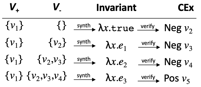
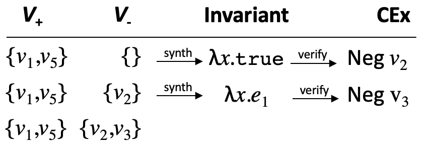
Figure 5. Partial traces of synthesis and verification results from a run of Hanoi without counterexample list caching enabled.

Consider the trace of Hanoi shown in Figure 5. In this example, Hanoi was just called with $v_{1}$ as the only positive example, and with no negative examples. With no negative examples, the synthesizer proposes ${\lambda x.\text{{\leavevmode\lstinline{{\lst@@@set@language\lst@@@set@numbers\lst@@@set@frame\lst@@@set@rulecolor\lst@@@set@numbers\lst@@@set@language\lst@@@set@language\linespread{0.9}{\@listingGroup{ltx_lst_keywords2}{\color[rgb]{0,0.3,0}true}}}}}}}$ as a candidate invariant and then verification subsequently provides the negative counterexample, $v_{2}$, which then becomes the only negative example in the next attempt at synthesis. This loop of proposing new invariants, and adding their negative counterexamples to the negative example set continues until $\lambda x.e_{3}$ is proposed, which provides the positive counterexample, $v_{5}$.

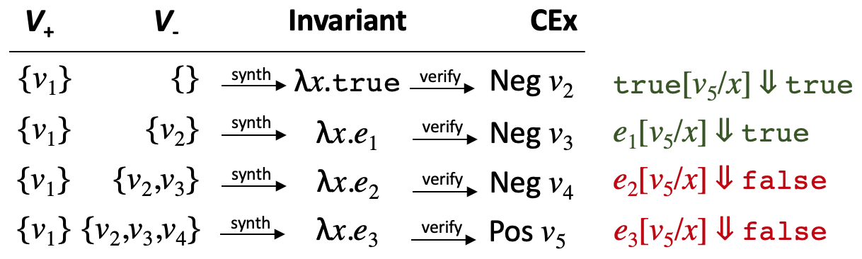
Figure 6. Results of running a positive counterexample on the trace shown in Figure 5.

Next, according to the unoptimized algorithm, one should begin a run with $\{v_{1},v_{5}\}$ as positive examples and no negative examples—see Figure 5 for a partial trace of this subsequent execution. Suppose that $v_{5}$ satisfies the first two synthesized invariants from the original run. In that case, those invariants will simply be synthesized again as the first two candidates of this new run, as shown in the figure. To avoid this recomputation, we cache these traces of synthesis and verification calls. When we receive a new positive example, we run it on the synthesized invariants in the trace, as shown in Figure 6. Because ${\lambda x.\text{{\leavevmode\lstinline{{\lst@@@set@language\lst@@@set@numbers\lst@@@set@frame\lst@@@set@rulecolor\lst@@@set@numbers\lst@@@set@language\lst@@@set@language\linespread{0.9}{\@listingGroup{ltx_lst_keywords2}{\color[rgb]{0,0.3,0}true}}}}}}}$ and $\lambda x.e_{1}$ both return true on $v_{5}$, we can skip the entirety of the trace shown in Figure 5 and begin by synthesizing from the testbed $V_{\mkern-2.0mu+}=\{v_{1},v_{5}\}$ and $V_{\mkern-2.0mu-}=\{v_{2},v_{3}\}$.

5. Experimental Results

We aim to answer the following research questions:

1. Can we infer sufficient representation invariants in practice?

2. What are the primary performance factors?

3. What effect on performance do our optimizations have?

4. How does our algorithm compare with prior work?

5.1. Benchmark Suite

We evaluate Hanoi on a total of 28 verification problems, most of which require reasoning over list or tree structures. We categorize them into the following four groups.

• VFA ($5$): Four modules from Verified Functional Algorithms (VFA) (Appel, 2018) that have interfaces and specifications over those interfaces, including tree- and list-based implementations of lookup tables and priority queues. We also experimented with a second version of priority queues that excludes the merge function.

• VFAExt ($3$): Three VFA modules with additional function(s) and corresponding specifications from the Coq (Team, 2019) standard library.

• Coq ($14$): Five tree- and list-based implementations of data structures from the Coq (Team, 2019) standard library. One additional problem for each of the five by introducing additional binary functions. Four more problems by extending interfaces with higher-order functions.

• Other ($6$): Six additional benchmarks of our own creation requiring reasoning over lists, natural numbers, monads and other basic data structures.

5.2. Experimental Setup

All experiments were performed on a 2.5 GHz Intel Core i7 processor with 16 GB of 1600 MHz DDR3 RAM running macOS Mojave. We ran each benchmark 10 times with a timeout of 30 minutes and report the average time. If any of the 10 runs time out then we consider the benchmark as a whole to have timed out.

5.3. Inferred Invariants

§​ 5.4 presents our results. Overall, Hanoi terminated with an invariant on 22 out of 28 benchmarks within the timeout bound. The second column shows the sizes of the inferred invariants, in terms of their abstract syntax trees.

Though our verifier is unsound, there was no effect on the reliability of the system on our benchmark suite: 22 of the 22 inferred invariants are correct. Further, some of them are quite sophisticated. For example, we synthesize a heap invariant, which requires that the the elements of each node’s subtrees is smaller than that node’s label. We synthesize invariants over lists including “max element first,” “no duplicates,” and “ordered.” If we allow the system to exceed the 30 min threshold, the system will infer a binary search tree invariant as well.

In seven of the cases above, we run into a limitation of the Myth synthesizer rather than our algorithm: Myth cannot synthesize functions that require recursive “helper” functions. To bypass this restriction, we added a true_maximum function (that finds the maximum element of a tree) to our tree-heap benchmark and a min_max_tree function (that finds the minimum and maximum elements of trees) to our bst and red-black-tree benchmarks. We added a * next to the names of benchmarks that we altered by providing a helper function in this way (see §​ 5.4).

5.4. Primary Performance Factors

Name	Size	Time (s)	TVT (s)	TVC	MVT (s)	TST (s)	TSC	MST (s)
[head to column names]generated-data-annotated.csv

Figure 7. Information from running Hanoi on our benchmark suite. Name is the name of the benchmark. Size is the size of the inferred invariant. Time is the time to run the benchmark from start to end. TVT is the total time spent verifying. TVC is the total number of verification calls. MVT is the average time for a single verification call. TST is the total time spent synthesizing. TSC is the total number of synthesis calls. MST is the average time for a single synthesis call. Benchmarks marked with a * were provided an additional function to enable synthesis by Myth.

When benchmarks complete within the 30 minute bound, most of the time is spent in verification. Indeed, for all but two of the terminating benchmarks, the total time spent synthesizing is under two seconds.

Three factors affect verification times significantly: (1) the strength of the specification, (2) the complexity of the underlying data structure, and (3) the presence of higher order functions. First, it takes our verifier longer to validate a true fact than to find a counterexample to a false one (validation requires enumeration of all tests; in contrast, the moment a counterexample is found, the enumeration is short-circuited). Many candidate invariants imply weak specifications but are not inductive. Hence weak specifications, ironically, are quite costly, because many candidate invariants wind up being sufficient (incurring a significant verification expense each time), only to be thrown away later when it turns out they are not inductive. Second, relatively simple data structures, like natural numbers and lists with numbers as their elements, take less time to verify than more complex data structures, like trees, tries, and lists with more complex elements. Third, like other complicated data types, the use of higher-order functions increases verification time. There are many ways to build a function, so enumeratively verifying a higher-order function requires searching through many possible functions.

However, the story is different for the complex benchmarks that do not complete within 30 minutes. When we ran Hanoi on our bst set benchmark, it completed in 78.4 minutes. Unlike the prior benchmarks, the majority of the time (65%) was spent in synthesis. Moreover, 30% of the total time was spent on the synthesis call that generated the final invariant. This indicates that Hanoi is currently not gated by the verifier, but by the synthesizer. Indeed, the implementation of bst set that includes binary functions like union and intersection is actually much faster than that without union and intersection, terminating within our 30 minute timeout. Adding these functions makes the verification harder, but Myth can use them to generate simpler invariants. Adding helper functions that permit simpler invariants also makes our implementation of a bst table verifiable in under 30 minutes.

Due to these limitations, we believe that a smarter synthesizer would be able to find more invariants. To this end, we built a prototype synthesizer that can generate more complex types of functions. This synthesizer has similarities to Myth as it is type-and-example directed and enumerative. However, where Myth can only synthesize simple recursive functions, this alternate synthesizer can synthesize folds, letting our synthesizer generate functions that require accumulators. Our synthesizer performs comparably to Myth, synthesizing invariants for the 20 benchmarks Myth that can solve an average of 11% slower. However, our synthesizer is also able to find the invariant for a binary heap (/vfa/tree-::-priqueue) without requiring helper functions or functions defined in the module in 185.4 seconds (55.8 seconds for /vfa/tree-::-priqueue+binfuncs), while Myth fails.

5.5. Comparisons

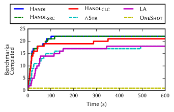
Figure 8. Number of benchmarks that terminate in a given time. Hanoi is the full Hanoi tool. Hanoi_-SRC is Hanoi with synthesis result caching turned off. Hanoi_-CLC is Hanoi with counterexample list caching turned off. $\wedge$Str is Hanoi using a conjunctive strengthening algorithm similar to that of LoopInvGen. LA is Hanoi using a counterexample generation strategy similar to that of LinearArbitrary. OneShot synthesizes based on the results of running the 30 smallest values on the specification. All the tests that terminated within the 30 minute timeout terminated within the first 10.

Figure 8 summarizes the results of running of Hanoi, Hanoi without optimizations, and our implementations of prior approaches adapted to our setting.

Impact of Optimizations.

The modes Hanoi_-SRC and Hanoi_-CLC tested the impacts of our optimizations described in §4.4. Hanoi_-SRC runs the benchmarks with synthesis result caching turned off. Hanoi_-CLC runs the benchmarks with counterexample list caching turned off.

Removing synthesis result caching does not have a large impact on the majority of benchmarks as the majority of our benchmarks spend relatively little time in synthesis. However, more complex benchmarks are able to enjoy the benefits of this optimization.

Counterexample list caching has significant impact on complex benchmarks as they have more synthesis and verification calls. The synthesizer requires more input/output examples to synthesize the correct invariant on complex benchmarks, so saving time reconstructing the negative examples via counterexample list caching has great impact.

Comparison to $\wedge$Str.

The $\wedge$Str mode simulates the LoopInvGen algorithm (Padhi et al., 2016), a related data-driven system for inferring loop invariants. When running $\wedge$Str, if a candidate invariant $\mathcal{I}_{1}$ is sufficient to prove the specification, but is not inductive, the algorithm attempts to synthesize a new predicate $\mathcal{I}_{2}$ such that ${v_{m}}\bm{:}{\tau_{m}}\mkern 8.0mu\leavevmode\resizebox{8.09995pt}{5.40005pt}{$\blacktriangleright$}^{\mathcal{I}_{1}\wedge\mathcal{I}_{2}}_{\mathcal{I}_{1}}\mkern 8.0mu\textnormal{{Valid}}$. In that case, $\mathcal{I}_{1}\wedge\mathcal{I}_{2}$ is considered the new candidate invariant. This process continues until either the conjoined invariants are inductive, or they are overly strong so a new positive counterexample is found, at which point the whole process restarts. Hanoi outperforms $\wedge$Str on all the benchmarks and solves 3 more benchmarks within 30 minutes. The main downside of $\wedge$Str is that it can only add new positive examples in order to weaken the candidate invariant after it has obviously over-strengthened. Hanoi, in contrast, uses visible inductiveness checks to eagerly weaken in a directed manner.

Comparison to LA.

LA mode simulates the LinearArbitrary algorithm (Zhu et al., 2018), which is used in a data-driven CHC solver. There are two differences from Hanoi. First, LA tries to satisfy individual inductiveness constraints, generated for each function in the module, one at a time rather than all at once. Second, rather than eagerly searching for visible inductiveness violations, only full inductiveness counterexamples are obtained. However, if a full inductiveness counterexample happens to also be a visible inductiveness counterexample then it is treated accordingly. Hanoi outperforms LA on all the benchmarks and is able to solve 4 more benchmarks within 30 minutes. While Hanoi checks eagerly for positive counterexamples, LA finds them nondeterministically. Without performing the guided search through visible inductiveness checks, the algorithm sometimes gets “stuck” in holes of negative counterexamples. While the algorithm does seem to emerge from these holes eventually, it takes time.

Comparison to OneShot.

The OneShot mode uses “one shot learning” rather than an interative CEGIS algorithm. The OneShot algorithm runs the specification over the smallest 30 elements of the concrete implementation type, tagging each element as either positive or negative. Doing so generates sets $V_{\mkern-2.0mu+}$ and $V_{\mkern-2.0mu-}$, which may be supplied to the synthesizer. Whatever invariant synthesized is returned as the result. (This algorithm only works when the specification quantifies over a single element of the abstract type, which is true for all but 7 of our benchmarks.) Running the OneShot algorithm fails on all but one of our benchmarks, coq/unique-list-set, and does so for a variety of reasons. On some benchmarks, Myth times out, indicating that the given synthesis problem was too hard, and Myth needed to be provided fewer examples to find the right invariant. On some benchmarks, Myth returns the wrong invariant, indicating that the synthesis problem was underspecified, and too few examples were given. Merely choosing some fixed number of examples to build the invariant with is insufficient, that fixed number is too high for some benchmarks, and too low for others.

6. Related Work

Inferring Representation Invariants.

To our knowledge, the only prior work that attempts to automatically infer representation invariants for data structures is the Deryaft system by Malik et al. (2007), which targets Java classes. There are three key differences between systems. First, Deryaft requires a fixed set of predicates (e.g., sortedness) as an input; the invariants generated are conjunctions of these predicates. In contrast, Hanoi can learn new predicates from a general grammar of programs. Second, the conjunction of predicates that Deryaft produces consists of those predicates that hold on a fixed set of examples (generated from test executions). There is no guarantee the final invariant is inductive. In contrast, Hanoi employs a CEGIS-based approach to refining the candidate invariant, terminating only when a sufficient representation invariant has been identified. Third, the Deryaft algorithm comes with no theoretical completeness guarantee.

Solving constrained Horn clauses.

Recently, several tools have been developed to infer predicates that satisfy a given set of constrained Horn clauses (CHCs). Inferring representation invariants can be seen as a special case of CHC solving, since all of our inductiveness constraints are Horn clauses (e.g., ${\left(\mathcal{I}_{\star}\mkern 6.0mus_{1}\right)\wedge\left(\mathcal{I}_{\star}\mkern 6.0mus_{2}\right)\mathrel{\leavevmode\resizebox{13.50002pt}{4.5pt}{$\implies$}}\left(\mathcal{I}_{\star}\mkern 6.0mu(\text{{\leavevmode\lstinline{{\lst@@@set@language\lst@@@set@numbers\lst@@@set@frame\lst@@@set@rulecolor\lst@@@set@numbers\lst@@@set@language\lst@@@set@language\linespread{0.9}{\@listingGroup{ltx_lst_identifier}{union}}}}}}}\ s_{1}\ s_{2})\right))$. CHCs can include multiple unknown predicates in their inference problem, whereas there is only one in ours.

However, existing CHC solvers do not support inference of recursive predicates, which is necessary to handle representation invariants over recursive data types. Several solvers support only arithmetic constraints (Fedyukovich et al., 2017; Zhu et al., 2018; Ezudheen et al., 2018), while others support arrays or bit vectors (Champion et al., 2018; Komuravelli et al., 2016; Hojjat and Rümmer, 2018) as well. To our knowledge, Eldarica (Hojjat and Rümmer, 2018) is the only CHC solver that supports algebraic data types. However, Eldarica only computes recursion-free solutions (Hojjat and Rümmer, 2018, Sec III C) and therefore cannot express the sortedness or no-duplicates properties, for instance.

Though they only handle arithmetic constraints, two of these solvers employ a data-driven technique that is similar to our approach, iterating between a synthesizer and a verifier (Zhu et al., 2018; Ezudheen et al., 2018). Like our work, the approach of Zhu et al. (2018) leverages the observation that handling inductiveness counterexamples $\left\langle x,y\right\rangle$ is easy when we know that $x$ is constructible. However, their approach simply checks if a counterexample to full inductiveness happens to have this property, while we exhaustively iterate through these counterexamples until a candidate invariant is visibly inductive. Intuitively, our approach minimizes the number of inductiveness counterexamples that must be treated heuristically. We show that this difference results in a significant performance improvement, and we have proven a completeness result for finite domains, while the approach of Zhu et al. (2018) lacks a completeness result. The approach of Ezudheen et al. (2018) does have a completeness result, and it applies to the infinite domain of integers. However, they achieve this guarantee through the use of a specialized synthesizer designed to handle inductiveness counterexamples directly, while our approach can use any off-the-shelf synthesizer. There is also no obvious analogue to our analysis of higher-order programs in this context.

Inferring inductive invariants.

There have been many techniques developed to infer individual inductive invariants for program verification, for example an inductive invariant for a loop or for a system transition relation. As discussed in §​ 2.2, module functions may consume or produce multiple arguments or results of the abstract type, which results in a more general class of inductiveness counterexamples, whereas loops and transition relations, when viewed as functions, consume and produce exactly one “state” (the analogue of an abstract value in our setting).

Hanoi is similar in structure to several data-driven invariant synthesis engines (Sharma and Aiken, 2016; Padhi et al., 2016; Ezudheen et al., 2018; Nguyen et al., 2017; Neider et al., 2018; Barbosa et al., 2019; Si et al., 2018; Le et al., 2019; Garg et al., 2016; Fedyukovich et al., 2017). We experimentally compared our algorithm to our implementations of the most closely related ones, adapted to the context of representation invariant synthesis (§​ 5.5). Broadly, the technical distinctions are similar to those described above for data-driven CHC solvers. In particular: (1) our development of visible inductiveness is novel; (2) aside from one tool (Garg et al., 2016) that depends upon a special-purpose synthesizer to handles inductiveness counterexamples directly, none are proven complete; (3) they cannot process higher-order programs; and (4) to our knowledge, none infer recursive invariants.

The ic3 algorithm for SAT-based model checking employs a notion of relative inductiveness (Bradley, [n.d.]), which is closely related to our notions of conditional and visible inductiveness. Formally, relative inductiveness is the special case of our conditional inductiveness relation ${v}\bm{:}{\tau}\mkern 8.0mu\leavevmode\resizebox{8.09995pt}{5.40005pt}{$\blacktriangleright$}^{P}_{Q}\mkern 8.0mu\textnormal{{Valid}}$ where $P$ has the form $Q^{\prime}\wedge Q$ and $\tau=\alpha\rightarrow\alpha$. The ic3 algorithm uses relative inductiveness to incrementally produce an inductive invariant, by iteratively identifying a state $s$ that leads to a property violation and then conjoining an inductive strengthening of $\neg s$ to the candidate invariant. Our notion of visible inductiveness is also used to incrementally produce an inductive invariant, but it works in the opposite direction: we iteratively identify constructible values of the abstract type and use them to weaken the candidate invariant. This approach is a natural fit for our data-driven setting.

Automatic data structure verification.

The Leon framework (Suter et al., 2011) can automatically verify correctness of data structure implementations, but to do so, a user must manually define an abstraction function, which plays a similar role to a representation invariant. Namely, the abstraction function is a partial function mapping an element of the concrete type to an element of the abstract type.

There are many techniques for proving properties of heap-based data structures, including shape analysis (Sagiv et al., 1999) and liquid types (Kawaguchi et al., 2009). These techniques can prove and/or infer sophisticated invariants, often of imperative code. However, they are designed to tackle a different problem and do not infer the inductive representation invariants that are needed to prove modules correct.

7. Conclusion

We present a novel algorithm for synthesis of representation invariants. Our key insight is that it is possible to drive progress of the algorithm towards its goal not by eagerly searching for fully inductive invariants, but rather by searching first for visibly inductive invariants. We have proven that our algorthm is sound and complete, given a sound and complete verifier and synthesizer, for a first-order type theory with finite types. We also explain how to extend the algorithm to modules containing higher-order functions, which involves using contracts to validate and collect objects that cross the module boundary. We evaluate our algorithm on 28 benchmarks and find that we are able to synthesize 22 of the invariants within 30 minutes (and most of those in under a minute). Our algorithm is defined independently of the black-box verifier and synthesizers; as research in verifier and synthesizer technologies improve, so too will the capabilities of our overall system. While the tool is currently fully automated, we view this as a step towards an interactive approach to helping users of proof assistants produce correct representation invariants.

Appendix A Full Example List

Figure 9. Information from running Hanoi on our benchmark suite. Name is the name of the benchmark. Size is the size of the inferred invariant. Time is the time to run the benchmark from start to end. TVT is the total time spent verifying. TVC is the total number of verification calls. MVT is the average time for a single verification call. TST is the total time spent synthesizing. TSC is the total number of synthesis calls. MST is the average time for a single synthesis call. Benchmarks marked with a * were provided an additional function to enable synthesis by Myth. Elided benchmarks are marked in bold.

See Figure 5.4.

Appendix B Proofs of Theorems

B.1. Additional Definitions

For convenience, we lift the notion of constructibility to sets and predicates:

Definition B.1 ($\tau$-Constructible Set: $\bm{\mathfrak{C}}_{\mkern 1.0mu\mathbf{M}}\left[S\mkern 3.0mu\bm{;}\tau\right]$).

A set $S$ of values is said to be $\tau$-constructible using $\mathbf{M}$, denoted $\bm{\mathfrak{C}}_{\mkern 1.0mu\mathbf{M}}\left[S\mkern 3.0mu\bm{;}\tau\right]$, iff every element of $S$ is $\tau$-constructible using $\mathbf{M}$, i.e. $\forall\mkern 2.0muv\in S\mkern 2.0mu\ldotp\bm{\mathfrak{C}}_{\mkern 1.0mu\mathbf{M}}\left[v\mkern 3.0mu\bm{;}\tau\right]$.

Definition B.2 ($\tau$-Constructible Predicate: $\bm{\mathfrak{C}}_{\mkern 1.0mu\mathbf{M}}\left[p\mkern 3.0mu\bm{;}\tau\right]$).

A predicate $p\bm{:}\left(\tau[\alpha\mapsto\tau_{c}]\to\textnormal{{bool}}\right)$ is said to be $\tau$-constructible using $\mathbf{M}$, denoted $\bm{\mathfrak{C}}_{\mkern 1.0mu\mathbf{M}}\left[p\mkern 3.0mu\bm{;}\tau\right]$, iff the set of values that satisfy $p$ is $\tau$-constructible using $\mathbf{M}$, i.e. $\bm{\mathfrak{C}}_{\mkern 1.0mu\mathbf{M}}\left[\{v\mid p\ v\}\mkern 3.0mu\bm{;}\tau\right]$.

We omit $\mathbf{M}$ from the subscript when it is clear from context.

B.2. Type Safety of Conditional Inductiveness Rules

Lemma B.3.

If  ${v}\bm{:}{\tau}\mkern 8.0mu\leavevmode\resizebox{8.09995pt}{5.40005pt}{$\blacktriangleright$}^{P}_{Q}\mkern 8.0mu\textnormal{{Valid}}$ then  $\vdash v\bm{:}\tau[\alpha\mapsto\tau_{c}]$.

Proof.

We prove this using induction on the derivation of ${v}\bm{:}{\tau}\mkern 8.0mu\leavevmode\resizebox{8.09995pt}{5.40005pt}{$\blacktriangleright$}^{P}_{Q}\mkern 8.0mu\textnormal{{Valid}}$. Consider the last rule applied.

• LABEL:rule:i-base-valid:

Trivial since we have that $v=w$, $\tau=\beta$ and $\vdash w\bm{:}\beta$. • LABEL:rule:i-abs-valid: Trivial since we have that $\tau=\alpha$ and $\vdash v\bm{:}\tau_{c}$. • LABEL:rule:i-prod-valid: We have that (a) $v=\left\langle v_{1},v_{2}\right\rangle$, (b) $\tau=\left(\tau_{1}\ast\,\tau_{2}\right)$ (c) ${v_{1}}\bm{:}{\tau_{1}}\mkern 8.0mu\leavevmode\resizebox{8.09995pt}{5.40005pt}{$\blacktriangleright$}^{P}_{Q}\mkern 8.0mu\textnormal{{Valid}}$, and (d) ${v_{2}}\bm{:}{\tau_{2}}\mkern 8.0mu\leavevmode\resizebox{8.09995pt}{5.40005pt}{$\blacktriangleright$}^{P}_{Q}\mkern 8.0mu\textnormal{{Valid}}$. Then, $\vdash v_{1}\bm{:}\tau_{1}[\alpha\mapsto\tau_{c}]$ and $\vdash v_{2}\bm{:}\tau_{2}[\alpha\mapsto\tau_{c}]$ by induction. Hence, $\vdash\left\langle v_{1},v_{2}\right\rangle\bm{:}\left(\tau_{1}\ast\,\tau_{2}\right)[\alpha\mapsto\tau_{c}]$ and the claim follows. • LABEL:rule:i-fun-valid: Trivial since we have that $\vdash v\bm{:}\left(\sigma_{1}\to\tau_{2}\right)[\alpha\mapsto\tau_{c}]$ and $\tau=\left(\sigma_{1}\to\tau_{2}\right)$. ∎

Lemma B.4.

If ${v}\bm{:}{\tau}\mkern 8.0mu\leavevmode\resizebox{8.09995pt}{5.40005pt}{$\blacktriangleright$}^{P}_{Q}\mkern 8.0mu\textnormal{{C\kern 0.75ptEx}}\,\left\langle S,V\right\rangle$ then $\vdash v\bm{:}\tau[\alpha\mapsto\tau_{c}]$.

Proof.

We prove this using induction on the derivation of ${v}\bm{:}{\tau}\mkern 8.0mu\leavevmode\resizebox{8.09995pt}{5.40005pt}{$\blacktriangleright$}^{P}_{Q}\mkern 8.0mu\textnormal{{C\kern 0.75ptEx}}\,\left\langle S,V\right\rangle$. Consider the last rule applied.

• LABEL:rule:i-abs-cex:

Trivial since we have that $\tau=\alpha$ and $\{\}\vdash v\bm{:}\tau_{c}$. • LABEL:rule:i-prod-cex-1: We have that (a) $v=\left\langle v_{1},v_{2}\right\rangle$, (b) $\tau=\left(\tau_{1}\ast\,\tau_{2}\right)$ (c) ${v_{1}}\bm{:}{\tau_{1}}\mkern 8.0mu\leavevmode\resizebox{8.09995pt}{5.40005pt}{$\blacktriangleright$}^{P}_{Q}\mkern 8.0mu\textnormal{{C\kern 0.75ptEx}}\,\left\langle S,V\right\rangle$, and (d) $\vdash v_{2}\bm{:}\tau_{2}[\alpha\mapsto\tau_{c}]$. Then, $\vdash v_{1}\bm{:}\tau_{1}[\alpha\mapsto\tau_{c}]$ by induction. Hence, $\vdash\left\langle v_{1},v_{2}\right\rangle\bm{:}\left(\tau_{1}\ast\,\tau_{2}\right)[\alpha\mapsto\tau_{c}]$ and the claim follows. • LABEL:rule:i-prod-cex-2: Similar to LABEL:rule:i-prod-cex-1 above. • LABEL:rule:i-fun-cex: Trivial since we have that $\vdash v\bm{:}\left(\sigma_{1}\to\tau_{2}\right)[\alpha\mapsto\tau_{c}]$ and $\tau=\left(\sigma_{1}\to\tau_{2}\right)$. ∎

B.3. Soundness of Hanoi

Lemma B.5.

If  Verify is sound, then $\left(\textnormal{{NoNegatives}}\mkern 6.0mu\mathcal{I}\right)$= Valid $\implies$ $\mathbf{M}\bm{:}\mathbf{F}\models_{\raisebox{-0.78749pt}{$\mathcal{I}$}}\varphi$

Proof.

We explicitly check for sufficiency at LABEL:line:sufficiency-check, and for inductiveness at LABEL:line:inductiveness-check. NoNegatives returns Valid only if both these checks succeed. Since Verify is assumed to be sound, the claim immediately follows. ∎

Theorem 3.9.

If  Verify is sound, then Hanoi is sound.

Proof.

Since Hanoi returns an invariant $\mathcal{I}$ only at LABEL:line:repinvgen-result, when $\left(\textnormal{{NoNegatives}}\mkern 6.0mu\mathcal{I}\right)=\textnormal{{Valid}}$, the claim immediately follows from Lemma B.5. ∎

B.4. Completeness of Hanoi

Lemma B.6.

$\bm{\mathfrak{C}}_{\mkern 1.0mu}\left[Q\mkern 3.0mu\bm{;}\alpha\right]\wedge{v}\bm{:}{\sigma}\mkern 8.0mu\leavevmode\resizebox{8.09995pt}{5.40005pt}{$\blacktriangleright$}^{P}_{Q}\mkern 8.0mu\textnormal{{Valid}}\mathrel{\leavevmode\resizebox{13.50002pt}{4.5pt}{$\implies$}}\bm{\mathfrak{C}}_{\mkern 1.0mu}\left[v\mkern 3.0mu\bm{;}\sigma\right]$.

Proof.

We prove this using induction on the derivation of ${v}\bm{:}{\sigma}\mkern 8.0mu\leavevmode\resizebox{8.09995pt}{5.40005pt}{$\blacktriangleright$}^{P}_{Q}\mkern 8.0mu\textnormal{{Valid}}$. Consider the last rule applied.

• LABEL:rule:i-base-valid:

Trivial since values of type $\beta$ are always Constructible. • LABEL:rule:i-abs-valid: Then $\sigma=\alpha$ and $\left(Q\mkern 6.0muv\right)$. Then since $\bm{\mathfrak{C}}_{\mkern 1.0mu}\left[Q\mkern 3.0mu\bm{;}\alpha\right]$, the claim follows immediately from Definition B.2. • LABEL:rule:i-prod-valid: We have that (a) $\sigma=\left(\sigma_{1}\ast\,\sigma_{2}\right)$, (b) $v=\left\langle v_{1},v_{2}\right\rangle$, (c) ${v_{1}}\bm{:}{\sigma_{1}}\mkern 8.0mu\leavevmode\resizebox{8.09995pt}{5.40005pt}{$\blacktriangleright$}^{P}_{Q}\mkern 8.0mu\textnormal{{Valid}}$, and (d) ${v_{2}}\bm{:}{\sigma_{2}}\mkern 8.0mu\leavevmode\resizebox{8.09995pt}{5.40005pt}{$\blacktriangleright$}^{P}_{Q}\mkern 8.0mu\textnormal{{Valid}}$. Then by induction we have that $\bm{\mathfrak{C}}_{\mkern 1.0mu}\left[v_{1}\mkern 3.0mu\bm{;}\sigma_{1}\right]$ and $\bm{\mathfrak{C}}_{\mkern 1.0mu}\left[v_{2}\mkern 3.0mu\bm{;}\sigma_{2}\right]$, hence also $\bm{\mathfrak{C}}_{\mkern 1.0mu}\left[v\mkern 3.0mu\bm{;}\sigma\right]$. ∎

Lemma B.7.

${v}\bm{:}{\sigma}\mkern 8.0mu\leavevmode\resizebox{8.09995pt}{5.40005pt}{$\blacktriangleright$}^{P}_{Q}\mkern 8.0mu\textnormal{{Valid}}\ \mathrel{\leavevmode\resizebox{13.50002pt}{4.5pt}{$\implies$}}\ \forall\mkern 2.0mux\in\left\{\mkern-3.875mu\middle|\,v\,\middle|\mkern-3.875mu\right\}_{\sigma}\mkern 2.0mu\ldotp\left(Q\mkern 6.0mux\right)$.

Proof.

We prove this using induction on the derivation of ${v}\bm{:}{\sigma}\mkern 8.0mu\leavevmode\resizebox{8.09995pt}{5.40005pt}{$\blacktriangleright$}^{P}_{Q}\mkern 8.0mu\textnormal{{Valid}}$. Consider the last rule applied.

• LABEL:rule:i-base-valid:

Trivial since $\left\{\mkern-3.875mu\middle|\,w\,\middle|\mkern-3.875mu\right\}_{\beta}=\emptyset$. • LABEL:rule:i-abs-valid: We have $\vdash v\bm{:}\tau_{c}$ and $\left(Q\mkern 6.0muv\right)$. Since $\sigma=\alpha$, due to LABEL:rule:c-abs we also have $\left\{\mkern-3.875mu\middle|\,v\,\middle|\mkern-3.875mu\right\}_{\alpha}=\{v\}$. Then the claim follows. • LABEL:rule:i-prod-valid: We have that (a) $\sigma=\left(\sigma_{1}\ast\,\sigma_{2}\right)$, (b) $v=\left\langle v_{1},v_{2}\right\rangle$, (c) ${v_{1}}\bm{:}{\sigma_{1}}\mkern 8.0mu\leavevmode\resizebox{8.09995pt}{5.40005pt}{$\blacktriangleright$}^{P}_{Q}\mkern 8.0mu\textnormal{{Valid}}$, and (d) ${v_{2}}\bm{:}{\sigma_{2}}\mkern 8.0mu\leavevmode\resizebox{8.09995pt}{5.40005pt}{$\blacktriangleright$}^{P}_{Q}\mkern 8.0mu\textnormal{{Valid}}$. Since $\left\{\mkern-3.875mu\middle|\,\left\langle v_{1},v_{2}\right\rangle\,\middle|\mkern-3.875mu\right\}_{\left(\sigma_{1}\ast\,\sigma_{2}\right)}=\left\{\mkern-3.875mu\middle|\,v_{1}\,\middle|\mkern-3.875mu\right\}_{\sigma_{1}}\cup\left\{\mkern-3.875mu\middle|\,v_{2}\,\middle|\mkern-3.875mu\right\}_{\sigma_{2}}$ by LABEL:rule:c-prod, the claim follows by induction. ∎

Lemma B.8.

$\forall\mkern 2.0mux\in\left\{\mkern-3.875mu\middle|\,v\,\middle|\mkern-3.875mu\right\}_{\sigma}\mkern 2.0mu\ldotp\left(Q\mkern 6.0mux\right)\mathrel{\leavevmode\resizebox{13.50002pt}{4.5pt}{$\implies$}}{v}\bm{:}{\sigma}\mkern 8.0mu\leavevmode\resizebox{8.09995pt}{5.40005pt}{$\blacktriangleright$}^{P}_{Q}\mkern 8.0mu\textnormal{{Valid}}$.

Proof.

We prove this using induction on the derivation of $\left\{\mkern-3.875mu\middle|\,v\,\middle|\mkern-3.875mu\right\}_{\sigma}$. Consider the last rule applied:

• LABEL:rule:c-base:

Trivial since $\left\{\mkern-3.875mu\middle|\,w\,\middle|\mkern-3.875mu\right\}_{\beta}=\emptyset$. • LABEL:rule:c-abs: We have that (a) $\sigma=\alpha$, (b) $\vdash v\bm{:}\tau_{c}$, and (c) $\left\{\mkern-3.875mu\middle|\,v\,\middle|\mkern-3.875mu\right\}_{\alpha}=\{v\}$. We also have $\left(Q\mkern 6.0muv\right)$ by assumption. Then, we have that ${v}\bm{:}{\alpha}\mkern 8.0mu\leavevmode\resizebox{8.09995pt}{5.40005pt}{$\blacktriangleright$}^{P}_{Q}\mkern 8.0mu\textnormal{{Valid}}$ by LABEL:rule:i-abs-valid. • LABEL:rule:c-prod: We have that $\left\{\mkern-3.875mu\middle|\,\left\langle v_{1},v_{2}\right\rangle\,\middle|\mkern-3.875mu\right\}_{\left(\sigma_{1}\ast\,\sigma_{2}\right)}=\left\{\mkern-3.875mu\middle|\,v_{1}\,\middle|\mkern-3.875mu\right\}_{\sigma_{1}}\cup\left\{\mkern-3.875mu\middle|\,v_{2}\,\middle|\mkern-3.875mu\right\}_{\sigma_{2}}$. Also, since $\forall\mkern 2.0mux\in\left\{\mkern-3.875mu\middle|\,v_{1}\,\middle|\mkern-3.875mu\right\}_{\sigma_{1}}\cup\left\{\mkern-3.875mu\middle|\,v_{2}\,\middle|\mkern-3.875mu\right\}_{\sigma_{2}}\mkern 2.0mu\ldotp\left(Q\mkern 6.0mux\right)$ by assumption, we have that ${v_{1}}\bm{:}{\sigma_{1}}\mkern 8.0mu\leavevmode\resizebox{8.09995pt}{5.40005pt}{$\blacktriangleright$}^{P}_{Q}\mkern 8.0mu\textnormal{{Valid}}$ and ${v_{2}}\bm{:}{\sigma_{2}}\mkern 8.0mu\leavevmode\resizebox{8.09995pt}{5.40005pt}{$\blacktriangleright$}^{P}_{Q}\mkern 8.0mu\textnormal{{Valid}}$ by induction. Then, ${\left\langle v_{1},v_{2}\right\rangle}\bm{:}{\left(\sigma_{1}\ast\,\sigma_{2}\right)}\mkern 8.0mu\leavevmode\resizebox{8.09995pt}{5.40005pt}{$\blacktriangleright$}^{P}_{Q}\mkern 8.0mu\textnormal{{Valid}}$ follows by LABEL:rule:i-prod-valid. ∎

Lemma B.9.

If ${v}\bm{:}{\tau}\mkern 8.0mu\leavevmode\resizebox{8.09995pt}{5.40005pt}{$\blacktriangleright$}^{P}_{Q}\mkern 8.0mu\textnormal{{C\kern 0.75ptEx}}\,\left\langle S,V\right\rangle$, then (1) $\forall\mkern 2.0mux\in S\mkern 2.0mu\ldotp\left(P\mkern 6.0mux\right)$, (2) $V\neq\emptyset$, and (3) $\forall\mkern 2.0mux\in V\mkern 2.0mu\ldotp\neg\left(Q\mkern 6.0mux\right)$.

Proof.

We prove this using induction on the derivation of ${v}\bm{:}{\tau}\mkern 8.0mu\leavevmode\resizebox{8.09995pt}{5.40005pt}{$\blacktriangleright$}^{P}_{Q}\mkern 8.0mu\textnormal{{C\kern 0.75ptEx}}\,\left\langle S,V\right\rangle$. Consider the last rule applied.

• LABEL:rule:i-abs-cex:

Straightforward since $S=\emptyset$, $V=\{v\}$. • LABEL:rule:i-prod-cex-1 and LABEL:rule:i-prod-cex-2: Follow immediately from the induction hypothesis. • LABEL:rule:i-fun-cex: We have that (a) ${v_{1}}\bm{:}{\sigma_{1}}\mkern 8.0mu\leavevmode\resizebox{8.09995pt}{5.40005pt}{$\blacktriangleright$}^{Q}_{P}\mkern 8.0mu\textnormal{{Valid}}$, and (b) ${v_{2}}\bm{:}{\tau_{2}}\mkern 8.0mu\leavevmode\resizebox{8.09995pt}{5.40005pt}{$\blacktriangleright$}^{P}_{Q}\mkern 8.0mu\textnormal{{C\kern 0.75ptEx}}\,\left\langle S^{\prime},V\right\rangle$. Then, (2) and (3) are satisfied by the induction hypothesis. Due to Lemma B.7, we have that $\forall\mkern 2.0mux\in\left\{\mkern-3.875mu\middle|\,v_{1}\,\middle|\mkern-3.875mu\right\}_{\sigma_{1}}\mkern 2.0mu\ldotp\left(P\mkern 6.0mux\right)$. Then, since $\forall\mkern 2.0mux\in S^{\prime}\mkern 2.0mu\ldotp\left(P\mkern 6.0mux\right)$ from the induction hypothesis, we have that $\forall\mkern 2.0mux\in\left\{\mkern-3.875mu\middle|\,v_{1}\,\middle|\mkern-3.875mu\right\}_{\sigma_{1}}\cup S^{\prime}\mkern 2.0mu\ldotp\left(P\mkern 6.0mux\right)$. Hence, (1) is satisfied as well since $S=\left\{\mkern-3.875mu\middle|\,v_{1}\,\middle|\mkern-3.875mu\right\}_{\sigma_{1}}\cup S^{\prime}$. ∎

Lemma B.10.

If $\bm{\mathfrak{C}}_{\mkern 1.0mu}\left[v\mkern 3.0mu\bm{;}\tau\right]\wedge\bm{\mathfrak{C}}_{\mkern 1.0mu}\left[P\mkern 3.0mu\bm{;}\alpha\right]\wedge{v}\bm{:}{\tau}\mkern 8.0mu\leavevmode\resizebox{8.09995pt}{5.40005pt}{$\blacktriangleright$}^{P}_{Q}\mkern 8.0mu\textnormal{{C\kern 0.75ptEx}}\,\left\langle S,V\right\rangle$ then $\bm{\mathfrak{C}}_{\mkern 1.0mu}\left[V\mkern 3.0mu\bm{;}\alpha\right]$.

Proof.

We prove this using induction on the derivation of ${v}\bm{:}{\tau}\mkern 8.0mu\leavevmode\resizebox{8.09995pt}{5.40005pt}{$\blacktriangleright$}^{P}_{Q}\mkern 8.0mu\textnormal{{C\kern 0.75ptEx}}\,\left\langle S,V\right\rangle$. Consider the last rule applied.

• LABEL:rule:i-abs-cex:

Straightforward since we have $\alpha=\tau$ and $\bm{\mathfrak{C}}_{\mkern 1.0mu\mathbf{M}}\left[v\mkern 3.0mu\bm{;}\tau\right]$ holds by assumption. • LABEL:rule:i-prod-cex-1: We have ${v_{1}}\bm{:}{\tau_{1}}\mkern 8.0mu\leavevmode\resizebox{8.09995pt}{5.40005pt}{$\blacktriangleright$}^{P}_{Q}\mkern 8.0mu\textnormal{{C\kern 0.75ptEx}}\,\left\langle S,V\right\rangle$, and it is easy to show that $\bm{\mathfrak{C}}_{\mkern 1.0mu}\left[\left\langle v_{1},v_{2}\right\rangle\mkern 3.0mu\bm{;}\left(\tau_{1}\ast\,\tau_{2}\right)\right]\mathrel{\leavevmode\resizebox{13.50002pt}{4.5pt}{$\implies$}}\bm{\mathfrak{C}}_{\mkern 1.0mu}\left[v_{1}\mkern 3.0mu\bm{;}\tau_{1}\right]$. Then the claim follows by induction. • LABEL:rule:i-prod-cex-2: Similar to LABEL:rule:i-prod-cex-1 above. • LABEL:rule:i-fun-cex: We have that (a) ${v_{1}}\bm{:}{\sigma_{1}}\mkern 8.0mu\leavevmode\resizebox{8.09995pt}{5.40005pt}{$\blacktriangleright$}^{Q}_{P}\mkern 8.0mu\textnormal{{Valid}}$, and (b) ${v_{2}}\bm{:}{\tau_{2}}\mkern 8.0mu\leavevmode\resizebox{8.09995pt}{5.40005pt}{$\blacktriangleright$}^{P}_{Q}\mkern 8.0mu\textnormal{{C\kern 0.75ptEx}}\,\left\langle S^{\prime},V\right\rangle$. Due to Lemma B.6, we also have that $\bm{\mathfrak{C}}_{\mkern 1.0mu}\left[v_{1}\mkern 3.0mu\bm{;}\sigma_{1}\right]$. Hence $\bm{\mathfrak{C}}_{\mkern 1.0mu}\left[v_{2}\mkern 3.0mu\bm{;}\tau_{2}\right]$ since $\left(v\mkern 6.0muv_{1}\right)\Downarrow v_{2}$, and then the claim follows by induction. ∎

Lemma B.11.

If ${v}\bm{:}{\tau}\mkern 8.0mu\leavevmode\resizebox{8.09995pt}{5.40005pt}{$\blacktriangleright$}^{P}_{Q}\mkern 8.0mu\textnormal{{Valid}}\wedge{v}\bm{:}{\tau}\mkern 8.0mu\leavevmode\resizebox{8.09995pt}{5.40005pt}{$\blacktriangleright$}^{Q}_{Q}\mkern 8.0mu\textnormal{{C\kern 0.75ptEx}}\,\left\langle S,V\right\rangle$, then $\exists\mkern 2.0mux\in S\mkern 2.0mu\ldotp\neg\left(P\mkern 6.0mux\right)$.

Proof.

We prove this using induction on the derivation of ${v}\bm{:}{\tau}\mkern 8.0mu\leavevmode\resizebox{8.09995pt}{5.40005pt}{$\blacktriangleright$}^{Q}_{Q}\mkern 8.0mu\textnormal{{C\kern 0.75ptEx}}\,\left\langle S,V\right\rangle$. Consider the last rule applied.

• LABEL:rule:i-abs-cex:

Impossible, since ${v}\bm{:}{\tau}\mkern 8.0mu\leavevmode\resizebox{8.09995pt}{5.40005pt}{$\blacktriangleright$}^{P}_{Q}\mkern 8.0mu\textnormal{{Valid}}\mathrel{\leavevmode\resizebox{13.50002pt}{4.5pt}{$\implies$}}\left(Q\mkern 6.0muv\right)$. • LABEL:rule:i-prod-cex-1: We have ${v_{1}}\bm{:}{\tau_{1}}\mkern 8.0mu\leavevmode\resizebox{8.09995pt}{5.40005pt}{$\blacktriangleright$}^{Q}_{Q}\mkern 8.0mu\textnormal{{C\kern 0.75ptEx}}\,\left\langle S,V\right\rangle$. Due to the assumption ${\left\langle v_{1},v_{2}\right\rangle}\bm{:}{\left(\tau_{1}\ast\,\tau_{2}\right)}\mkern 8.0mu\leavevmode\resizebox{8.09995pt}{5.40005pt}{$\blacktriangleright$}^{P}_{Q}\mkern 8.0mu\textnormal{{Valid}}$, and LABEL:rule:i-prod-valid, we also have ${v_{1}}\bm{:}{\tau_{1}}\mkern 8.0mu\leavevmode\resizebox{8.09995pt}{5.40005pt}{$\blacktriangleright$}^{P}_{Q}\mkern 8.0mu\textnormal{{Valid}}$. Then, the claim follows immediately from the induction hypothesis. • LABEL:rule:i-prod-cex-2: Similar to LABEL:rule:i-prod-cex-1 above. • LABEL:rule:i-fun-cex: We have that (a) ${v_{1}}\bm{:}{\sigma_{1}}\mkern 8.0mu\leavevmode\resizebox{8.09995pt}{5.40005pt}{$\blacktriangleright$}^{Q}_{Q}\mkern 8.0mu\textnormal{{Valid}}$, and (b) ${v_{2}}\bm{:}{\tau_{2}}\mkern 8.0mu\leavevmode\resizebox{8.09995pt}{5.40005pt}{$\blacktriangleright$}^{Q}_{Q}\mkern 8.0mu\textnormal{{C\kern 0.75ptEx}}\,\left\langle S^{\prime},V\right\rangle$. Since ${v}\bm{:}{\tau}\mkern 8.0mu\leavevmode\resizebox{8.09995pt}{5.40005pt}{$\blacktriangleright$}^{P}_{Q}\mkern 8.0mu\textnormal{{Valid}}$, we have two possibilities: – ${v_{1}}\bm{:}{\sigma_{1}}\mkern 8.0mu\leavevmode\resizebox{8.09995pt}{5.40005pt}{$\blacktriangleright$}^{Q}_{P}\mkern 8.0mu\textnormal{{Valid}}$: We have ${v_{2}}\bm{:}{\tau_{2}}\mkern 8.0mu\leavevmode\resizebox{8.09995pt}{5.40005pt}{$\blacktriangleright$}^{P}_{Q}\mkern 8.0mu\textnormal{{Valid}}$. Then, due to (b) above, we have $\exists\mkern 2.0mux\in S^{\prime}\mkern 2.0mu\ldotp\neg\left(P\mkern 6.0mux\right)$ by induction. – $\neg({v_{1}}\bm{:}{\sigma_{1}}\mkern 8.0mu\leavevmode\resizebox{8.09995pt}{5.40005pt}{$\blacktriangleright$}^{Q}_{P}\mkern 8.0mu\textnormal{{Valid}})$: Due to (the contrapositive of) Lemma B.8, we have that $\exists\mkern 2.0mux\in\left\{\mkern-3.875mu\middle|\,v_{1}\,\middle|\mkern-3.875mu\right\}_{\sigma_{1}}\mkern 2.0mu\ldotp\neg\left(P\mkern 6.0mux\right)$. The claim follows since $S=S^{\prime}\cup\left\{\mkern-3.875mu\middle|\,v_{1}\,\middle|\mkern-3.875mu\right\}_{\sigma_{1}}$. ∎

Lemma B.12.

If  Verify is sound and complete, and $V_{\mkern-2.0mu+}$ and $\mathcal{I}$ satisfy $\bm{\mathfrak{C}}_{\mkern 1.0mu}\left[V_{\mkern-2.0mu+}\mkern 3.0mu\bm{;}\alpha\right]\wedge\forall\mkern 2.0muv\in V_{\mkern-2.0mu+}\mkern 2.0mu\ldotp\left(\mathcal{I}\mkern 6.0muv\right)$, then

$\mathrel{\leavevmode\resizebox{13.50002pt}{4.5pt}{$\implies$}}V\neq\emptyset\ \wedge\ \bm{\mathfrak{C}}_{\mkern 1.0mu}\left[V\mkern 3.0mu\bm{;}\alpha\right]\ \wedge\ \left(\forall\mkern 2.0muv\in V\mkern 2.0mu\ldotp\neg\left(\mathcal{I}\mkern 6.0muv\right)\wedge v\not\in V_{\mkern-2.0mu+}\right)$ (2) $\left(\textnormal{{ClosedPositives}}\mkern 6.0muV_{\mkern-2.0mu+}\mkern 6.0mu\mathcal{I}\right)=\textnormal{{Valid}}$ $\mathrel{\leavevmode\resizebox{13.50002pt}{4.5pt}{$\implies$}}{v_{m}}\bm{:}{\tau_{m}}\mkern 8.0mu\leavevmode\resizebox{8.09995pt}{5.40005pt}{$\blacktriangleright$}^{V_{\mkern-2.0mu+}}_{\mathcal{I}}\mkern 8.0mu\textnormal{{Valid}}$

Proof.

On expanding CondInductive, (2) immediately follows. For (1), we first observe that $v_{m}$ is trivially constructible, and thus $\bm{\mathfrak{C}}_{\mkern 1.0mu}\left[V\mkern 3.0mu\bm{;}\alpha\right]$ by Lemma B.10. Due to Lemma B.9, we also have that $V\neq\emptyset\wedge\forall\mkern 2.0mux\in V\mkern 2.0mu\ldotp\neg\left(\mathcal{I}\mkern 6.0mux\right)$. Finally, we have that $\forall\mkern 2.0mux\in V\mkern 2.0mu\ldotp v\not\in V_{\mkern-2.0mu+}$ since $\forall\mkern 2.0muv\in V_{\mkern-2.0mu+}\mkern 2.0mu\ldotp\left(\mathcal{I}\mkern 6.0muv\right)$ by assumption. ∎

Lemma B.13.

If  Verify is sound and complete, then

$\mathrel{\leavevmode\resizebox{13.50002pt}{4.5pt}{$\implies$}}\left(S\neq\emptyset\ \ \wedge\ \ \forall\mkern 2.0muv\in S\mkern 2.0mu\ldotp\left(\mathcal{I}\mkern 6.0muv\right)\wedge\neg\left(\varphi\mkern 6.0muv\right)\right)$   $\vee\mkern 12.0mu\left(\forall\mkern 2.0muv\in S\mkern 2.0mu\ldotp\left(\mathcal{I}\mkern 6.0muv\right)\ \ \wedge\ \ \exists\mkern 2.0muV\mkern 2.0mu\ldotp{v_{m}}\bm{:}{\tau_{m}}\mkern 8.0mu\leavevmode\resizebox{8.09995pt}{5.40005pt}{$\blacktriangleright$}^{\mathcal{I}}_{\mathcal{I}}\mkern 8.0mu\textnormal{{C\kern 0.75ptEx}}\,\left\langle S,V\right\rangle\right)$ (2) $\left(\textnormal{{NoNegatives}}\mkern 6.0mu\mathcal{I}\right)=\textnormal{{Valid}}$ $\mathrel{\leavevmode\resizebox{13.50002pt}{4.5pt}{$\implies$}}{v_{m}}\bm{:}{\tau_{m}}\mkern 8.0mu\leavevmode\resizebox{8.09995pt}{5.40005pt}{$\blacktriangleright$}^{\mathcal{I}}_{\mathcal{I}}\mkern 8.0mu\textnormal{{Valid}}$

Proof.

On expanding CondInductive, (2) immediately follows. (1) follows from Lemma B.9 and Definition 3.4. ∎

Finally, we prove a generalization of the soundness and completeness theorem stated in the main body of the paper.

Theorem 3.10.

If  Verify and  Synth are both sound and complete, then Hanoi $V_{\mkern-2.0mu+}$ $V_{\mkern-2.0mu-}$ is sound and complete for any finite domain $\tau_{c}$ whenever $\bm{\mathfrak{C}}_{\mkern 1.0mu}\left[V_{\mkern-2.0mu+}\mkern 3.0mu\bm{;}\alpha\right]\ \wedge\ V_{\mkern-2.0mu+}\cap V_{\mkern-2.0mu-}=\emptyset$.

Proof.

Soundness follows from Theorem 3.9. Using a lexicographic ranking argument, we now show that Hanoi generates a predicate in finite steps.

Consider the ranking function: $\mathcal{R}$($V_{\mkern-2.0mu+}$, $\mathcal{I}$) $\mathbin{\triangleq}$$\left\langle\lvert\tau_{c}\rvert-\lvert V_{\mkern-2.0mu+}\rvert,\lvert\tau_{c}\rvert-\lvert V_{\mkern-2.0mu-}\rvert\right\rangle$ It is lower bounded by $\left\langle 0,0\right\rangle$, and in the remainder of the proof, we show that it decreases lexicographically with each recursive Hanoi call.

First, we note that since $V_{\mkern-2.0mu+}\cap V_{\mkern-2.0mu-}=\emptyset$ and Synth is complete, a candidate invariant $\mathcal{I}$ will always be obtained. Moreover, since Synth is sound, we also have

(1) $$\forall\mkern 2.0muv\in V_{\mkern-2.0mu+}\mkern 2.0mu\ldotp\left(\mathcal{I}\mkern 6.0muv\right)\quad\wedge\quad\forall\mkern 2.0muv\in V_{\mkern-2.0mu-}\mkern 2.0mu\ldotp\neg\left(\mathcal{I}\mkern 6.0muv\right)$$

We have two cases for the ClosedPositives call at LABEL:line:positive-check:

1. $\left(\textnormal{{ClosedPositives}}\mkern 6.0muV_{\mkern-2.0mu+}\mkern 6.0mu\mathcal{I}\right)=\textnormal{{C\kern 0.75ptEx}}\,P$.

   Due to Lemma B.12, we have $\bm{\mathfrak{C}}_{\mkern 1.0mu}\left[P\mkern 3.0mu\bm{;}\alpha\right]$. Since we reset $V_{\mkern-2.0mu-}=\emptyset$ for the recursive call at LABEL:line:positive-recurse, we have that $\bm{\mathfrak{C}}_{\mkern 1.0mu}\left[V_{\mkern-2.0mu+}\cup P\mkern 3.0mu\bm{;}\alpha\right]$  ∧ ($V_{\mkern-2.0mu+}$∪P) ∩∅= ∅

   Since $P\neq\emptyset\wedge\forall\mkern 2.0muv\in P\mkern 2.0mu\ldotp v\not\in V_{\mkern-2.0mu+}$, also due to Lemma B.12, we have that $\lvert V_{\mkern-2.0mu+}\cup P\rvert>\lvert V_{\mkern-2.0mu+}\rvert$. Thus, the first index of $\mathcal{R}$ decreases at the recursive call.

2. $\left(\textnormal{{ClosedPositives}}\mkern 6.0muV_{\mkern-2.0mu+}\mkern 6.0mu\mathcal{I}\right)=\textnormal{{Valid}}$.

   We have two cases for the NoNegatives call at LABEL:line:negative-check:

First we note that ${v_{m}}\bm{:}{\tau_{m}}\mkern 8.0mu\leavevmode\resizebox{8.09995pt}{5.40005pt}{$\blacktriangleright$}^{V_{\mkern-2.0mu+}}_{\mathcal{I}}\mkern 8.0mu\textnormal{{Valid}}$, due to Lemma B.12. Applying $\vee$-elimination to case (1) of Lemma B.13, we have the following two cases, and we show that $N\neq\emptyset\wedge\forall\mkern 2.0muv\in N\mkern 2.0mu\ldotp\left(\mathcal{I}\mkern 6.0muv\right)\wedge(N\setminus V_{\mkern-2.0mu+})\neq\emptyset$ holds for both.

1. $N\neq\emptyset\ \ \wedge\ \ \forall\mkern 2.0muv\in N\mkern 2.0mu\ldotp\left(\mathcal{I}\mkern 6.0muv\right)\wedge\neg\left(\varphi\,[\tau_{c}]\mkern 6.0muv_{m}\mkern 6.0muv\right)$.

Due to (the contrapositive of) Theorem 3.6, we have that $\forall\mkern 2.0muv\in N\mkern 2.0mu\ldotp\neg\bm{\mathfrak{C}}_{\mkern 1.0mu}\left[v\mkern 3.0mu\bm{;}\alpha\right]$ and so $(N\setminus V_{\mkern-2.0mu+})\neq\emptyset$.

$\forall\mkern 2.0muv\in N\mkern 2.0mu\ldotp\left(\mathcal{I}\mkern 6.0muv\right)\ \ \wedge\ \ \exists\mkern 2.0muV\mkern 2.0mu\ldotp{v_{m}}\bm{:}{\tau_{m}}\mkern 8.0mu\leavevmode\resizebox{8.09995pt}{5.40005pt}{$\blacktriangleright$}^{\mathcal{I}}_{\mathcal{I}}\mkern 8.0mu\textnormal{{C\kern 0.75ptEx}}\,\left\langle N,V\right\rangle$.

Due to Lemma B.11, $\exists\mkern 2.0muv\in N\mkern 2.0mu\ldotp v\not\in V_{\mkern-2.0mu+}$. Thus, we have that $N\neq\emptyset\wedge(N\setminus V_{\mkern-2.0mu+})\neq\emptyset$.

Due to Equation 1, $\forall\mkern 2.0muv\in N\mkern 2.0mu\ldotp v\not\in V_{\mkern-2.0mu-}$. Thus, in both cases we have that $\lvert V_{\mkern-2.0mu-}\cup(N\setminus V_{\mkern-2.0mu+})\rvert>\lvert V_{\mkern-2.0mu-}\rvert$, and the second index of $\mathcal{R}$ decreases at the recursive call.

$\left(\textnormal{{NoNegatives}}\mkern 6.0mu\mathcal{I}\right)=\textnormal{{Valid}}$.

We have a solution.

∎