Engineering Fast High-Fidelity Quantum Operations With Constrained Interactions

Abstract

Understanding how to tailor quantum dynamics to achieve a desired evolution is a crucial problem in almost all quantum technologies. We present a very general method for designing high-efficiency control sequences that are always fully compatible with experimental constraints on available interactions and their tunability. Our approach reduces in the end to finding control fields by solving a set of time-independent linear equations. We illustrate our method by applying it to a number of physically-relevant problems: the strong-driving limit of a two-level system, fast squeezing in a parametrically driven cavity, the leakage problem in transmon qubit gates, and the acceleration of SNAP gates in a qubit-cavity system.

I Introduction

The success of any nascent quantum technology will ultimately be limited by our ability to manipulate relevant quantum states. Finding the required time-dependent control fields that generate with high accuracy a desired unitary evolution is in general not a trivial task: it is sufficient to consider a simple driven two-level system in the strong driving limit Fuchs et al. (2009) to find an example of a complex control problem. This generic problem becomes even more complicated when including realistic constraints:  unavailable control fields, bandwidth and amplitude limitations, etc. Finding new widely applicable methods to attack such problems is thus highly desirable.

There are of course many existing approaches to quantum control. Of these, the most ubiquitous is to exploit numerical algorithms (see e.g. Khaneja et al. (2005); Krotov and Feldman (1983); Somlói et al. (1993); Doria et al. (2011); Glaser et al. (2015); Machnes et al. (2018)) based on optimal quantum control theory Werschnik and Gross (2007). The methods ultimately rely on the numerical optimization of an objective function, for example the fidelity of a desired target state with the actual time-evolved state. For many problems the effective landscape of the objective function has many local minima, which can make it challenging to find the truly optimal protocol. While methods to overcome these limitations exist Kirkpatrick et al. (1983); Swendsen and Wang (1986); Whitley (1994); Wenzel and Hamacher (1999), they become difficult to implement as the dimension of the control space increases. An alternative approach is to use an analytical method to design effective protocols; control pulses designed in this way could then be further improved by using them to seed a numerical optimal control algorithm. Analytic methods are however often system specific (see e.g. Motzoi et al. (2009); Economou and Barnes (2015)), or only work with a specific restricted class of dynamics (for example methods based on shortcuts to adiabaticity, which are specific to protocols based on adiabatic evolution Demirplak and Rice (2003, 2008); Berry (2009); Ibáñez et al. (2012); Chen and Muga (2012); Baksic et al. (2016); Ribeiro and Clerk (2019)). These approaches are also generally impractical in systems with many degrees of freedom or sufficiently complex interactions.

Figure 1: (Color Online) Generic quantum control problem. (a) An idealized unitary evolution ($\hat{U}_{0}$) maps an initial quantum state into a desired final state. The real evolution ($\hat{U}$) does not allow one to reach the desired final state because it gets spoil by unwanted interactions neglected when deriving $\hat{U}_{0}$. The effects of these interactions can be made arbitrary small by modifying the idealized control fields ($\hat{U}_{\mathrm{mod}}$). (b) The idealized control fields are modified by adding a finite-number of basis functions, e.g., discrete Fourier transform (DFT) basis functions, multiplied by free weights. The free weights are chosen such that the final pulse averages away the effects of the unwanted interactions.

In this work we present a general framework for constructing control fields that realize a desired evolution, in a manner that is explicitly consistent with experimental constraints. At its heart, it allows one to use the analytic solution of a simple control problem to then find a high-fidelity pulse sequence for a more complex problem where a closed-form analytic solution is not possible. Our method has many potential virtues: it is applicable to an extremely wide class of systems and protocols, produces smooth control fields, and only requires one to numerically solve a finite set of linear equations. It builds on the recently proposed Magnus-based control method introduced in Ref. Ribeiro et al. (2017), but greatly extends its power and applicability.

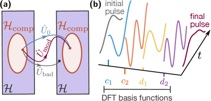
Our generic goal is to use a specific time-dependent Hamiltonian $\hat{H}(t)$ (whose form and tunability is constrained) to produce (at time $t_{\mathrm{f}}$) a desired unitary operation. We start by splitting the Hamiltonian into two parts as $\hat{H}(t)=\hat{H}_{0}(t)+\hat{V}(t)$, where $H_{0}(t)$ is simple enough to be analytically tractable, and $\hat{V}(t)$ represents all the additional interactions that make the problem unsolvable. The basic strategy then has two parts:

1. First, choose control fields in the “simple” Hamiltonian $\hat{H}_{0}(t)$ so that in the absence of $\hat{V}(t)$, one realizes the desired operation. This can be done analytically.

2. Adding back $\hat{V}(t)$ will then destroy the ideal evolution. We address this by modifying available control fields so as to average out the impact of $\hat{V}(t)$. This amounts to adding a control correction to the full Hamiltonian: $\hat{H}(t)\rightarrow\hat{H}(t)+\hat{W}(t)$ [see Fig. 1 (a)].

The question is of course how to find the desired control correction $\hat{W}(t)$. We address this using the strategy described recently in Ref. Ribeiro et al. (2017), where $\hat{W}(t)$ is found perturbatively using a Magnus expansion Magnus (1954); Blanes et al. (2009). A major limitation of this approach is that it often requires terms in $\hat{W}(t)$ that are incompatible with the physical system at hand (e.g. interaction terms that do not exist, or that cannot be made time-dependent in the given experimental platform). This is where the present work makes a substantial contribution. We introduce a novel way to find terms in the series expansion of $\hat{W}(t)$ that are always compatible with all constraints. We achieve this by expanding $\hat{W}(t)$ at each order as a finite sum of time-dependent basis functions multiplied by free weights. Finding the required control corrections then amounts in most cases to solving time-independent linear equations for these weights.

As we demonstrate through several examples, this methodology is both extremely flexible and effective; it can also work in systems with many degrees of freedom. The examples we consider include the strong non-RWA driving of a qubit (Sec. III.1), leakage errors in a superconducting qubit (Sec. III.3), rapid squeezing generation in a parametrically driven bosonic mode (Sec. III.2), and accelerated SNAP gates Heeres et al. (2015); Krastanov et al. (2015) in a coupled transmon-cavity system (Sec. III.4).

Note that the general idea of looking for control fields represented as a finite combination of basis functions was previously used in Refs. Barends et al. (2014); Martinis and Geller (2014) to design two-qubit superconducting qubit gates that minimize leakage errors. In contrast to those works, our work is both more general and more systematic. Our approach is also complementary to a variational approach for approximately finding STA protocols in complex systems that are compatible with experimental constraints Sels and Polkovnikov (2017); Claeys et al. (2019).

II Theoretical Framework

II.1 Imperfect Unitary Evolution

We consider the generic Hamiltonian:

$$\hat{H}(t)=\hat{H}_{0}(t)+\epsilon\hat{V}(t).$$ (1)

The Hamiltonian $\hat{H}_{0}(t)$ generates the desired time evolution, while $\hat{V}(t)$ is the spurious “error” Hamiltonian that disrupts the ideal dynamics and which can be treated as a perturbation. The perturbative character of $\hat{V}(t)$ can originate, e.g., from $\hat{V}(t)$ being proportional to a parameter $\epsilon\ll 1$, or because $\hat{V}(t)$ is a fast oscillating function. In Appendix A we show why nonresonant error-Hamiltonians can also be corrected with the method presented below. In this section, however, we consider the situation where $\hat{V}(t)$ is proportional to a parameter $\epsilon\ll 1$ simply because this allows one to count the orders of the perturbative series in a straightforward way. We stress, however, that one can apply the method that we are about to introduce independently of the reason that makes $\hat{V}(t)$ a perturbation.

The time evolution operator generated by $\hat{H}(t)$ is given by

$$\hat{U}(t)=\hat{U}_{0}(t)\hat{U}_{\mathrm{I}}(t).$$ (2)

Here $\hat{U}_{0}(t)$ represents the ideal time evolution generated by $\hat{H}_{0}(t)$ ($\hbar=1$),

$$\hat{U}_{0}(t)=\hat{T}\exp\left[-i\int_{0}^{t}\mathop{}\!\mathrm{d}t_{1}\hat{H}_{0}(t_{1})\right],$$ (3)

where $\hat{T}$ is the time ordering operator, and we assume that the time evolution starts at $t=0$. The effect of the error Hamiltonian $\hat{V}(t)$ on the dynamics is given by $\hat{U}_{\mathrm{I}}(t)$, which is defined as

$$\hat{U}_{\mathrm{I}}(t)=\hat{T}\exp\left[-i\epsilon\int_{0}^{t}\mathop{}\!\mathrm{d}t_{1}\hat{V}_{\mathrm{I}}(t_{1})\right].$$ (4)

Here, an operator $\hat{O}(t)$ in the interaction picture is given by $\hat{O}_{\mathrm{I}}(t)=\hat{U}_{0}^{\dagger}(t)\hat{O}(t)\hat{U}_{0}(t)$.

Our goal is to have the time evolution operator at $t=t_{\mathrm{f}}$ match a specific desired unitary operator $\hat{U}_{\mathrm{G}}$ ; the form of the time evolution operator at earlier times is not relevant for us. This is the case in many problems, the most prominent example being the engineering of quantum gates. We also assume that $\hat{H}_{0}(t)$ provides us the desired time evolution at $t=t_{\mathrm{f}}$, i.e. $\hat{U}_{0}(t_{\mathrm{f}})=\hat{U}_{\mathrm{G}}$. Consequently, the presence of a non-zero error Hamiltonian $\hat{V}(t)$ disrupts the evolution and prevents us to generate the desired evolution, since in general $\hat{U}_{\mathrm{I}}(t_{\mathrm{f}})\neq\mathbbm{1}$ [see Eq. (2)].

II.2 General Strategy to Correct Unitary Evolution

To obtain the ideal unitary evolution at $t=t_{\mathrm{f}}$, we wish to modify the time-dependence of $\hat{H}(t)$ to cancel the deleterious effects of $\hat{V}(t)$. This is formally accomplished by introducing the modified Hamiltonian

$$\hat{H}_{\mathrm{mod}}(t)=\hat{H}_{0}(t)+\epsilon\hat{V}(t)+\hat{W}(t).$$ (5)

Here, $\hat{W}(t)$ is an unknown control Hamiltonian that cancels, or at least mitigates, the effects of $\hat{V}(t)$ on the dynamics, bringing us closer to the desired time evolution [see Fig. 1 (a)]. The unitary evolution generated by $\hat{H}_{\mathrm{mod}}(t)$ is given by $\hat{U}_{\mathrm{mod}}(t)=\hat{U}_{0}(t)\hat{U}_{\mathrm{mod,\mathrm{I}}}(t)$, where

$$\hat{U}_{\mathrm{mod,\mathrm{I}}}(t)=\hat{T}\exp\left[-i\int_{0}^{t}\mathop{}\!\mathrm{d}t_{1}\hat{H}_{\mathrm{mod,\mathrm{I}}}(t_{1})\right],$$ (6)

is the unitary evolution operator generated by the modified Hamiltonian in the interaction picture with respect to $\hat{H}_{0}(t)$. We have

$$\hat{H}_{\mathrm{mod,\mathrm{I}}}(t)=\epsilon\hat{V}_{\mathrm{I}}(t)+\hat{W}_{\mathrm{I}}(t).$$ (7)

The desired unitary operator at $t=t_{\mathrm{f}}$ is achieved if $\hat{U}_{\mathrm{mod,\mathrm{I}}}(t_{\mathrm{f}})=\mathbbm{1}$, i.e., $\hat{U}_{\mathrm{mod}}(t_{\mathrm{f}})=\hat{U}_{0}(t_{\mathrm{f}})=\hat{U}_{\mathrm{G}}$.

A trivial solution to this problem is to take $\hat{W}(t)=-\epsilon\hat{V}(t)$. This solution is almost always infeasible, as the general form of $\hat{W}(t)$ will be constrained by the kinds of interactions available in the system and their tunability. Furthermore, we are only interested in generating the correct unitary at $t=t_{\mathrm{f}}$ and consequently cancelling the spurious Hamiltonian at all times is in some sense demanding more than it is required. A better solution was found in Ref. Ribeiro et al. (2017), where one makes use of the fact that the time evolution at intermediate times is not important. This leads to relatively lax conditions that the control Hamiltonian $\hat{W}(t)$ must satisfy. Nevertheless, finding an exact $\hat{W}(t)$ is a complex task and generally one needs to resort to perturbation theory to find approximated solutions.

Let us start by writing $\hat{W}(t)$ as a series in $\epsilon$,

$$\hat{W}(t)=\sum\limits_{n=1}^{\infty}\epsilon^{n}\hat{W}^{(n)}(t).$$ (8)

In order to find $\hat{W}(t)$, one could work with the series expansion of the time-ordered exponential of Eq. (6), but a more convenient approach is to use the Magnus expansion Magnus (1954); Blanes et al. (2009). With the Magnus expansion we can convert the complicated time-ordered exponential to a simple exponential of an operator that can be expanded in a series:

$$\hat{U}_{\mathrm{mod,\mathrm{I}}}(t)=\exp\left[\textstyle\sum\limits_{n=1}^{\infty}\hat{\Omega}_{n}(t)\right].$$ (9)

The terms of the Magnus expansion, $\hat{\Omega}_{k}(t)$, are recursively defined by differential equations Magnus (1954); Blanes et al. (2009), with the first two terms being given by (see also Appendix B)

$$\partial_{t}\hat{\Omega}_{1}(t) =-i\hat{H}_{\mathrm{mod,\mathrm{I}}}(t),$$ (10)

$$\partial_{t}\hat{\Omega}_{2}(t) =\frac{1}{2}[\partial_{t}\hat{\Omega}_{1}(t),\hat{\Omega}_{1}(t)].$$ (11)

In order to correct the dynamics up to order $\mathcal{O}(\epsilon^{m})$, one needs to find a control Hamiltonian $\hat{W}(t)$ such that $\hat{\Omega}_{k}(t_{\mathrm{f}})=\mathbf{0}$ for $k=1,\ldots,m$. As shown in Ref. Ribeiro et al. (2017) this is accomplished if one firstly truncates the series representing $\hat{W}(t)$ [see Eq. (8)] up to order $m$ and then requires the operators $\hat{W}^{(n)}_{\mathrm{I}}(t)$ to satisfy the following equations:

$$\epsilon^{n}\int_{0}^{t_{\mathrm{f}}}\mathop{}\!\mathrm{d}t\ \hat{W}^{(n)}_{\mathrm{I}}(t)=-i\sum_{k=1}^{n}\hat{\Omega}_{k}^{(n-1)}(t_{\mathrm{f}}),$$ (12)

where $\hat{\Omega}_{k}^{(n)}(t)$ is the kth term of the Magnus expansion associated to the partially-corrected Hamiltonian

$$\hat{H}_{\mathrm{mod,\mathrm{I}}}^{(n)}(t)=\epsilon\hat{V}_{\mathrm{I}}(t)+\sum_{k=1}^{n}\epsilon^{k}\hat{W}^{(k)}_{\mathrm{I}}(t).$$ (13)

Here, the series representing the correction $\hat{W}(t)$ has been truncated at order $n$.

To first order ($k=1$), Eq. (12) reduces to

$$\int_{0}^{t_{\mathrm{f}}}\mathop{}\!\mathrm{d}t\ \hat{W}^{(1)}_{\mathrm{I}}(t)=-\int_{0}^{t_{\mathrm{f}}}\mathop{}\!\mathrm{d}t\ \hat{V}_{\mathrm{I}}(t).$$ (14)

Equation (12) is the only restriction on the terms of the control Hamiltonian $\hat{W}(t)$. This implies we have considerable latitude in how we make our specific choice of $\hat{W}(t)$. In what follows we fully exploit this freedom to systematically find control Hamiltonians that are completely compatible with experimental constraints on kinds and tunability of available interactions.

II.3 Constrained Control Hamiltonians

To proceed, we introduce a set of $N_{\mathrm{op}}$ time-independent Hermitian operators $\{\hat{A}_{j}\}$ that form a basis for $\hat{H}_{0}(t)$, $\hat{V}(t)$, and $\hat{W}(t)$. By this, we mean that these operators allow for a unique decomposition of the different Hamiltonian operators at each instant of time:

$$\hat{H}_{0}(t) =\sum\limits_{j}h_{j}(t)\hat{A}_{j},$$ (15)

$$\hat{V}(t) =\sum\limits_{j}v_{j}(t)\hat{A}_{j},$$ (16)

$$\hat{W}(t) =\sum\limits_{j}w_{j}(t)\hat{A}_{j}.$$ (17)

Here $h_{j}(t)$, $v_{j}(t)$, and $w_{j}(t)$ are the real control fields (expansion coefficients) associated with the decomposition of $\hat{H}_{0}(t)$, $\hat{V}(t)$, and $\hat{W}(t)$, respectively. For instance, the elements of the set $\{\hat{A}_{j}\}$ for a two-level system are the Pauli operators $\hat{\sigma}_{j}$ with $j\in\{1,3\}$. We also introduce the Lie algebra $\mathfrak{g}$ generated by the set of operators $\{-i\hat{A}_{j}\}$ with the Lie bracket given by the commutation operation. Having a Lie algebra ensures that one can use the basis formed by the set $\{\hat{A}_{j}\}$ to decompose the operators generated by the Magnus expansion. Finally, we stress that $N_{\mathrm{op}}$ can be finite even if the dimension of the Hilbert space is infinite. This is the case for quadratic bosonic forms that can be characterized by the special unitary groups SU$(2)$ or SU$(1,1)$, which are associated to the Lie algebras su$(2)$ or su$(1,1)$ Yurke et al. (1986).

Transforming Eqs. (16) and (17) to the interaction picture defined by $\hat{H}_{0}(t)$, we have

$$\hat{V}_{\mathrm{I}}(t)=\sum\limits_{j}v_{j}(t)\hat{A}_{j,\mathrm{I}}.$$ (18)

Using the fact that $\{\hat{A}_{j}\}$ forms a basis, we can write

$$\hat{A}_{j,\mathrm{I}}=\sum\limits_{l}a_{j,l}(t)\hat{A}_{l}.$$ (19)

Here, the functions $a_{j,l}(t)$ fully encode the action of the interaction picture transformation on our basis operators.

Substituting Eq. (19) in Eq. (18), we obtain

$$\hat{V}_{\mathrm{I}}(t)=\sum\limits_{j}\tilde{v}_{j}(t)\hat{A}_{j},$$ (20)

where we use tildes to denote control fields in the interaction picture, and we have

$$\tilde{v}_{j}(t)=\sum\limits_{l}a_{l,j}(t)v_{l}(t).$$ (21)

Proceeding analogously for $\hat{W}(t)$ and using the series representation defined in Eq. (8), we get

$$\hat{W}_{\mathrm{I}}^{(n)}(t)=\sum\limits_{j}\tilde{w}_{j}^{(n)}(t)\hat{A}_{j},$$ (22)

with

$$\tilde{w}_{j}^{(n)}(t)=\sum\limits_{l}a_{l,j}(t)w_{l}^{(n)}(t).$$ (23)

We now return to the fundamental equations of our approach, Eqs. (12), which need to be satisfied to cancel the effects of $\hat{V}(t)$ to the desired order. As written, these equations do not reflect any information about relevant experimental constraints. Typical examples of constraints are the inability to control the fields that couple to certain $\hat{A}_{j}$, i.e. that particular field has to obey $w_{j}^{(n)}(t)=0$. Note that in general it is possible to have $h_{j}(t)\neq 0$ while one must work with the condition $w_{j}^{(n)}(t)=0$. Moreover, even if $w_{j}^{(n)}(t)$ can be controlled, it might have restrictions, e.g. $w_{j}^{(n)}$ must be time independent or has bandwidth limitations. In the following we show how to derive equations for $w_{j}^{(n)}(t)$ that obey Eqs. (12) and simultaneously fulfill the previously mentioned constraints. This then enables the design of high fidelity control pulses that are fully compatible with experimental constraints. As we discuss below, it is enough to show how one derives equations for the first-order control fields $w_{j}^{(1)}(t)$, which must obey Eq. (14), since the procedure for $w_{j}^{(n)}(t)$ is similar.

We proceed by substituting Eqs. (20) and (22) into Eq. (14), which determines the first-order correction Hamiltonian. We obtain an operator equation which can be split into $N_{\mathrm{op}}$ equations, one for each operator $\hat{A}_{j}$:

$$\int_{0}^{t_{\mathrm{f}}}\mathop{}\!\mathrm{d}t\tilde{w}_{j}^{(1)}(t)=-\int_{0}^{t_{\mathrm{f}}}\mathop{}\!\mathrm{d}t\tilde{v}_{j}(t).$$ (24)

We stress that Eq. (24) may be ill-defined since it is possible to have $\tilde{w}_{j}^{(1)}(t)=0$ while $\tilde{v}_{j}(t)\neq 0$ for certain values of $j$. We show in Sec. III.4 how to deal with such situations for a large class of problems. For the remainder of this section, we focus on the simpler case where we have a well-defined system of equations.

The problem still remains of how to solve for $w_{j}^{(1)}(t)$; this is still a complex task since one is dealing with a system of $N_{\mathrm{op}}$ coupled integral equations. This problem can be overcome by choosing an appropriate parametrization for the functions $w_{j}^{(1)}(t)$. Here, since $w_{j}^{(1)}(t)$ must only have support on the interval $[0,t_{\mathrm{f}}]$, we use a finite Fourier series decomposition,

$$w_{j}^{(1)}(t)=\sum\limits_{k=0}^{k_{\mathrm{max}}}c_{jk}^{(1)}\cos\left(\omega_{k}t\right)+d_{jk}^{(1)}\sin\left(\omega_{k}t\right),$$ (25)

with $\omega_{k}=2\pi k/t_{\mathrm{f}}$ and $d_{j0}^{(1)}=0$. This parametrization allows us to carry out the time integration over the duration of the protocol and use the Fourier coefficients as the free parameters to satisfy the system of equations given by Eq. (24). We stress that at this stage finding the first order correction that fulfills Eq. (14) has been reduced to determining a set of $N_{\mathrm{coeffs}}=N_{\mathrm{op}}\times(2k_{\mathrm{max}}+1)$ coefficients. Note that one could use other basis functions for the decomposition, e.g., Slepian functions Slepian and Pollak (1961).

The sum in Eq. (25) runs from $0$ to $k_{\mathrm{max}}$ which allows us to limit the bandwidth of the field associated to $\hat{A}_{j}$. We also note that $k_{\mathrm{max}}$ can take different values for different values of $j$. For constrained systems where a particular field $w_{j}(t)$ must be time independent, we set all the coefficients in Eq. (25) to zero with the exception of $c_{j0}$. If one requires $w_{j}^{(1)}(0)=w_{j}^{(1)}(t_{\mathrm{f}})=0$, then one finds using Eq. (25) that the coefficients $c_{jk}^{(1)}$ must obey $\sum_{k=0}^{k_{\mathrm{max}}}c_{jk}^{(1)}=0$. For simplicity the summation in Eq. (25) runs from $0$ to $k_{\mathrm{max}}$, but the more general case where the summation runs from $k_{\mathrm{min}}$ to $k_{\mathrm{max}}$ is also allowed.

We now can formulate the final basic equations of our approach. We substitute Eqs. (23) and (25) in the system of equations defined by Eq. (24). Since we know the explicit time dependence of $\tilde{w}_{j}^{(1)}(t)$, we can perform the time integration. This leads to a system of time-independent $N_{\mathrm{op}}$ linear equations than can be written in matrix form:

$$M\>\mbox{\boldmath$x$}^{(1)}=\mbox{\boldmath$y$}^{(1)}.$$ (26)

Here, $\mbox{\boldmath$x$}^{(1)}$ is a vector of coefficients (length $N_{\mathrm{coeffs}}$) determining the first order control correction that we are trying to find. In contrast, the matrix $M$ and the vector $\mbox{\boldmath$y$}^{(1)}$ are known quantities: $\mbox{\boldmath$y$}^{(1)}$ parameterizes the error Hamiltonian $\hat{V}(t)$, whereas $M$ encodes the dynamics of the ideal evolution generated by $\hat{H}_{0}(t)$.

To be more explicit, the $\mbox{\boldmath$y$}^{(1)}$ is a vector of length $N_{\mathrm{op}}$ whose components are the spurious error-Hamiltonian elements we wish to average out,

$$y^{(1)}_{j}=-\int_{0}^{t_{\mathrm{f}}}\mathop{}\!\mathrm{d}t\tilde{v}_{j}(t).$$ (27)

$\mbox{\boldmath$x$}^{(1)}$ is the vector of the $N_{\mathrm{coeffs}}$ unknown Fourier coefficients $c_{lk}^{(1)}$ and $d_{lk}^{(1)}$ that determine our control corrections, c.f. Eq. (25). We order these as follows

$$x^{(1)}_{j}=\begin{cases}c_{lk}^{(1)}&\text{if }j\leq j_{0},\\ d_{lk}^{(1)}&\text{if }j>j_{0},\end{cases}$$ (28)

where $j_{0}=N_{\mathrm{op}}(k_{\mathrm{max}}+1)$, and the indices $l$ and $k$ in Eq. (28) are functions of $j$. We have

$$l=\begin{dcases}(j-1)//(k_{\mathrm{max}}+1)+1&\text{if }j\leq j_{0},\\ (j-j_{0}-1)//k_{\mathrm{max}}+1&\text{if }j>j_{0},\end{dcases}$$ (29)

and

$$k=\begin{dcases}(j-1)\%(k_{\mathrm{max}}+1)&\text{if }j\leq j_{0},\\ (j-j_{0}-1)\%k_{\mathrm{max}}+1&\text{if }j>j_{0}.\end{dcases}$$ (30)

Here, $a//b$ denotes the integer division of $a$ by $b$ and $a\%b$ denotes the remainder of the integer division of $a$ by $b$.

Finally, $M$ is a $(N_{\mathrm{op}}\times N_{\mathrm{coeffs}})$ matrix that characterizes the evolution under the ideal Hamiltonian $\hat{H}_{0}(t)$. Recall that the interaction picture transformation generated by this Hamiltonian is described by the functions $a_{jl}(t)$. The matrix elements of $M$ involve the Fourier series of these functions [see Eq. (19)]:

$$M_{ij}=\begin{dcases}\displaystyle\int_{0}^{t_{\mathrm{f}}}\mathop{}\!\mathrm{d}t\ a_{l,i}(t)\cos(\omega_{k}t)&\text{if }j\leq j_{0},\\ \displaystyle\int_{0}^{t_{\mathrm{f}}}\mathop{}\!\mathrm{d}t\ a_{l,i}(t)\sin(\omega_{k}t)&\text{if }j>j_{0},\end{dcases}$$ (31)

where $l$ and $k$ are given by Eqs. (29) and (30), respectively. We stress that Eqs. (27) to (31) are valid when the summation in Eq. (25) runs from $0$ to $k_{\mathrm{max}}$ for all values of $j$, but they can be modified to describe other cases.

Higher orders controls are found with an identical procedure. Ultimately, each order is found by solving a system of time-independent $N_{\mathrm{op}}$ linear equations similar to Eq. (26) [see Appendix C].

In principle, a set of constrained controls fields that allows one to correct the dynamics up to order $n$, does not necessarily allows one to correct the dynamics up to order $n+1$. In such situations, namely when the obtained linear system does not have a solution , one usually has to choose another correction Hamiltonian for the system. There are cases, however, where an alternative solution can be found. We illustrate this situation when we discuss the SNAP problem in Sec. III.4.

Symbol	Meaning		Equation
$\hat{H}_{0}(t)$	Ideal Hamiltonian		Eq. (1)
$\hat{V}(t)$	Spurious “error” Hamiltonian		Eq. (1)
$\hat{W}^{(k)}(t)$	kth order correction Hamiltonian		Eq. (8)
$\hat{O}_{\mathrm{I}}$	Operator in the interaction picture with respect to $\hat{H}_{0}(t)$		-
$\hat{\Omega}_{j}(t)$	$j$-th Magnus operator associated with $\hat{V}_{\mathrm{I}}(t)$		Eq. (9)
$\hat{\Omega}_{j}^{(k)}(t)$	jth Magnus operator associated with the modified Hamiltonian		Eq. (13)
$\hat{A}_{j}$	Basis operator of the Hilbert space		-
$v_{j}(t)$	Decomposition coefficients of $\hat{V}(t)$		Eq. (16)
$w_{j}^{(n)}(t)$	Decomposition coefficients of $\hat{W}^{(n)}(t)$		Eq. (17)
$a_{l,j}(t)$	Decomposition coefficients of $\hat{A}_{l,\mathrm{I}}(t)$		Eq. (19)
$\tilde{v}_{j}(t)$	Decomposition coefficients of $\hat{V}_{\mathrm{I}}(t)$		Eq. (20)
$\tilde{w}_{j}(t)$	Decomposition coefficients of $\hat{W}_{\mathrm{I}}(t)$		Eq. (22)
$c_{jk},d_{jk}$	Fourier coefficients of $w_{j}(t)$		Eq. (25)

Table 1: Definition of the most important symbols.

III Applications

In this section, we apply our general strategy to several experimentally relevant problems. These examples highlight the fact that our method is broadly applicable (without modification) to a wide range of very diverse problems.

III.1 Strong Driving of a Two-Level System

As a first example we consider the problem of a two-level system (qubit) in the strong driving limit. As we discuss below, this regime generates a complex dynamics that renders precise control of the qubit hard to achieve. Several techniques were used to predict control schemes which generate high-fidelity gates. Optimal control methods have been used, but the resulting control fields are not bandwidth limited and cannot be accurately reproduced by an arbitrary wave form generator Scheuer et al. (2014). An ad hoc method based on time optimal control of a two-level system Boscain and Mason (2006); Garon et al. (2013) was also proposed: it consists in realizing Bang-Bang control with imperfect square control fields Hirose and Cappellaro (2018). However, to achieve a gate with a reasonably low error the imperfect square pulse must still have a relatively large bandwidth. A method based on analyzing the dynamics of the system using Floquet theory has also been put forward Deng et al. (2015, 2016), but this transforms a low dimensional control problem into a high dimensional one.

Figure 2: Modified dynamics of a qubit in the strong driving limit. (a) Average fidelity error for a Hadamard gate as a function of gate time. The blue trace is calculated using the uncorrected Hamiltonian [see Eq. (32)]. The green trace is obtained for the modified Hamiltonian (up to second order). (b) Coefficient of the of original pulse $f_{\mathrm{q}}(t)$ and the coefficients of the correction Hamiltonian as a function of the gate time. Here $c_{\alpha,1}=c_{\alpha,1}^{(1)}+c_{\alpha,2}^{(2)}$ and $\Delta=\Delta^{(1)}+\Delta^{(2)}$. (c-d) Original pulse and corrected pulse for $\omega_{\mathrm{d}}t_{f}\approx 5$. In (c) we plot $f_{\mathrm{q},x}^{(n)}(t)$ while in (d) we plot $f_{\mathrm{q},y}^{(n)}(t)$ [see Eq. (52)]. (e) Trajectory on the Bloch sphere of the ideal dynamics (grey), of the uncorrected dynamics (blue), and of the corrected dynamics (orange).

The Hamiltonian of a driven two-level system is given by

$$\hat{H}_{\mathrm{qubit}}(t)=\frac{\omega_{\mathrm{q}}}{2}\hat{\sigma}_{z}+f_{\mathrm{q}}(t)\cos(\omega_{\mathrm{d}}t)\hat{\sigma}_{x},$$ (32)

where $\omega_{\mathrm{q}}$ is the qubit splitting frequency, $\omega_{\mathrm{d}}$ is the driving frequency, $f_{\mathrm{q}}(t)$ is the driving envelope, and we introduce the Pauli operators:

$$\hat{\sigma}_{x} =|0\rangle\!\langle 1|+|1\rangle\!\langle 0|,$$ (33)

$$\hat{\sigma}_{y} =i|0\rangle\!\langle 1|-i|1\rangle\!\langle 0|,$$

$$\hat{\sigma}_{z} =|1\rangle\!\langle 1|-|0\rangle\!\langle 0|.$$

We label by $|0\rangle$ and $|1\rangle$ the ground and excited states of the system, respectively. We note that the Pauli operators (multiplied by the imaginary number $-i$) define a Lie algebra with respect to the commutation operation.

In the weak driving limit, i.e. $f_{\mathrm{q}}(t)\ll\omega_{\mathrm{d}}\,\forall t$, Eq. (32) allows one to generate rotations around the $x$-axis if one sets $\omega_{\mathrm{d}}=\omega_{\mathrm{q}}$. This is best understood in the frame rotating at the drive frequency . In this frame the Hamiltonian is given by $\hat{H}_{\mathrm{R}}(t)=\hat{H}_{\mathrm{q},0}(t)+\hat{V}_{\mathrm{q}}(t)$ with

$$\hat{H}_{\mathrm{q},0}(t)=\frac{f_{\mathrm{q}}(t)}{2}\hat{\sigma}_{x},$$ (34)

and

$$\hat{V}_{\mathrm{q}}(t)=v_{\mathrm{q},x}(t)\hat{\sigma}_{x}+v_{\mathrm{q},y}(t)\hat{\sigma}_{y}.$$ (35)

The coefficients $v_{\mathrm{q},j}(t)$ are given by

$$v_{\mathrm{q},x}(t) =\frac{f_{\mathrm{q}}(t)}{2}\cos(2\omega_{\mathrm{d}}t),$$ (36)

$$v_{\mathrm{q},y}(t) =-\frac{f_{\mathrm{q}}(t)}{2}\sin(2\omega_{\mathrm{d}}t).$$

Here, the driving is set on resonance with the qubit frequency, i.e., $\omega_{\mathrm{q}}=\omega_{\mathrm{d}}$. If the system is in the weak driving limit, the fast oscillating terms (also known as counter-rotating terms) in $\hat{V}_{\mathrm{q}}(t)$ can be neglected as they average themselves out over the long evolution time set by the slow varying envelope function $f_{\mathrm{q}}(t)$. As a consequence, one can approximate $\hat{H}_{\mathrm{R}}(t)$ by $\hat{H}_{\mathrm{q},0}(t)$. This is known as the rotating wave approximation (RWA). The resulting Hamiltonian generates a rotation of angle $\theta(t_{\mathrm{f}})$ around the $x$-axis, where we have introduced

$$\theta(t)=\int_{0}^{t}\mathop{}\!\mathrm{d}t_{1}\ f_{\mathrm{q}}(t_{1}).$$ (37)

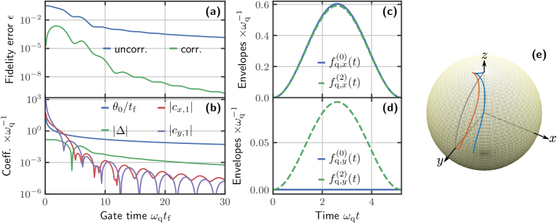
However, when one deviates from the weak driving limit, the counter-rotating terms cannot be neglected anymore since they do not average themselves out on short evolution times. As a result, the dynamics generated by $\hat{H}_{\mathrm{R}}(t)$ describes a complex rotation around a time-dependent axis evolving in the $xy$-plane of an angle which is no more accurately described by Eq. (37) Bloch and Siegert (1940) [see Fig. 2 (e)]. To this day there is no known exact solution to this problem, which makes the strong-driving limit impractical to control a qubit with high-fidelity. However, using the general framework laid out in Sec. II, we can mitigate the effects of $\hat{V}_{\mathrm{q}}(t)$ in situations where the RWA breaks down. This allows us to generate any high-fidelity single-qubit gate beyond the RWA regime.

Given the constraints of the original problem, i.e., we only have temporal control over a field coupling to $\hat{\sigma}_{x}$ [see Eq. (32)], we look for a correction of the form

$$\hat{W}_{\mathrm{qubit}}(t)= \sum\limits_{n}\left[g_{x}^{(n)}(t)\cos(\omega_{\mathrm{d}}t)+g_{y}^{(n)}(t)\sin(\omega_{\mathrm{d}}t)\right]\hat{\sigma}_{x}.$$ (38)

Here, $g_{x}^{(n)}(t)$ and $g_{y}^{(n)}(t)$ are unknown envelope functions. In addition to the driving field, we also have the liberty to choose the driving frequency; nothing tells us that having $\omega_{\mathrm{d}}=\omega_{\mathrm{q}}$ is the best thing to do in terms of control beyond the RWA. In the rotating frame, this is equivalent to have a non-zero detuning $\Delta=\omega_{\mathrm{q}}-\omega_{\mathrm{d}}$. Therefore, we consider the following modified Hamiltonian in the rotating frame

$$\hat{H}_{\mathrm{R},\mathrm{mod}}(t)=\hat{H}_{\mathrm{q},0}(t)+\hat{V}_{\mathrm{q}}(t)+\sum\limits_{n}\hat{W}_{\mathrm{q}}^{(n)}(t).$$ (39)

In terms of the Pauli operators, $\hat{W}_{\mathrm{q}}^{(n)}(t)$ is given by

$$\hat{W}_{\mathrm{q}}^{(n)}(t)=w_{\mathrm{q},x}^{(n)}(t)\hat{\sigma}_{x}+w_{\mathrm{q},y}^{(n)}(t)\hat{\sigma}_{y}+w_{\mathrm{q},z}^{(n)}(t)\hat{\sigma}_{z},$$ (40)

with

$$w_{\mathrm{q},x}^{(n)}(t) =g^{(n)}(t)\cos(\omega_{\mathrm{d}}t),$$ (41)

$$w_{\mathrm{q},y}^{(n)}(t) =-g^{(n)}(t)\sin(\omega_{\mathrm{d}}t),$$

$$w_{\mathrm{q},z}^{(n)}(t) =\Delta^{(n)}.$$

In practice, having a control field with two-quadratures driving [see Eq. (38)] and introducing a detuning has given us the ability to implement $3$-axes control. We stress that there are other possible choices for $\hat{W}(t)$, but they all require more resources to be implemented experimentally [see Appendix D.1]. Note that the modified detuning is given by $\Delta=\sum_{n}\Delta^{(n)}$ in complete analogy to having the control fields represented by a series [see Eq. (8)].

Following the general strategy presented in Sec. II, we first move to the interaction picture with respect to $\hat{H}_{\mathrm{q},0}(t)$ [see Eq. (34)]. In the interaction picture, $\hat{V}_{\mathrm{q}}(t)$ [see Eq. (35)] and the control Hamiltonian $\hat{W}_{\mathrm{q}}^{(n)}(t)$ [see Eq. (40)] are respectively given by

$$\hat{V}_{\mathrm{q},\mathrm{I}}(t)=\tilde{v}_{\mathrm{q},x}(t)\hat{\sigma}_{x}+\tilde{v}_{\mathrm{q},y}(t)\hat{\sigma}_{y}+\tilde{v}_{\mathrm{q},z}(t)\hat{\sigma}_{z},$$ (42)

with

$$\tilde{v}_{\mathrm{q},x}(t) =\frac{f_{\mathrm{q}}(t)}{2}\cos(2\omega_{\mathrm{d}}t),$$ (43)

$$\tilde{v}_{\mathrm{q},y}(t) =-\frac{f_{\mathrm{q}}(t)}{2}\sin(2\omega_{\mathrm{d}}t)\cos{\theta},$$

$$\tilde{v}_{\mathrm{q},z}(t) =\frac{f_{\mathrm{q}}(t)}{2}\sin(2\omega_{\mathrm{d}}t)\sin{\theta},$$

and

$$\hat{W}_{\mathrm{q},\mathrm{I}}^{(n)}(t)=\tilde{w}_{\mathrm{q},x}^{(n)}(t)\hat{\sigma}_{x}+\tilde{w}_{\mathrm{q},y}^{(n)}(t)\hat{\sigma}_{y}+\tilde{w}_{\mathrm{q},z}^{(n)}(t)\hat{\sigma}_{z}$$ (44)

with

$$\tilde{w}_{\mathrm{q},x}^{(n)}(t) =g^{(n)}(t)\cos(\omega_{\mathrm{d}}t),$$ (45)

$$\tilde{w}_{\mathrm{q},y}^{(n)}(t) =-g^{(n)}(t)\sin(\omega_{\mathrm{d}}t)\cos{\theta}+\Delta^{(n)}\sin{\theta},$$

$$\tilde{w}_{\mathrm{q},z}^{(n)}(t) =g^{(n)}(t)\sin(\omega_{\mathrm{d}}t)\sin{\theta}+\Delta^{(n)}\cos{\theta}.$$

In Eqs. (43) and (45), we have omitted the explicit time dependence of $\theta$ for simplicity, i.e., $\theta=\theta(t)$ [see Eq. (37)]. The next step consists in expanding the control fields $\tilde{w}_{\mathrm{q},j}^{(n)}(t)$ ($j\in\{x,y,z\}$) [see Eq.(45)] into a Fourier series. However, before proceeding it is useful to notice the special form of the functions $\tilde{w}_{\mathrm{q},j}^{(n)}(t)$: an unknown function that multiplies a known fast oscillating function. It is therefore more suitable to just expand the unknown functions $g_{x}^{(n)}(t)$, $g_{y}^{(n)}(t)$ [see Eq. (38)], and $\Delta^{(n)}$ in a Fourier series and use the corresponding Fourier coefficients as the free parameters to satisfy the system of equations generated by the Magnus-based approach. We stress, however, that one obtains exactly the same results using the general procedure of Sec. II and imposing the necessary constraints on the Fourier series.

If we constrain $g_{\alpha=x,y}^{(n)}(t)$ to be zero at $t=0$ and $t=t_{\mathrm{f}}$, which is often the case experimentally, we obtain the following Fourier expansions

$$g_{\alpha}^{(n)}(t)=\sum\limits_{k=1}^{\infty}c_{\alpha,k}^{(n)}\left[1-\cos(\omega_{k}t)\right]+d_{\alpha,k}^{(n)}\sin(\omega_{k}t),$$ (46)

and

$$\Delta^{(n)}=c_{z,0}^{(n)}+\textstyle\sum\limits_{k=1}^{\infty}c_{z,k}^{(n)}\cos(\omega_{k}t)+d_{z,k}^{(n)}\sin(\omega_{k}t),$$ (47)

where $\omega_{k}=2\pi/t_{\mathrm{f}}$. Since we have a total of three equations of the form of Eq. (24) to solve (one for each Pauli operator), we need at least three free parameters. Consequently, we can set all coefficients to zero in Eqs. (46) and (47) except $c_{x,1}^{(n)}$, $c_{y,1}^{(n)}$ and $c_{z,0}^{(n)}$ . With this choice, Eqs. (46) and (47) reduce to

$$g_{\alpha=x,y}^{(n)}(t)=c_{\alpha,1}^{(n)}\left[1-\cos(\omega_{1}t)\right],$$ (48)

and

$$\Delta^{(n)}=c_{z,0}^{(n)}.$$ (49)

The final step is to find the value of the free parameters $c_{x,1}^{(n)}$, $c_{y,1}^{(n)}$ and $\Delta^{(n)}$. We start by verifying that by substituting Eqs. (48) and (49) in Eq. (44), we obtain a correction Hamiltonian $\hat{W}_{\mathrm{q},\mathrm{I}}^{(n)}(t)$ [see Eq. (44)] that depends, as desired, linearly on the free parameters $c_{x,1}^{(n)}$, $c_{y,1}^{(n)}$ and $\Delta^{(n)}$. The system of equations defining the first order coefficients [$n=1$, see Eq. (26)], is given by

$$P_{\mathrm{q}}\mbox{\boldmath$x$}_{\mathrm{q}}^{(1)}=\mbox{\boldmath$y$}_{\mathrm{q}}^{(1)},$$ (50)

where $\mbox{\boldmath$x$}_{\mathrm{q}}^{(1)}=\{c_{x,1}^{(1)},c_{y,1}^{(1)},\Delta^{(1)}\}^{T}$ is the vector of unknown coefficients [see Eq. (28)], $\mbox{\boldmath$y$}_{\mathrm{q}}^{(1)}=-\int_{0}^{t_{\mathrm{f}}}\mathop{}\!\mathrm{d}t\{\tilde{v}_{\mathrm{q},x}(t),\tilde{v}_{\mathrm{q},y}(t),\tilde{v}_{\mathrm{q},z}(t)\}^{T}$ is the vector of the spurious error-Hamiltonian elements with $\tilde{v}_{\mathrm{q},j}(t)$ ($j\in\{x,y,z\}$) defined in Eq. (43), and $P_{\mathrm{q}}$  is the matrix that characterizes the evolution under the ideal Hamiltonian $\hat{H}_{\mathrm{q},0}(t)$ [see Eq. (34)]. The explicit matrix elements of $P_{\mathrm{q}}$ can be found in Appendix D.2. Higher-order correction Hamiltonians can be found in a similar way.

In Fig. 2 (a), we plot the average fidelity error $\varepsilon$ Pedersen et al. (2007) for a Hadamard gate generated with an initial envelope

$$f_{\mathrm{q}}(t)=\frac{\theta_{0}}{t_{\mathrm{f}}}\left[1-\cos\left(\frac{2\pi t}{t_{\mathrm{f}}}\right)\right],$$ (51)

with $\theta_{0}=\pi/2$. Other gates can be realized by choosing $\theta_{0}\in[0,2\pi]$. The blue trace shows the error for the uncorrected evolution while the green trace shows the error of the corrected evolution up to second order. The latter, as one can observe in Fig. 2 (a), globally increases when $\omega_{\mathrm{q}}t_{\mathrm{f}}$ decreases, but around $\omega_{\mathrm{q}}t_{\mathrm{f}}\simeq 1$ the error of the corrected evolution starts decreasing again. This can be understood by considering the limit $t_{\mathrm{f}}\to 0$ ($\omega_{\mathrm{q}}t_{\mathrm{f}}\to 0$). In this limit, we have $\tilde{v}_{\mathrm{q},x}(t)\to f_{\mathrm{q}}(t)/2$ and $\tilde{v}_{\mathrm{q},y}(t)=\tilde{v}_{\mathrm{q},z}(t)\to 0$ [See Eq. (43)] which implies that $\hat{V}_{\mathrm{I}}(t)$ commutes with itself at all times. As a consequence, one can find exact modifications to the control fields since only the first order of the Magnus expansion is non-zero. However, as one can see in Fig. 2 (b), where we plot the coefficients of the correction versus the gate time $t_{\mathrm{f}}$, the modified control sequences require control fields with diverging amplitudes. Restricting ourselves to gate times close to unity ($\omega_{\mathrm{q}}t_{\mathrm{f}}\simeq 1$), where the modified control sequences can be experimentally realized, our strategy improves the error $\varepsilon$ by more than two orders of magnitude. In Figs. 2 (c) and (d), we compare the original and corrected pulses for $\omega_{\mathrm{q}}t_{\mathrm{f}}\approx 5$. One can observe that the changes to the original pulse are small. For convenience we write the nth order modified pulse as

$$f_{\mathrm{\mathrm{q},mod}}(t)=f_{\mathrm{q},x}^{(n)}(t)\cos(\omega_{\mathrm{q}}t)+f_{\mathrm{q},y}^{(n)}(t)\sin(\omega_{\mathrm{q}}t),$$ (52)

where $f_{\mathrm{q},x}^{(n)}(t)=f_{\mathrm{q}}(t)+\sum_{k=1}^{n}g_{x}^{(n)}(t)$ and $f_{\mathrm{q},y}^{(n)}(t)=\sum_{k=1}^{n}g_{y}^{(n)}(t)$. When $n=0$ we have simply the original pulse, thus $f_{\mathrm{q},x}^{(0)}(t)=f_{\mathrm{q}}(t)$ and $f_{\mathrm{q},y}^{(0)}(t)=0$.

Figure 3: Fast generation of intra-cavity squeezing. (a) Intra-cavity squeezing as a function of the total evolution time. The red trace corresponds to the ideal case where the fast oscillating terms have been neglected. The blue trace shows the squeezing when the fast oscillating terms are present and no correction is used. The green trace shows the squeezing with the modified Hamiltonian (up to sixth order). (Inset) Angle in the phase space where the squeezing is maximal as a function of gate time. The ideal case is $\Delta\varphi=0$. (b) Coefficients of the correction Hamiltonian as a function the total evolution time: $\{c_{x,1},\ c_{y,1},\ \Delta\}=\sum_{n=1}^{3}\{c_{x,1}^{(n)},\ c_{y,1}^{(n)},\ \Delta^{(n)}\}$.

III.2 Strong driving of a Parametrically Driven Cavity

As a second example, we consider the problem of fast generation of squeezed states using a parametrically driven cavity (PDC). The ability to generate squeezed states with quantum oscillators is of particular interest since it allows one, among others, to enhance sensing capabilities Burd et al. (2019) or to reach the single-photon strong coupling regime with optomechanical systems using only linear resources Lemonde et al. (2016). Recently, optimal control techniques have been used to achieve squeezing of an optomechanical oscillator at finite temperature Basilewitsch et al. (2019).

Here, we are interested in generating squeezing on a relatively short time scale by using a pulsed drive. As for the qubit problem discussed in Sec. III.1, this turns out to be a complex task due to fast counter-rotating terms that prevent the preparation of the desired squeezed state.

The Hamiltonian of a PDC corresponds to having a harmonic oscillator with a modulated spring constant. This can be achieved, e.g., in the microwave regime by modulating the magnetic flux through a SQUID loop (flux-pumped Josephson parametric amplifier) Ojanen and Salo (2007); Yamamoto et al. (2008). We have

$$\hat{H}_{\mathrm{PDC}}(t)=\omega_{\mathrm{a}}\hat{a}^{\dagger}\hat{a}+f_{\mathrm{D}}(t)\sin(\omega_{\mathrm{d}}t)\left(\hat{a}+\hat{a}^{\dagger}\right)^{2},$$ (53)

with $\hat{a}$ ($\hat{a}^{\dagger}$) the bosonic annihilation (creation) operator. The frequency of the mode $\hat{a}$ is $\omega_{\mathrm{a}}$ and the drive has frequency $\omega_{\mathrm{d}}$.

It is convenient to introduce the operators Yurke et al. (1986)

$$\hat{\mu}_{x} =\frac{1}{2}\left(\hat{a}^{2}+\hat{a}^{\dagger 2}\right),$$ (54)

$$\hat{\mu}_{y} =-\frac{i}{2}\left(\hat{a}^{2}-\hat{a}^{\dagger 2}\right),$$

$$\hat{\mu}_{z} =\frac{1}{2}\left(\hat{a}^{\dagger}\hat{a}+\hat{a}\hat{a}^{\dagger}\right),$$

which define (multiplied by the imaginary number $-i$) a Lie algebra with respect to the commutation operation [see Appendix E.1]. As mentioned earlier, since the Hamiltonian is quadratic, the three operators defined in Eq. (54) are enough to completely describe the full dynamics in spite of having an infinite Hilbert space. The action of these operators is best understood in the phase space defined by $\hat{x}=(\hat{a}+\hat{a}^{\dagger})/\sqrt{2}$ and $\hat{y}=-i(\hat{a}-\hat{a}^{\dagger})/\sqrt{2}$: $\hat{\mu}_{x}$ generates squeezing along the $x$-axis, $\hat{\mu}_{y}$ generates squeezing along the $y$-axis, and $\hat{\mu}_{z}$ generates a rotation around the origin of the phase space.

In a frame rotating at a frequency $\omega_{\mathrm{d}}/2=\omega_{\mathrm{a}}$, the Hamiltonian becomes $\hat{H}_{\mathrm{D},R}(t)=\hat{H}_{\mathrm{D},0}(t)+\hat{V}_{\mathrm{D}}(t)$ with

$$\hat{H}_{\mathrm{D},0}(t)=f_{\mathrm{D}}(t)\hat{\mu}_{y},$$ (55)

and

$$\hat{V}_{\mathrm{D}}(t)=f_{\mathrm{D}}(t)[\sin(2\omega_{\mathrm{d}}t)\hat{\mu}_{x}-\cos(2\omega_{\mathrm{d}}t)\hat{\mu}_{y}+2\sin(\omega_{\mathrm{d}}t)\hat{\mu}_{z}].$$ (56)

In analogy with the qubit problem (see Sec. III.1), one can neglect the fast oscillating Hamiltonian $\hat{V}_{\mathrm{D}}(t)$ [see Eq. (56)] in the weak driving limit (RWA), i.e., when $f_{\mathrm{D}}(t)\ll\omega_{\mathrm{d}}$ $\forall t$. This results in $\hat{H}_{\mathrm{D},R}(t)\approx\hat{H}_{\mathrm{D},0}(t)$ and the generated dynamics corresponds to squeezing along the $y$-axis with a degree of squeezing depending on $r(t_{\mathrm{f}})$, with

$$r(t)=\int_{0}^{t}\mathop{}\!\mathrm{d}t_{1}\ f_{\mathrm{D}}(t_{1}).$$ (57)

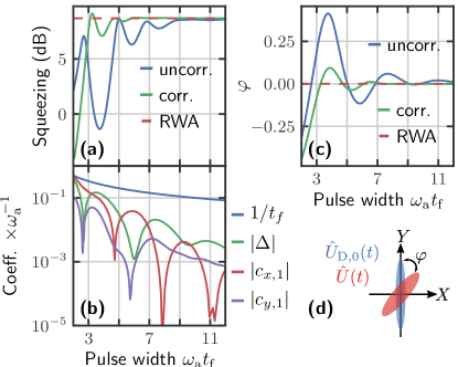
As one deviates from the weak driving limit, $\hat{V}_{\mathrm{D}}(t)$ cannot be neglected anymore. The generated dynamics becomes then more complex with the counter-rotating terms changing the direction along which the squeezing is generated as well as degrading the final degree of squeezing [see Fig. 3 (d)].

To mitigate the effects of $\hat{V}_{\mathrm{D}}(t)$ [see Eq. (56)], we consider a control Hamiltonian that corresponds to just changing the initial form of the parametric modulation. This leads to the correction Hamiltonian

$$\hat{W}_{\mathrm{PDC}}(t)=\sum\limits_{n} \left[g_{x}^{(n)}(t)\cos(\omega_{\mathrm{d}}t)+g_{y}^{(n)}(t)\sin(\omega_{\mathrm{d}}t)\right]$$ (58)

$$\times\left(\hat{a}+\hat{a}^{\dagger}\right)^{2}.$$

Furthermore, we are at liberty to drive the PDC at a frequency that is detuned from that of mode $\hat{a}$,

$$\frac{\omega_{\mathrm{a}}}{2}-\omega_{\mathrm{d}}=\Delta,$$ (59)

with $\Delta=\sum_{n}\Delta^{(n)}$ a static detuning.

Following the general procedure introduced in Sec. II (see Appendix E.2), we can easily determine $\Delta^{(n)}$, $g_{x}^{(n)}(t)$ and $g_{y}^{(n)}(t)$. We stress that in this example we correct the unitary evolution generated by Eq. (53), which allows us to generate the ideal squeezing dynamics for any initial state. This is in contrast to optimizing the dynamics to get optimal squeezing of the vacuum state only.

In Fig. 3 (a), we plot the degree of squeezing $S$ as a function of the total evolution time $t_{\mathrm{f}}$ for the RWA (red trace), the uncorrected (blue trace), and the corrected (green trace) evolutions. The degree of squeezing is given by

$$S=-10\log\left[\left(\langle\hat{y}^{2}\rangle_{f}-\langle\hat{y}\rangle_{f}^{2}\right)/\left(\langle\hat{y}^{2}\rangle_{i}-\langle\hat{y}\rangle_{i}^{2}\right)\right]$$ (60)

where $\hat{y}=(\hat{a}-\hat{a}^{\dagger})/i\sqrt{2}$, and $\langle\hat{y}\rangle_{i,f}=\langle\psi_{i,f}|\hat{y}|\psi_{i,f}\rangle$ is the quantum average of the operator $\hat{y}$ with respect to the initial and final states, respectively. Here, the initial state is the vacuum state $|0\rangle$. The initial pulse envelope is given by

$$f_{\mathrm{D}}(t)=\frac{1}{t_{\mathrm{f}}}\left[1-\cos\left(\frac{2\pi t}{t_{\mathrm{f}}}\right)\right].$$ (61)

Within the RWA the degree of squeezing is independent of the pulse width $t_{\mathrm{f}}$, since the squeezing depends just on $r(t_{\mathrm{f}})=c$. In the regime where the fast oscillating terms cannot be neglected, it is clear that the corrected evolution gives substantially better results (closer to the RWA evolution), specially for small values of $t_{\mathrm{f}}$. In Fig. 3 (c), we compute the deviation angle $\varphi$ in the phase space (with respect to the $y$-axis) where the maximum squeezing is obtained. Ideally, the maximum squeezing should be in the direction of the $y$-axis and $\varphi$ should be zero. With the correction Hamiltonian $\varphi$ is much closer to the ideal value. In Fig. 3 (b), we plot the coefficients of the correction Hamiltonian as a function of the total evolution time $t_{\mathrm{f}}$. As for the qubit case, we observe that the modified control fields can be seen as adding a small correction to the original control fields.

III.3 Transmon Qubit

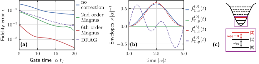
As a next example we consider the problem of realizing single-qubit gates with a transmon qubit Koch et al. (2007), where the logical qubit states are encoded in the two lowest energy states of an anharmonic oscillator with eigenstates $|n\rangle$ [see Fig. 4 (c)]. Since the oscillator is only weakly anharmonic, driving the $|0\rangle\leftrightarrow|1\rangle$ transition unavoidably leads to transitions to higher energy states outside of the computational subspace (leakage). Several strategies have been put forward to suppress leakage while implementing a gate, with perhaps the most well-known approach being DRAG (Derivative Removal by Adiabatic Gate) Motzoi et al. (2009); Gambetta et al. (2011). However, the correction predicted by DRAG cannot be fully implemented experimentally as it also requires one to drive the $|0\rangle\leftrightarrow|2\rangle$ transition. There is no charge matrix element connecting these states, hence it cannot be driven by an extra tone at the transition frequency. While neglecting this unrealizable control field is the simplest thing to do, this is a somewhat uncontrolled approximation; further, it has been demonstrated experimentally Chen et al. (2016) and theoretically Ribeiro et al. (2017) that this is indeed not the optimal approach. In the rest of this section, we demonstrate how our general strategy allows one to systematically find control sequences that are fully compatible with the constraints of the problem (i.e. no direct $|0\rangle\leftrightarrow|2\rangle$ drive, no time-dependent detuning), and also are highly efficient in suppressing both leakage and phase errors.

As in the original DRAG paper, we consider the three-level Hamiltonian

$$\hat{H}_{\mathrm{TLS}}(t)= \frac{\omega_{\mathrm{T}}}{2}\hat{\sigma}_{z}+\left(\frac{3\omega_{\mathrm{T}}}{2}+\alpha\right)|2\rangle\!\langle 2|$$ (62)

$$+f_{\mathrm{T}}(t)\cos(\omega_{\mathrm{d}}t)(\hat{\sigma}_{x}+\eta\hat{\nu}_{x,1})$$

as an approximation of the weakly anharmonic oscillator. Here, $\omega_{\mathrm{T}}$ is the frequency splitting between the energy levels $|0\rangle$ and $|1\rangle$ while the frequency splitting between $|1\rangle$ and $|2\rangle$ is given by $\omega_{\mathrm{T}}+\alpha$, where $\alpha$ is the anharmonicity. We have also defined the operators

$$\hat{\nu}_{x,12} =|1\rangle\!\langle 2|+|2\rangle\!\langle 1|,\ \hat{\nu}_{y,12}=i|2\rangle\!\langle 1|-i|1\rangle\!\langle 2|,$$ (63)

$$\hat{\nu}_{x,02} =|0\rangle\!\langle 2|+|2\rangle\!\langle 0|,\ \hat{\nu}_{y,02}=i|2\rangle\!\langle 0|-i|0\rangle\!\langle 2|,$$

which describe transitions between the logical qubit states and the leakage state $|2\rangle$. These operators together with the Pauli operators [see Eq. (33)] and the operator $|2\rangle\!\langle 2|$ form the operator basis for this problem [i.e. the operators $\hat{A}_{j}$ in Eq. (15)-(17)]. This set of eight operators (multiplied by the imaginary number $-i$) also form a Lie algebra with respect to the commutation operation, thus this set of eight operators can also be used to uniquely decompose the operators generated by the Magnus expansion.

The control pulse consists of a drive at frequency $\omega_{\mathrm{d}}$ and an envelope function $f_{\mathrm{T}}(t)$. As one can see from Eq. (62), driving the $|0\rangle\leftrightarrow|1\rangle$ transition also results in the $|1\rangle\leftrightarrow|2\rangle$ being driven with a relative strength given by $\eta$, which unavoidably generates leakage out the qubit subspace.

In a frame rotating with frequency $\omega_{\mathrm{d}}$, the Hamiltonian is given by $\hat{H}_{\mathrm{T}}(t)=\hat{H}_{\mathrm{T},0}(t)+\hat{V}_{\mathrm{T}}(t)$, where

$$\hat{H}_{\mathrm{T},0}(t)=\alpha|2\rangle\!\langle 2|+\frac{f_{\mathrm{T}}(t)}{2}\hat{\sigma}_{x},$$ (64)

and

$$\hat{V}_{\mathrm{T}}(t)=\eta\frac{f_{\mathrm{T}}(t)}{2}\hat{\nu}_{x,1}.$$ (65)

Here, we assume that the driving is on resonance with the $|0\rangle\leftrightarrow|1\rangle$ transition, i.e., $\omega_{\mathrm{T}}=\omega_{\mathrm{d}}$. The Hamiltonian $\hat{H}_{\mathrm{T},0}(t)$ gives us the desired interaction: it couples the levels $|0\rangle$ and $|1\rangle$, allowing one to perform unitary operations in the computational space, while leaving the level $|2\rangle$ isolated. The Hamiltonian $\hat{V}_{\mathrm{T}}(t)$ couples levels $|1\rangle$ and $|2\rangle$ leading to leakage out of the computational subspace. Note that we have neglected the terms oscillating at frequencies close to $2\omega_{\mathrm{d}}$ in Eqs. (64) and (65) (RWA).

Figure 4: Fast and high-fidelity single qubit gates with a transmon. (a) Average fidelity error for a Hadamard gate as a function of the gate time. The blue trace is calculated using the uncorrected Hamiltonian [see Eq. (62)]. The green trace is obtained for the 2nd order corrected Hamiltonian. The red trace is obtained for the 6th order corrected Hamiltonian. The purple trace is obtained using the DRAG correction. (b) Initial envelope functions (solid lines) and 6th order corrected envelope functions (dashed lines) for $\left|\alpha\right|t_{\mathrm{f}}=5$ [see Eq. (68)]. (c) Schematic energy level diagram of a transmon.

Given the constraints of the problem [see Eq. (64)], we want to find a correction that only involves modifying the drive envelope we use, and possibly changing the detuning in a static manner. We thus write the control Hamiltonian (in the rotating frame) as

$$\hat{W}_{\mathrm{TLS}}(t)= \sum\limits_{n}\left[g_{x}^{(n)}(t)\cos(\omega_{\mathrm{d}}t)+g_{y}^{(n)}(t)\sin(\omega_{\mathrm{d}}t)\right]$$ (66)

$$\times(\hat{\sigma}_{x}+\eta\hat{\nu}_{x,1}),$$

with $g_{x}^{(n)}(t)$ and $g_{y}^{(n)}(t)$ the unknown envelope functions. Furthermore, we allow the drive frequency to be detuned with respect to the base frequency of the transmon,

$$\omega_{\mathrm{T}}-\omega_{\mathrm{d}}=\Delta.$$ (67)

As for the envelope functions, the detuning is parametrized as a series: $\Delta=\sum_{n}\Delta^{(n)}$.

Within our framework, we would in principle need a total of eight free parameters to satisfy Eqs. (24), which determine the first-order correction; this is because there are eight operators in the basis. Taking into account that $|2\rangle$, which is outside the computational space, is of no interest to us, the equation associated to the operator $|2\rangle\!\langle 2|$ can be neglected. More generally, the equations originating from operators $\hat{A}_{j}$ that act strictly outside of the computational space do not need to be fulfilled, and one can simply neglect them to arrive at the relevant system of equations for the given order.

We are therefore left with seven equations to fulfill, and we need at least seven coefficients. However, we cannot select seven coefficients at random: we must retain enough harmonics to ensure that $g_{x}^{(n)}(t)$ and $g_{y}^{(n)}(t)$ have a bandwidth comparable to $\left|\alpha\right|$; this is needed to easily correct leakage transitions. This was also identified in an earlier work by Schutjens et al. Schutjens et al. (2013), which also aims at finding modified pulses to mitigate leakage errors in a transmon. Their strategy consists in suppressing the spectral weight associated to leakage transitions from the control fields. A systematic way of ensuring that the control fields have enough bandwidth is to keep more non-zero coefficients than necessary in their Fourier expansion. This choice leads to an underdetermined linear system of equations which can be solved using the Moore–Penrose pseudo-inverse Moore (1920); Bjerhammar (1951); Penrose (1955) (see Appendix F).

To show the performance of our strategy, we considered the situation where one wants to perform a Hadamard gate in the computational subspace. In Fig. 4 (a), we plot the average fidelity error as a function of the gate time $t_{\mathrm{f}}$. We compare the results obtained in the absence of any correction (blue trace) with the results for a 2nd order Magnus-based correction (green trace), a 6th order Magnus-based correction (red trace), and the DRAG correction (purple trace) Motzoi et al. (2009). The results show that the 6th order Magnus correction reduces the average fidelity error by more than four orders of magnitude for small $\left|\alpha t_{\mathrm{f}}\right|$, greatly outperforming the DRAG correction. In Fig. 4 (b) we compare the original and modified pulses for $|\alpha|t_{\mathrm{f}}=5$. For convenience we write the nth order modified pulse as

$$f_{\mathrm{\mathrm{T},mod}}(t)=f_{\mathrm{T},x}^{(n)}(t)\cos(\omega_{\mathrm{q}}t)+f_{\mathrm{T},y}^{(n)}(t)\sin(\omega_{\mathrm{q}}t),$$ (68)

where $f_{\mathrm{T},x}^{(n)}(t)=f_{\mathrm{T}}(t)+\sum_{k=1}^{n}g_{x}^{(k)}(t)$ and $f_{\mathrm{T},y}^{(n)}(t)=\sum_{k=1}^{n}g_{y}^{(k)}(t)$. The case $n=0$ corresponds to the original pulse, i.e., $f_{\mathrm{T},x}^{(0)}(t)=f_{\mathrm{T}}(t)$ and $f_{\mathrm{T},y}^{(0)}(t)=0$.

A legitimate concern at this point is related to the possibility of realizing the pulses obtained with the Magnus formalism, since arbitrary waveform generators (AWG) have bandwidth limitations. We remind the reader, however, that our method allows direct control over the bandwidth of the pulse through truncation of the Fourier series. If a stricter limitation over the bandwidth of the correction pulse is needed, one can make use of Lagrange multipliers to look for solutions of the linear system. As a rule of thumb, the minimum requirement of our method is that the AWG bandwidth should approximately be comparable to or larger than the anharmonicity $|\alpha|$.

III.4 SNAP Gates

We now turn to an example that combines both qubit and bosonic degrees of freedom. The general problem is to use a qubit coupled dispersively to a cavity to achieve control over the bosonic cavity mode. A method for doing this was recently proposed and implemented experimentally in a superconducting circuit QED architecture: the so-called SNAP gates (selective number-dependent arbitrary phase gates) combined with cavity displacements Heeres et al. (2015); Krastanov et al. (2015). Our goal will be to use our general method to accelerate SNAP gates without degrading their overall fidelity.

An optimal control approach based on GRAPE has been used to accelerate the manipulation of the bosonic cavity mode Heeres et al. (2017). There is, however, a major advantage in using SNAP gates in combination with cavity displacements: the SNAP gate can be made robust against qubit errors Reinhold et al. (2019), i.e., noise acting on the qubit will not affect the quantum state of the cavity.

As we will see, this problem involves an interesting technical subtlety. When introducing our general method in Sec. II, we stressed that it is crucial for the Hamiltonian $\hat{W}_{\mathrm{I}}(t)$ describing the modification of the control fields to have terms involving all of the basis operators $\hat{A}_{j}$ appearing in the Magnus expansion of the unitary evolution generated by the error-Hamiltonian $\hat{V}_{\mathrm{I}}(t)$. If this was not true, it would seemingly be impossible to correct errors proportional to these basis operators. Surprisingly, there are cases where this conclusion is overly pessimistic. In certain cases, one can still use a modified version of our Magnus-based strategy which uses an alternate method for finding an appropriate $\hat{W}(t)$. As we show below, correcting SNAP gates is an example of this kind of situation. The general price we pay is that now, to find an appropriate set of control corrections, we need to solve a nonlinear set of equations (instead of the linear equations in Eq. (26) that we used in all the previous examples).

The basic setup for SNAP gates involves a driven qubit that is dispersively coupled to a cavity mode. The Hamiltonian is $\hat{H}_{\mathrm{SNAP}}(t)=\hat{H}_{\mathrm{q}\mathrm{c}}+\hat{H}_{\mathrm{D}}(t)$, with

$$\hat{H}_{\mathrm{q}\mathrm{c}}=\frac{1}{2}\left(\omega_{\mathrm{q}}+\chi\hat{a}^{\dagger}\hat{a}\right)\hat{\sigma}_{z}+\omega_{\mathrm{c}}\hat{a}^{\dagger}\hat{a},$$ (69)

and

$$\hat{H}_{\mathrm{D}}(t)=[f_{x}(t)\cos(\omega_{\mathrm{d}}t)+f_{y}(t)\sin(\omega_{\mathrm{d}}t)]\hat{\sigma}_{x}.$$ (70)

The Pauli operators $\hat{\sigma}_{\alpha}$ act on the Hilbert space of the qubit and have been defined in Eq. (33). We also introduce the annihilation (creation) operator $\hat{a}$ ($\hat{a}^{\dagger}$) destroying (creating) an excitation of the oscillator. The qubit is driven by two independent pulses, $f_{x}(t)$ and $f_{y}(t)$, which couple both to $\hat{\sigma}_{x}$ with the same frequency $\omega_{\mathrm{d}}$ but with different phases.

In the interaction picture with respect to $\hat{H}_{\mathrm{q}\mathrm{c}}$, the Hamiltonian becomes

$$\hat{H}_{\mathrm{S}}(t) =\frac{1}{2}\sum_{n}\Big{(}f_{x}(t)\left[\cos(\delta\omega_{n}t)\hat{\sigma}_{x}-\sin(\delta\omega_{n}t)\hat{\sigma}_{y}\right]$$ (71)

$$-f_{y}(t)\left[\sin(\delta\omega_{n}t)\hat{\sigma}_{x}+\cos(\delta\omega_{n}t)\hat{\sigma}_{y}\right]\Big{)}|n\rangle\!\langle n|,$$

where $\delta\omega_{n}=\omega_{\mathrm{q}}+\chi n-\omega_{\mathrm{d}}$, $|n\rangle$ is a bosonic number state, and we have neglected fast oscillating terms. If the drive is now chosen to fulfil $\omega_{\mathrm{d}}=\omega_{\mathrm{q}}+\chi n_{0}$, so that the drive is resonant for a particular number-selected qubit transition, the Hamiltonian defined in Eq. (71) can be written as $\hat{H}_{\mathrm{S}}(t)=\hat{H}_{\mathrm{S},0}(t)+\hat{V}_{\mathrm{S}}(t)$. Here

$$\hat{H}_{\mathrm{S},0}(t)=\frac{1}{2}\Big{[}f_{x}(t)\hat{\sigma}_{x}-f_{y}(t)\hat{\sigma}_{y}\Big{]}|n_{0}\rangle\!\langle n_{0}|,$$ (72)

is the resonant part of the Hamiltonian defined in Eq. (71) and allows one to generate a unitary operation in the subspace spanned by $\{|g,n_{0}\rangle,|e,n_{0}\rangle\}$. In contrast

$$\hat{V}_{\mathrm{S}}(t)= \frac{1}{2}\sum_{n\neq n_{0}}\Big{(}f_{x}(t)\left[\cos(\delta\omega_{n}t)\hat{\sigma}_{x}-\sin(\delta\omega_{n}t)\hat{\sigma}_{y}\right]$$ (73)

$$-f_{y}(t)\left[\sin(\delta\omega_{n}t)\hat{\sigma}_{x}+\cos(\delta\omega_{n}t)\hat{\sigma}_{y}\right]\Big{)}|n\rangle\!\langle n|$$

is the non-resonant part of Eq. (71). This error Hamiltonian is responsible for the unwanted dynamics in the subspace spanned by $\{|g,n\rangle,|e,n\rangle\}$, for $n\neq n_{0}$. While in principle the effects of $\hat{V}_{\mathrm{S}}(t)$ on the dynamics cannot be avoided, they are minimal in the weak-driving regime where $f_{x}(t),f_{y}(t)\ll\chi$. In this limit, we can use $\hat{H}_{\mathrm{S},0}(t)$ to generate a dynamics that imprints a phase on $|n_{0}\rangle$ while leaving all other states $|n\rangle$ ($n\neq n_{0}$) unchanged. Our general goal will be to relax this weak-driving constraint, allowing for a faster overall gate.

For concreteness, we assume that the qubit is initially in the state $|g\rangle$ and the driving pulses $f_{x}(t)$ and $f_{y}(t)$ are chosen such that the qubit undergoes a cyclic evolution, i.e., the trajectory on the Bloch sphere encloses a finite solid angle and at $t=t_{\mathrm{f}}$ the state of the qubit is back to $|g\rangle$. This leads to the accumulation of a Berry phase $\gamma$ at $t=t_{\mathrm{f}}$ for the qubit which conditioned on the state of the cavity being $|n_{0}\rangle$. In other words,

$$\hat{U}_{\mathrm{S},0}(t_{\mathrm{f}})|g,n\rangle=\begin{cases}e^{i\gamma}|g,n\rangle&\text{if }n=n_{0},\\ |g,n\rangle&\text{if }n\neq n_{0},\end{cases}$$ (74)

where $\hat{U}_{\mathrm{S},0}(t_{\mathrm{f}})=\hat{T}\exp\left[-i\int_{0}^{t_{\mathrm{f}}}\mathop{}\!\mathrm{d}t\>\hat{H}_{\mathrm{S},0}(t)\right]$ is the unitary evolution generated by the ideal Hamiltonian in Eq. (72). This approach can be generalized so that the ideal evolution yields different qubit phase shifts for a set of different cavity photon numbers. One simply replaces the driving Hamiltonian [see Eq. (70)] by

$$\hat{H}_{\mathrm{d}}(t)=\sum_{n=0}^{N-1}[f_{x,n}(t)\cos(\omega_{\mathrm{d},n}t)+f_{y,n}(t)\sin(\omega_{\mathrm{d},n}t)]\hat{\sigma}_{x},$$ (75)

where $\omega_{\mathrm{d},n}=\omega_{\mathrm{q}}+\chi n$. The pulse envelopes $f_{x,n}(t)$ and $f_{y,n}(t)$ are chosen such that one gets the desired phase in the $n$th energy level.

Of course, the above ideal evolution requires that $f_{x,n}(t),f_{y,n}(t)\ll\chi$, constraining the overall speed of the gate. Without this assumption, the effects of the off-resonant error interaction given by the generalization of $\hat{V}_{\mathrm{S}}(t)$ [c.f. Eq. (73)] cannot be neglected, and will compromise the ideal SNAP gate evolution. Again, our goal is to mitigate these errors, allowing for faster gates.

In the following, we consider for simplicity the situation where one wants to imprint a phase on a single energy level of the oscillator. The extension to the more general situation where one imprints arbitrary phases in different levels is straightforward. We truncate the bosonic Hilbert space and work only within the subspace formed by the $N_{\mathrm{trunc}}$ first number states. This procedure is justified by the fact that SNAP gates are typically used to manipulate “kitten” states Heeres et al. (2015); Krastanov et al. (2015), which are themselves restricted to a truncated subspace of the original bosonic Hilbert space.

Figure 5: Accelerated SNAP gates. (a) Average fidelity error for a snap operation. A $\pi/2$ phase is imprinted in the cavity energy levels $|0\rangle$ and $|4\rangle$ simultaneously. The blue trace is calculated with the uncorrected Hamiltonian. The green trace is obtained with the 2nd order corrected Hamiltonian. The red trace is obtained with the 4th order corrected Hamiltonian. (b-c) Spectrum of the $x$ and $y$ components of the original pulse envelope and of the 4th order corrected pulse envelope for $\chi t_{\mathrm{f}}=50$. The uncorrected envelope has peaks at $\omega=0$ and $\omega=4\chi$. The corrected pulse has peaks close to $\omega=0,\chi,\ldots,9\chi$. This means that the corrected pulse simply undoes residual rotations caused by the non-resonant interaction in the different bosonic-number-state subspaces in order to bring the final state close to the target state.

As we did for the previous examples, we start by choosing a correction Hamiltonian $\hat{W}_{\mathrm{SNAP}}(t)$ that one can realize experimentally. Here, this corresponds to a modification of the qubit drive amplitudes:

$$\hat{W}_{\mathrm{SNAP}}(t)\!=\!\sum\limits_{n=0}^{N-1}[g_{x,n}(t)\cos(\omega_{\mathrm{d},n}t)+g_{y,n}(t)\sin(\omega_{\mathrm{d},n}t)]\hat{\sigma}_{x}\\$$ (76)

where $\omega_{\mathrm{d},n}=\omega_{\mathrm{q}}+\chi n$. Moving to the interaction picture with respect to $\hat{H}_{\mathrm{q}\mathrm{c}}$ [see Eq. (69)] and neglecting non-resonant terms, we obtain

$$\hat{W}_{\mathrm{S}}(t)=\frac{1}{2}\sum\limits_{n=0}^{N-1}[g_{x,n}(t)\hat{\sigma}_{x}-g_{y,n}(t)\hat{\sigma}_{y}]|n\rangle\!\langle n|.$$ (77)

In the interaction picture defined by $\hat{H}_{\mathrm{S},0}(t)$ [see Eq. (72)], we find that the form of the non-resonant error Hamiltonian is unchanged:

$$\hat{V}_{\mathrm{S},\mathrm{I}}(t)=\hat{V}_{\mathrm{S}}(t),$$ (78)

since $\hat{H}_{\mathrm{S},0}(t)$ commutes with $\hat{V}_{\mathrm{S}}(t)$; $\hat{H}_{\mathrm{S},0}(t)$ and $\hat{V}_{\mathrm{S}}(t)$ act on orthogonal subspaces. On the other hand, $\hat{W}_{\mathrm{S}}(t)$ acts on the whole Hilbert space, and is transformed when moving to the interaction picture. We find:

$$\hat{W}_{\mathrm{S},\mathrm{I}} (t)=\hat{U}_{\mathrm{S},0}^{\dagger}(t)\frac{1}{2}[g_{x,n_{0}}(t)\hat{\sigma}_{x}-g_{y,n_{0}}(t)\hat{\sigma}_{y}]|n_{0}\rangle\!\langle n_{0}|\hat{U}_{\mathrm{S},0}(t)$$ (79)

$$+\frac{1}{2}\sum\limits_{n=0}^{N-1}(1-\delta_{n,n_{0}})[g_{x,n}(t)\hat{\sigma}_{x}-g_{y,n}(t)\hat{\sigma}_{y}]|n\rangle\!\langle n|.$$

The first term of Eq. (79) acts on the $\{|g,n_{0}\rangle,|e,n_{0}\rangle\}$ subspace only and has terms proportional to all three Pauli matrices. While the explicit expression is too lengthy to be displayed here, it can be readily found using the group properties of the Pauli operators. The second term, which acts on the orthogonal subspace, has only terms proportional to $\hat{\sigma}_{x}|n\rangle\!\langle n|$ and $\hat{\sigma}_{y}|n\rangle\!\langle n|$. This means that the correction Hamiltonian in Eq. (76) cannot correct errors proportional to $\hat{\sigma}_{z}|n\rangle\!\langle n|$ (in the interaction picture) and which appear at 2nd order in the Magnus expansion of $\hat{V}_{\mathrm{S},\mathrm{I}}(t)$ [see Eq. (78)]. Unfortunately, an analysis of the Magnus expansion generated by Eq. (78) shows that these terms are by far the dominant source of errors which corrupt the ideal dynamics. We are left with no choice but to modify the general strategy of Sec. II that we have used successfully in all of the previous examples.

The naive thing to do would be to find an alternative control Hamiltonian that directly provides terms proportional to $\hat{\sigma}_{z}|n\rangle\!\langle n|$ in the interaction picture. However, in the lab frame this translates into a Hamiltonian with a dispersive coupling constant dependent on photon number $n$, i.e., we would need a term $\sum_{n}\chi_{n}|n\rangle\!\langle n|$ in Eq. (69). This is extremely difficult to achieve experimentally, hence we do not pursue this approach further.

A more promising approach is to use the fact that even though our original (constrained) correction Hamiltonian $\hat{W}_{\mathrm{S},\mathrm{I}}(t)$ is missing important terms, these can nonetheless be dynamically generated. In the same way that $\hat{V}_{\mathrm{S},\mathrm{I}}(t)$ generates problematic terms proportional to $\hat{\sigma}_{z}|n\rangle\!\langle n|$ at second order in the Magnus expansion, so can $\hat{W}_{\mathrm{S},\mathrm{I}}(t)$. Thus, we look for a correction Hamiltonian $\hat{W}^{(1)}(t)$ that cancels the sum of the first two terms of the Magnus expansion:

$$\hat{\Omega}_{1}^{(1)}(t_{\mathrm{f}})+\hat{\Omega}_{2}^{(1)}(t_{\mathrm{f}})=0.$$ (80)

This is in contrast of the general strategy in Sec. II, where we would just cancel the first term in the Magnus expansion.

We can use Eqs. (10) and (11) to write Eq. (80) in terms of integrals involving $\hat{V}_{\mathrm{S},\mathrm{I}}(t)$ [see Eq. (78)] and $\hat{W}_{\mathrm{S},\mathrm{I}}^{(1)}(t)$ [see Eq. (79) with $n=1$]. The explicit equation can be found in the Appendix G.1. Here, to be able to correct for the term proportional to $\hat{\sigma}_{z}|n\rangle\!\langle n|$, we cannot discard the higher order term generated by $\hat{W}_{\mathrm{S},\mathrm{I}}^{(1)}(t)$ in $\hat{\Omega}_{2}^{(1)}(t_{\mathrm{f}})$ (as the standard procedure prescribes). Once this is done, we proceed as usual: we expand the pulse envelopes $g_{x,n}(t)$ and $g_{y,n}(t)$ in a Fourier series, and we truncate the series keeping a sufficiently large number of free parameters . Following the strategy presented in Sec. II, we derive a system of equations for the free parameters, but instead of obtaining a linear system of equations we get a system of quadratic equations for the free parameters, since Eq. (80) is quadratic in $\hat{W}_{\mathrm{S},\mathrm{I}}^{(1)}(t)$. This system of equations can be solved numerically; see Appendix G.1, where we also show how one can find higher order corrections.

In the situation where one wishes to imprint non-zero phases to all energy levels of the truncated Hilbert space, one can actually solve the problem following the general (linear) strategy shown in Sec. II. In this case, since one is driving all frequencies resonantly, the ideal unitary $\hat{U}_{\mathrm{S},0}(t)$ acts on the whole truncated Hilbert space of the cavity. As a consequence, transforming the correction Hamiltonian $\hat{W}_{\mathrm{S}}(t)$ [see Eq. (77)] to the interaction picture will generate terms proportional to $\hat{\sigma}_{z}|n\rangle\!\langle n|$ for all values of $n$ (see Appendix G.2). We stress, however, that SNAP gates are most often used to manipulate logical qubit states encoded in a finite superposition of same parity bosonic number states Michael et al. (2016), e.g., $|0\rangle_{\mathrm{L}}=(|0\rangle+|4\rangle)/\sqrt{2}$ and $|1\rangle_{\mathrm{L}}=|2\rangle$. Accelerating SNAP gates that act on such logical qubit states requires one to use the strategy that cancels the sum of the first terms of the Magnus expansion [see Eq. (80)].

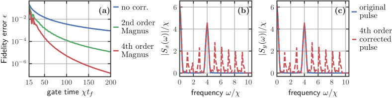
In Fig. 5 (a), we show the fidelity error when one tries to implement a fast SNAP gate that imprints a $\pi/2$ phase in the cavity energy levels $|0\rangle$ and $|4\rangle$ simultaneously. This is similar to implement a $Z$-gate for a logical qubit encoded in the states $|0\rangle_{\mathrm{L}}=(|0\rangle+|4\rangle)/\sqrt{2}$ and $|1\rangle_{\mathrm{L}}=|2\rangle$. The envelope functions for $n=0$ and $n=4$ are given by

$$f_{x,n}(t)=\begin{dcases}\frac{\pi}{2t_{\mathrm{f}}}\left[1-\cos\left(4\pi\frac{t}{t_{\mathrm{f}}}\right)\right],\quad&t<\frac{t_{\mathrm{f}}}{2},\\ 0,&t\geq\frac{t_{\mathrm{f}}}{2},\end{dcases}$$ (81)

and

$$f_{y,n}(t)=\begin{dcases}0,&t<\frac{t_{\mathrm{f}}}{2},\\ \frac{\pi}{2t_{\mathrm{f}}}\left[1-\cos\left(4\pi\frac{t}{t_{\mathrm{f}}}\right)\right],\quad&t\geq\frac{t_{\mathrm{f}}}{2}.\end{dcases}$$ (82)

For any other values of $n$, we have $f_{x,n}(t)=f_{y,n}(t)=0$. Here, we kept only ten energy levels for the cavity, i.e., the highest bosonic number state is $|10\rangle$, and the fidelity error was calculated using only the states within the truncated Hilbert space. We have plotted the fidelity as a function of gate time for the unmodified Hamiltonian (blue trace), for the second-order (green trace), and for the fourth order (red trace) modified Hamiltonians. Since we are only manipulating the cavity energy levels $|0\rangle$ and $|4\rangle$, we need to use the strategy that cancels the sum of the first terms of the Magnus expansion [see Eq. (80)]. The fourth order modified Hamiltonian achieves fidelity errors that are at least one order of magnitude smaller than the fidelity error of the original Hamiltonian. For larger values of $t_{\mathrm{f}}$ the difference can reach almost four orders of magnitude.

In Fig. 5 (b) and (c) we show the spectrum of the original and modified pulses for a gate time of $\chi t_{\mathrm{f}}=50$. The original pulse has only peaks located at $\omega=0$ and $\omega=4\chi$, since these are the frequencies of the levels being driven. The modified pulse, however, has peaks located at frequencies $\omega=0,\chi,2\chi,\ldots,9\chi$. This shows that the corrected pulse undoes residual rotations caused by the non-resonant interaction in the different bosonic number state subspaces in order to bring the final state close to the target state. It is important to note that the modified pulse corrects the dynamics only within the truncated Hilbert space. If the initial state of the cavity, i.e. the state before the SNAP operation is performed, is not confined to the truncated Hilbert space, the corrected pulse will not bring any improvement in terms of fidelity error, since the states lying outside the truncated Hilbert space will still be affected by the correction pulse.

IV Conclusion

We have developed a method that allows one to design high-fidelity control protocols which are always fully compatible with experimental constraints (available interactions and their tunability, bandwidth, etc.). At its core, our method uses the analytic solution of a simple control problem as a starting point to solve perturbatively a more complex problem, for which it is impossible to find closed-form analytic solutions. At the end of the day, the complex control problem is converted into solving a simple linear system of equations. We have applied our method to a range of problems, including the leakage problem in a transmon qubit and SNAP gates. We have shown how the control sequences predicted by our strategy allow one to substantially decrease the error of unitary operations while simultaneously speeding up the time require to complete the protocols. Finally, we note that the protocols generated by our method could be further improved by using them to seed a numerical optimal control algorithm.

V Acknowledgements

AC acknowledges partial support from the Center for Novel Pathways to Quantum Coherence in Materials, an Energy Frontier Research Center funded by the Department of Energy, Office of Science, Basic Energy Sciences.

Appendix A Nonresonant Perturbations

In Sec. II, where we introduced the general strategy to correct unitary evolution, we have taken as a starting point the Hamiltonian defined in Eq. (1), where the spurious error-Hamiltonian $\hat{V}(t)$ is multiplied by a small parameter $\epsilon$, such that $\hat{V}(t)$ can be considered as a perturbation. However, in all the examples discussed in the main text, the spurious error-Hamiltonian is not multiplied by a small parameter $\epsilon$, but by an oscillating function of time. Since integrating this oscillating function over a sufficiently long time interval leads to self-averaging, one can still view this class of error-Hamiltonians as a perturbation. The Magnus expansion provides a good way to formally show that.

Let us consider the generic oscillating Hamiltonian in the interaction picture,

$$\hat{V}_{\mathrm{I}}(t)=\frac{1}{t_{\mathrm{f}}}\left[e^{-i\omega_{\mathrm{V}}t}\hat{q}(t/t_{\mathrm{f}})+e^{i\omega_{\mathrm{V}}t}\hat{q}^{\dagger}(t/t_{\mathrm{f}})\right],$$ (83)

where $\omega_{\mathrm{V}}$ is the frequency at which the unwanted Hamiltonian $\hat{V}_{\mathrm{I}}(t)$ oscillates and $\hat{q}(t/t_{\mathrm{f}})$ is a bounded operator. Considering the Magnus expansion of the evolution operator $\hat{U}_{\mathrm{I}}(t)=\hat{T}\exp[-i\int_{0}^{t}\mathop{}\!\mathrm{d}t\>\hat{V}_{\mathrm{I}}(t)]$, where $\hat{T}$ is the time-ordering operator, we have to first order, at $t=t_{\mathrm{f}}$,

$$\hat{\Omega}_{1}(t_{\mathrm{f}}) =\int_{0}^{t_{\mathrm{f}}}\mathop{}\!\mathrm{d}t\>\hat{V}_{\mathrm{I}}(t)$$ (84)

$$=\frac{1}{\omega_{\mathrm{V}}t_{\mathrm{f}}}\bigl{[}ie^{-i\omega_{\mathrm{V}}t}\hat{q}(t/t_{\mathrm{f}})\bigl{|}_{0}^{t_{\mathrm{f}}}+H.c.\bigr{]}+\frac{1}{\omega_{\mathrm{V}}t_{\mathrm{f}}}\int_{0}^{t_{\mathrm{f}}}\mathop{}\!\mathrm{d}t\>\bigl{[}ie^{-i\omega_{\mathrm{V}}t}\frac{\mathrm{d}}{\mathop{}\!\mathrm{d}t}\hat{q}(t/t_{\mathrm{f}})+H.c.\bigr{]},$$ (85)

where Eq. (85) was obtained by integrating Eq. (84) by parts. One can perform the integration by parts repeatedly and obtain a series expansion for $\hat{\Omega}_{1}(t_{\mathrm{f}})$ in powers of $(\omega_{\mathrm{V}}t_{\mathrm{f}})^{-1}$. As one can see from Eq. (85), the leading order of $\hat{\Omega}_{1}(t_{\mathrm{f}})$ is $(\omega_{\mathrm{V}}t_{\mathrm{f}})^{-1}$. This suggests that $(\omega_{\mathrm{V}}t_{\mathrm{f}})^{-1}$ plays the role of the small parameter $\epsilon$. Taking this analogy one step further, one would naively assume that the leading order of $\hat{\Omega}_{n}(t_{\mathrm{f}})$ is $(\omega_{\mathrm{V}}t_{\mathrm{f}})^{-n}$, since this is the case when the error-Hamiltonian is proportional to $\epsilon$. This is, however, not true for oscillating Hamiltonians [see Eq. (83)]. To show that, let us calculate the second order term of the Magnus expansion,

$$\hat{\Omega}_{2}(t_{\mathrm{f}})=-\int_{0}^{t_{\mathrm{f}}}\mathop{}\!\mathrm{d}t_{1}\int_{0}^{t_{1}}\mathop{}\!\mathrm{d}t_{2}\>[\hat{V}_{\mathrm{I}}(t_{1}),\hat{V}_{\mathrm{I}}(t_{2})].$$ (86)

Substituting Eq. (83) in Eq. (86) and performing the integration in $t_{2}$ by parts, we obtain

$$\hat{\Omega}_{2}(t_{\mathrm{f}})=-\frac{1}{t_{\mathrm{f}}^{2}}\int_{0}^{t_{\mathrm{f}}}\mathop{}\!\mathrm{d}t_{1}\>\bigl{[}e^{-i\omega_{\mathrm{V}}t_{1}}\hat{q}(t_{1}/t_{\mathrm{f}})+H.c.,-\frac{e^{-i\omega_{\mathrm{V}}t_{2}}}{i\omega_{\mathrm{V}}}\hat{q}(t_{2}/t_{\mathrm{f}})\bigr{|}_{0}^{t_{1}}+H.c.\bigr{]}+\mathcal{O}[(\omega_{\mathrm{V}}t_{\mathrm{f}})^{-2}],$$ (87)

where we have omitted terms that are $\mathcal{O}[(\omega_{\mathrm{V}}t_{\mathrm{f}})^{-2}]$ and higher. Further simplifying Eq. (87), we find

$$\hat{\Omega}_{2}(t_{\mathrm{f}}) =-\frac{1}{t_{\mathrm{f}}^{2}}\int_{0}^{t_{\mathrm{f}}}\mathop{}\!\mathrm{d}t_{1}\>\Bigl{\{}\frac{i}{\omega_{\mathrm{V}}}\bigl{[}\hat{q}(t_{1}/t_{\mathrm{f}}),\hat{q}^{\dagger}(t_{1}/t_{\mathrm{f}})\bigr{]}+H.c.\Bigr{\}}+\mathcal{O}[(\omega_{\mathrm{V}}t_{\mathrm{f}})^{-2}]$$

$$=-\frac{1}{\omega_{\mathrm{V}}t_{\mathrm{f}}}\int_{0}^{1}\mathop{}\!\mathrm{d}x\>\bigl{\{}i\bigl{[}\hat{q}(x),\hat{q}^{\dagger}(x)\bigr{]}+H.c.\bigr{\}}+\mathcal{O}[(\omega_{\mathrm{V}}t_{\mathrm{f}})^{-2}],$$ (88)

which shows that $\hat{\Omega}_{2}(t_{\mathrm{f}})$ scales to leading order like $(\omega_{\mathrm{V}}t_{\mathrm{f}})^{-1}$.

Nevertheless, since we know the Magnus expansion converges, we must have that the leading order of $\hat{\Omega}_{n}(t)$ scales with higher powers of $(\omega_{\mathrm{V}}t_{\mathrm{f}})^{-1}$ for increasing $n$, but as we show above this dependence is not trivial. Numerical tests suggest that for nonresonant perturbations the leading order of $\hat{\Omega}_{j}^{(0)}(t_{\mathrm{f}})$ is given by

$$\hat{\Omega}_{j}^{(0)}(t_{\mathrm{f}})=\begin{dcases}0+\mathcal{O}\bigl{[}(\omega_{\mathrm{V}}t_{\mathrm{f}})^{-j/2}]&\text{if }j\text{ is even},\\ 0+\mathcal{O}\bigl{[}(\omega_{\mathrm{V}}t_{\mathrm{f}})^{-(j+1)/2}]&\text{if }j\text{ is odd}.\end{dcases}$$ (89)

Because of this property of nonresonant perturbations, one often needs to find the correction Hamiltonian $\hat{W}(t)$ up to second order to mitigate substantially the errors generated by $\hat{V}(t)$.

Appendix B The Magnus Expansion

In the main text we showed the expression only for the first two terms of the Magnus expansion. For the bosonic system, however, we have obtained a sixth order correction. The equations for the first four terms of the Magnus expansion are:

$$\partial_{t}\hat{\Omega}_{1}= -i\hat{H}_{\mathrm{I}},$$ (90)

$$\partial_{t}\hat{\Omega}_{2}= -\frac{1}{2}[\hat{\Omega}_{1},\partial_{t}\hat{\Omega}_{1}],$$ (91)

$$\partial_{t}\hat{\Omega}_{3}= -\frac{1}{2}[\hat{\Omega}_{2},\partial_{t}\hat{\Omega}_{1}]+\frac{1}{12}[\hat{\Omega}_{1},[\hat{\Omega}_{1},\partial_{t}\hat{\Omega}_{1}]],$$ (92)

$$\partial_{t}\hat{\Omega}_{4}= -\frac{1}{2}[\hat{\Omega}_{3},\partial_{t}\hat{\Omega}_{1}]+\frac{1}{12}[\hat{\Omega}_{2},[\hat{\Omega}_{1},\partial_{t}\hat{\Omega}_{1}]]+\frac{1}{12}[\hat{\Omega}_{1},[\hat{\Omega}_{2},\partial_{t}\hat{\Omega}_{1}]],$$ (93)

A generator for arbitrary order terms, which is convenient to obtain high order terms, can be found in the subsection 2.3 of Ref. Blanes et al. (2009).

When trying to calculate the Magnus expansion terms, one might be tempted to calculate the terms iteratively, i.e. firstly integrate eq. (90) to obtain $\hat{\Omega}_{1}$, then use this result to integrate Eq. (91) and obtain $\hat{\Omega}_{2}$, and so on. It is nonetheless much more efficient to treat all the terms that one intends to calculate as a system of differential equations and solve them simultaneously. In this work we solved the differential equations using the DifferentialEquations.jl package Rackauckas and Nie (2010) from the Julia programming language Bezanson et al. (2017).

Appendix C Arbitrary Order Corrections

A nth order correction, that generalizes Eq. (26) of the main text, must satisfy the following relation Ribeiro et al. (2017):

$$\int_{0}^{t_{\mathrm{f}}}\mathop{}\!\mathrm{d}t\ \hat{W}_{\mathrm{I}}^{(n)}(t)=-i\sum_{k=1}^{n}\hat{\Omega}_{k}^{(n-1)}(t_{\mathrm{f}}).$$ (94)

Since the set of operators $\{\hat{A}_{j}\}$ forms a basis and $\{-i\hat{A}_{j}\}$ generates a Lie algebra (see main text), we can write $\hat{\Omega}_{k}^{(l)}$ as a linear combination of the operators $\{\hat{A}_{j}\}$,

$$\hat{\Omega}_{k}^{(l)}(t)=\textstyle\sum\limits_{j}\Omega_{k,j}^{(l)}(t)\hat{A}_{j}.$$ (95)

Substituting Eqs. (22) of the main text and (95) in Eq. (94), we obtain

$$\int_{0}^{t_{\mathrm{f}}}\mathop{}\!\mathrm{d}t\ \tilde{w}_{j}^{(n)}(t)=-i\sum_{k=1}^{n}\Omega_{k,j}^{(n-1)}(t_{\mathrm{f}}).$$ (96)

The next steps are very similar to what was done for the first order correction. First, we expand $w_{j}^{(n)}(t)$ in a Fourier series [see Eq. (25) of the main text]. Since $\tilde{w}_{j}^{(n)}(t)=\sum_{l}w_{j}^{(n)}(t)a_{l,j}(t)$, we can substitute Eq. (25) of the main text in Eq. (96), and we obtain

$$M\>\mbox{\boldmath$x$}^{(n)}=\mbox{\boldmath$y$}^{(n)},$$ (97)

where $M$ is the same known $(N_{\mathrm{op}}\times N_{\mathrm{coeffs}})$ matrix obtained for $n=1$ [see Eq. (26) of the main text] and which encodes the dynamics of the ideal evolution generated $\hat{H}_{0}(t)$, $\mbox{\boldmath$x$}^{(n)}$ is the vector of the $N_{\mathrm{coeffs}}$ unknown Fourier coefficients $c_{lk}^{(n)}$ and $d_{lk}^{(n)}$ [see Eq. (25)], and $\mbox{\boldmath$y$}^{(n)}$ is the known vector of spurious elements we wish to average out. In the case where the summation in Eq. (25) runs from $0$ to $k_{\mathrm{max}}$ for all values of $j$, the explicit expressions for the elements of the matrix $M$ are given by Eq. (31). The elements of the vector $\mbox{\boldmath$x$}^{(n)}$ are

$$\mbox{\boldmath$x$}^{(n)}_{j}=\begin{dcases}c_{l,k}^{(n)}&\text{if }j\leq j_{0},\\ d_{l,k}^{(n)}&\text{if }j>j_{0}.\end{dcases}$$ (98)

Here $j_{0}=N_{\mathrm{op}}(k_{\mathrm{max}}+1)$, and $l$ and $k$ are given by the Eqs. (29) and (30) of the main text. The elements of $\mbox{\boldmath$y$}^{(n)}$ are given by

$$\mbox{\boldmath$y$}^{(n)}_{j}=-i\sum_{k=1}^{n}\Omega_{k,j}^{(n-1)}(t_{\mathrm{f}}).$$ (99)

Appendix D Strong Driving of a Two-Level System

D.1 Derivative-Based Correction

While discussing the problem of strong driving of a two-level system, we mention that other choices for $\hat{W}(t)$ were possible, but that they all require more resources to be implemented experimentally. In this appendix, we illustrate this by considering the derivate-based control method introduced in Ref. Ribeiro et al. (2017).

Let us first summarize the principle on which the derivate-based control method is built on. According to Eq. (14) of the main text, the first order correction term must satisfy

$$\int_{0}^{t_{\mathrm{f}}}\mathop{}\!\mathrm{d}t\ \hat{V}_{\mathrm{q},\mathrm{I}}(t)=-\int_{0}^{t_{\mathrm{f}}}\mathop{}\!\mathrm{d}t\ \hat{W}_{I}^{(1)}(t)$$ (100)

where $\hat{V}_{\mathrm{q},\mathrm{I}}(t)$ is given by Eq. (42) of the main text. Integrating the left hand side of Eq. (100) by parts, we find

$$\int_{0}^{t_{\mathrm{f}}}\mathop{}\!\mathrm{d}t\ \hat{V}_{\mathrm{q},\mathrm{I}}(t)= \frac{f_{\mathrm{q}}(t)}{4\omega_{\mathrm{d}}}\bigl{[}\sin(2\omega_{\mathrm{d}}t)\hat{\sigma}_{x}+\cos(2\omega_{\mathrm{d}}t)\cos{\theta}\hat{\sigma}_{y}-\cos(2\omega_{\mathrm{d}}t)\sin{\theta}\hat{\sigma}_{z}\bigr{]}\Bigl{|}_{0}^{t_{\mathrm{f}}}$$ (101)

$$-\frac{1}{4\omega_{\mathrm{d}}}\int_{0}^{t_{\mathrm{f}}}\mathop{}\!\mathrm{d}t\ \Bigl{\{}\dot{f}_{\mathrm{q}}(t)\sin(2\omega_{\mathrm{d}}t)\hat{\sigma}_{x}+\bigl{[}\dot{f}_{\mathrm{q}}(t)\cos{\theta}-f_{\mathrm{q}}^{2}(t)\sin{\theta}\bigr{]}\cos(2\omega_{\mathrm{d}}t)\hat{\sigma}_{y}$$

$$\qquad\qquad\qquad\quad+\bigl{[}\dot{f}_{\mathrm{q}}(t)\sin{\theta}+f_{\mathrm{q}}^{2}(t)\cos{\theta}\bigr{]}\cos(2\omega_{\mathrm{d}}t)\hat{\sigma}_{z}\Bigr{\}},$$

where we have omitted the explicit time dependence of $\theta$ for simplicity, i.e., $\theta=\theta(t)$. If the envelope function $f_{\mathrm{q}}(t)$ vanishes at $t=0$ and $t=t_{\mathrm{f}}$, Eq. (101) becomes

$$\int_{0}^{t_{\mathrm{f}}}\mathop{}\!\mathrm{d}t\ \hat{V}_{\mathrm{q},\mathrm{I}}(t)= 0-\frac{1}{4\omega_{\mathrm{d}}}\int_{0}^{t_{\mathrm{f}}}\mathop{}\!\mathrm{d}t\ \Bigl{\{}\dot{f}_{\mathrm{q}}(t)\sin(2\omega_{\mathrm{d}}t)\hat{\sigma}_{x}+\bigl{[}\dot{f}_{\mathrm{q}}(t)\cos{\theta}-f_{\mathrm{q}}^{2}(t)\sin{\theta}\bigr{]}\cos(2\omega_{\mathrm{d}}t)\hat{\sigma}_{y}$$ (102)

$$\qquad\qquad\qquad\quad+\bigl{[}\dot{f}_{\mathrm{q}}(t)\sin{\theta}+f_{\mathrm{q}}^{2}(t)\cos{\theta}\bigr{]}\cos(2\omega_{\mathrm{d}}t)\hat{\sigma}_{z}\Bigr{\}}.$$

Identifying Eq. (102) with Eq. (100), we find that a possible choice for $\hat{W}_{I}^{(1)}(t)$ is

$$\hat{W}_{\mathrm{I}}^{(1)}(t)=\tilde{w}_{1}^{(1)}(t)\hat{\sigma}_{x}+\tilde{w}_{2}^{(1)}(t)\hat{\sigma}_{y}+\tilde{w}_{3}^{(1)}(t)\hat{\sigma}_{z},$$ (103)

where

$$\tilde{w}_{1}^{(1)}(t) =\frac{1}{4\omega_{\mathrm{d}}}\dot{f}_{\mathrm{q}}(t)\sin(2\omega_{\mathrm{d}}t),$$ (104)

$$\tilde{w}_{2}^{(1)}(t) =\frac{1}{4\omega_{\mathrm{d}}}\bigl{[}\dot{f}(t)\cos{\theta}-f^{2}(t)\sin{\theta}\bigr{]}\cos(2\omega_{\mathrm{d}}t),$$ (105)

$$\tilde{w}_{3}^{(1)}(t) =\frac{1}{4\omega_{\mathrm{d}}}\bigl{[}\dot{f}(t)\sin{\theta}+f^{2}(t)\cos{\theta}\bigr{]}\cos(2\omega_{\mathrm{d}}t).$$ (106)

The second order control Hamiltonian $\hat{W}_{I}^{(2)}(t)$ can be found by considering the Magnus expansion associated to the unitary evolution generated by $\hat{H}_{\mathrm{mod,I}}^{(1)}(t)=\hat{V}_{\mathrm{I}}(t)+\hat{W}_{\mathrm{I}}^{(1)}(t)$. By construction, the first term of the Magnus expansion is given by

$$\hat{\Omega}_{1}^{(1)}(t)=-\frac{f_{\mathrm{q}}(t)}{4\omega_{\mathrm{d}}}\bigl{[}\sin(2\omega_{\mathrm{d}}t)\hat{\sigma}_{x}+\cos(2\omega_{\mathrm{d}}t)\cos{\theta}\hat{\sigma}_{y}-\cos(2\omega_{\mathrm{d}}t)\sin{\theta}\hat{\sigma}_{z}\bigr{]},$$ (107)

and vanishes at both $t=0$ and $t=t_{\mathrm{f}}$ because $f_{\mathrm{q}}(0)=f_{\mathrm{q}}(t_{\mathrm{f}})=0$.

According to Eq. (11) of the main text, the second term in the Magnus expansion is given by,

$$\Omega_{2}^{(1)}(t)-\Omega_{2}^{(1)}(0)=-\frac{i}{2}\int_{0}^{t}\mathop{}\!\mathrm{d}t_{1}\ \bigl{[}\hat{V}_{\mathrm{I}}(t_{1})+\hat{W}_{\mathrm{I}}^{(1)}(t_{1}),\hat{\Omega}_{1}^{(1)}(t_{1})\bigr{]}.$$ (108)

A natural choice for $\hat{W}_{I}^{(2)}(t)$ is then (see Eq. (12) of the main text)

$$\hat{W}_{I}^{(2)}(t)=-\frac{1}{2}\bigl{[}\hat{V}_{\mathrm{I}}(t)+\hat{W}_{I}^{(1)}(t),\hat{\Omega}_{1}(t)\bigr{]},$$ (109)

Transforming $\hat{W}_{I}^{(1)}(t)$ and $\hat{W}_{I}^{(2)}(t)$ back to the original frame, we obtain the correction Hamiltonian $\hat{W}(t)=\hat{W}^{(1)}(t)+\hat{W}^{(2)}(t)$. To implement this correction Hamiltonian, one would not only need to control in time the fields coupling to $\hat{\sigma}_{x}$ and $\hat{\sigma}_{z}$, but one would also need an extra time-dependent control field that couples to $\hat{\sigma}_{y}$.

D.2 Matrix Elements of $P_{\mathrm{q}}$

In this appendix, we give explicitly the matrix elements of the matrix $P_{\mathrm{q}}$ introduced in Eq. (50) of the main text when discussing the strong driving of a qubit. We have

$$P_{\mathrm{q},11} =\int_{0}^{t_{\mathrm{f}}}\mathop{}\!\mathrm{d}t\>[1-\cos(\omega_{1}t)]\cos^{2}(\omega_{\mathrm{d}}t),$$ (110)

$$P_{\mathrm{q},12} =\int_{0}^{t_{\mathrm{f}}}\mathop{}\!\mathrm{d}t\>[1-\cos(\omega_{1}t)]\sin(\omega_{\mathrm{d}}t)\cos(\omega_{\mathrm{d}}t),$$ (111)

$$P_{\mathrm{q},13} =0,$$ (112)

$$P_{\mathrm{q},21} =-\int_{0}^{t_{\mathrm{f}}}\mathop{}\!\mathrm{d}t\>[1-\cos(\omega_{1}t)]\sin(\omega_{\mathrm{d}}t)\cos(\omega_{\mathrm{d}}t)\cos{\theta},$$ (113)

$$P_{\mathrm{q},22} =-\int_{0}^{t_{\mathrm{f}}}\mathop{}\!\mathrm{d}t\>[1-\cos(\omega_{1}t)]\sin^{2}(\omega_{\mathrm{d}}t)\cos{\theta},$$ (114)

$$P_{\mathrm{q},23} =\int_{0}^{t_{\mathrm{f}}}\mathop{}\!\mathrm{d}t\>\sin{\theta},$$ (115)

$$P_{\mathrm{q},31} =\int_{0}^{t_{\mathrm{f}}}\mathop{}\!\mathrm{d}t\>[1-\cos(\omega_{1}t)]\sin(\omega_{\mathrm{d}}t)\cos(\omega_{\mathrm{d}}t)\sin{\theta},$$ (116)

$$P_{\mathrm{q},32} =\int_{0}^{t_{\mathrm{f}}}\mathop{}\!\mathrm{d}t\>[1-\cos(\omega_{1}t)]\sin^{2}(\omega_{\mathrm{d}}t)\sin{\theta},$$ (117)

$$P_{\mathrm{q},33} =\int_{0}^{t_{\mathrm{f}}}\mathop{}\!\mathrm{d}t\>\cos{\theta},$$ (118)

where once more we have omitted the explicit time dependence of $\theta$.

Appendix E Strong Driving of a Parametrically Driven Cavity

E.1 The Operators $\hat{\mu}_{x}$, $\hat{\mu}_{y}$, and $\hat{\mu}_{z}$

In this section, we give the commutation relations for the operators $\hat{\mu}_{x}$, $\hat{\mu}_{y}$, and $\hat{\mu}_{z}$ introduced in Eq. (54) of the main text when discussing the strong driving of a parametrically driven cavity. These operators behave as generators of the group SU$(1,1)$ and consequently generate the su$(1,1)$ Lie algebra, which one can readily verify by computing the commutation relations. We have

$$=2i\hat{\mu}_{z},$$ (119)

$$[\hat{\mu}_{x},\hat{\mu}_{z}] =2i\hat{\mu}_{y},$$

$$[\hat{\mu}_{z},\hat{\mu}_{y}] =2i\hat{\mu}_{x}.$$

Therefore these three operators are enough to fully characterize the dynamics of the parametrically driven cavity in spite of having an infinite Hilbert space.

E.2 Correction Hamiltonian

In this appendix we give some more details about the steps of the general method applied to the problem of strong driving of a parametrically driven cavity.

Following the general procedure described in the general theory (see Sec.II of the main text), we start by writing the full modified Hamiltonian in the frame rotating at the drive frequency $\omega_{\mathrm{d}}$:

$$\hat{H}_{\mathrm{\mathrm{D},mod}}(t)=\hat{H}_{\mathrm{D},0}(t)+\hat{V}_{\mathrm{D}}(t)+\sum_{n}\hat{W}_{\mathrm{D}}^{(n)}(t),$$ (120)

where $\hat{H}_{\mathrm{D},0}(t)$ and $\hat{V}_{\mathrm{D}}(t)$ are, respectively, given by Eq. (55) and Eq. (56) of the main text, and

$$\hat{W}_{\mathrm{D}}^{(n)}(t)=2g^{(n)}(t)\cos(\omega_{\mathrm{d}}t)\hat{\mu}_{x}+2g^{(n)}(t)\sin(\omega_{\mathrm{d}}t)\hat{\mu}_{y}+[\Delta^{(n)}+2g^{(n)}(t)]\hat{\mu}_{z}.$$ (121)

Once more, we stress that the final detuning is given by $\Delta=\sum_{n}\Delta^{(n)}$.

Following our recipe, we now move to the interaction picture with respect to $\hat{H}_{\mathrm{D},0}(t)$. The Hamiltonian $\hat{V}_{\mathrm{D}}(t)$ is then given by

$$\hat{V}_{\mathrm{D},\mathrm{I}}(t)=\tilde{v}_{\mathrm{D},x}(t)\hat{\mu}_{x}+\tilde{v}_{\mathrm{D},y}(t)\hat{\mu}_{y}+\tilde{v}_{\mathrm{D},z}(t)\hat{\mu}_{z},$$ (122)

where

$$\tilde{v}_{\mathrm{D},x}(t) =f_{\mathrm{D}}(t)[\sin(2\omega_{\mathrm{d}}t)\cosh(2r)+2\sin(\omega_{\mathrm{d}}t)\sinh(2r)],$$ (123)

$$\tilde{v}_{\mathrm{D},y}(t) =-f_{\mathrm{D}}(t)\cos(2\omega_{\mathrm{d}}t),$$

$$\tilde{v}_{\mathrm{D},y}(t) =f_{\mathrm{D}}(t)[\sin(2\omega_{\mathrm{d}}t)\sinh(2r)+2\sin(\omega_{\mathrm{d}}t)\cosh(2r)].$$

Similarly, we find that the correction Hamiltonian in the interaction picture is given by

$$\hat{W}_{\mathrm{D},\mathrm{I}}^{(n)}(t)=\tilde{w}_{\mathrm{D},x}^{(n)}(t)\hat{\mu}_{x}+\tilde{w}_{\mathrm{D},y}^{(n)}(t)\hat{\mu}_{y}+\tilde{w}_{\mathrm{D},z}^{(n)}(t)\hat{\mu}_{z},$$ (124)

where

$$\tilde{w}_{\mathrm{D},x}^{(n)}(t) =2g^{(n)}(t)\cos(\omega_{\mathrm{d}}t)\cosh(2r)+[\Delta^{(n)}+2g^{(n)}(t)]\sinh(2r),$$ (125)

$$\tilde{w}_{\mathrm{D},y}^{(n)}(t) =2g^{(n)}(t)\sin(\omega_{\mathrm{d}}t),$$

$$\tilde{w}_{\mathrm{D},z}^{(n)}(t) =2g^{(n)}(t)\cos(\omega_{\mathrm{d}}t)\sinh(2r)+[\Delta^{(n)}+2g^{(n)}(t)]\cosh(2r).$$

For simplicity we have omitted the explicit time dependence of $r$, i.e., $r=r(t)$ [see Eq. (57) of the main text], in Eqs. (123) and (125).

E.3 The Linear System of Equations

In this section we give explicitly the matrix elements of $P_{\mathrm{D}}$. As explained in Sec. III.1, the matrix $P_{\mathrm{D}}$ is analog to the matrix $M$ introduced in Eq. (26) of the main text and encodes the dynamics of the ideal evolution generated by $\hat{H}_{\mathrm{D},0}(t)$ (see Eq. (55) of the man text). The difference comes from our choice of expanding in a Fourier series the unknown envelope functions $g_{\alpha}^{(n)}(t)$ ($\alpha=x,y$, see Eq. (58) of the main text) and the static detuning $\Delta^{(n)}$ instead of the functions $\tilde{w}_{\mathrm{D},\alpha}(t)$ [$\alpha=x,y,z$, see Eq. (125)]. Within this framework, the system of linear equations that allows one to determine the coefficients defining the nth order control correction is

$$P_{\mathrm{D}}\mbox{\boldmath$x$}_{\mathrm{D}}^{(n)}=\mbox{\boldmath$y$}_{\mathrm{D}}^{(n)},$$ (126)

where $\mbox{\boldmath$x$}_{\mathrm{D}}^{(n)}=\{c_{x,n}^{(1)},c_{y,n}^{(1)},\Delta^{(n)}\}^{T}$ is the vector of unknown coefficients and $\mbox{\boldmath$y$}_{\mathrm{D}}^{(n)}$ is the vector of spurious error-Hamiltonian elements. To first order we have $\mbox{\boldmath$y$}_{\mathrm{D}}^{(1)}=-\int_{0}^{t_{\mathrm{f}}}\mathop{}\!\mathrm{d}t\{\tilde{v}_{\mathrm{D},x}(t),\tilde{v}_{\mathrm{D},y}(t),\tilde{v}_{\mathrm{D},z}(t)\}^{T}$, with $\tilde{v}_{\mathrm{D},\alpha}(t)$ ($\alpha=x,y,z$) given in Eq. (123).

Finally, the matrix elements of $P_{\mathrm{D}}$ are

$$P_{\mathrm{D},11} =\int_{0}^{t_{\mathrm{f}}}\mathop{}\!\mathrm{d}t\>[1-\cos(\omega_{1}t)]\bigl{\{}[1+\cos(4t)]\cosh[2r]+2\cos(2t)\sinh[2r]\bigr{\}},$$ (127)

$$P_{\mathrm{D},12} =\int_{0}^{t_{\mathrm{f}}}\mathop{}\!\mathrm{d}t\>[1-\cos(\omega_{1}t)]\bigl{\{}\sin(4t)\cosh[2r]+2\sin(2t)\sinh[2r]\bigr{\}},$$ (128)

$$P_{\mathrm{D},13} =\int_{0}^{t_{\mathrm{f}}}\mathop{}\!\mathrm{d}t\sinh[2r],$$ (129)

$$P_{\mathrm{D},21} =-\int_{0}^{t_{\mathrm{f}}}\mathop{}\!\mathrm{d}t\>[1-\cos(\omega_{1}t)]\sin(4t),$$ (130)

$$P_{\mathrm{D},22} =-\int_{0}^{t_{\mathrm{f}}}\mathop{}\!\mathrm{d}t\>[1-\cos(\omega_{1}t)][1-\cos(4t)],$$ (131)

$$P_{\mathrm{D},23} =0,$$ (132)

$$P_{\mathrm{D},31} =\int_{0}^{t_{\mathrm{f}}}\mathop{}\!\mathrm{d}t\>[1-\cos(\omega_{1}t)]\bigl{\{}[1+\cos(4t)]\sinh[2r]+2\cos(2t)\cosh[2r]\bigr{\}},$$ (133)

$$P_{\mathrm{D},32} =\int_{0}^{t_{\mathrm{f}}}\mathop{}\!\mathrm{d}t\>[1-\cos(\omega_{1}t)]\bigl{\{}\sin(4t)\sinh[2r]+2\sin(2t)\cosh[2r]\bigr{\}},$$ (134)

$$P_{\mathrm{D},33} =\int_{0}^{t_{\mathrm{f}}}\mathop{}\!\mathrm{d}t\>\cosh[2r],$$ (135)

where $\omega_{1}=2\pi/t_{\mathrm{f}}$ and once more we have omitted the explicit time dependence of $r$.

Appendix F Transmon Qubit

F.1 Interaction Picture

In this appendix we show some steps of the general method applied to the transmon qubit that were omitted in the main text for brevity.

We first write the full modified Hamiltonian in a frame rotating with the drive frequency:

$$\hat{H}_{\mathrm{T},\mathrm{mod}}(t)=\hat{H}_{\mathrm{T},0}(t)+\hat{V}_{\mathrm{T}}(t)+\sum\limits_{n}\hat{W}_{\mathrm{T}}^{(n)}(t),$$ (136)

where $\hat{H}_{\mathrm{T},0}(t)$ is given by Eq. (64), $\hat{V}_{\mathrm{T}}(t)$ is given by Eq. (65), and

$$\hat{W}_{\mathrm{T}}^{(n)}=\frac{1}{2}\Delta^{(n)}\bigl{(}\hat{\sigma}_{z}+3|2\rangle\!\langle 2|\bigr{)}+\frac{1}{2}g_{x}^{(n)}(t)\left(\hat{\sigma}_{x}+\eta\hat{\nu}_{x,12}\right)+\frac{1}{2}g_{y}^{(n)}(t)\left(-\hat{\sigma}_{y}+\eta\hat{\nu}_{y,12}\right).$$ (137)

As we previously did for the two-level system (see Sec. III.1) and the DPA (see Sec. III.2), we use the detuning as yet another free parameter in the control Hamiltonian.

Before we move to the interaction picture with respect to $\hat{H}_{\mathrm{T},0}(t)$, let us adopt, for convenience, the following notation:

$$\hat{\lambda}_{1},\hat{\lambda}_{2},\hat{\lambda}_{3}=\hat{\sigma}_{x},\hat{\sigma}_{y},\hat{\sigma}_{z};$$ (138)

$$\hat{\lambda}_{4},\hat{\lambda}_{5},\hat{\lambda}_{6},\hat{\lambda}_{7}=\hat{\nu}_{x,12},\hat{\nu}_{y,12},\hat{\nu}_{x,02},\hat{\nu}_{y,02};$$

$$\hat{\lambda}_{8}=|2\rangle\!\langle 2|.$$

Moving to the interaction picture with respect to $\hat{H}_{\mathrm{T},0}(t)$, the Hamiltonian $\hat{V}_{\mathrm{T}}(t)$ is given by

$$\hat{V}_{\mathrm{T},\mathrm{I}}(t)=\tilde{v}_{\mathrm{T},1}(t)\hat{\lambda}_{1}+\tilde{v}_{\mathrm{T},2}(t)\hat{\lambda}_{2}+\tilde{v}_{\mathrm{T},3}(t)\hat{\lambda}_{3}+\tilde{v}_{\mathrm{T},4}(t)\hat{\lambda}_{4}+\tilde{v}_{\mathrm{T},5}(t)\hat{\lambda}_{5}+\tilde{v}_{\mathrm{T},6}(t)\hat{\lambda}_{6}+\tilde{v}_{\mathrm{T},7}(t)\hat{\lambda}_{7}+\tilde{v}_{\mathrm{T},8}(t)\hat{\lambda}_{8},$$ (139)

where

$$\tilde{v}_{\mathrm{T},1}(t) =\tilde{v}_{\mathrm{T},2}(t)=\tilde{v}_{\mathrm{T},3}(t)=0,$$ (140)

$$\tilde{v}_{\mathrm{T},4}(t) =\frac{\eta}{2}f_{\mathrm{T}}(t)\cos(\theta/2)\cos(\alpha t),$$

$$\tilde{v}_{\mathrm{T},5}(t) =\frac{\eta}{2}f_{\mathrm{T}}(t)\cos(\theta/2)\sin(\alpha t),$$

$$\tilde{v}_{\mathrm{T},6}(t) =\frac{\eta}{2}f_{\mathrm{T}}(t)\sin(\theta/2)\sin(\alpha t),$$

$$\tilde{v}_{\mathrm{T},7}(t) =-\frac{\eta}{2}f_{\mathrm{T}}(t)\sin(\theta/2)\cos(\alpha t),$$

$$\tilde{v}_{\mathrm{T},8}(t) =0,$$

where for simplicity we have omitted the explicit time dependence of $\theta$, i.e.,

$$\theta(t)=\int_{0}^{t}\mathop{}\!\mathrm{d}t_{1}f_{\mathrm{T}}(t_{1}).$$ (141)

Proceeding similarly we find

$$\hat{W}_{\mathrm{T},\mathrm{I}}^{(n)}(t)=\tilde{w}_{\mathrm{T},1}^{(n)}(t)\hat{\lambda}_{1}+\tilde{w}_{\mathrm{T},2}^{(n)}(t)\hat{\lambda}_{2}+\tilde{w}_{\mathrm{T},3}^{(n)}(t)\hat{\lambda}_{3}+\tilde{w}_{\mathrm{T},4}^{(n)}(t)\hat{\lambda}_{4}+\tilde{w}_{\mathrm{T},5}^{(n)}(t)\hat{\lambda}_{5}+\tilde{w}_{\mathrm{T},6}^{(n)}(t)\hat{\lambda}_{6}+\tilde{w}_{\mathrm{T},7}^{(n)}(t)\hat{\lambda}_{7}+\tilde{w}_{\mathrm{T},8}^{(n)}(t)\hat{\lambda}_{8}$$ (142)

where

$$\tilde{w}_{\mathrm{T},1}^{(n)}(t) =\frac{1}{2}g_{x}^{(n)}(t),$$ (143)

$$\tilde{w}_{\mathrm{T},2}^{(n)}(t) =\frac{1}{2}g_{y}^{(n)}(t)\cos{\theta}+\frac{1}{2}\Delta^{(n)}\sin{\theta},$$

$$\tilde{w}_{\mathrm{T},3}^{(n)}(t) =-\frac{1}{2}g_{y}^{(n)}(t)\sin{\theta}+\frac{1}{2}\Delta^{(n)}\cos{\theta},$$

$$\tilde{w}_{\mathrm{T},4}^{(n)}(t) =\frac{\eta}{2}\left[g_{x}^{(n)}(t)\cos(\alpha t)\cos(\theta/2)-g_{y}^{(n)}(t)\sin(\alpha t)\cos(\theta/2)\right],$$

$$\tilde{w}_{\mathrm{T},5}^{(n)}(t) =\frac{\eta}{2}\left[g_{x}^{(n)}(t)\sin(\alpha t)\cos(\theta/2)+g_{y}^{(n)}(t)\cos(\alpha t)\cos(\theta/2)\right],$$

$$\tilde{w}_{\mathrm{T},6}^{(n)}(t) =\frac{\eta}{2}\left[g_{x}^{(n)}(t)\sin(\alpha t)\sin(\theta/2)+g_{y}^{(n)}(t)\cos(\alpha t)\sin(\theta/2)\right],$$

$$\tilde{w}_{\mathrm{T},7}^{(n)}(t) =\frac{\eta}{2}\left[-g_{x}^{(n)}(t)\cos(\alpha t)\sin(\theta/2)+g_{y}^{(n)}(t)\sin(\alpha t)\sin(\theta/2)\right],$$

$$\tilde{w}_{\mathrm{T},8}^{(n)}(t) =\frac{3}{2}\Delta^{(n)}.$$

It is convenient to use the Gell-Mann $\hat{\lambda}$ operators to calculate commutators. The Gell-Mann $\hat{\lambda}$ operators are given by Eq. (138), except for $\hat{\lambda}_{8}$, which is given by

$$\hat{\lambda}_{8}=(|0\rangle\!\langle 0|+|1\rangle\!\langle 1|-2|2\rangle\!\langle 2|)/\sqrt{3}$$ (144)

The Gell-Mann operators satisfy the following commutation relations:

$$[\hat{\lambda}_{a},\hat{\lambda}_{b}]=2i\textstyle\sum\limits_{c}f^{abc}\hat{\lambda}_{c},$$ (145)

where the structure constants $f^{abc}$ are completely antisymmetric in the three indices, and are given by

$$f^{123}=1,\ f^{147}=f^{165}=f^{246}=f^{257}=f^{345}=f^{376}=\frac{1}{2},\ f^{458}=f^{678}=\frac{\sqrt{3}}{2}.$$ (146)

The commutation relations of the Gell-Mann matrices are very convenient, specially when evaluating the Magnus expansion for this problem.

F.2 Choice of Free Parameters

In the main text we showed that one has seven equations to fulfill for the transmon qubit problem, and this requires at least seven free parameters. We also commented that it is important that the envelope functions $g_{x}^{(n)}(t)$ and $g_{y}^{(n)}(t)$ of the correction Hamiltonian (see Eq. (66) of the main text) have a bandwidth comparable to $\left|\alpha\right|$, so that one can access transitions between the levels $|1\rangle$ and $|2\rangle$. This becomes more clear if one considers the expressions of $\tilde{w}_{\mathrm{T},j}^{(n)}(t)$ in Eqs. (143). One can see that $\tilde{w}_{\mathrm{T},j}^{(n)}(t)$ oscillates with frequency $\left|\alpha\right|$ for $j=4,\ldots,7$, while $\tilde{w}_{\mathrm{T},j}^{(n)}(t)$ is a slowly varying function for other values of $j$. Since the effect of the correction Hamiltonian on the dynamics at $t=t_{\mathrm{f}}$ is given by the integral of $\hat{W}_{\mathrm{T},\mathrm{I}}(t)$, the terms proportional to $\hat{\lambda}_{4},\ldots,\hat{\lambda}_{7}$ average out unless $g^{(n)}(t)$ has a bandwidth comparable to $\left|\alpha\right|$. As a consequence $g_{x}^{(n)}(t)$ and $g_{y}^{(n)}(t)$ must have a bandwidth comparable to $\left|\alpha\right|$.

Practically, this means that the envelope functions $g_{x}^{(n)}(t)$ and $g_{y}^{(n)}(t)$ associated to the correction Hamiltonian (see Eq. (66) of the main text) need to have a certain number of non-zero coefficients such that the condition on the bandwidth can be satisfied. A systematic way of determining which coefficients are non-zero is to choose the coefficients of the harmonics between $k=1$ and $k\simeq\left|\alpha\right|t_{\mathrm{f}}/2\pi$ in the Fourier expansion of the envelopes to be non-zero and set all the other coefficients to zero. Furthermore, assuming that the detuning is time-independent, all coefficients of its Fourier series except $c_{z,0}$ are zero. This typically gives us more than seven free coefficients in total, and we end up with an underdetermined system of linear equations.

As mentioned in the main text, we can use the Moore–Penrose pseudo-inverse Moore (1920); Bjerhammar (1951); Penrose (1955) to solve this underdetermined system of linear equations. Importantly, the pseudo-inverse always exists, which guarantees that the linear system always has a solution, and the pseudo-inverse also enforces that the solution has the smallest possible norm, which results in having only a fraction of the free coefficients to actually be non-zero.

Appendix G SNAP Gates

G.1 Correction Hamiltonian

As discussed in the main text, the correction Hamiltonian for SNAP gates (see Eq. (76) of the main text) does not allow one to correct terms proportional to $\hat{\sigma}_{z}|n\rangle\!\langle n|$ using the general strategy presented in Sec. II. As we argue in the main text, the most important source of errors are precisely those originating from terms in the error-Hamiltonian proportional to $\hat{\sigma}_{z}|n\rangle\!\langle n|$. This makes it necessary to find another strategy to correct those errors.

A correction Hamiltonian with terms proportional to $\hat{\sigma}_{z}|n\rangle\!\langle n|$ in the rotating frame is out of question, since it would require a dispersive coupling constant dependent on $n$. We must, therefore, abandon the general strategy used so far and look for an alternative approach.

Let us write explicitly the Magnus expansion, up to the second order, of the evolution operator associated to the modified Hamiltonian $\hat{H}_{mod,\mathrm{I}}^{(1)}(t)=\hat{V}_{\mathrm{S},\mathrm{I}}(t)+\hat{W}_{\mathrm{S},\mathrm{I}}^{(1)}(t)$. We have

$$\hat{\Omega}_{1}^{(1)}(t_{\mathrm{f}})+\hat{\Omega}_{2}^{(1)}(t_{\mathrm{f}})= \hat{\Omega}_{1}^{(0)}(t_{\mathrm{f}})+\hat{\Omega}_{2}^{(0)}(t_{\mathrm{f}})-i\int_{0}^{t_{\mathrm{f}}}\mathop{}\!\mathrm{d}t_{1}\hat{W}_{\mathrm{S},\mathrm{I}}^{(1)}(t_{1})$$ (147)

$$-\frac{1}{2}\int_{0}^{t_{\mathrm{f}}}\mathop{}\!\mathrm{d}t_{1}\int_{0}^{t_{1}}\mathop{}\!\mathrm{d}t_{2}\>\Bigl{\{}\bigl{[}\hat{V}_{\mathrm{S},\mathrm{I}}(t_{1}),\hat{W}_{\mathrm{S},\mathrm{I}}^{(1)}(t_{2})\bigl{]}+\bigl{[}\hat{W}_{\mathrm{S},\mathrm{I}}^{(1)}(t_{1}),\hat{V}_{\mathrm{S},\mathrm{I}}(t_{2})\bigr{]}+\bigl{[}\hat{W}_{\mathrm{S},\mathrm{I}}^{(1)}(t_{1}),\hat{W}_{\mathrm{S},\mathrm{I}}^{(1)}(t_{2})\bigr{]}\Bigr{\}}$$

In the general strategy presented in Sec. II, we neglect the term originating from the double integral with the argument that it is a high order term in the perturbative series. However, if one calculates the commutators $[\hat{H}_{\mathrm{mod},\mathrm{I}}^{(0)}(t_{1}),\hat{W}_{\mathrm{S},\mathrm{I}}^{(1)}(t_{2})]$ and $[\hat{W}_{\mathrm{S},\mathrm{I}}^{(1)}(t_{1}),\hat{W}_{\mathrm{S},\mathrm{I}}^{(1)}(t_{2})]$ (cf. Eqs. (78) and (79) of the main text), one finds terms proportional to $\hat{\sigma}_{z}|n\rangle\!\langle n|$. This gives us a path forward to find a correction Hamiltonian: we will keep the higher order term originating from the double integral in Eq. (147) and try to find a correction Hamiltonian $\hat{W}_{\mathrm{S},\mathrm{I}}^{(1)}(t)$ that guarantees that $\hat{\Omega}_{1}^{(1)}(t_{\mathrm{f}})+\hat{\Omega}_{2}^{(1)}(t_{\mathrm{f}})=0$.

Substituting the expression for the correction Hamiltonian in the interaction picture (see Eq. (79) of the main text) in Eq. (147) and expanding the envelope functions $g_{x,n}(t)$ and $g_{y,n}(t)$ in a Fourier series that we truncate at $k=k_{max}$, we get a quadratic system of equations in the free parameters that allows us to satisfy the condition $\hat{\Omega}_{1}^{(1)}(t_{\mathrm{f}})+\hat{\Omega}_{2}^{(1)}(t_{\mathrm{f}})=0$.

Solving such a system of equations is still a difficult thing to do, since we have a system of $3N_{\mathrm{trunc}}$ quadratic equations depending on $4k_{\mathrm{max}}N_{\mathrm{trunc}}$ free parameters. Here, $N_{\mathrm{trunc}}$ is the dimensionality of the truncated cavity Hilbert space. There is, however, a convenient approximation one can do to simplify the problem: one can assume that the effect of $g_{x,n}(t)$ and $g_{y,n}(t)$ on cavity levels other than $|n\rangle$ is small and can be neglected. This allow us to break the initial system of $3N_{\mathrm{trunc}}$ equations in $N_{\mathrm{trunc}}$ independent systems of $3$ equations each, depending on $4k_{\mathrm{max}}$ free parameters only. These systems of equations have, however, several solutions since they are nonlinear. To choose the “best” solution, it is convenient to work with more free variables than equations and use Lagrange multipliers to find solutions that minimize the norm of the vector of free parameters. Such systems can easily be solved with numerical methods. In this work we have solved the system of quadratic equations using the package HomotopyContinuation.jl Breiding and Timme (2018) available for the Julia programming language Bezanson et al. (2017).

Note that even in the case where solutions for Eq. (147) exist, it is not guaranteed that we will be able to mitigate the effects of the unwanted Hamiltonian $\hat{V}_{\mathrm{S}}(t)$. This is the case when the envelopes of the correction Hamiltonian are not “small”. In such a case, even though the first two terms of the Magnus expansion are zero at $t=t_{\mathrm{f}}$, higher order terms become larger, spoiling the dynamics. In fact, one could ask what a “small” correction Hamiltonian means in this context, and we do not have a straightforward answer to that. In the example that we showed in Fig. 5 of the main text, the spectral weight of the corrected pulse was about $1/3$ of the original pulse. This is not what usually one calls “small” for a perturbative series, but this solution does mitigate the effects of the error-Hamiltonian.

One can use the above strategy to also correct higher order errors. By including higher order terms in Eq. (147), one gets a system of higher order polynomials to solve, with substantially more free parameters. It is, however, cumbersome to handle these higher order terms. A more convenient approach is to assume that the correction Hamiltonian is small enough such that its effect on higher order terms in the Magnus expansion can be neglected. If this assumption is true, we can attack this problem in the following way: assume that we have found a correction Hamiltonian $\sum_{n}\hat{W}_{\mathrm{I}}^{(n-1)}(t)$, that corrects errors up to order $\epsilon_{\mathrm{S}}^{n-1}=(\chi t_{\mathrm{f}})^{n-1}$. Thus,

$$\sum\limits_{k=1}^{\infty}\Omega_{k}^{(n-1)}(t_{\mathrm{f}})=0+\mathcal{O}(\epsilon_{\mathrm{S}}^{n}).$$ (148)

We want to add a term $\hat{W}_{\mathrm{I}}^{(n)}(t)$ to the correction Hamiltonian such that

$$\sum\limits_{k=1}^{\infty}\Omega_{k}^{(n)}(t_{\mathrm{f}})=0+\mathcal{O}(\epsilon_{\mathrm{S}}^{n+1}).$$ (149)

We can write $\Omega_{k}^{(n)}(t_{\mathrm{f}})$ in terms of $\Omega_{k}^{(n-1)}(t_{\mathrm{f}})$ and $\hat{W}_{\mathrm{I}}^{(n)}(t)$. If we assume that the effect of $\hat{W}_{\mathrm{I}}^{(n)}(t)$ on $\Omega_{k}^{(n)}(t_{\mathrm{f}})$ for $k>2$ is negligible, then

$$\Omega_{k}^{(n)}(t_{\mathrm{f}})\approx\Omega_{k}^{(n-1)}(t_{\mathrm{f}})\text{ for }k>2.$$ (150)

Substituting Eqs. (148) and (150) in Eq. (149), we obtain (up to order $\epsilon_{\mathrm{S}}^{n}$)

$$\hat{\Omega}_{1}^{(n)}(t_{\mathrm{f}})+\hat{\Omega}_{2}^{(n)}(t_{\mathrm{f}})+\sum\limits_{j>2}\hat{\Omega}_{j}^{(n-1)}(t_{\mathrm{f}})=0.$$ (151)

The above equation can be rewritten as

$$\sum\limits_{j}\hat{\Omega}_{j}^{(n-1)}(t_{\mathrm{f}}) =i\int_{0}^{t_{\mathrm{f}}}\mathop{}\!\mathrm{d}t_{1}\hat{W}_{\mathrm{I}}^{(n)}(t_{1})$$ (152)

$$+\frac{1}{2}\int_{0}^{t_{\mathrm{f}}}\mathop{}\!\mathrm{d}t_{1}\int_{0}^{t_{1}}\mathop{}\!\mathrm{d}t_{2}\>\Bigl{\{}\bigl{[}\hat{H}_{mod,\mathrm{I}}^{(n-1)}(t_{1}),\hat{W}_{\mathrm{I}}^{(n)}(t_{2})\bigl{]}+\bigl{[}\hat{W}_{\mathrm{I}}^{(n)}(t_{1}),\hat{H}_{mod,\mathrm{I}}^{(n-1)}(t_{2})\bigr{]}+\bigl{[}\hat{W}_{\mathrm{I}}^{(n)}(t_{1}),\hat{W}_{\mathrm{I}}^{(n)}(t_{2})\bigr{]}\Bigr{\}}.$$

The sum on the left hand side runs over the Magnus terms whose leading order is $\epsilon_{\mathrm{S}}^{n}$. Here it is useful to simply replace the left hand side sum by a sum running from $j=1$ to $j=2n$ (see Appendix A). We can then find $\hat{W}_{\mathrm{I}}^{(n)}(t)$ using the methods discussed previously. We used this method to find fourth order corrections for the SNAP problem shown in the main text.

G.2 Correction Hamiltonian when Adding Phases on All Bosonic Number States

In the situation in which one wants to have arbitrary phases imprinted in all bosonic number states of the truncated bosonic Hilbert space, one can use the general method described in Sec. II.

Since we want to have phases on all bosonic number states of the truncated bosonic Hilbert space, we need to have driving components resonant with all the frequencies $\omega_{\mathrm{q},n}=\omega_{\mathrm{q}}+n\chi$, for $n=0,1,\ldots,N-1$. Therefore, the driving Hamiltonian in the lab frame is given by Eq. (75) of the main text. Thus, in the interaction picture with respect to $\hat{H}_{\mathrm{q}\mathrm{c}}$ (see Eq. (69) of the main text), the Hamiltonian describing the dispersive coupling between the qubit and cavity is given by $\hat{H}_{\mathrm{S}}(t)=\hat{H}_{\mathrm{S},0}(t)+\hat{V}_{\mathrm{S}}(t)$, where

$$\hat{H}_{\mathrm{S},0}(t)=\sum\limits_{n=0}^{N-1}\bigl{[}f_{x,n}(t)\hat{\sigma}_{x}-f_{y,n}(t)\hat{\sigma}_{y}\bigr{]}|n\rangle\!\langle n|,$$ (153)

and

$$\hat{V}_{\mathrm{S}}(t)=\textstyle\sum\limits_{n=0}^{N-1} \textstyle\sum\limits_{n^{\prime}=0}^{N-1}\Bigl{(}f_{x,n}(t)\bigl{\{}\cos[\chi(n^{\prime}-n)t]\hat{\sigma}_{x}-\sin[\chi(n^{\prime}-n_{0})t]\hat{\sigma}_{y}\bigr{\}}$$ (154)

$$\qquad-f_{y,n_{0}}(t)\bigl{\{}\sin[\chi(n^{\prime}-n)t]\hat{\sigma}_{x}+\cos[\chi(n^{\prime}-n)t]\hat{\sigma}_{y}\bigr{\}}\Bigr{)}(1-\delta_{n^{\prime},n})|n^{\prime}\rangle\!\langle n^{\prime}|,$$

Considering the same correction Hamiltonian as in the main text [see Eqs. (76) and (77)], we find that in the interaction picture with respect to $\hat{H}_{\mathrm{S},0}(t)$ [see Eq. (153)] $\hat{W}_{\mathrm{S},\mathrm{I}}(t)$ has terms proportional to $\hat{\sigma}_{z}|n\rangle\!\langle n|$. In contrast to the case we considered in the main text, where $\hat{H}_{\mathrm{S},0}(t)$ acts only on the subspace of $|n_{0}\rangle$ (see Eq. (72) of the main text), when we drive resonantly all bosonic number states the Hamiltonian $\hat{H}_{\mathrm{S},0}(t)$ [see Eq. (153)] acts on the whole (truncated) Hilbert space. This allow us to find a correction Hamiltonian by simply solving a system of linear equations, like we did for the other problems discussed in the Applications sections of the main text.

References

- Fuchs et al. (2009) G. D. Fuchs, V. V. Dobrovitski, D. M. Toyli, F. J. Heremans, and D. D. Awschalom, Gigahertz dynamics of a strongly driven single quantum spin, Science 326, 1520 (2009).
- Khaneja et al. (2005) N. Khaneja, T. Reiss, C. Kehlet, T. Schulte-Herbrüggen, and S. J. Glaser, Optimal control of coupled spin dynamics: design of nmr pulse sequences by gradient ascent algorithms, Journal of Magnetic Resonance 172, 296 (2005).
- Krotov and Feldman (1983) V. F. Krotov and I. N. Feldman, An iterative method for solving problems of optimal control, Engineering Cybernetics 21, 123 (1983).
- Somlói et al. (1993) J. Somlói, V. A. Kazakov, and D. J. Tannor, Controlled dissociation of via optical transitions between the and electronic states, Chemical Physics 172, 85 (1993).
- Doria et al. (2011) P. Doria, T. Calarco, and S. Montangero, Optimal control technique for many-body quantum dynamics, Phys. Rev. Lett. 106, 190501 (2011).
- Glaser et al. (2015) S. J. Glaser, U. Boscain, T. Calarco, C. P. Koch, W. Köckenberger, R. Kosloff, I. Kuprov, B. Luy, S. Schirmer, T. Schulte-Herbrüggen, D. Sugny, and F. K. Wilhelm, Training schrödinger’s cat: quantum optimal control, The European Physical Journal D 69, 279 (2015).
- Machnes et al. (2018) S. Machnes, E. Assémat, D. Tannor, and F. K. Wilhelm, Tunable, flexible, and efficient optimization of control pulses for practical qubits, Phys. Rev. Lett. 120, 150401 (2018).
- Werschnik and Gross (2007) J. Werschnik and E. K. U. Gross, Quantum optimal control theory, Journal of Physics B: Atomic, Molecular and Optical Physics 40, R175 (2007).
- Kirkpatrick et al. (1983) S. Kirkpatrick, C. D. Gelatt, and M. P. Vecchi, Optimization by simulated annealing, Science 220, 671 (1983).
- Swendsen and Wang (1986) R. H. Swendsen and J.-S. Wang, Replica monte carlo simulation of spin-glasses, Phys. Rev. Lett. 57, 2607 (1986).
- Whitley (1994) D. Whitley, A genetic algorithm tutorial, Statistics and Computing 4, 65 (1994).
- Wenzel and Hamacher (1999) W. Wenzel and K. Hamacher, Stochastic tunneling approach for global minimization of complex potential energy landscapes, Phys. Rev. Lett. 82, 3003 (1999).
- Motzoi et al. (2009) F. Motzoi, J. M. Gambetta, P. Rebentrost, and F. K. Wilhelm, Simple pulses for elimination of leakage in weakly nonlinear qubits, Phys. Rev. Lett. 103, 110501 (2009).
- Economou and Barnes (2015) S. E. Economou and E. Barnes, Analytical approach to swift nonleaky entangling gates in superconducting qubits, Phys. Rev. B 91, 161405 (2015).
- Demirplak and Rice (2003) M. Demirplak and S. A. Rice, Adiabatic Population Transfer with Control Fields, J. Phys. Chem. A 107, 9937 (2003).
- Demirplak and Rice (2008) M. Demirplak and S. A. Rice, On the consistency, extremal, and global properties of counterdiabatic fields, The Journal of Chemical Physics 129, 154111 (2008).
- Berry (2009) M. V. Berry, Transitionless quantum driving, Journal of Physics A: Mathematical and Theoretical 42, 365303 (2009).
- Ibáñez et al. (2012) S. Ibáñez, X. Chen, E. Torrontegui, J. G. Muga, and A. Ruschhaupt, Multiple schrödinger pictures and dynamics in shortcuts to adiabaticity, Phys. Rev. Lett. 109, 100403 (2012).
- Chen and Muga (2012) X. Chen and J. G. Muga, Engineering of fast population transfer in three-level systems, Phys. Rev. A 86, 033405 (2012).
- Baksic et al. (2016) A. Baksic, H. Ribeiro, and A. A. Clerk, Speeding up adiabatic quantum state transfer by using dressed states, Phys. Rev. Lett. 116, 230503 (2016).
- Ribeiro and Clerk (2019) H. Ribeiro and A. A. Clerk, Accelerated adiabatic quantum gates: Optimizing speed versus robustness, Phys. Rev. A 100, 032323 (2019).
- Ribeiro et al. (2017) H. Ribeiro, A. Baksic, and A. A. Clerk, Systematic magnus-based approach for suppressing leakage and nonadiabatic errors in quantum dynamics, Phys. Rev. X 7, 011021 (2017).
- Magnus (1954) W. Magnus, On the exponential solution of differential equations for a linear operator, Communications on Pure and Applied Mathematics 7, 649 (1954).
- Blanes et al. (2009) S. Blanes, F. Casas, J. A. Oteo, and J. Ros, The magnus expansion and some of its applications, Physics Reports 470, 151 (2009).
- Heeres et al. (2015) R. W. Heeres, B. Vlastakis, E. Holland, S. Krastanov, V. V. Albert, L. Frunzio, L. Jiang, and R. J. Schoelkopf, Cavity state manipulation using photon-number selective phase gates, Phys. Rev. Lett. 115, 137002 (2015).
- Krastanov et al. (2015) S. Krastanov, V. V. Albert, C. Shen, C.-L. Zou, R. W. Heeres, B. Vlastakis, R. J. Schoelkopf, and L. Jiang, Universal control of an oscillator with dispersive coupling to a qubit, Phys. Rev. A 92, 040303 (2015).
- Barends et al. (2014) R. Barends, J. Kelly, A. Megrant, A. Veitia, D. Sank, E. Jeffrey, T. C. White, J. Mutus, A. G. Fowler, B. Campbell, Y. Chen, Z. Chen, B. Chiaro, A. Dunsworth, C. Neill, P. O’Malley, P. Roushan, A. Vainsencher, J. Wenner, A. N. Korotkov, A. N. Cleland, and J. M. Martinis, Superconducting quantum circuits at the surface code threshold for fault tolerance, Nature 508, 500 (2014).
- Martinis and Geller (2014) J. M. Martinis and M. R. Geller, Fast adiabatic qubit gates using only control, Phys. Rev. A 90, 022307 (2014).
- Sels and Polkovnikov (2017) D. Sels and A. Polkovnikov, Minimizing irreversible losses in quantum systems by local counterdiabatic driving, Proceedings of the National Academy of Sciences 10.1073/pnas.1619826114 (2017).
- Claeys et al. (2019) P. W. Claeys, M. Pandey, D. Sels, and A. Polkovnikov, Floquet-engineering counterdiabatic protocols in quantum many-body systems, Phys. Rev. Lett. 123, 090602 (2019).
- Yurke et al. (1986) B. Yurke, S. L. McCall, and J. R. Klauder, SU(2) and SU(1,1) interferometers, Phys. Rev. A 33, 4033 (1986).
- Slepian and Pollak (1961) D. Slepian and H. O. Pollak, Prolate spheroidal wave functions, fourier analysis and uncertainty — i, The Bell System Technical Journal 40, 43 (1961).
- Note (1) There are also situations where the linear system has a solution, however the solution coefficients are large in comparison with the errors that they should correct. In such cases, the perturbative series of the correction Hamiltonian typically does not converge. We treat this problem in Sec. III.3.
- Scheuer et al. (2014) J. Scheuer, X. Kong, R. S. Said, J. Chen, A. Kurz, L. Marseglia, J. Du, P. R. Hemmer, S. Montangero, T. Calarco, B. Naydenov, and F. Jelezko, Precise qubit control beyond the rotating wave approximation, New Journal of Physics 16, 093022 (2014).
- Boscain and Mason (2006) U. Boscain and P. Mason, Time minimal trajectories for a spin 1∕2 particle in a magnetic field, Journal of Mathematical Physics 47, 062101 (2006).
- Garon et al. (2013) A. Garon, S. J. Glaser, and D. Sugny, Time-optimal control of su(2) quantum operations, Phys. Rev. A 88, 043422 (2013).
- Hirose and Cappellaro (2018) M. Hirose and P. Cappellaro, Time-optimal control with finite bandwidth, Quantum Information Processing 17, 88 (2018).
- Deng et al. (2015) C. Deng, J.-L. Orgiazzi, F. Shen, S. Ashhab, and A. Lupascu, Observation of floquet states in a strongly driven artificial atom, Phys. Rev. Lett. 115, 133601 (2015).
- Deng et al. (2016) C. Deng, F. Shen, S. Ashhab, and A. Lupascu, Dynamics of a two-level system under strong driving: Quantum-gate optimization based on floquet theory, Phys. Rev. A 94, 032323 (2016).
- Note (2) We have used the unitary transformation with .
- Bloch and Siegert (1940) F. Bloch and A. Siegert, Magnetic resonance for nonrotating fields, Phys. Rev. 57, 522 (1940).
- Note (3) We have chosen this set of coefficients for simplicity. In principle one could choose another set of three coefficients.
- Note (4) The matrices and [see Eq. (31\@@italiccorr)], although they fulfill the same purpose, have different matrix elements. The difference arises because we are expanding in a Fourier series the unknown envelope functions () and the detuning [see Eqs. (46\@@italiccorr) and (47\@@italiccorr)] instead of the functions () [see Eq. (45\@@italiccorr)].
- Pedersen et al. (2007) L. H. Pedersen, N. M. Møller, and K. Mølmer, Fidelity of quantum operations, Physics Letters A 367, 47 (2007).
- Burd et al. (2019) S. C. Burd, R. Srinivas, J. J. Bollinger, A. C. Wilson, D. J. Wineland, D. Leibfried, D. H. Slichter, and D. T. C. Allcock, Quantum amplification of mechanical oscillator motion, Science 364, 1163 (2019).
- Lemonde et al. (2016) M.-A. Lemonde, N. Didier, and A. A. Clerk, Enhanced nonlinear interactions in quantum optomechanics via mechanical amplification, Nature Communications 7, 11338 (2016).
- Basilewitsch et al. (2019) D. Basilewitsch, C. P. Koch, and D. M. Reich, Quantum optimal control for mixed state squeezing in cavity optomechanics, Advanced Quantum Technologies 2, 1800110 (2019).
- Ojanen and Salo (2007) T. Ojanen and J. Salo, Possible scheme for on-chip element for squeezed microwave generation, Phys. Rev. B 75, 184508 (2007).
- Yamamoto et al. (2008) T. Yamamoto, K. Inomata, M. Watanabe, K. Matsuba, T. Miyazaki, W. D. Oliver, Y. Nakamura, and J. S. Tsai, Flux-driven josephson parametric amplifier, Applied Physics Letters 93, 042510 (2008).
- Koch et al. (2007) J. Koch, T. M. Yu, J. Gambetta, A. A. Houck, D. I. Schuster, J. Majer, A. Blais, M. H. Devoret, S. M. Girvin, and R. J. Schoelkopf, Charge-insensitive qubit design derived from the cooper pair box, Phys. Rev. A 76, 042319 (2007).
- Gambetta et al. (2011) J. M. Gambetta, F. Motzoi, S. T. Merkel, and F. K. Wilhelm, Analytic control methods for high-fidelity unitary operations in a weakly nonlinear oscillator, Phys. Rev. A 83, 012308 (2011).
- Chen et al. (2016) Z. Chen, J. Kelly, C. Quintana, R. Barends, B. Campbell, Y. Chen, B. Chiaro, A. Dunsworth, A. G. Fowler, E. Lucero, E. Jeffrey, A. Megrant, J. Mutus, M. Neeley, C. Neill, P. J. J. O’Malley, P. Roushan, D. Sank, A. Vainsencher, J. Wenner, T. C. White, A. N. Korotkov, and J. M. Martinis, Measuring and suppressing quantum state leakage in a superconducting qubit, Phys. Rev. Lett. 116, 020501 (2016).
- Note (5) In contrast to the examples treated in Secs. III.1 and III.2, counter-rotating terms are not a main source of error since there is a relatively large separation between the driving frequency and the anharmonicity, i.e., . As a result the error due to leakage out of the computational space is much larger than the error due to counter-rotating terms. We stress that our framework would allow us to simultaneously deal with leakage and the counter-rotating terms, but neglecting the latter allows us to work with simpler expressions.
- Schutjens et al. (2013) R. Schutjens, F. A. Dagga, D. J. Egger, and F. K. Wilhelm, Single-qubit gates in frequency-crowded transmon systems, Phys. Rev. A 88, 052330 (2013).
- Moore (1920) E. H. Moore, On the reciprocal of the general algebraic matrix, Bull. Amer. Math. Soc. 26, 395 (1920).
- Bjerhammar (1951) A. Bjerhammar, Application of calculus of matrices to method of least squares; with special references to geodetic calculations, Vol. 49 (Trans. Roy. Inst. Tech. Stockholm, 1951).
- Penrose (1955) R. Penrose, A generalized inverse for matrices, Mathematical Proceedings of the Cambridge Philosophical Society 51, 406–413 (1955).
- Heeres et al. (2017) R. W. Heeres, P. Reinhold, N. Ofek, L. Frunzio, L. Jiang, M. H. Devoret, and R. J. Schoelkopf, Implementing a universal gate set on a logical qubit encoded in an oscillator, Nature Communications 8, 94 (2017).
- Reinhold et al. (2019) P. Reinhold, S. Rosenblum, W.-L. Ma, L. Frunzio, L. Jiang, and R. J. Schoelkopf, Error-corrected gates on an encoded qubit, arXiv e-prints , arXiv:1907.12327 (2019), arXiv:1907.12327 [quant-ph] .
- Note (6) The number of free parameters has a lower limit corresponding to the number of equations, but it is typically useful to have more free parameters than equations. In such a case, one can use Lagrange multipliers to find solutions that minimize the sum of the modulus squared of the free parameters.
- Michael et al. (2016) M. H. Michael, M. Silveri, R. T. Brierley, V. V. Albert, J. Salmilehto, L. Jiang, and S. M. Girvin, New class of quantum error-correcting codes for a bosonic mode, Phys. Rev. X 6, 031006 (2016).
Appendices for: Engineering Fast High-Fidelity Quantum Operations With Constrained Interactions
- Note (7) Note that the terms calculated at gives rise to terms proportional to . Therefore we omit these terms in Eq. (88\@@italiccorr).
- Rackauckas and Nie (2010) C. Rackauckas and Q. Nie, Differentialequations.jl – a performant and feature-rich ecosystem for solving differential equations in julia, Journal of Open Research Software 5, 15 (2010).
- Bezanson et al. (2017) J. Bezanson, A. Edelman, S. Karpinski, and V. B. Shah, Julia: A fresh approach to numerical computing, SIAM review 59, 65 (2017).
- Breiding and Timme (2018) P. Breiding and S. Timme, Homotopycontinuation.jl: A package for homotopy continuation in julia, in International Congress on Mathematical Software (Springer, 2018) pp. 458–465.