Effective Medium Transformation:
the Case of Stratified Magnetic Structures

Abstract

Effective medium theory replaces a given fine-scale heterostructure with a homogeneous one in such a way that the physically measurable quantities, e.g. reaction fields and losses, remain approximately the same. This Letter shows that the very nature of the physical problem may change upon homogenization. A specific example is a stratified nonlinear magnetic and conducting medium, where a low-frequency excitation induces eddy currents. It is shown that the appropriate coarse-scale (homogeneous) model is, counter-intuitively, magnetostatic, with an effective complex-valued BH-curve whose real and imaginary parts represent active and reactive losses in the sample. Similar situations may arise in other physical and engineering applications – notably, in diffusion problems with boundary layers.

I Introduction

Effective medium theory (homogenization) is well known as an indispensable tool for studying various types of composites Bergman-dielectric-const78 ; Bensoussan78 ; Bakhvalov-Panasenko89 ; Milton02 and metamaterials Smith06 ; Bouchitte-Schweizer-homogenization-SRR10 ; Markel-Schotland12 ; Tsukerman-Markel14 ; Tsukerman-PLA17 : a fine-scale heterostructure is replaced with a homogeneous sample in such a way that its reaction fields or scattering characteristics are approximately the same Tsukerman-Markel14 .

In all established homogenization theories, the physical nature of the problem remains unchanged. For example, problems involving electric conduction on the fine scale are still conduction problems on the coarse (homogenized) scale, with some effective conductivity defined; fine-scale wave problems retain their physical type upon homogenization, and so on. It is true that the properties of the effective medium may in some cases depend strongly on the geometric and physical features of the microstructure. For example, effective electric conductivity may exhibit exponential behavior near the percolation threshold Nan-percolation10 ; nevertheless this is still a conduction problem on the coarse scale.

This Letter draws attention to the phenomenon of “effective medium transformation” – the physical and mathematical nature of the problem actually changing upon homogenization. One particular case familiar to the authors is that of stratified magnetic structures composed of thin insulation-coated conducting magnetic sheets. Such laminated stacks are commonly used in magnetic cores to reduce eddy current losses. On the fine scale, this is an eddy current (EC) problem (Sections II, III). Counterintuitively, upon homogenization the mathematical and physical model changes from EC to magnetostatic (Sections II, III); the effective material characteristics are represented by complex $BH$-curves ($\mathbf{H}$ and $\mathbf{B}$ are, as usual, the magnetic field and flux density, respectively). Section IV demonstrates that this homogenized model yields accurate reaction fields and eddy current losses in the structure.

Layered structures and their homogenization have been extensively studied for wave problems (e.g. Yeh05 ; Tsukerman-ME-coupling20 and references there). For fields and eddy currents in laminated stacks, homogenization has also received much attention Gyselinck-Sabariego-Dular06 ; Bottauscio02 ; Niyonzima13 ; Niyonzima16 ; Hollaus15 ; Hollaus18 but has never been treated on the coarse scale via complex $BH$ curves.

The fact that the eddy current problem on the fine scale turns into a magnetostatic one on the coarse scale follows from the analysis of Section III (see especially the remark on p. 2). Loosely speaking, this is because the coarse-scale model can account for the EC skin effect only indirectly.

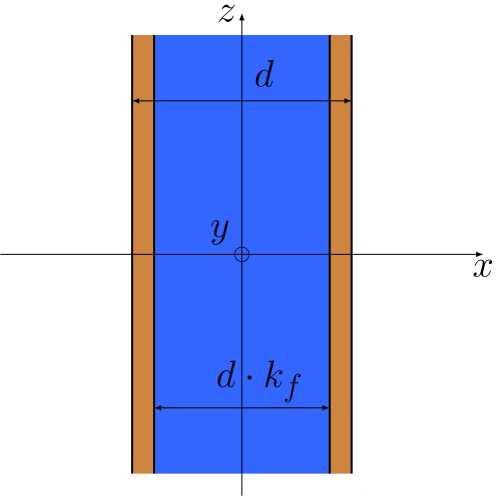
Figure 1: An infinite iron sheet (blue) with insulation (brown). The total thickness is $d$, and the thickness of the iron is $k_{f}d$, $k_{f}$ being the fill factor. The sheet is assumed to be infinite in the $y$ and $z$ directions.

II A Simplified Model and the Effective BH-Curve

We start with a simplified setup: a periodic structure whose lattice cell is an insulated iron sheet, infinite in the $y$- and $z$-directions (Fig. 1); the geometric parameters are indicated in the figure. A constant tangential component $h_{0}$ of the magnetic field $\mathbf{h}=h\hat{z}$ is prescribed at $x=\pm d/2$. The fine-scale magnetic field $\mathbf{h}$ satisfies Maxwell’s equations with the displacement current neglected. Under the harmonic balance approximation, well established in applied electromamgnetic analysis Yamada-harmonic-balance89 ; Paoli-Biro-complex-nonlinear98 ; Ausserhofer-Biro-harmonic-balance07 ; Biro-nonlinear-periodic14 , these equations are, in the SI system under the $\exp(+i\omega t)$ phasor convention, $\nabla\times\mathbf{e}=-i\omega\mathbf{b}$, $\nabla\times\mathbf{h}=\mathbf{j}$. The standard notation $\mathbf{e}$, $\mathbf{h}$, $\mathbf{b}$, $\mathbf{j}$ is used for the respective fields and eddy currents; small letters are reserved for fine-scale quantities; capital letters will be used later on to indicate coarse-scale (homogenized) fields. The material relations are considered to be intrinsically isotropic for simplicity: $\mathbf{b}\,=\,\mu(|\mathbf{h}|)\mathbf{h}$; $\mathbf{j}\,=\,\sigma\mathbf{e}$, $\sigma$ being the electric conductivity. For the setup of Fig. 1, the eddy current problem is one-dimensional:

$$-\partial_{x}\left(\rho\partial_{x}h(x)\right)\,+\,i\omega\mu(|h(x)|)\,h(x)\,=\,0;\quad\rho\equiv\sigma^{-1}$$ (1)

$$\mathbf{h}(x)=h(x)\hat{z};\quad h\left(-\frac{d}{2}\right)=h\left(\frac{d}{2}\right)=h_{0}$$

The active and reactive losses per unit length can be written as a single complex number:

$$P(h_{0})\,=\,\frac{1}{2}\int_{-d/2}^{d/2}\mathbf{e}\mathbf{j}^{*}\,dx~{}+~{}\frac{i\omega}{2}\int_{-d/2}^{d/2}\mathbf{h}\,\mathbf{b}^{*}\,dx.$$ (2)

By definition, the coarse-scale field cannot depend on $x$. Hence for the infinite sheet problem, the only possible effective field is a constant function $\mathbf{H}\equiv\mathbf{h}_{0}=h_{0}\hat{z}$. Because $\operatorname{curl}\mathbf{H}=0$, we define the effective losses as

$$P_{\mathrm{eff}}(h_{0})\,=\,\frac{i\omega\mu_{\mathrm{eff}}(h_{0})}{2}\int_{-d/2}^{d/2}|h_{0}|^{2}\,dx,$$ (3)

where $\mu_{\mathrm{eff}}(h_{0})$ is a complex number, to be determined by demanding $P(h_{0})=P_{\mathrm{eff}}(h_{0})$. Then, by varying $h_{0}$ and defining $\mathbf{B}=\mu_{\mathrm{eff}}(\mathbf{H})\mathbf{H}$, one obtains both real and imaginary parts of the effective BH-curve. Naturally, this curve depends on the frequency $\omega$, the electric conductivity $\sigma$, the thickness $d$ and the fill factor $k_{f}$ of the iron (Fig. 1).

Even though the effective complex BH-curve has been defined for this simplified setup, the numerical example in the following section shows that this curve gives quite accurate results for a realistic cylindrical geometry as well (Fig. 2).

III A Realistic Model with Cylindrical Geometry

We consider cylindrical geometry, typical for rotating machines. One lattice cell of a periodic stack (Fig. 2) is represented in the cylindrical coordinates $(r,z,\theta)$ as a rectangle whose width does not have to be small relative to the penetration depth $\delta=(2\rho/(\omega\mu))^{\frac{1}{2}}$. The domain of analysis is $\mathrm{\Omega}=[r_{\mathrm{min}},r_{\mathrm{max}}]\times[-d/2,d/2]$ in the $zr$ plane, The laminated structure occupies the region $[-d/2,d/2]\times[r_{\mathrm{in}},r_{\mathrm{out}}]$, of which $-w_{\mathrm{iron}}/2\leq z\leq w_{\mathrm{iron}}/2$ is the iron. Periodic boundary conditions link the magnetic fields at $z=\pm d/2$. On the exterior boundary outside the structure ($r=r_{\max}>r_{\mathrm{out}}$) the tangential component of the magnetic field is set to zero. The only conducting material in this model is iron.

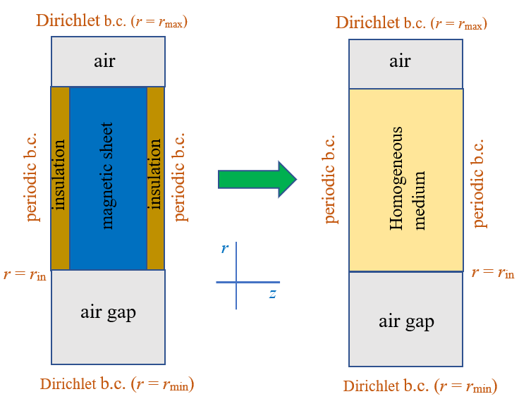
Figure 2: Setup: homogenization problem for laminated structures in cylindrical geometry.

Remark. The coarse-scale (homogeneous) field $\mathbf{H}$ cannot, by definition, depend on $z$ and, from symmetry considerations, must have a zero $z$ component. Hence $\mathbf{J}_{\phi}=(\nabla\times\mathbf{H})_{\phi}=0$. Due to insulation, the average $\langle j_{z}\rangle\equiv J_{z}=0$; then the remaining component $J_{r}$ is also zero, due to $\nabla\cdot\mathbf{J}=0$. Hence eddy currents cannot be represented on the coarse scale; this is why the physical nature of the problem changes upon homogenization.

For the fine-scale problem, we used the formulation in terms of the vector potential $\mathbf{t}=(t_{z},t_{r})$ of eddy currents and the magnetic scalar potential $u$. Then $\mathbf{h}=\mathbf{t}-\nabla u$; $\mathbf{t}$ vanishes outside the conducting regions, as does its tangential component on the boundary of these regions; also, $u=0$ at $r=r_{\max}$. (In general, a Dirichlet boundary condition $u=u_{D}$ is equivalent to $H_{\phi}=-u_{D}/r$.)

The $\mathbf{t}$-$u$ formulation (frequently also referred to as the $\mathbf{T}$-$\mathrm{\Omega}$ formulation) is very well known Carpenter77 ; Tsukerman90 ; Schoebinger19 ; Hollaus18 and has also been studied in the multiscale setting Hollaus19 . The mathematical equations and brief notes on their numerical solution are included as an Appendix.

On the coarse scale, the effective BH curve is complex-valued and derived by equating the fine- and coarse-scale losses (Section II). There are known instances where complex BH-curves were used in connection with the Preisach hysteresis modelHoBi:02 , but here they are used in the context of homogenization.

The homogenized (coarse-scale) problem is formulated as a magnetostatic one:

$$-\nabla\cdot\mu_{\mathrm{eff}}\nabla U\,=\,0$$ (4)

with $\mathbf{H}=\nabla U$ and the complex magnetic permeability $\mu_{\mathrm{eff}}$. The boundary conditions for $u$ and $U$ are identical.

IV Numerical Example

First we consider a cylindrical iron sheet, at a frequency of $f=500$ Hz, with the thickness $d=0.5$ mm, the fill factor $k_{f}=0.9$, and the electric conductivity $\sigma=2\cdot 10^{6}$ S/m. As in the previous section, the effective BH-curve was determined by equating the fine-scale and coarse-scale losses. Fig. 3 shows the actual and effective BH-curves corresponding to these parameters. The measurements were taken for a ring core which was incorporated within a computer-aided setup in acccordance with the international standard IEC 60404-6.

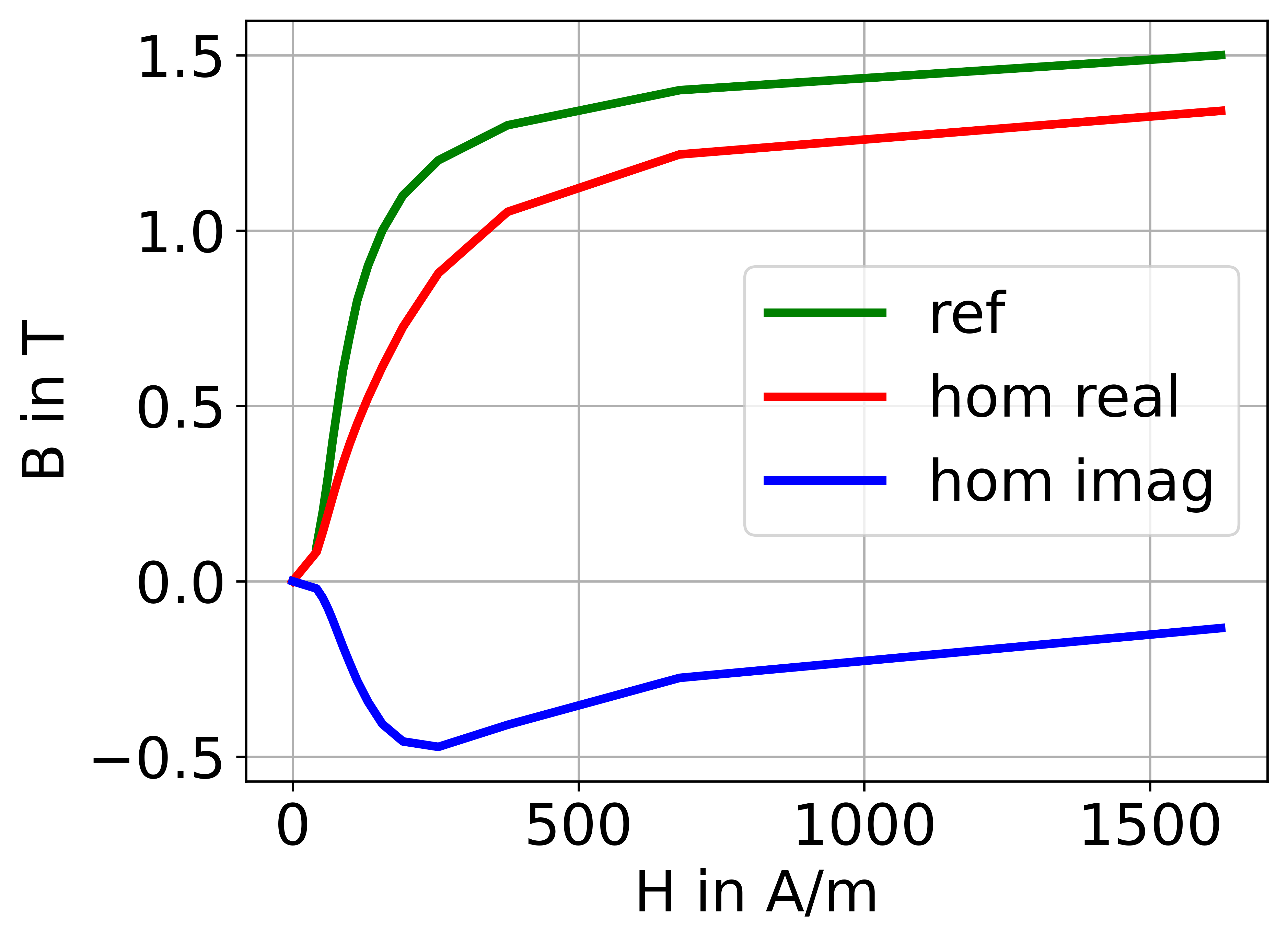
Figure 3: The BH-curve of the example material (green), as well as the real (red) and the imaginary (blue) part of the effective curve at $500$ Hz, obtained by the method described in section II.

Further, we choose as an example the geometry shown in Fig. 2. The iron sheet has the inner radius of $r_{\mathrm{in}}=24$ mm and the outer radius $r_{\mathrm{out}}=30$ mm. The inner and outer radii of the air gap are $r_{\min}=23$ mm and $r_{\max}=31$ mm, respectively.

Table 1 lists the active and reactive losses for different “excitation” conditions of $u_{D}$ at $r=r_{\min}$. For $u_{D}\,\lesssim\,50$ A, the material behaves almost linearly, while at $u_{D}=300$ A it is nearly fully saturated, as can be seen by the corresponding values for the $\mathbf{h}$ and $\mathbf{H}$, evaluated at the bottom of the sheet.

Table 1: Active Losses $P_{a}$ and Reactive Losses $P_{r}$ for Different Exitations at 500 Hz

$u_{D}$ in A	$|\mathbf{h}(r_{in})|$ in $A/m$	$|\mathbf{H}(r_{in})|$ in $A/m$	$P_{r}$, ref.  in mVA	$P_{r}$, hom. in mVA	$P_{a}$, ref. in mW	$P_{a}$, hom. in mW
$50$	73.6	74.8	$1.763$	$1.757$	$0.7197$	$0.7643$
$100$	115	118	$5.277$	$5.285$	$3.001$	$3.189$
$150$	170	175	$11.38$	$11.46$	$7.132$	$7.561$
$200$	255	264	$23.22$	$23.66$	$12.9$	$13.59$
$250$	443	460	$52.11$	$53.72$	$19.01$	$20.35$
$300$	894	909	$122.1$	$122.2$	$23.48$	$25.82$

Table 2 lists the errors of the homogenized solution with respect to the actual (fine-scale) one. The error in the potential is the difference $|U(r)-u(r)|$ at $r=r_{\mathrm{in}}$; this may also serve as a measure of the difference in the reaction fields.

Table 2: Relative Errors for Different Exitations at 500 Hz

$u_{D}$ in A	$\Delta P_{r}$ in $\%$	$\Delta P_{a}$ in $\%$	$\Delta u(r_{in})$ in $\%$
$50$	$0.33$	$6.2$	$2.0$
$100$	$0.15$	$6.3$	$2.7$
$150$	$0.73$	$6.0$	$2.8$
$200$	$1.9$	$5.3$	$2.7$
$250$	$3.1$	$7.0$	$3.6$
$300$	$0.11$	$10.0$	$1.7$

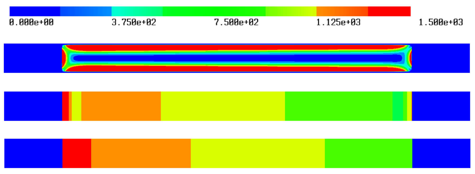
Figure 4: The eddy current losses in $W/\mathrm{m}^{3}$ for the reference solution (top), the reference solution averaged over the thickness (middle) and the homogeneous solution (bottom) for the excitation $u_{D}=100$ A at $500$ Hz.

It can be seen that all errors stay in the range of a few percent with a slight increase for higher saturation. Note that an error of zero would be impossible even for a fully linear material, because the effective material parameters were obtained from the infinite sheet and therefore cannot fully account for the edge effects, which are most prevalent at the shorter sides of the sheet.

Comparison of the distributions of the loss densities on the fine and coarse scales demonstrates that the homogenized problem accurately represents not only global but also local losses (Fig. 4). Fig. 5 shows the active and reactive components of the losses along the midline $x=0$, at low saturation of the iron. Fig. 6 shows similar distributions at a higher saturation. It can be seen that the homogeneous solution reproduces the distribution accurately, except for the edge effects, at low and high saturations.

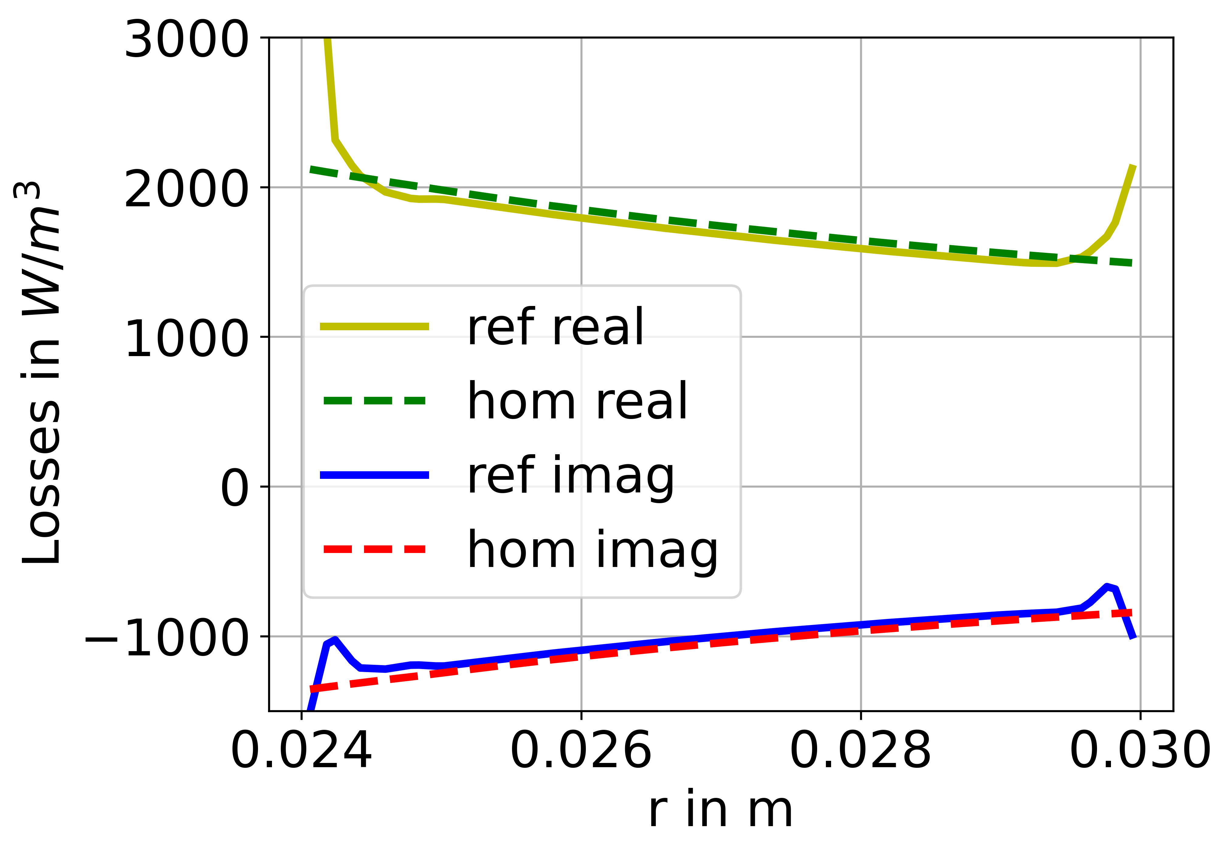
Figure 5: The complex losses for the fine-scale solution (solid lines, averaged over the thickness) and the homogeneous solution (dashed lines) along the midline $x=0$ for the excitation $u_{D}=100$ A at $500$ Hz.

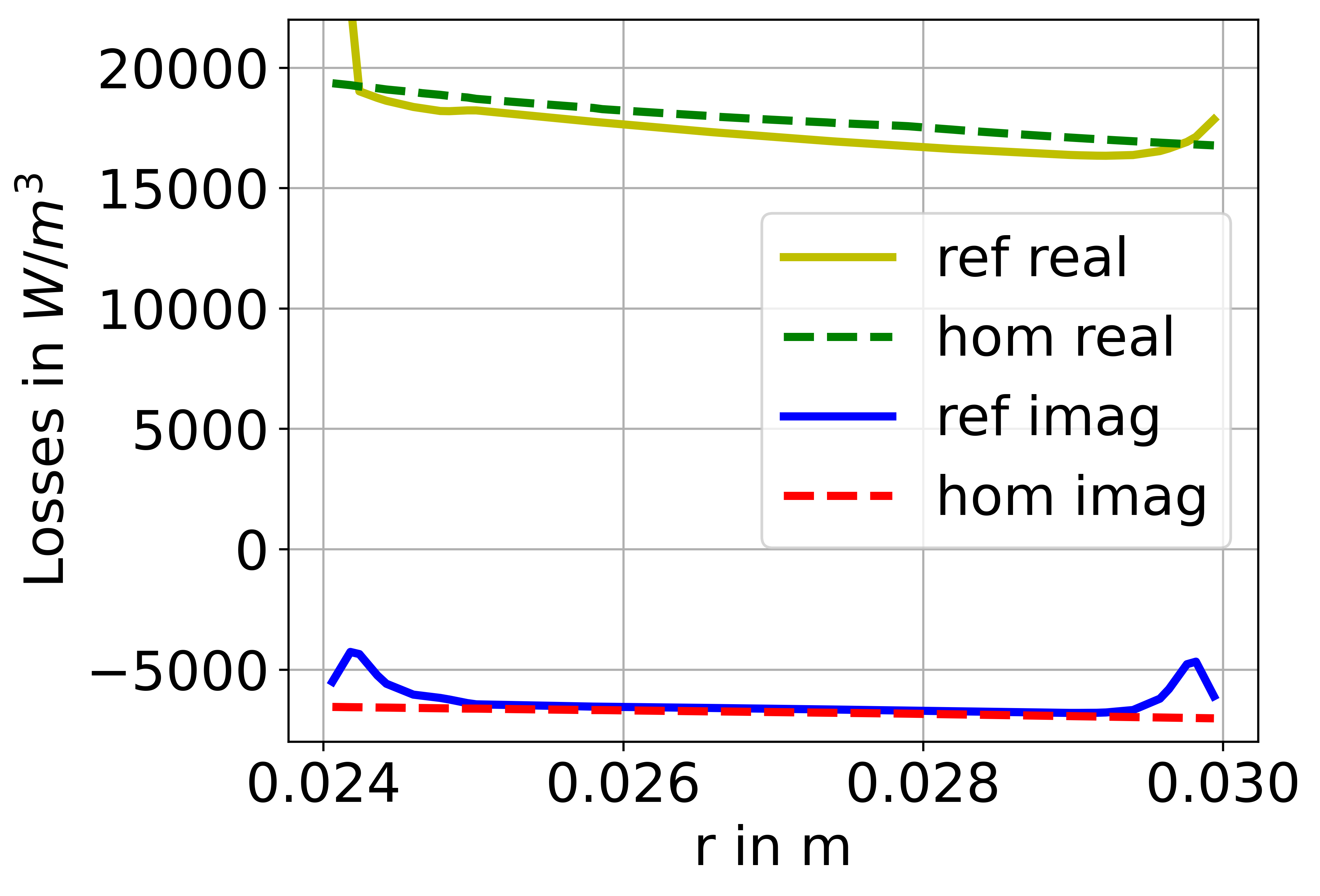
Figure 6: The complex losses for the fine-scale solution (solid lines, averaged over the thickness) and the homogeneous solution (dashed lines) along the midline $x=0$ for the excitation $u_{D}=250$ A at $500$ Hz.

For comparison, the BH-curve for the same material but at $f=50$ Hz are displayed in Fig. 7. As can be seen in Table 3, the results are lower overall than at $f=500$ Hz.

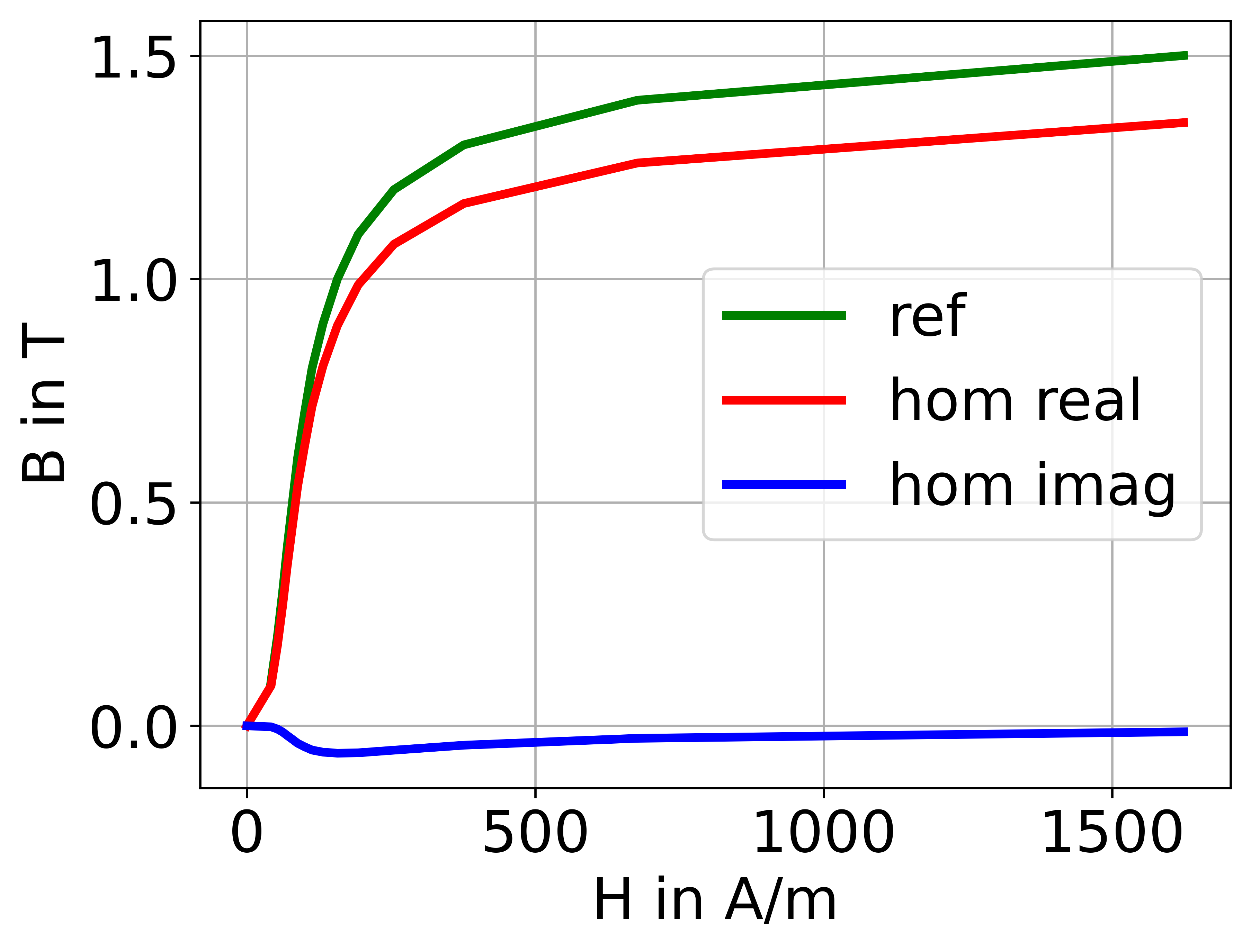
Figure 7: The BH-curve of the example material (green), as well as the real (red) and the imaginary (blue) parts of the effective curve at $f=50$ Hz.

Table 3: Relative Errors for Different Exitations at 50 Hz

$u_{D}$ in A	$\Delta P_{r}$ in $\%$	$\Delta P_{a}$ in $\%$	$\Delta u(r_{in})$ in $\%$
$50$	$0.07$	$4.8$	$0.3$
$100$	$0.4$	$5.6$	$0.34$
$150$	$0.16$	$4.9$	$0.32$
$200$	$0.6$	$5.3$	$0.61$
$250$	$1.2$	$7.3$	$0.97$
$300$	$3.0$	$11.2$	$2.4$

V Conclusion

The fine-scale eddy current problem examined in this Letter changes its physical nature upon homogenization, when a stratified nonlinear magnetic medium is replaced with an effective homogeneous one. Namely, the appropriate coarse-scale (homogeneous) model is, counter-intuitively, magnetostatic, with a nonlinear complex-valued BH-curve whose real and imaginary parts represent active and reactive losses in the iron. In addition, the reaction field of the structure is also represented accurately on the coarse scale. These results may be relevant in other physical and engineering applications, where similar problems – especially diffusion problems with boundary layers – may arise.

Appendix: The Mathematical Formulation

The key equations for the eddy current problem under consideration are, in weak form,

$$(\mu\nabla u,\nabla u^{\prime})-(\mu\mathbf{t},\nabla u^{\prime})\,=\,-(\mu\nabla u_{D},\nabla u^{\prime})$$ (5)

$$(\sigma^{-1}\nabla\times\mathbf{t},\nabla\times\mathbf{t}^{\prime})-i\omega(\mu\mathbf{t},\mathbf{t}^{\prime})+i\omega(\mu\nabla u,\mathbf{t}^{\prime})\,=\,0.$$ (6)

In these equations, parentheses denote the $L_{2}^{3}$ inner products of vector functions; $u,u^{\prime}\in H_{0}^{1}(\mathrm{\Omega})$, $\mathbf{t},\mathbf{t}^{\prime}\in H_{0}(\mathrm{curl},\mathrm{\Omega}_{\mathrm{iron}})$; the primed symbols denote arbitrary test functions in their respective spaces. Definitions of the function spaces and their discretizations using high-order edge elements for $\mathbf{t}$ and nodal elements for $u$ can be found in SchoeZagl:05 . All simulations were done using the open-source package Netgen/NGSolve NGSolve .

References

- [1] D. J. Bergman. Dielectric-constant of a composite-material – problem in classical physics. Physics reports – Review section of Physics Letters, 43(9):378–407, 1978.
- [2] A. Bensoussan, J.L. Lions, and G. Papanicolaou. Asymptotic Methods in Periodic Media. North Holland, 1978.
- [3] N. S. Bakhvalov and G. Panasenko. Homogenisation: Averaging Processes in Periodic Media, Mathematical Problems in the Mechanics of Composite Materials. Springer, 1989.
- [4] Graeme Milton. The Theory of Composites. Cambridge University Press: Cambridge ; New York, 2002.
- [5] David R. Smith and John B. Pendry. Homogenization of metamaterials by field averaging. J. of the Optical Soc. of America B, 23(3):391–403, 2006.
- [6] G. Bouchitté and B. Schweizer. Homogenization of Maxwell’s equations in a split ring geometry. Multiscale Modeling & Simulation, 8(3):717–750, 2010.
- [7] Vadim A. Markel and John C. Schotland. Homogenization of maxwell’s equations in periodic composites: Boundary effects and dispersion relations. Phys. Rev. E, 85:066603, Jun 2012.
- [8] Igor Tsukerman and Vadim A. Markel. A nonasymptotic homogenization theory for periodic electromagnetic structures. Proc Royal Soc A, 470:2014.0245, 2014.
- [9] Igor Tsukerman. Classical and non-classical effective medium theories: New perspectives. Physics Letters A, 381(19):1635–1640, 2017.
- [10] C. W. Nan, Y. Shen, and Jing Ma. Physical properties of composites near percolation. In Clarke, DR and Ruhle, M and Zok, F, editor, Annual Review of Materials Research, volume 40 of Annual Review of Materials Research, pages 131–151. 2010.
- [11] Pochi Yeh. Optical Waves in Layered Media. Hoboken, N.J.: John Wiley, 2005.
- [12] Igor Tsukerman, A N M Shahriyar Hossain, and Y. D. Chong. Homogenization of layered media: Intrinsic and extrinsic symmetry breaking. arXiv:2003.08492; submitted, 2020.
- [13] J. Gyselinck, R. V. Sabariego, and P. Dular. A nonlinear time-domain homogenization technique for laminated iron cores in three-dimensional finite-element models. IEEE Trans Magn, 42(4):763–766, 2006.
- [14] O. Bottauscio and M. Chiampi. Analysis of laminated cores through a directly coupled 2-D/1-D electromagnetic field formulation. IEEE Trans Magn, 38(5):2358–2360, 2002.
- [15] I. Niyonzima, R. V. Sabariego, P. Dular, F. Henrotte, and C. Geuzaine. Computational homogenization for laminated ferromagnetic cores in magnetodynamics. IEEE Trans Magn, 49(5):2049–2052, 2013.
- [16] I. Niyonzima, C. Geuzaine, and S. Schöps. Waveform relaxation for the computational homogenization of multiscale magnetoquasistatic problems. J Comp Phys, 327:416–433, 2016.
- [17] K. Hollaus and J. Schöberl. A higher order multi-scale FEM with for 2-D eddy current problems in laminated iron. IEEE Trans Magn, 51(3):1–4, 2015.
- [18] K. Hollaus and J. Schöberl. Some 2-d multiscale finite-element formulations for the eddy current problem in iron laminates. IEEE Trans Magn, 54(4):1–16, 2018.
- [19] S Yamada, K Bessho, and J Lu. Harmonic-balance finite-element method applied to nonlinear AC magnetic analysis. IEEE Trans Magn, 25(4):2971–2973, 1989.
- [20] G Paoli, O Biro, and C Buchgraber. Complex representation in nonlinear time harmonic eddy current problems. IEEE Trans Magn, 34(5, 1):2625–2628, 1998.
- [21] Stefan Ausserhofer, Oszkar Biro, and Kurt Preis. An efficient harmonic balance method for nonlinear eddy-current problems. IEEE Trans Magn, 43(4, SI):1229–1232, 2007.
- [22] Oszkar Biro, Gergely Koczka, and Kurt Preis. Finite element solution of nonlinear eddy current problems with periodic excitation and its industrial applications. Appl Num Math, 79(SI):3–17, 2014.
- [23] C. J. Carpenter. Comparison of alternative formulations of 3-dimensional magnetic-field and eddy-current problems at power frequencies. Proceedings of the Institution of Electrical Engineers, 124(11):1026–1034, 1977.
- [24] I.A. Tsukerman. Error estimation for finite-element solutions of the eddy currents problem. COMPEL, 9(2):83–98, 1990.
- [25] M. Schöbinger, J. Schöberl, and K. Hollaus. Multiscale FEM for the linear 2-D/1-D problem of eddy currents in thin iron sheets. IEEE Trans Magn, 55(1):1–12, 2019.
- [26] K. Hollaus and M. Schöbinger. A multiscale FEM for the eddy current problem with in laminated conducting media. IEEE Trans Magn, 56(4):1–4, April 2020.
- [27] Karl Hollaus and Oszkár Bíró. Derivation of a complex permeability from the Preisach model. IEEE Trans. Magn., 38(2):905–908, 2002.
- [28] Joachim Schöberl and Sabine Zaglmayr. High order Nédélec elements with local complete sequence properties. COMPEL, 24(2):374–384, 2005.
- [29] Joachim Schöberl. Netgen/NGSolve, https://ngsolve.org/.
- [30] R Albanese, E Coccorese, R Martone, G Miano, and G Rubinacci. Periodic-solutions of nonlinear eddy-current problems in 3-dimensional geometries. IEEE Trans Magn, 28(2):1118–1121, 1992.
- [31] Oszkar Biro, Gergely Koczka, and Kurt Preis. Finite element solution of nonlinear eddy current problems with periodic excitation and its industrial applications. Appl Num Math, 79(SI):3–17, 2014.
- [32] W. E, B. Engquist, X. Li, W. Ren, and E. Vanden-Eijnden. Heterogeneous multiscale methods: A review. Comm Comp Phys, 2(3):367–450, 2007.
- [33] J. Gyselinck and P. Dular. A time-domain homogenization technique for laminated iron cores in 3-d finite-element models. IEEE Trans Magn, 40(2):856–859, 2004.
- [34] J. Gyselinck, R. V. Sabariego, and P. Dular. A nonlinear time-domain homogenization technique for laminated iron cores in three-dimensional finite-element models. IEEE Trans Magn, 42(4):763–766, 2006.
- [35] J. Gyselinck, P. Dular, L. Krähenbühl, and R. V. Sabariego. Finite-element homogenization of laminated iron cores with inclusion of net circulating currents due to imperfect insulation. IEEE Trans Magn, 52(3):1–4, 2016.
- [36] K. Hollaus, A. Hannukainen, and J. Schöberl. Two-scale homogenization of the nonlinear eddy current problem with FEM. IEEE Trans Magn, 50(2):413–416, 2014.
- [37] Paul Penfield and H. A. Haus. Electrodynamics of Moving Media. The MIT Press, 1967.
- [38] M. Schöbinger, K. Hollaus, and I. Tsukerman. Nonasymptotic homogenization of laminated magnetic cores. IEEE Trans Magn, 56:7509504, February 2020.
- [39] Sabine Zaglmayr. High Order Finite Element Methods for Electromagnetic Field Computation. PhD thesis, Johannes Kepler Universität,Linz,Austria, 2006.
- [40] J. Gyselinck and P. Dular. A time-domain homogenization technique for laminated iron cores in 3-D finite-element models. IEEE Trans. Magn., 40(2):856–859, 2004.