Galaxy redshift-space bispectrum: the Importance of Being Anisotropic

D. Gualdi    L. Verde
Abstract

We forecast the benefits induced by adding the bispectrum anisotropic signal to the standard, two- and three-point, clustering statistics analysis. In particular, we forecast cosmological parameter constraints including the bispectrum higher multipoles terms together with the galaxy power spectrum (monopole plus quadrupole) and isotropic bispectrum (monopole) data vectors. To do so, an analytical covariance matrix model is presented. This template is carefully calibrated on well-known terms of a numerical covariance matrix estimated from a set of simulated galaxy catalogues. After testing the calibration using the power spectrum and isotropic bispectrum measurements from the same set of simulations, we extend the covariance modelling to the galaxy bispectrum higher multipoles. Using this covariance matrix we proceed to perform cosmological parameter inference using a suitably generated mock data vector. Including the bispectrum mutipoles up to the hexadecapole, yields 1-D 68%percent6868\% credible regions for the set of parameters (b1,b2,f,σ8,fNL,α,α)subscript𝑏1subscript𝑏2𝑓subscript𝜎8subscript𝑓NLsubscript𝛼perpendicular-tosubscript𝛼parallel-to(b_{1},b_{2},f,\sigma_{8},f_{\mathrm{NL}},\alpha_{\perp},\alpha_{\parallel}) tighter by a factor of 30%percent\% on average for kmax=0.09hsubscript𝑘max0.09k_{\mathrm{max}}=0.09\,h/Mpc, significantly reducing at the same time the degeneracies present in the posterior distribution.

1 Introduction

Higher-order statistics represent the most direct tool to access the cosmological information encrypted in the non-Gaussian features of the matter density field. Three-point (3pt) statistics are the lowest order, and therefore the simplest, tools enabling us to harvest this information. The most recent analyses for the Baryon Oscillation Spectroscopic Survey (BOSS) [3] spectroscopic data-set, part of the Sloan Digital Sky Survey (SDSS) [34], have been performed for both the 3pt correlation function [87] and its Fourier transform, the bispectrum [44].

Approximately four decades have passed since the first 3pt statistics studies [45, 70, 39, 36]. However only twenty years ago a mature formalism was developed to map theoretical models to spectroscopic data-sets in redshift space [66, 92, 94, 78, 77, 79, 81].

The window on non-linear scales was opened with the loop corrections inclusion [83, 86, 52, 31, 33, 24]; higher-order terms become important at non-linear scales and are indeed necessary to study primordial non-Gaussianity using the 3pt statistics to lift the degeneracy with the other cosmological parameters [93, 82, 57, 18, 60].

The general benefits of using the bispectrum in addition to the power spectrum have recently been studied in [96, 69, 9]. Originally, the bispectrum was thought to be useful in order to break the degenaracies between bias and cosmological parameters [38, 37]. Lately, the bispectrum has been shown to be a key tool for reaching more specific goals, such as detecting General Relativity effects [42, 11, 12, 14, 32] and improving the neutrino masses constraints [75, 29, 49].

Nevertheless, all the analyses performed to date on spectroscopic data have been limited to the isotropic signal component, the so-called bispectrum "monopole" [43, 44]. In analogy to the power spectrum, redshift space distortions (RSD) induce an anisotropic signal with respect to the line of sight (see pioneering work by [59, 50]). This anisotropy can be expanded in multipole moments, where the monopole is just the averaged signal in all directions around the line of sight. To date, multipoles beyond the monopole have been used to constrain cosmological parameters only for the power spectrum [67, 68, 15, 17], with the state-of-the-art at the moment of writing being Refs. [16, 97, 55, 54, 72, 28]. Measuring higher-order multipoles of the redshift-space galaxy bispectrum is complicated in terms of estimators modelling [76, 52, 89], even when simulated volumes with periodic boundary conditions are used. For galaxy surveys, these measurements are even more difficult because of the necessity of accounting for all observational effects (e.g., window function effect, varying average density number, varying line of sight, etc.). As in the case of the power spectrum, the anisotropic signal in the bispectrum due to RSD potentially carries key additional cosmological information.

This additional signal can be used not only to obtain tighter parameter constraints, but also as a self-consistency check for the theoretical model itself. In other words one could test whether the same set of cosmological parameters can produce an analytical template that fits well all the measured data vector components (power spectrum / bispectrum, isotropic / anisotropic). Hence we have a strong motivation to investigate the potential of the galaxy bispectrum multipoles.

The purpose of this work is to assess the added constraining power obtained by including higher-order multipoles of the bispectrum to the so far used large scale structure (LSS) statistics in Fourier space (power specrum multipoles and bispectrum monopole). We study the improvements, in terms of tighter parameter constraints, in the 1- and 2-D 68%percent6868\% credible regions resulting from using the bispectrum multipoles. Fisher forecasts for the bispectrum multipoles, using a diagonal covariance matrix including only Gaussian terms, were realised in [40]. Here we go beyond this approximation, dedicating a significant effort in modelling the off-diagonal, non-Gaussian terms of the covariance matrix.

Since measurements of these new statistics (the anisotropic bispectrum modulation) either from mocks or data are at the moment extremely expensive and the necessary codes are not fully developed or publicly available yet, it is important to estimate first the potential gain these new statistics could offer. To do so however the full covariance matrix must be estimated in order to derive the cosmological parameters posterior distributions, for example through Markov Chain Monte Carlo methods (MCMC). We argue here that resorting to MCMC’s is indeed necessary to explore and place constraints on parameters-space where there are non-trivial degeneracies, such as the parameters usually constrained in a clustering analysis. Fisher forecast can not do this since are based on the first derivatives of the data-vector’s theoretical model.

Note that the covariance must be estimated for the full "data vector" which comprises both the power spectrum and bispectrum multipoles; this matrix cannot be approximated as diagonal. Traditionally, there are two approaches to estimate covariance matrices: from a large number of mocks or analytically. Adopting the first approach alone is not viable here, for the reason explained above that measurements of these statistics from a large enough set of mocks are not currently available. Therefore we model the covariance matrix analytically, calibrating it, as much as possible, for the terms that are measurable, on estimates from a large number of mocks. We then use this analytical template, calibrated and extended to terms involving the bispectrum higher multipoles, to evaluate the likelihood in the MCMC sampling of the parameters posterior distribution.

An analytical model of the galaxy power spectrum and bispectrum multipoles covariance matrix alternative to the one presented here, was recently derived in [88], where the effect of including the anisotropic bispectrum signal was studied through the cumulative signal to noise ratio.

In order to model the galaxy bispectrum higher multipoles we use the choice of angles described in [52] which differs from the one recently proposed in [89]. The expansion is then performed in terms of the angle between the normal to the triangle’s surface and the line of sight, together with the angle describing the rotation of the triangle on the plane defined by its sides (or in other words the rotation around the normal to the triangle’s surface).

The structure of the paper is the following. In Section 2 we give an overview of the objectives and the necessary steps to achieve them. In Section 3 we describe the analytical expressions used to model the data vector while in Section 4 we list the analytical terms that we included in our covariance matrix model. Section 5 is of critical importance since it describes the qualitative and quantitative tests that we performed in order to check the accuracy and reliability of our covariance analytical model. In Section 6 we forecast through MCMC sampling the parameter constraints improvements obtained by adding to the data vector the galaxy bispectrum higher multipoles. We conclude in Section 7.
Refer to caption
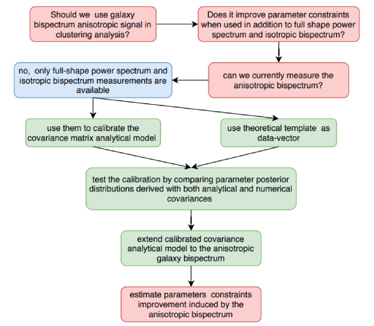
Figure 1: Conceptual map of the paper.

2 Statement of the problem, objectives and roadmap

It is not at all a trivial task to develop the estimators and the associated numerical pipelines to measure the galaxy-redshift space bispectrum anisotropic signal in terms of multipoles expansion [76, 88]. Hence it is important to ask: is it worth it? There are two aspects to this question. One is the simple potential in reducing parameters errors or lifting parameters degeneracies. The other aspect is that in any practical application, these extra statistics can offer a powerful consistency check of the modelling and thus possibly of the model itself. The second aspect, while possibly of more consequence than the first, cannot be easily demonstrated and quantified before one is able to measure these statistics on mock survey catalogs (mocks for short). However, it is reasonable to expect that these statistics can provide a useful consistency checks if they carry significant additional information, and therefore only if they are useful to reduce parameters errors. This is what we set up to address in this work.

Our goal is indeed to show whether adding the bispectrum anisotropic signal to the standard power spectrum Pg()superscriptsubscriptPg\mathrm{P}_{\mathrm{g}}^{(\ell)} (isotropic + anisotropic) and bispectrum Bg(00)superscriptsubscriptBg00\mathrm{B}_{\mathrm{g}}^{(00)} (isotropic) data vector, produces tighter 1-2D marginalised posterior distributions for the parameters usually constrained by galaxy-clustering analyses. We prove this through the path described in the conceptual map of Figure  1.

Given the absence of measurements, the first task consists in analytically modelling the bispectrum anistropic signal. We choose a decomposition in terms of Legendre polynomials for a specific choice of angles describing the orientation with respect to the line of sight. We then proceed to use this theoretical model as a "mock"111The meaning of ”mock” here is different from the more widespread use of the term. Usually ”mock” data refer to carefully simulated data in such a way as to have properties as similar as possible to the real data. Here our generated data vector is somewhat idealized, being obtained from theoretical templates. For this reason we use the term ”mock” here in quotes. In the rest of the paper we will use the word mock in its more common meaning and refer for brevity to the template-generated data as (fiducial) template data vector. In some applications we will use a data vector obtained from the survey mocks. We will refer to this as simulated data vector. data vector. A similar approach was used in [71, 19] to derive forecasts on the sum of the neutrino masses constraints.

In summary our "data" vector is composed by four blocks, galaxy power spectrum (isotropic plus anisotropic) and galaxy bispectrum (also isotropic plus anisotropic):
[Pg(0);Pg(2);Bg(00);Bg(ıȷ)]subscriptsuperscriptP0gsubscriptsuperscriptP2gsubscriptsuperscriptB00gsubscriptsuperscriptBitalic-ıitalic-ȷg\left[\mathrm{P}^{(0)}_{\mathrm{g}};\mathrm{P}^{(2)}_{\mathrm{g}};\mathrm{B}^{(00)}_{\mathrm{g}};\mathrm{B}^{(\imath\jmath)}_{\mathrm{g}}\right], where Bg(ıȷ)subscriptsuperscriptBitalic-ıitalic-ȷg\mathrm{B}^{(\imath\jmath)}_{\mathrm{g}} indicates all the possible bispectrum higher multipoles. Each power spectrum block includes all the k𝑘k-bins (bandpowers) while each bispectrum block contains all the triangle configurations used.

As it is widely done in large-scale structure studies, we assume the likelihood of our data vector to be Gaussian, with a covariance matrix that does not depend on the cosmological parameters. This assumption has been extensively discussed, tested, and motivated, see e.g., [23, 73] for an insightful discussion.

To perform likelihood-based parameter inference, we also need the covariance matrix. The covariance matrix is usually estimated numerically from the data vector’s measurements on a large enough set of simulations or mock survey data. In our case we only have measurements for a reduced data vector which includes the standard galaxy clustering statistics, [Pg();Bg(00)]superscriptsubscriptPgsuperscriptsubscriptBg00\left[\mathrm{P}_{\mathrm{g}}^{(\ell)};\mathrm{B}_{\mathrm{g}}^{(00)}\right] and therefore only for a sub-matrix. To overcome this obstacle, we derive an analytical model for the full covariance matrix to be used as a template. This template can then be calibrated using the numerically estimated covariance for the sub matrix involving [Pg();Bg(00)]superscriptsubscriptPgsuperscriptsubscriptBg00\left[\mathrm{P}_{\mathrm{g}}^{(\ell)};\mathrm{B}_{\mathrm{g}}^{(00)}\right], for which we have measurements from 1400 galaxy mock catalogues. The calibration is done by fitting parameters which are common to both the anisotropic and isotropic components of the full data vector’s covariance and therefore independent of the multipole expansion. Two of them are amplitudes parameters (one for each of the power spectrum and bispectrum parts respectively) and the third one is an effective average galaxy number density (modelling the shot-noise). The fit is done by comparing our analytical template to the covariance matrix diagonal estimated from the mocks. For the calibration we only use the diagonal elements since they are signal-dominated (i.e., their statistical noise is negligible with respect to the physical signal). A similar approach was followed by Ref.  [87] to compute the three-point correlation function’s covariance matrix . In the analytic expression for the covariance matrix it is hard to include the extra mode-coupling and coupling between different statistics, induced by the window. This will be taken into consideration when performing the comparison to the numerical estimate of the covariance.

We use the analytical model for the power spectrum multipoles covariance only for the calibration process. In our forecasts, in order to minimize potential systematic errors connected with the power spectrum covariance modelling, for this part of the data vector, [Pg()]delimited-[]superscriptsubscriptPg\left[\mathrm{P}_{\mathrm{g}}^{(\ell)}\right], we will use the covariance numerically estimated from the simulations. The resulting "hybrid" covariance model will be referenced as HYB in the figures.

The following step is to verify that our covariance analytical model, when used to sample via a Markov chain Monte Carlo (MCMC) the parameters posterior distribution, produces the same results obtained with the numerical covariance matrix.

We test this for the case of the anisotropic power spectrum plus isotropic bispectrum data vector (for which we have measurements from a large set of galaxy mock catalogues). In particular we compare the posterior distributions 1D medians and 68%percent6868\% credible intervals for a set of 1400 galaxy mock catalogues.

Provided that there is no significant difference between the parameters posteriors obtained using the analytical covariance matrix template and the numerically estimated one, we can assume that the calibrated covariance model can safely be extended to the bispectrum multipoles.

The analytical model of the extended covariance matrix can then be used to evaluate the effect on cosmological parameter inference of including higher bispectrum multipoles in the data vector.

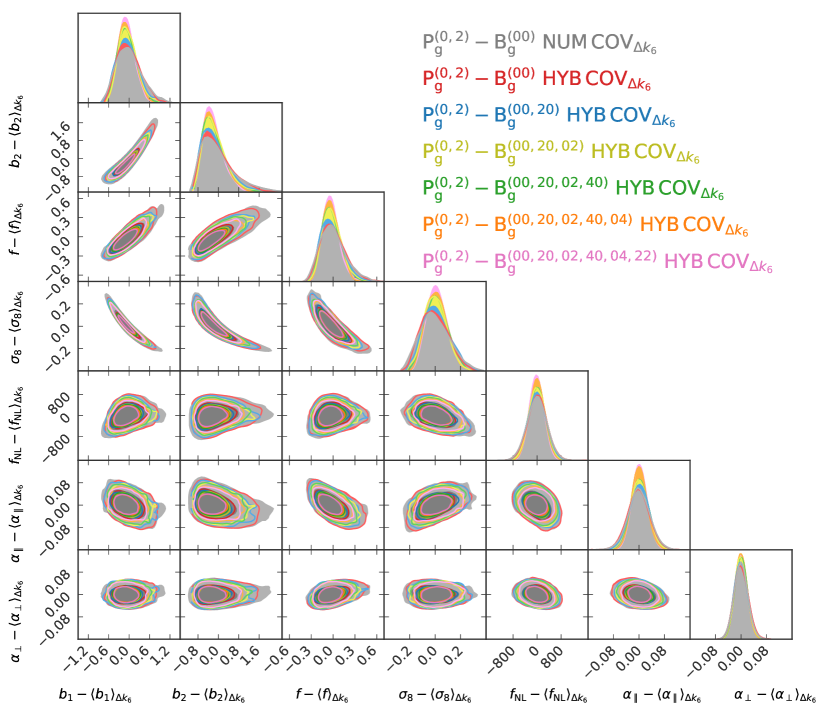
We will show in Section 6.2 two main results. First we prove that the anisotropic bispectrum signal contains additional significant cosmological information. Second, this improvement saturates at the level of the hexadecapole terms, meaning that measuring higher multipoles is not expected to further tighten parameter constraints (i.e., it would not be worth the effort).

3 Signal modelling

Given the lack of measurements from simulations or "real world" surveys, in our work we simulate the bispectrum anisotropic signal using an analytical template. Therefore we employ theoretical expressions derived from standard perturbation theory (see [13] for a complete review) to generate our "fiducial" (but realistic) template data vector.

The tree-level expression for the power spectrum and bispectrum are:

Pg(𝐤)subscriptPg𝐤\displaystyle\mathrm{P}_{\mathrm{g}}\left(\mathbf{k}\right) =Z1s[𝐤]2Pm(k)DFoGP(k)absentsubscriptsuperscriptZs1superscriptdelimited-[]𝐤2subscriptPm𝑘superscriptsubscript𝐷𝐹𝑜𝐺𝑃𝑘\displaystyle=\mathrm{Z^{\mathrm{s}}_{1}}\left[\mathbf{k}\right]^{2}\mathrm{P}_{\mathrm{m}}\left(k\right)D_{FoG}^{P}(k)
Bg(𝐤1,𝐤2,𝐤3)subscriptBgsubscript𝐤1subscript𝐤2subscript𝐤3\displaystyle\mathrm{B}_{\mathrm{g}}\left(\mathbf{k}_{1},\mathbf{k}_{2},\mathbf{k}_{3}\right)\, =[2Pm(k1)Pm(k2)Z1s[𝐤1]Z1s[𝐤2]Z2s[𝐤1,𝐤2]\displaystyle=\,\left[2\,\mathrm{P}_{\mathrm{m}}\left(k_{1}\right)\mathrm{P}_{\mathrm{m}}\left(k_{2}\right)\mathrm{Z^{\mathrm{s}}_{1}}\left[\mathbf{k}_{1}\right]\mathrm{Z^{\mathrm{s}}_{1}}\left[\mathbf{k}_{2}\right]\mathrm{Z^{\mathrm{s}}_{2}}\left[\mathbf{k}_{1},\mathbf{k}_{2}\right]\right.
+twocyclicterms]×DFoGB(k1,k2,k3),\displaystyle+\,\left.\mathrm{two\,cyclic\,terms}\right]\times D_{FoG}^{B}(k_{1},k_{2},k_{3}), (3.1)

where the subscript "g" indicates that the statistics are computed for the galaxy field in redshift space. The standard perturbation theory kernels in redshift space used in this work (ZnssubscriptsuperscriptZs𝑛\mathrm{Z}^{\mathrm{s}}_{n}) are those reported in Appendix C of [43]. The DFoGsubscript𝐷𝐹𝑜𝐺D_{FoG} terms model the Fingers-of-God effect (hereafter FoG) [56] introducing two effective parameters σPsubscript𝜎P\sigma_{\mathrm{P}} and σBsubscript𝜎B\sigma_{\mathrm{B}} for the power spectrum and bispectrum respectively. These parameters enter into two Lorentzian damping functions in front of the respective data vectors [43]:

DFoGPsuperscriptsubscript𝐷𝐹𝑜𝐺𝑃\displaystyle D_{FoG}^{P} =11+k2μ2σP2/2absent11superscript𝑘2superscript𝜇2superscriptsubscript𝜎P22\displaystyle=\dfrac{1}{1+k^{2}\mu^{2}\sigma_{\mathrm{P}}^{2}/2}\,
DFoGBsuperscriptsubscript𝐷𝐹𝑜𝐺𝐵\displaystyle D_{FoG}^{B} =11+(k12μ12+k22μ22+k32μ32)σB2/2.absent11superscriptsubscript𝑘12superscriptsubscript𝜇12superscriptsubscript𝑘22superscriptsubscript𝜇22superscriptsubscript𝑘32superscriptsubscript𝜇32superscriptsubscript𝜎B22\displaystyle=\,\dfrac{1}{1+(k_{1}^{2}\mu_{1}^{2}+k_{2}^{2}\mu_{2}^{2}+k_{3}^{2}\mu_{3}^{2})\sigma_{\mathrm{B}}^{2}/2}\,. (3.2)

Beside depending on the k𝑘k-vectors coordinates, the ZnssuperscriptsubscriptZns\mathrm{Z_{n}^{s}} kernels are also a function of the bias parameters b1subscript𝑏1b_{1}, b2subscript𝑏2b_{2} and bs2subscript𝑏superscript𝑠2b_{s^{2}} together with the growth rate f𝑓f.

As is it widespread, we also make the approximation of the bias being local in Lagrangian space, which allows us to express the non-local bias term bs2subscript𝑏superscript𝑠2b_{s^{2}} as function of the linear bias parameter b1subscript𝑏1b_{1}, bs2=47(b11)subscript𝑏superscript𝑠247subscript𝑏11b_{s^{2}}=-\dfrac{4}{7}(b_{1}-1) [26, 7, 43].

In our modeling and analysis we include the Alcock-Paczyǹski [5] parameters to account for differences between the true underlying cosmology and the fiducial one used to convert redshift measurements into Euclidean distances. A discrepancy between the fiducial and true underlying cosmology induces distortions in the clustering properties. This can be modelled through the parallel and perpendicular dilation parameters α=k/psubscript𝛼parallel-tosubscript𝑘parallel-tosubscript𝑝parallel-to\alpha_{\parallel}=k_{\parallel}/p_{\parallel} and α=k/psubscript𝛼perpendicular-tosubscript𝑘perpendicular-tosubscript𝑝perpendicular-to\alpha_{\perp}=k_{\perp}/p_{\perp} which relate the measured wave-vector 𝐤𝐤\mathbf{k} with the corresponding wave-vector 𝐩𝐩\mathbf{p} for a particular cosmology. Being μ𝜇\mu and η𝜂\eta the cosines of the angles between the line of sight and 𝐤𝐤\mathbf{k} and 𝐩𝐩\mathbf{p} respectively, the conversion is given by [44]

p𝑝\displaystyle p =|𝐩|=kα[1+μ2(F21)]12absent𝐩𝑘subscript𝛼perpendicular-tosuperscriptdelimited-[]1superscript𝜇2superscript𝐹2112\displaystyle=|\mathbf{p}|=\dfrac{k}{\alpha_{\perp}}\left[1+\mu^{2}\left(F^{-2}-1\right)\right]^{\frac{1}{2}}
η𝜂\displaystyle\eta =μF[1+μ2(F21)]12,absent𝜇𝐹superscriptdelimited-[]1superscript𝜇2superscript𝐹2112\displaystyle=\dfrac{\mu}{F}\left[1+\mu^{2}\left(F^{-2}-1\right)\right]^{-\frac{1}{2}}\,, (3.3)

where Fα/α𝐹subscript𝛼parallel-tosubscript𝛼perpendicular-toF\equiv\alpha_{\parallel}/\alpha_{\perp}.

3.1 Multipole expansion

We compute the multipole expansion of the tree-level galaxy power spectrum with respect to the line of sight in the standard way

Pg()(k)=(2+1)2αα21+1𝑑μ(μ)Pg(p,η)superscriptsubscriptPg𝑘212subscript𝛼parallel-tosuperscriptsubscript𝛼perpendicular-to2subscriptsuperscript11differential-d𝜇subscript𝜇subscriptPg𝑝𝜂\displaystyle\mathrm{P}_{\mathrm{g}}^{(\ell)}(k)=\dfrac{(2\ell+1)}{2\alpha_{\parallel}\alpha_{\perp}^{2}}\int^{+1}_{-1}d\mu\,\mathcal{L}_{\ell}(\mu)\,\mathrm{P}_{\mathrm{g}}(p,\eta)\, (3.4)

where μ𝜇\mu is the cosine of the angle between the line of sight and the k𝑘k-vector while (μ)subscript𝜇\mathcal{L}_{\ell}(\mu) is the \ell-th order Legendre polynomial.

For the bispectrum multipole expansion we adopt the choice of angles presented in [52]. The first angle is the one between the normal to the surface of the triangle and the line of sight, 𝐳^^𝐳\hat{\mathbf{z}}, whose cosine we indicate by the letter μ𝜇\mu. The second angle describes the rotation of the triangle around the normal to its surface, with a fantasy effort we call ν𝜈\nu its cosine;

μ=cosω𝜇𝜔\displaystyle\mu=\cos{\omega} =\displaystyle= (𝐤1×𝐤2)𝐳^sinθ12subscript𝐤1subscript𝐤2^𝐳subscript𝜃12\displaystyle\dfrac{\left(\mathbf{k}_{1}\times\mathbf{k}_{2}\right)\cdot\hat{\mathbf{z}}}{\sin{\theta_{12}}}
ν=cosϕ𝜈italic-ϕ\displaystyle\nu=\cos{\phi} =\displaystyle= [𝐳^×(𝐤1×𝐤2)]𝐤^1sinω,delimited-[]^𝐳subscript𝐤1subscript𝐤2subscript^𝐤1𝜔\displaystyle\dfrac{\left[\hat{\mathbf{z}}\times\left(\mathbf{k}_{1}\times\mathbf{k}_{2}\right)\right]\cdot\hat{\mathbf{k}}_{1}}{\sin{\omega}}\,, (3.5)

where cosθ12=(𝐤𝟏𝐤2)/(k1k2)subscript𝜃12subscript𝐤1subscript𝐤2subscript𝑘1subscript𝑘2\cos{\theta_{12}}=(\mathbf{k_{1}}\cdot\mathbf{k}_{2})/(k_{1}k_{2}). The origin of both angles can be for example imagined translating the line of sight and normal to the surface vectors to 𝐤1subscript𝐤1\mathbf{k}_{1}’s starting point (see Figure 1 of [52] for a visual representation).

For numerical reasons we still integrate over μ1subscript𝜇1\mu_{1} and μ2subscript𝜇2\mu_{2} (the cosine of the angles between the line of sight and the k𝑘k-vectors k1subscript𝑘1k_{1} and k2subscript𝑘2k_{2}) since the μ𝜇\mu and ν𝜈\nu are derived quantities from the standard bispectrum coordinates (k1,k2,k3,μ1,μ2)subscript𝑘1subscript𝑘2subscript𝑘3subscript𝜇1subscript𝜇2(k_{1},k_{2},k_{3},\mu_{1},\mu_{2}), conversion formula given in Appendix A.2, Equation A.2. The bispectrum multipoles are then given by

Bg(ı,ȷ)(k1,k2,k3)=(2ı+1)(2ȷ+1)4πα2α41+1𝑑μ102π𝑑ϕı(μ)ȷ(ν)Bg(p1,p2,p3,η1,η2),superscriptsubscriptBgitalic-ıitalic-ȷsubscript𝑘1subscript𝑘2subscript𝑘32italic-ı12italic-ȷ14𝜋superscriptsubscript𝛼parallel-to2superscriptsubscript𝛼perpendicular-to4subscriptsuperscript11differential-dsubscript𝜇1subscriptsuperscript2𝜋0differential-ditalic-ϕsubscriptitalic-ı𝜇subscriptitalic-ȷ𝜈subscriptBgsubscript𝑝1subscript𝑝2subscript𝑝3subscript𝜂1subscript𝜂2\displaystyle\mathrm{B}_{\mathrm{g}}^{(\imath,\jmath)}(k_{1},k_{2},k_{3})=\dfrac{(2\imath+1)(2\jmath+1)}{4\pi\alpha_{\parallel}^{2}\alpha_{\perp}^{4}}\int^{+1}_{-1}d\mu_{1}\int^{2\pi}_{0}d\phi\,\mathcal{L}_{\imath}(\mu)\mathcal{L}_{\jmath}(\nu)\mathrm{B}_{\mathrm{g}}(p_{1},p_{2},p_{3},\eta_{1},\eta_{2})\,, (3.6)

where ı(μ)subscriptitalic-ı𝜇\mathcal{L}_{\imath}(\mu) and ȷ(ν)subscriptitalic-ȷ𝜈\mathcal{L}_{\jmath}(\nu) are the ıitalic-ı\imath-th and ȷitalic-ȷ\jmath-th order Legendre polynomials for μ𝜇\mu and ν𝜈\nu, respectively. The azimuthal angle ϕitalic-ϕ\phi around 𝐤1subscript𝐤1\mathbf{k}_{1} is defined in Section 3 Equation 18 of [79] as μ2μ1cosθ121μ121cosθ122cosϕsubscript𝜇2subscript𝜇1subscript𝜃121superscriptsubscript𝜇121superscriptsubscript𝜃122italic-ϕ\mu_{2}\equiv\mu_{1}\cos\theta_{12}-\sqrt{1-\mu_{1}^{2}}\sqrt{1-\cos\theta_{12}^{2}}\cos\phi, which was used also in [43]. p1subscript𝑝1p_{1}, p2subscript𝑝2p_{2}, p3subscript𝑝3p_{3} are the k𝑘k-modules while η1subscript𝜂1\eta_{1}, η2subscript𝜂2\eta_{2} are the cosines of the angles between 𝐤1subscript𝐤1\mathbf{k}_{1}, 𝐤2subscript𝐤2\mathbf{k}_{2} and the line of sight corrected for the Alcock-Paczyǹski effect (Equation 3).

4 Covariance matrices: formulae

We update and extend the analytical results presented in [46, 48]. The full derivation and full expressions of the terms used in this section are shown in Appendix A. The covariance matrix can be divided into different blocks which, given the definition of the data vector components in Equations 3.4 and 3.6 we organize as follows:

(CPg0CPg0Pg2CPg0Bg00CPg0BgıȷCPg2Pg0CPg2CPg2Bg00CPg2BgıȷCPg0Bg00CPg2Bg00CBg00CBg00BgıȷCPg0BgıȷCPg2BgıȷCBgıȷBg00CBgıȷ)matrixsuperscriptCsubscriptsuperscriptP0gsuperscriptCsubscriptsuperscriptP0gsubscriptsuperscriptP2gsuperscriptCsubscriptsuperscriptP0gsubscriptsuperscriptB00gsuperscriptCsubscriptsuperscriptP0gsubscriptsuperscriptBitalic-ıitalic-ȷgsuperscriptCsubscriptsuperscriptP2gsubscriptsuperscriptP0gsuperscriptCsubscriptsuperscriptP2gsuperscriptCsubscriptsuperscriptP2gsubscriptsuperscriptB00gsuperscriptCsubscriptsuperscriptP2gsubscriptsuperscriptBitalic-ıitalic-ȷgsuperscriptCsubscriptsuperscriptP0gsubscriptsuperscriptB00gsuperscriptCsubscriptsuperscriptP2gsubscriptsuperscriptB00gsuperscriptCsubscriptsuperscriptB00gsuperscriptCsubscriptsuperscriptB00gsubscriptsuperscriptBitalic-ıitalic-ȷgsuperscriptCsubscriptsuperscriptP0gsubscriptsuperscriptBitalic-ıitalic-ȷgsuperscriptCsubscriptsuperscriptP2gsubscriptsuperscriptBitalic-ıitalic-ȷgsuperscriptCsubscriptsuperscriptBitalic-ıitalic-ȷgsubscriptsuperscriptB00gsuperscriptCsubscriptsuperscriptBitalic-ıitalic-ȷg\displaystyle\begin{pmatrix}\pagecolor{gray!20}\mathrm{C}^{\mathrm{P}^{0}_{\mathrm{g}}}&\pagecolor{gray!20}\mathrm{C}^{\mathrm{P}^{0}_{\mathrm{g}}\mathrm{P}^{2}_{\mathrm{g}}}&\pagecolor{gray!20}\mathrm{C}^{\mathrm{P}^{0}_{\mathrm{g}}\mathrm{B}^{00}_{\mathrm{g}}}&\mathrm{C}^{\mathrm{P}^{0}_{\mathrm{g}}\mathrm{B}^{\imath\jmath}_{\mathrm{g}}}\\ \pagecolor{gray!20}\mathrm{C}^{\mathrm{P}^{2}_{\mathrm{g}}\mathrm{P}^{0}_{\mathrm{g}}}&\pagecolor{gray!20}\mathrm{C}^{\mathrm{P}^{2}_{\mathrm{g}}}&\pagecolor{gray!20}\mathrm{C}^{\mathrm{P}^{2}_{\mathrm{g}}\mathrm{B}^{00}_{\mathrm{g}}}&\mathrm{C}^{\mathrm{P}^{2}_{\mathrm{g}}\mathrm{B}^{\imath\jmath}_{\mathrm{g}}}\\ \pagecolor{gray!20}\mathrm{C}^{\mathrm{P}^{0}_{\mathrm{g}}\mathrm{B}^{00}_{\mathrm{g}}}&\pagecolor{gray!20}\mathrm{C}^{\mathrm{P}^{2}_{\mathrm{g}}\mathrm{B}^{00}_{\mathrm{g}}}&\pagecolor{gray!20}\mathrm{C}^{\mathrm{B}^{00}_{\mathrm{g}}}&\mathrm{C}^{\mathrm{B}^{00}_{\mathrm{g}}\mathrm{B}^{\imath\jmath}_{\mathrm{g}}}\\ \mathrm{C}^{\mathrm{P}^{0}_{\mathrm{g}}\mathrm{B}^{\imath\jmath}_{\mathrm{g}}}&\mathrm{C}^{\mathrm{P}^{2}_{\mathrm{g}}\mathrm{B}^{\imath\jmath}_{\mathrm{g}}}&\mathrm{C}^{\mathrm{B}^{\imath\jmath}_{\mathrm{g}}\mathrm{B}^{00}_{\mathrm{g}}}&\mathrm{C}^{\mathrm{B}^{\imath\jmath}_{\mathrm{g}}}\\ \end{pmatrix} (4.1)

In the above covariance matrix sketch on the diagonal there are blocks for both the power spectrum CPg0superscriptCsubscriptsuperscriptP0g\mathrm{C}^{\mathrm{P}^{0}_{\mathrm{g}}} and bispectrum multipoles CBgıȷsuperscriptCsubscriptsuperscriptBitalic-ıitalic-ȷg\mathrm{C}^{\mathrm{B}^{\imath\jmath}_{\mathrm{g}}} auto-covariances. Off-diagonal blocks correspond to the cross-covariances, between different multipoles of the same statistic, CPg0Pg2superscriptCsubscriptsuperscriptP0gsubscriptsuperscriptP2g\mathrm{C}^{\mathrm{P}^{0}_{\mathrm{g}}\mathrm{P}^{2}_{\mathrm{g}}} or CBgıȷBg00superscriptCsubscriptsuperscriptBitalic-ıitalic-ȷgsubscriptsuperscriptB00g\mathrm{C}^{\mathrm{B}^{\imath\jmath}_{\mathrm{g}}\mathrm{B}^{00}_{\mathrm{g}}}, and between different statistics, like CPg0BgıȷsuperscriptCsubscriptsuperscriptP0gsubscriptsuperscriptBitalic-ıitalic-ȷg\mathrm{C}^{\mathrm{P}^{0}_{\mathrm{g}}\mathrm{B}^{\imath\jmath}_{\mathrm{g}}}. The gray background indicates the covariance part that can be evaluated both analytically and numerically from the mock catalogues and therefore it can be used to calibrate the analytic expressions.

In all the auto-covariances and cross-covariances between different multipoles of the same statistic there are both Gaussian and non-Gaussian terms. The Gaussian terms are the ones obtained at lower order in perturbation theory, when the field is considered to be completely Gaussian and therefore all moments higher than the variance vanish. The Gaussian terms are non-zero only on the diagonal of each block. Non-Gaussian terms appear when higher-orders of the matter-density field are considered not only in modelling the data vector (where they are dominant for example in the case of the bispectrum), but also in the covariance matrix theoretical modelling. Without second-order terms (inducing a non-zero bispectrum) for example, there would not be any correlation between power spectrum and bispectrum data vector elements.

Differently from Ref. [88], we limit our perturbation theory expansion of the non-Gaussian terms to the lowest order for each component of the covariance matrix ( δm6proportional-toabsentsuperscriptsubscript𝛿m6\propto\delta_{\mathrm{m}}^{6} in the cross-covariance and δm8proportional-toabsentsuperscriptsubscript𝛿m8\propto\delta_{\mathrm{m}}^{8} in the bispectrum auto-covariance, δmsubscript𝛿m\delta_{\mathrm{m}} being the matter perturbation density variable). This implies not modelling higher-order terms such as the one proportional to the tetraspectrum (δm8proportional-toabsentsuperscriptsubscript𝛿m8\propto\delta_{\mathrm{m}}^{8}) in the cross-covariance between power spectrum and bispectrum together with the one proportional to the pentaspectrum (δm10proportional-toabsentsuperscriptsubscript𝛿m10\propto\delta_{\mathrm{m}}^{10}) in the bispectrum auto covariance. According to Figures 2 and 3 of Ref. [88] for our range of scales (k<0.09𝑘0.09k<0.09h Mpc-1) and considering the scatter in the covariance matrix terms we will later discuss in Figure 2, the lack of the above mentioned higher-order terms is expected to have negligible impact in our analysis. Moreover, since we calibrate the amplitude of the covariance terms on a suite of mocks (see Sec. 5), any possible residual is likely absorbed by this normalization. Full expressions and more extended discussion can be found in Appendix A.

For the covariance between different galaxy power spectrum multipoles we consider only the Gaussian term since on linear scales it is dominant compared to the non-Gaussian part [80]. In particular, the covariance between the power spectrum 1subscript1\ell_{1}-multipole for mode k1subscript𝑘1k_{1} and the power spectrum 2subscript2\ell_{2}-multipole for mode k2subscript𝑘2k_{2} is given by

CGPg1Pg2(k1;k2)=(21+1)(22+1)2(2π)3δ12K4πk12ΔkVs1211𝑑μ11(μ1)2(μ1)Pg(k1,μ1)2,superscriptsubscriptCGsubscriptsuperscriptPsubscript1gsubscriptsuperscriptPsubscript2gsubscript𝑘1subscript𝑘22subscript112subscript212superscript2𝜋3subscriptsuperscript𝛿K124𝜋superscriptsubscript𝑘12Δ𝑘subscript𝑉s12subscriptsuperscript11differential-dsubscript𝜇1subscriptsubscript1subscript𝜇1subscriptsubscript2subscript𝜇1subscriptPgsuperscriptsubscript𝑘1subscript𝜇12\displaystyle\mathrm{C}_{\mathrm{G}}^{\mathrm{P}^{\ell_{1}}_{\mathrm{g}}\mathrm{P}^{\ell_{2}}_{\mathrm{g}}}\left(k_{1};k_{2}\right)=\left(2\ell_{1}+1\right)\left(2\ell_{2}+1\right)\dfrac{2(2\pi)^{3}\delta^{\mathrm{K}}_{12}}{4\pi k_{1}^{2}\Delta kV_{\mathrm{s}}}\quad\dfrac{1}{2}\int^{1}_{-1}d\mu_{1}\mathcal{L}_{\ell_{1}}\left(\mu_{1}\right)\mathcal{L}_{\ell_{2}}\left(\mu_{1}\right)\mathrm{P}_{\mathrm{g}}\left(k_{1},\mu_{1}\right)^{2}, (4.2)

where 1,2=0,2formulae-sequencesubscript1subscript202\ell_{1},\ell_{2}=0,2. Vssubscript𝑉sV_{\mathrm{s}} is the survey effective volume (where for the analytical model we approximate Vs=(2π)3kf3subscript𝑉ssuperscript2𝜋3superscriptsubscript𝑘𝑓3V_{\mathrm{s}}=(2\pi)^{3}k_{f}^{-3}), ΔkΔ𝑘\Delta k is chosen resolution in Fourier space for the power spectrum data vector.

In order to correct for the shot-noise, in all our modelling we implicitly adopt the expressions derived in [88], for example Pg(k1,μ1)PgN(k1,μ1)=Pg(k1,μ1)+1/ngsubscriptPgsubscript𝑘1subscript𝜇1subscriptsuperscriptP𝑁gsubscript𝑘1subscript𝜇1subscriptPgsubscript𝑘1subscript𝜇11subscript𝑛g\mathrm{P}_{\mathrm{g}}\left(k_{1},\mu_{1}\right)\equiv\mathrm{P}^{N}_{\mathrm{g}}\left(k_{1},\mu_{1}\right)=\mathrm{P}_{\mathrm{g}}\left(k_{1},\mu_{1}\right)+1/n_{\mathrm{g}}. This is appropriate because the estimators used to measure the power spectrum and bispectrum statistics from galaxy catalogues and data have the Poisson shot-noise subtraction implemented. However the shot-noise contribution must still be included in the covariance matrix.

The Kronecker’s delta δ12Ksubscriptsuperscript𝛿K12\delta^{\mathrm{K}}_{12} is selecting only equal k𝑘k’s (in the sense of |kakb|<Δk/2subscript𝑘𝑎subscript𝑘𝑏Δ𝑘2|k_{a}-k_{b}|<\Delta k/2). The above basic model for the power spectrum multipoles covariance matrix diagonal only serves to the purpose of fitting the amplitude parameter needed for the cross-correlation term between power spectrum and bispectrum as described later in Section 5. Indeed in our analytical covariance matrix, for the power spectrum multipoles auto-covariance, we use the one estimated from the mocks, hence the name "hybrid" covariance matrix (referenced as HYB in the figures). In this way we avoid any possible source of systematic error linked with a non-optimal modelling of the power spectrum covariance. For a recent specific work on the accurate modelling of the power spectrum multipoles covariance matrix see [95].

In order to deal with the many indexes needed for the galaxy bispectrum multipole expansion we introduce the following notation. Let’s say we want to compute the covariance between two different bispectrum configurations a𝑎a, b𝑏b, and multipoles, Bg(αβ)superscriptsubscriptBg𝛼𝛽\mathrm{B}_{\mathrm{g}}^{(\alpha\beta)} and Bg(κλ)superscriptsubscriptBg𝜅𝜆\mathrm{B}_{\mathrm{g}}^{(\kappa\lambda)}. The indices α𝛼\alpha, β𝛽\beta etc. correspond to the multipoles =0,2,4024\ell=0,2,4, where the first index refers to the angle cosine μ𝜇\mu and the second to ν𝜈\nu. Therefore the Legendre polynomials for both angle cosines μ𝜇\mu and ν𝜈\nu will be written as μa(α)subscriptsuperscript𝛼subscript𝜇𝑎\mathcal{L}^{(\alpha)}_{\mu_{a}}, νa(β)subscriptsuperscript𝛽subscript𝜈𝑎\mathcal{L}^{(\beta)}_{\nu_{a}} for the triangle a𝑎a, and μb(κ)subscriptsuperscript𝜅subscript𝜇𝑏\mathcal{L}^{(\kappa)}_{\mu_{b}}, νb(λ)subscriptsuperscript𝜆subscript𝜈𝑏\mathcal{L}^{(\lambda)}_{\nu_{b}} for the triangle b𝑏b. For the sake of brevity we introduce the short notation μν,ab(αβκλ)=μa(α)νa(β)μb(κ)νb(λ)subscriptsuperscript𝛼𝛽𝜅𝜆𝜇𝜈𝑎𝑏subscriptsuperscript𝛼subscript𝜇𝑎subscriptsuperscript𝛽subscript𝜈𝑎subscriptsuperscript𝜅subscript𝜇𝑏subscriptsuperscript𝜆subscript𝜈𝑏\mathcal{M}^{(\alpha\beta\kappa\lambda)}_{\mu\nu,ab}=\mathcal{L}^{(\alpha)}_{\mu_{a}}\mathcal{L}^{(\beta)}_{\nu_{a}}\mathcal{L}^{(\kappa)}_{\mu_{b}}\mathcal{L}^{(\lambda)}_{\nu_{b}} with the added benefit of appearing cool general relativity-like. In the same way we write the compact pre-factor 𝒞κλαβ=(2α+1)(2β+1)(2κ+1)(2λ+1)subscriptsuperscript𝒞𝛼𝛽𝜅𝜆2𝛼12𝛽12𝜅12𝜆1\mathcal{C}^{\alpha\beta}_{\kappa\lambda}=(2\alpha+1)(2\beta+1)(2\kappa+1)(2\lambda+1).

The bispectrum covariance matrix at lowest order in terms of matter overdensity field perturbative expansion is composed of three terms: the first is proportional to the product of three power spectra (Gaussian), the second and the third are proportional to the product of two bispectra and power spectrum times trispectrum (non-Gaussian), respectively. The six-points correlator generating these contributions is reported in Equation A.2. The galaxy bispectrum multipoles covariance Gaussian term (i.e., first line of Eq. A.2) is then given by

CP3BgαβBgκλ(k1,k2,k3;k4,k5,k6)superscriptsubscriptCproportional-toabsentsuperscriptP3subscriptsuperscriptB𝛼𝛽gsubscriptsuperscriptB𝜅𝜆gsubscript𝑘1subscript𝑘2subscript𝑘3subscript𝑘4subscript𝑘5subscript𝑘6\displaystyle\mathrm{C}_{\propto\mathrm{P}^{3}}^{\mathrm{B}^{\alpha\beta}_{\mathrm{g}}\mathrm{B}^{\kappa\lambda}_{\mathrm{g}}}\left(k_{1},k_{2},k_{3};k_{4},k_{5},k_{6}\right) =D456123(2π)6𝒞κλαβV123tVsabsentsubscriptsuperscriptD123456superscript2𝜋6subscriptsuperscript𝒞𝛼𝛽𝜅𝜆subscriptsuperscript𝑉t123subscript𝑉s\displaystyle=\dfrac{\mathrm{D}^{123}_{456}(2\pi)^{6}\mathcal{C}^{\alpha\beta}_{\kappa\lambda}}{V^{\mathrm{t}}_{123}V_{\mathrm{s}}}
×14π1+1𝑑μ102π𝑑ϕμν,aa(αβκλ)Pg(k1,μ1)Pg(k2,μ2)Pg(k3,μ3),absent14𝜋subscriptsuperscript11differential-dsubscript𝜇1subscriptsuperscript2𝜋0differential-ditalic-ϕsubscriptsuperscript𝛼𝛽𝜅𝜆𝜇𝜈𝑎𝑎subscriptPgsubscript𝑘1subscript𝜇1subscriptPgsubscript𝑘2subscript𝜇2subscriptPgsubscript𝑘3subscript𝜇3\displaystyle\times\dfrac{1}{4\pi}\int^{+1}_{-1}d\mu_{1}\int^{2\pi}_{0}d\phi\mathcal{M}^{(\alpha\beta\kappa\lambda)}_{\mu\nu,aa}\mathrm{P}_{\mathrm{g}}\left(k_{1},\mu_{1}\right)\mathrm{P}_{\mathrm{g}}\left(k_{2},\mu_{2}\right)\mathrm{P}_{\mathrm{g}}\left(k_{3},\mu_{3}\right), (4.3)

where D456123subscriptsuperscriptD123456\mathrm{D}^{123}_{456} stands for all the possible indexes permutations of the product δ14Kδ25Kδ36Ksubscriptsuperscript𝛿K14subscriptsuperscript𝛿K25subscriptsuperscript𝛿K36\delta^{\mathrm{K}}_{14}\delta^{\mathrm{K}}_{25}\delta^{\mathrm{K}}_{36} and has values 6,2,16216,2,1 respectively for equilateral, isosceles and scalene triangles. Finally V123t=8π2k1k2k3Δk3subscriptsuperscript𝑉t1238superscript𝜋2subscript𝑘1subscript𝑘2subscript𝑘3Δsuperscript𝑘3V^{\mathrm{t}}_{123}=8\pi^{2}k_{1}k_{2}k_{3}\Delta k^{3} is the integration volume in Fourier space for the bispectrum. Notice that for the Gaussian term to be non-zero the triangles a𝑎a and b𝑏b are identical; that is why we wrote the subscript aa𝑎𝑎aa for μν,aa(αβκλ)subscriptsuperscript𝛼𝛽𝜅𝜆𝜇𝜈𝑎𝑎\mathcal{M}^{(\alpha\beta\kappa\lambda)}_{\mu\nu,aa}.

Up to order δ8proportional-toabsentsuperscript𝛿8\propto\delta^{8} in terms of the matter over-density perturbation, there are only two non-Gaussian terms contributing to the bispectrum covariance (see eq. A.2) since the third one, proportional to the pentaspectrum, is of order δ10proportional-toabsentsuperscript𝛿10\propto\delta^{10} [13, 85]. The first is proportional to the product of two bispectra:

CBBBgαβBgκλ(k1,k2,k3;k4,k5,k6)=(2π)3𝒞κλαβδ34K4πk3k4ΔkVssuperscriptsubscriptCproportional-toabsentBBsubscriptsuperscriptB𝛼𝛽gsubscriptsuperscriptB𝜅𝜆gsubscript𝑘1subscript𝑘2subscript𝑘3subscript𝑘4subscript𝑘5subscript𝑘6superscript2𝜋3subscriptsuperscript𝒞𝛼𝛽𝜅𝜆subscriptsuperscript𝛿K344𝜋subscript𝑘3subscript𝑘4Δ𝑘subscript𝑉s\displaystyle\mathrm{C}_{\propto\mathrm{BB}}^{\mathrm{B}^{\alpha\beta}_{\mathrm{g}}\mathrm{B}^{\kappa\lambda}_{\mathrm{g}}}\left(k_{1},k_{2},k_{3};k_{4},k_{5},k_{6}\right)=\dfrac{(2\pi)^{3}\mathcal{C}^{\alpha\beta}_{\kappa\lambda}\delta^{\mathrm{K}}_{34}}{4\pi k_{3}k_{4}\Delta kV_{\mathrm{s}}}
×181+1𝑑μ3𝑑μ1𝑑μ5μν,ab(αβκλ)Bgs(k1,k2,k3,μ3,μ1)Bgs(k3,k5,k6,μ3,μ5)+8perm.,absent18superscriptsubscript11differential-dsubscript𝜇3differential-dsubscript𝜇1differential-dsubscript𝜇5subscriptsuperscript𝛼𝛽𝜅𝜆𝜇𝜈𝑎𝑏superscriptsubscriptBgssubscript𝑘1subscript𝑘2subscript𝑘3subscript𝜇3subscript𝜇1superscriptsubscriptBgssubscript𝑘3subscript𝑘5subscript𝑘6subscript𝜇3subscript𝜇58perm\displaystyle\times\dfrac{1}{8}\int_{-1}^{+1}d\mu_{3}d\mu_{1}d\mu_{5}\mathcal{M}^{(\alpha\beta\kappa\lambda)}_{\mu\nu,ab}\mathrm{B}_{\mathrm{g}}^{\mathrm{s}}\left(k_{1},k_{2},k_{3},\mu_{3},\mu_{1}\right)\mathrm{B}_{\mathrm{g}}^{\mathrm{s}}\left(k_{3},k_{5},k_{6},\mu_{3},\mu_{5}\right)\;+8\;\mathrm{perm.}, (4.4)

for which in total there are nine possible permutations. The second term is proportional to the product of the power spectrum and trispectrum:

CTPBgαβBgκλ(k1,k2,k3;k4,k5,k6)=δ34K(2π)3𝒞κλαβΔD4πk3k4Δk3Δk4VssuperscriptsubscriptCproportional-toabsentTPsubscriptsuperscriptB𝛼𝛽gsubscriptsuperscriptB𝜅𝜆gsubscript𝑘1subscript𝑘2subscript𝑘3subscript𝑘4subscript𝑘5subscript𝑘6subscriptsuperscript𝛿K34superscript2𝜋3subscriptsuperscript𝒞𝛼𝛽𝜅𝜆Δ𝐷4𝜋subscript𝑘3subscript𝑘4Δsubscript𝑘3Δsubscript𝑘4subscript𝑉s\displaystyle\mathrm{C}_{\propto\mathrm{TP}}^{\mathrm{B}^{\alpha\beta}_{\mathrm{g}}\mathrm{B}^{\kappa\lambda}_{\mathrm{g}}}\left(k_{1},k_{2},k_{3};k_{4},k_{5},k_{6}\right)=\dfrac{\delta^{\mathrm{K}}_{34}(2\pi)^{3}\mathcal{C}^{\alpha\beta}_{\kappa\lambda}\Delta D}{4\pi k_{3}k_{4}\Delta k_{3}\Delta k_{4}V_{\mathrm{s}}}
×181+1𝑑μD𝑑μ1𝑑μ5Tg(k1,k2,k5,k6,D,μD,μ1,μ5)Pg(D,μD)+8perm.,absent18subscriptsuperscript11differential-dsubscript𝜇𝐷differential-dsubscript𝜇1differential-dsubscript𝜇5subscriptTgsubscript𝑘1subscript𝑘2subscript𝑘5subscript𝑘6𝐷subscript𝜇𝐷subscript𝜇1subscript𝜇5subscriptPg𝐷subscript𝜇𝐷8perm\displaystyle\times\dfrac{1}{8}\int^{+1}_{-1}d\mu_{D}d\mu_{1}d\mu_{5}\mathrm{T}_{\mathrm{g}}\left(k_{1},k_{2},k_{5},k_{6},D,\mu_{D},\mu_{1},\mu_{5}\right)\mathrm{P}_{\mathrm{g}}\left(D,-\mu_{D}\right)\;+8\;\mathrm{perm.}\,, (4.5)

where k3=k4=Dsubscript𝑘3subscript𝑘4𝐷k_{3}=k_{4}=D is the diagonal of the quadrilateral configuration defining the trispectrum. Before the angular integration, eight coordinates are needed in order to describe a galaxy trispectrum configuration. Differently from what we had for the previous non-Gaussian term in Equation (4), δD(𝐪3𝐪4)subscript𝛿𝐷subscript𝐪3subscript𝐪4\delta_{D}(\mathbf{q}_{3}-\mathbf{q}_{4}), in this case the Kronecker’s delta condition derives from δD(𝐪3+𝐪4)subscript𝛿𝐷subscript𝐪3subscript𝐪4\delta_{D}(\mathbf{q}_{3}+\mathbf{q}_{4}) and that is the reason for having μDsubscript𝜇𝐷-\mu_{D} as second argument of the galaxy power spectrum in the integrand (even if it actually does not make any difference at tree-level). More detailed explanation about the trispectrum are reported in Appendix B.1.

Finally we model at lowest order the cross-correlation between the galaxy power spectrum and bispectrum multipoles by computing (for the five-point correlator originating this term see Equation A.3):

CPBPgBgαβ(k1;k2,k3,k4)superscriptsubscriptCproportional-toabsentPBsubscriptsuperscriptPgsubscriptsuperscriptB𝛼𝛽gsubscript𝑘1subscript𝑘2subscript𝑘3subscript𝑘4\displaystyle\mathrm{C}_{\propto\mathrm{PB}}^{\mathrm{P}^{\ell}_{\mathrm{g}}\mathrm{B}^{\alpha\beta}_{\mathrm{g}}}\left(k_{1};k_{2},k_{3},k_{4}\right) =2(2π)3𝒞αβδ12K4πk22ΔkVsabsent2superscript2𝜋3superscriptsubscript𝒞𝛼𝛽subscriptsuperscript𝛿K124𝜋superscriptsubscript𝑘22Δ𝑘subscript𝑉s\displaystyle=\dfrac{2\,(2\pi)^{3}\mathcal{C}_{\alpha\beta}^{\ell}\delta^{\mathrm{K}}_{12}}{4\pi k_{2}^{2}\Delta kV_{\mathrm{s}}}
×14π1+102π𝑑ϕμaμbνb(αβ)Pgs(k2,μ2)Bgs(k2,k3,k4,μ2,ϕ)+2perm..absent14𝜋subscriptsuperscript11subscriptsuperscript2𝜋0differential-ditalic-ϕsubscriptsuperscript𝛼𝛽subscript𝜇𝑎subscript𝜇𝑏subscript𝜈𝑏superscriptsubscriptPgssubscript𝑘2subscript𝜇2superscriptsubscriptBgssubscript𝑘2subscript𝑘3subscript𝑘4subscript𝜇2italic-ϕ2perm\displaystyle\times\dfrac{1}{4\pi}\int^{+1}_{-1}\int^{2\pi}_{0}d\phi\mathcal{M}^{(\ell\alpha\beta)}_{\mu_{a}\mu_{b}\nu_{b}}\mathrm{P}_{\mathrm{g}}^{\mathrm{s}}\left(k_{2},\mu_{2}\right)\mathrm{B}_{\mathrm{g}}^{\mathrm{s}}\left(k_{2},k_{3},k_{4},\mu_{2},\phi\right)\;+2\;\mathrm{perm.}\,. (4.6)

The ΔkΔ𝑘\Delta k appearing at the denominator corresponds to the Fourier space resolution adopted for the power spectrum (i.e., giving the number of power spectrum modes available in Fourier space). The bispectrum has its own ΔkΔ𝑘\Delta k which does not have to coincide with the one chosen for the power spectrum, but does not appear here222As shown in Equation A.3 the bispectrum ΔkΔ𝑘\Delta k cancels out.. For the power spectrum, the multipole expansion is done in terms of μasubscript𝜇𝑎\mu_{a}, the cosine of the angle between the k𝑘k-vector and the line of sight. The angle ϕitalic-ϕ\phi is the same as the one defined below Equation (3.6).
Refer to caption
Refer to caption
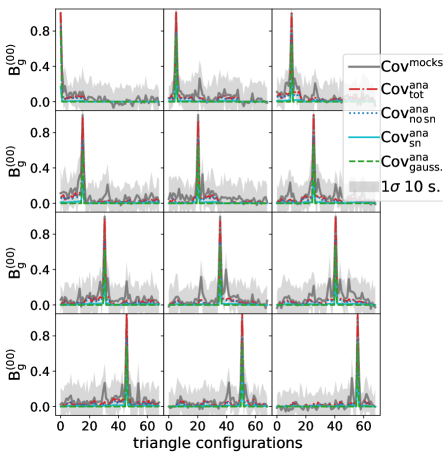
Figure 2: Columns of the reduced covariance matrices, both analytical and numerical. The shaded area is obtained by randomly splitting the 1400 mocks in 10 groups, obtaining the numerical covariance matrix for each of them (correcting by the appropriate Hartlap factor) and finally computing each covariance matrix element standard deviation. In the left panel is shown the comparison for the bispectrum auto-covariance matrix while on the right for its cross-correlation with each of the power spectrum multipoles modes. The different lines shows the contributions given by the Gaussian term, the shot-noise correction and the non-Gaussian contribution.
Refer to caption
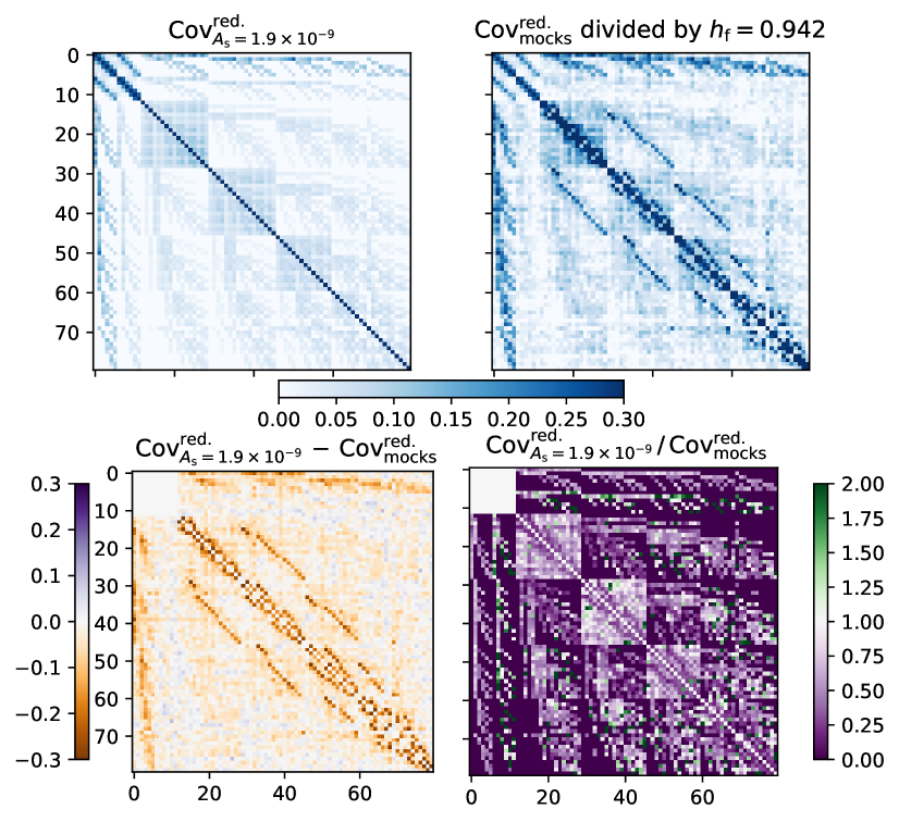
Figure 3: Reduced analytical (top-left) and numerical (top-right) covariance matrices for the [Pg(0,2);Bg(00)]superscriptsubscriptPg02superscriptsubscriptBg00\mathrm{\left[\mathrm{P}_{\mathrm{g}}^{(0,2)};\mathrm{B}_{\mathrm{g}}^{(00)}\right]} data vector, Δk5Δsubscript𝑘5\Delta k_{5} case. In the bottom row are also shown the difference (left) and ratio (right) between the two covariance matrices. In order to minimise the potential systematics given by analytically model the covariance matrix, we used the auto-covariance of the power spectrum multipoles estimated from the mocks also in our analytical (hybrid) covariance. That is the reason why in the above Figure there is no difference between analytical and numerical covariances for Pg(0,2)superscriptsubscriptPg02\mathrm{P}_{\mathrm{g}}^{(0,2)}. From the bottom row we can see that the analytical model misses certain features close to the diagonal for the bispectrum auto-covariance. In the cross correlation part, the cross correlation between power spectrum monopole and bispectrum monopole is slightly underestimated while the one with the power spectrum quadrupole is slightly overestimated.

5 Numerical and hybrid covariance matrix for [𝐏𝐠(𝟎,𝟐);𝐁𝐠(𝟎𝟎)]superscriptsubscript𝐏𝐠02superscriptsubscript𝐁𝐠00\mathbf{\left[{P}_{g}^{(0,2)};{B}_{g}^{(00)}\right]}

We compare the analytical covariance matrix for the data vector [Pg(0,2);Bg(00)]superscriptsubscriptPg02superscriptsubscriptBg00\mathrm{\left[\mathrm{P}_{\mathrm{g}}^{(0,2)};\mathrm{B}_{\mathrm{g}}^{(00)}\right]} with a numerical one derived by measuring the above statistics from 1400 realisations of the MultiDark Patchy BOSS DR12 galaxy catalogues [61, 74]. The Patchy mocks reproduce the number density, selection function, survey geometry and clustering properties of BOSS DR12 galaxy sample [4]; for each mock the power spectrum monopole and quadrupole are available and we have calculated the bispectrum monopole for both North and South Galactic Caps (NGC and SGC).

The same fiducial cosmology of the mocks, ΩΛ=0.693subscriptΩΛ0.693\Omega_{\Lambda}=0.693, Ωm(z=0)=0.307subscriptΩm𝑧00.307\Omega_{\mathrm{m}}(z=0)=0.307, Ωb(z=0)=0.048subscriptΩb𝑧00.048\Omega_{\mathrm{b}}(z=0)=0.048, σ8(z=0)=0.829subscript𝜎8𝑧00.829\sigma_{8}(z=0)=0.829, ns=0.96subscript𝑛s0.96n_{\mathrm{s}}=0.96, h0=0.678subscript00.678h_{0}=0.678, has been used the generate the necessary analytical matter power spectrum [63] for our modeling.

Note that the covariance matrix obtained from the survey mocks has a contribution due to the survey window function. The analytic expression for the covariance matrix does not account for the extra mode-coupling and thus coupling between different statistics, induced by the window. In our analytically-generated data vector used for parameter forecast we do not include the survey window effect, hence we do not worry too much about modeling the same effect in the covariance matrix. More discussion on the effect of the window can be found below and in Appendix C. In order to model the window additional contribution to statistical error one could proceed as in [53] for the CMB angular power spectrum: under the assumption of the mask correction being small with respect to the signal covariance, the total covariance could be written as a sum Ctot=Csignal+CmasksubscriptCtotsubscriptCsignalsubscriptCmask\mathrm{C_{tot}}=\mathrm{C_{signal}}+\mathrm{C_{mask}}.

Similarly to [88] we set the bias parameters values b1=2.0subscript𝑏12.0b_{1}=2.0 and b2=0.subscript𝑏20b_{2}=0., together with using the same effective survey volume Vs=1.76[h1Gpc]3subscript𝑉s1.76superscriptdelimited-[]superscript1Gpc3V_{\mathrm{s}}=1.76\left[h^{-1}\,\mathrm{Gpc}\right]^{3}. The choice for the linear bias b1subscript𝑏1b_{1} is not too dissimilar from what obtained in the BOSS clustering analysis [44] while the survey volume derived in [88] is not too far from the one (Vs=1.92[h1Gpc]3subscript𝑉s1.92superscriptdelimited-[]superscript1Gpc3V_{\mathrm{s}}=1.92\left[h^{-1}\,\mathrm{Gpc}\right]^{3}) fitted from comparing the numerical covariance estimated from the mocks and its theoretical model in the 3-pt correlation function analysis done in [87].
Refer to caption
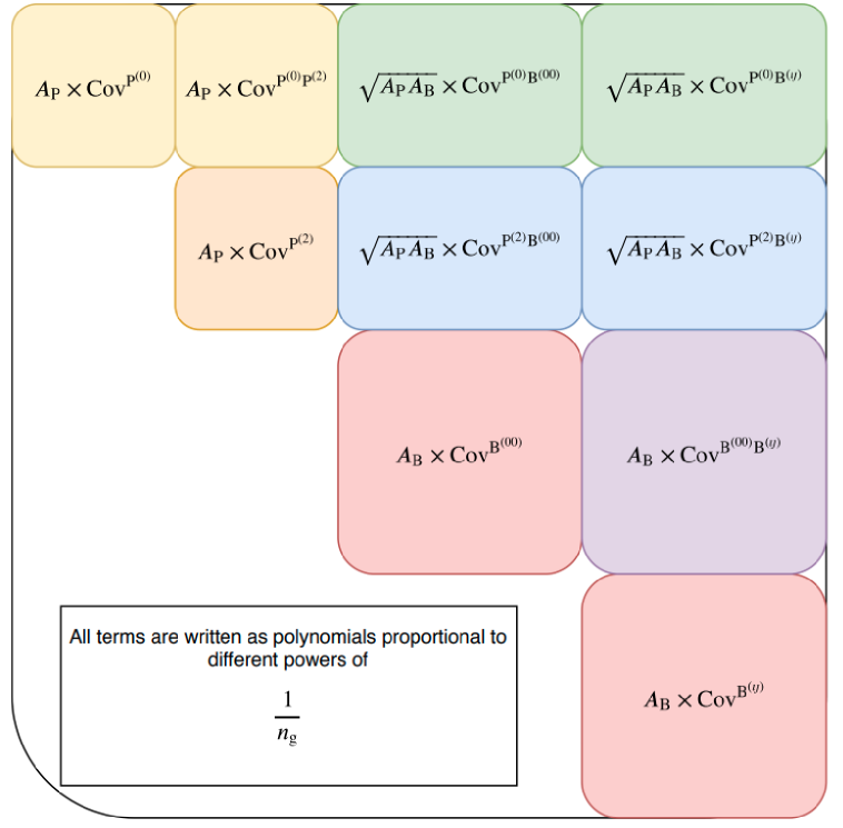
Figure 4: Analytical covariance matrix: calibrated terms. The powers of the average galaxy number density enter the different components of the data vector’s covariance as shown in Equation 5.1. From this figure we can see the difference between fitting the two power spectrum and bispectrum covariance amplitude parameters APsubscript𝐴PA_{\mathrm{P}}, ABsubscript𝐴BA_{\mathrm{B}} and the physical scalar perturbation amplitude parameter Assubscript𝐴sA_{\mathrm{s}}. The power spectrum part of the covariance is proportional to As2superscriptsubscript𝐴s2A_{\mathrm{s}}^{2} (Gaussian term, Equation 4.2 ), the bispectrum part to both As3superscriptsubscript𝐴s3A_{\mathrm{s}}^{3} (Gaussian term, Equation 4) and to As4superscriptsubscript𝐴s4A_{\mathrm{s}}^{4} (non-Gaussian term, Equations 4 and 4); the cross-covariance terms are proportional to As3superscriptsubscript𝐴s3A_{\mathrm{s}}^{3} (Equation 4). To calibrate Assubscript𝐴sA_{\mathrm{s}} would then imply changing not only the balance between different parts of the covariance but also, as for the case of the bispectrum, the balance between Gaussian and non-Gaussian contributions belonging to the same terms. This is the reason why we prefer to estimate a priori through an MCMC sampling an effective value of Assubscript𝐴sA_{\mathrm{s}}. Only afterwards, after the analytical covariance expressions have been computed, we calibrate the two parameters APsubscript𝐴PA_{\mathrm{P}}, ABsubscript𝐴BA_{\mathrm{B}}. These can be interpreted as corrections to the analytically computed Fourier integration volume for each covariance matrix component.

In the power spectrum multipoles covariance matrix expression we set Δk=0.01h/\Delta k=0.01h/Mpc, which is the same value used in numerical measurement pipeline. For the galaxy bispectrum we use two different ΔkΔ𝑘\Delta k bin sizes proportional to the fundamental frequency kf=(2π)3Vbsubscript𝑘𝑓superscript2𝜋3subscript𝑉bk_{f}=\frac{(2\pi)^{3}}{V_{\mathrm{b}}} where Vb=(3500Mpc/h)3subscript𝑉bsuperscript3500Mpc3V_{\mathrm{b}}=(3500\,\mathrm{Mpc}/h)^{3} is the survey volume for the mock catalogues cubic box. We select the two cases: Δk6,5=6,5×kfΔsubscript𝑘6565subscript𝑘𝑓\Delta k_{6,5}=6,5\times k_{f} which given our algorithm [44] to generate (k1,k2,k3)subscript𝑘1subscript𝑘2subscript𝑘3(k_{1},k_{2},k_{3}) triplets imposing the triangle closure condition and the range of scales considered, corresponds to using 32 and 68 triangle configurations, respectively. In the main body of this work all the results for the Δk5Δsubscript𝑘5\Delta k_{5} case have been presented. The key figures and table for the Δk6Δsubscript𝑘6\Delta k_{6} case are shown in Appendix D.

We adopt a very conservative k𝑘k-range for the sides of the triangle configurations used for the bispectrum multipoles, in particular we set kmin=0.03hsubscript𝑘min0.03k_{\mathrm{min}}=0.03\,h/Mpc and kmax=0.09hsubscript𝑘max0.09k_{\mathrm{max}}=0.09\,h/Mpc. The reason for choosing a low kmaxsubscript𝑘maxk_{\mathrm{max}} is twofold. Firstly, this allows us to trust our standard perturbation theory calculations at tree-level, for example for what concerns the cross-correlation between power spectrum and bispectrum as noted in [88]. Secondly, this choice limits the number of triangle configurations in the data vector. This is essential in order to make it feasible to analytically compute in a reasonable amount of time all the terms of the covariance matrix with a sufficient precision. Moreover, the longer the data vector, the less numerically stable is the inversion of its covariance matrix needed for the likelihood evaluation. As already pointed out in [47] this is the case when several multipoles of the bispectrum are present simultaneously in the data vector without compression.

Nevertheless by choosing kmax=0.09hsubscript𝑘max0.09k_{\mathrm{max}}=0.09\,h/Mpc our analysis uses only a fraction of the baryonic acoustic oscillations information encoded in the galaxy density field. To fully capture and exploit this information and in particular its anisotropic component using the bispectrum multipoles, it would be necessary to further improve the covariance analytical model to extend its reliability to higher k𝑘k’s. For this reason our finding might be conservative.

In order to choose the scalar amplitude parameter Assubscript𝐴sA_{\mathrm{s}} needed to compute the linear matter power spectrum (with CLASS [63]) to be used in the analytical covariance matrix template, we run a preliminary MCMC sampling using the numerical covariance matrix and the mean of the mocks as data vector. We then leave Assubscript𝐴sA_{\mathrm{s}} free to vary together with the additional parameters (b1,b2,f,α,α)subscript𝑏1subscript𝑏2𝑓subscript𝛼perpendicular-tosubscript𝛼parallel-to(b_{1},b_{2},f,\alpha_{\perp},\alpha_{\parallel}). We obtain As1.9×109similar-to-or-equalssubscript𝐴s1.9superscript109A_{\mathrm{s}}\simeq 1.9\times 10^{-9} as a best-fit value, we recognize that this is lower than the value reported in the Planck analysis [1] (As=3.04×10⁹subscript𝐴s3.04superscript109A_{\mathrm{s}}=3.04\times 10^{-9}). This is just a shortcut to make our calculations numerically stable. In fact, as reported below, and explained in Fig. 4 the effective amplitude of the power spectrum and bispectrum covariances are later free parameters of the normalisation.

For the covariance computation we set the FoG parameters in Equation 3 for the power spectrum and bispectrum multipoles to the best fit values obtained in the BOSS analysis [44], σP=3.5subscript𝜎P3.5\sigma_{\mathrm{P}}=3.5 and σB=7.39subscript𝜎B7.39\sigma_{\mathrm{B}}=7.39. In fact, even if we limit our k𝑘k-range to linear scales where the FoG effect should be negligible, in some of the covariance matrix terms (in particular, shot-noise correction terms) the sums of two or three k𝑘k-vectors appear in the argument of the power spectrum or bispectrum. This is not the case for the terms proportional to the trispectrum and hence no FoG parameter is used for the trispectrum. In the data vector’s model used for the MCMC samplings both σPsubscript𝜎P\sigma_{\mathrm{P}} and σBsubscript𝜎B\sigma_{\mathrm{B}} have been set to zero since we limit our analysis to linear scales.

To calibrate the covariance matrix we adjust three parameters: the average number density of galaxies ngsubscript𝑛gn_{\mathrm{g}}, an effective amplitude for the power spectrum part of the covariance APsubscript𝐴PA_{\mathrm{P}} and another effective amplitude ABsubscript𝐴BA_{\mathrm{B}} for the bispectrum part. These parameters act on the calibrated terms as shown in Figure 4. Figure 4 clarifies the difference between fitting the two amplitude parameters APsubscript𝐴PA_{\mathrm{P}}, ABsubscript𝐴BA_{\mathrm{B}} and the physical scalar amplitude Assubscript𝐴sA_{\mathrm{s}}. While Assubscript𝐴sA_{\mathrm{s}} is common to all the terms in the covariance, each is term proportional to a different power of the scalar perturbations amplitude parameter (see caption of Figure 4 for details), APsubscript𝐴PA_{\mathrm{P}} and ABsubscript𝐴BA_{\mathrm{B}} can be interpreted as separate corrections to the analytically-computed integration volumes in Fourier space for power spectrum (Vp=4πΔkk2subscript𝑉p4𝜋Δ𝑘superscript𝑘2V_{\mathrm{p}}=4\pi\Delta kk^{2}) and bispectrum (V123t=8π2k1k2k3Δk1Δk2Δk3subscriptsuperscript𝑉t1238superscript𝜋2subscript𝑘1subscript𝑘2subscript𝑘3Δsubscript𝑘1Δsubscript𝑘2Δsubscript𝑘3V^{\mathrm{t}}_{123}=8\pi^{2}k_{1}k_{2}k_{3}\Delta k_{1}\Delta k_{2}\Delta k_{3}). The analytical expressions for these volumes, which are used to normalise the statistics estimators by the number of modes measured (see Appendix A of [48] for a detailed explanation), are obtained in the "infinitesimal" bin-width approximation. In particular using Δk=5,6×kfsubscriptΔ𝑘56subscript𝑘f\Delta_{k}=5,6\times k_{\mathrm{f}} and limiting our analysis to small k𝑘k’s the condition kΔkmuch-less-than𝑘subscriptΔ𝑘k\ll\Delta_{k} may not be optimal. Moreover, APsubscript𝐴PA_{\mathrm{P}}, ABsubscript𝐴BA_{\mathrm{B}} can also account for a mismatch between the fiducial effective survey volume value and the real one. Therefore it is not surprising that a calibration of these quantities is needed when they are not measured but computed analytically; reassuringly, their value is of the order of unity as reported in Table 1.

For what concerns ngsubscript𝑛gn_{\mathrm{g}}, we treat it as a free parameter in order to model shot-noise deviations from Poissonian behaviour. This is non uncommon and often also used when analyzing galaxy surveys. Indeed the expressions that we use to account for the shot-noise terms in the covariance model were derived under the Poissonian approximation (see Ref. [88]). Even letting ngsubscript𝑛gn_{\mathrm{g}} free to vary, we find a best fit value very similar to the one computed in Ref. [88] for the same data-set.

We fit these parameters by comparing the diagonal of the analytical covariance matrix with the one numerically estimated using a set of 1400 Patchy galaxy mock catalogue realisations after correction by the Hartlap factor hf=(NmocksNdv2)/(Nmocks1)subscriptfsubscript𝑁mockssubscript𝑁dv2subscript𝑁mocks1h_{\mathrm{f}}=(N_{\mathrm{mocks}}-N_{\mathrm{dv}}-2)/(N_{\mathrm{mocks}}-1) [51], where Ndvsubscript𝑁dvN_{\mathrm{dv}} is the data vector’s size while Nmockssubscript𝑁mocksN_{\mathrm{mocks}} is the number of galaxy catalogues used to estimate the covariance (1400 in our case). In summary calibration is done following the expression below:

CtotP(),B(ı,ȷ)={AP×[CPng0+1ngCPng1+1ng2CPng2],for Pg() cov.AB×[CBıȷng0+1ngCBıȷng1+1ng2CBıȷng2+1ng3CBıȷng3+1ng4CBıȷng4],for Bg(ıȷ) cov.APAB×[CPg()Bıȷng0+1ngCPg()Bıȷng1+1ng2CPg()Bıȷng2+1ng3CPg()Bıȷng3],for Pg()Bg(ıȷ) cross-cov.superscriptsubscript𝐶totsuperscriptPsuperscriptBitalic-ıitalic-ȷcasessubscript𝐴Pdelimited-[]superscriptsubscript𝐶superscriptPsuperscriptsubscript𝑛g01subscript𝑛gsuperscriptsubscript𝐶superscriptPsuperscriptsubscript𝑛g11superscriptsubscript𝑛g2superscriptsubscript𝐶superscriptPsuperscriptsubscript𝑛g2for subscriptsuperscriptPg cov.subscript𝐴Bdelimited-[]superscriptsubscript𝐶superscriptBitalic-ıitalic-ȷsuperscriptsubscript𝑛g01subscript𝑛gsuperscriptsubscript𝐶superscriptBitalic-ıitalic-ȷsuperscriptsubscript𝑛g11superscriptsubscript𝑛g2superscriptsubscript𝐶superscriptBitalic-ıitalic-ȷsuperscriptsubscript𝑛g21superscriptsubscript𝑛g3superscriptsubscript𝐶superscriptBitalic-ıitalic-ȷsuperscriptsubscript𝑛g31superscriptsubscript𝑛g4superscriptsubscript𝐶superscriptBitalic-ıitalic-ȷsuperscriptsubscript𝑛g4for subscriptsuperscriptBitalic-ıitalic-ȷg cov.subscript𝐴Psubscript𝐴Bdelimited-[]superscriptsubscript𝐶subscriptsuperscriptPgsuperscriptBitalic-ıitalic-ȷsuperscriptsubscript𝑛g01subscript𝑛gsuperscriptsubscript𝐶subscriptsuperscriptPgsuperscriptBitalic-ıitalic-ȷsuperscriptsubscript𝑛g11superscriptsubscript𝑛g2superscriptsubscript𝐶subscriptsuperscriptPgsuperscriptBitalic-ıitalic-ȷsuperscriptsubscript𝑛g21superscriptsubscript𝑛g3superscriptsubscript𝐶subscriptsuperscriptPgsuperscriptBitalic-ıitalic-ȷsuperscriptsubscript𝑛g3for subscriptsuperscriptPgsubscriptsuperscriptBitalic-ıitalic-ȷg cross-cov.\displaystyle C_{\mathrm{tot}}^{\mathrm{P}^{(\ell)},\mathrm{B}^{(\imath,\jmath)}}=\begin{cases}A_{\mathrm{P}}\times\left[C_{\mathrm{P}^{\ell}}^{n_{\mathrm{g}}^{0}}+\dfrac{1}{n_{\mathrm{g}}}C_{\mathrm{P}^{\ell}}^{n_{\mathrm{g}}^{-1}}+\dfrac{1}{n_{\mathrm{g}}^{2}}C_{\mathrm{P}^{\ell}}^{n_{\mathrm{g}}^{-2}}\right],&\mbox{for }\mathrm{P}^{(\ell)}_{\mathrm{g}}\mbox{ cov.}\\ A_{\mathrm{B}}\times\left[C_{\mathrm{B}^{\imath\jmath}}^{n_{\mathrm{g}}^{0}}+\dfrac{1}{n_{\mathrm{g}}}C_{\mathrm{B}^{\imath\jmath}}^{n_{\mathrm{g}}^{-1}}+\dfrac{1}{n_{\mathrm{g}}^{2}}C_{\mathrm{B}^{\imath\jmath}}^{n_{\mathrm{g}}^{-2}}+\dfrac{1}{n_{\mathrm{g}}^{3}}C_{\mathrm{B}^{\imath\jmath}}^{n_{\mathrm{g}}^{-3}}+\dfrac{1}{n_{\mathrm{g}}^{4}}C_{\mathrm{B}^{\imath\jmath}}^{n_{\mathrm{g}}^{-4}}\right],&\mbox{for }\mathrm{B}^{(\imath\jmath)}_{\mathrm{g}}\mbox{ cov.}\\ \sqrt{A_{\mathrm{P}}A_{\mathrm{B}}}\times\left[C_{\mathrm{P}^{(\ell)}_{\mathrm{g}}\mathrm{B}^{\imath\jmath}}^{n_{\mathrm{g}}^{0}}+\dfrac{1}{n_{\mathrm{g}}}C_{\mathrm{P}^{(\ell)}_{\mathrm{g}}\mathrm{B}^{\imath\jmath}}^{n_{\mathrm{g}}^{-1}}+\dfrac{1}{n_{\mathrm{g}}^{2}}C_{\mathrm{P}^{(\ell)}_{\mathrm{g}}\mathrm{B}^{\imath\jmath}}^{n_{\mathrm{g}}^{-2}}+\dfrac{1}{n_{\mathrm{g}}^{3}}C_{\mathrm{P}^{(\ell)}_{\mathrm{g}}\mathrm{B}^{\imath\jmath}}^{n_{\mathrm{g}}^{-3}}\right],&\mbox{for }\mathrm{P}^{(\ell)}_{\mathrm{g}}\mathrm{B}^{(\imath\jmath)}_{\mathrm{g}}\mbox{ cross-cov.}\end{cases} (5.1)

In Table 1 are reported the values for the fitted parameters both in the Δk5Δsubscript𝑘5\Delta k_{5} and Δk6Δsubscript𝑘6\Delta k_{6} cases.

k𝑘k-bin size Ntr.subscript𝑁trN_{\mathrm{tr.}} APsubscript𝐴PA_{\mathrm{P}} ABsubscript𝐴BA_{\mathrm{B}} ng[h/Mpc]3subscript𝑛gsuperscriptdelimited-[]Mpc3n_{\mathrm{g}}\;\left[h/\mathrm{Mpc}\right]^{3} Rc=Covana.ii/Covnum.iisubscriptRcdelimited-⟨⟩superscriptsubscriptCovanaiisuperscriptsubscriptCovnumii\mathrm{R_{c}}=\langle\mathrm{Cov_{ana.}^{ii}}/\mathrm{Cov_{num.}^{ii}}\rangle σ(Rc)𝜎subscriptRc\sigma\left(\mathrm{R_{c}}\right)
Δk6Δsubscript𝑘6\Delta k_{6} 32 1.457 1.024 3.49 ×10⁴absentsuperscript104\times 10^{-4} 0.997 0.057
Δk5Δsubscript𝑘5\Delta k_{5} 68 1.480 0.868 3.25 ×10⁴absentsuperscript104\times 10^{-4} 0.998 0.047
Table 1: Values for the analytic covariance matrix parameters fitted by comparing the diagonal elements with those obtained numerically from the mock catalogues. On the last two columns are shown the average and the standard deviation relative to the ratio between the analytical and numerical covariance matrices diagonals. The fitted values of ngsubscript𝑛gn_{\mathrm{g}} are very close, especially in the Δk5Δsubscript𝑘5\Delta k_{5} case, to the one computed in [88].
Refer to caption
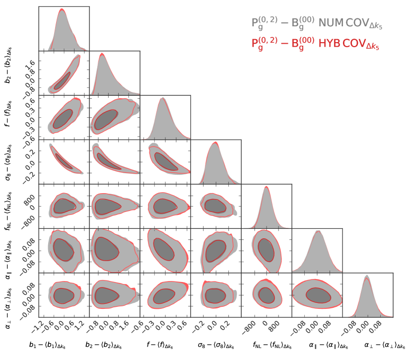
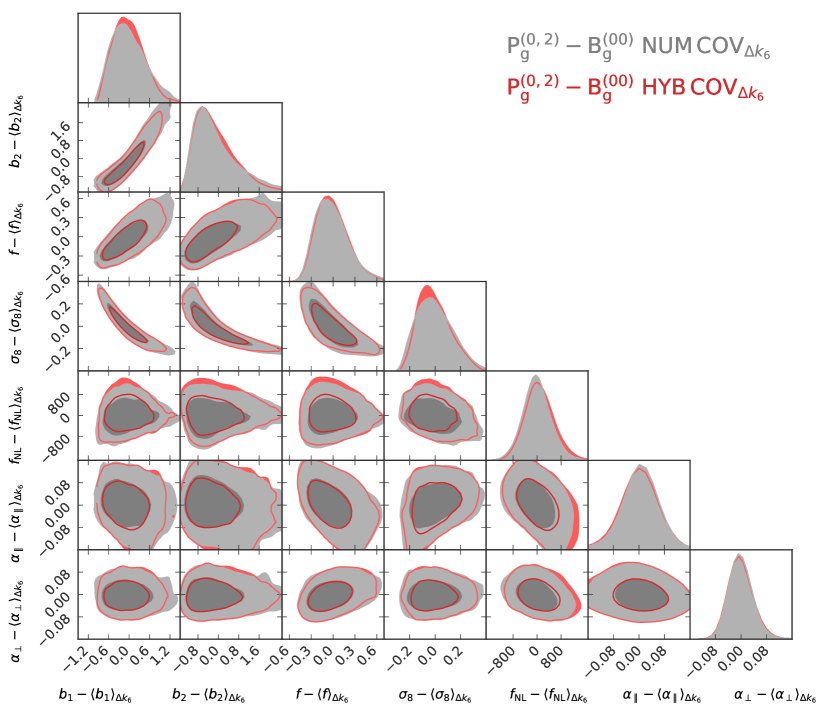
Figure 5: 1 and 2D marginalised posterior distributions for the data vector [Pg(0,2);Bg(00)]superscriptsubscriptPg02superscriptsubscriptBg00\mathrm{\left[\mathrm{P}_{\mathrm{g}}^{(0,2)};\mathrm{B}_{\mathrm{g}}^{(00)}\right]}, Δk5Δsubscript𝑘5\Delta k_{5} case. In gray (NUM COV) are shown the posterior contours given by employing the numerical covariance matrix estimated from the mocks to evaluate the likelihood, while in red (HYB COV) the equivalent is shown for the case in which the analytic/hybrid covariance has been used for the same purpose. Both 1-2D, 68%percent\% and 95%percent\% confidence intervals show good agreement with no significant difference in terms of the shape of the degeneracies present between the different parameters.

5.1 Visual comparison

We begin by visually inspecting the differences between the analytical covariance matrix (after calibration) and the numerical. Figure 2 shows 1D sections (columns/rows) for both the bispectrum autocovariance and its cross-correlation with the power spectrum for the Δk5Δsubscript𝑘5\Delta k_{5} case. The shaded area is obtained by splitting the 1400 mocks into ten groups and then computing the numerical covariance matrix for each of them. From the ten estimated covariance matrices we compute each element’s standard deviation as a proxy for the statistical noise. This gives us a possible estimate of the level of agreement between analytical and numerical covariance matrices. The bispectrum auto-covariance results are well approximated (mostly within the shaded area) by the analytical model.

The cross-covariance between bispectrum and power spectrum multipoles shows a larger discrepancy between numerical and analytical covariance matrices. In particular the amplitude of certain elements seems to be lower in the analytical case. For other "pixels" the analytical value is exactly equal to zero due to the Kronecker’s delta condition from Equation 4. The absence in our model of higher order terms such as the one proportional to the tetraspectrum could explain the lower amplitude observed in the analytical lines in the right panel of Figure 2. In the pixels where the analytical covariance matrix is by definition equal to zero we see that the shaded area indicates that also the numerical estimate is compatible with zero and therefore the non-null values seen in the numerical covariance matrix could be interpreted simply as statistical noise. Another source of discrepancy could be the lack of the survey window selection effect in our covariance template (more below). Finally the shot-noise correction appears to be relatively negligible with respect to the non-Gaussian terms for the off-diagonal elements.

It also results useful to look at the whole 2D analytical and numerical reduced covariance matrices (i.e., element of row i and column j is divided by the square root of the product of element ii times element jj). In Figure 3 are shown the reduced covariance matrices for the Δk5Δsubscript𝑘5\Delta k_{5} binning case333Another reason to choose this binning case for the whole analysis is that there are enough triangle configurations to resolve the structure and features present in the covariance matrix but not too many to make them invisible due to the limited size of the image.. The comparison between the numerical and analytical covariance reveals qualitative good agreement. The only relevant difference is the lack, in the calibrated hybrid template, of the features parallel to the covariance diagonal. These features are due to the additional mode-coupling induced by the survey window. In Appendix C we compare our hybrid model to the numerical covariance obtained from a set of 440 simulated galaxy fields in cubic boxes with periodic boundary conditions [27]. In Figure 13 we see that in the absence of survey mask and window, such features are not present in the covariance matrix. It will become evident in Section 5.2 that these features have no significant effect on our analysis.

Refer to caption
Figure 6: Relative difference between analytical and numerical covariance matrix results for what concerns the 1D 68%percent\% confidence intervals and median values obtained from running a MCMC sampling using as data vector each measurement of [Pg(0,2);Bg(00)]superscriptsubscriptPg02superscriptsubscriptBg00\mathrm{\left[\mathrm{P}_{\mathrm{g}}^{(0,2)};\mathrm{B}_{\mathrm{g}}^{(00)}\right]} from the 1400 mock catalogues. The horizontal lines inside the violins delimitate the central quartiles of the ratios distribution. From the violin plots above it is possible to infer that, for the vast majority of the mocks, the difference between the values obtained using the analytical and numerical covariance matrices is less than 25%percent2525\% the value of the 1D 68%percent\% confidence intervals obtained using the numerical covariance matrix.
Refer to caption
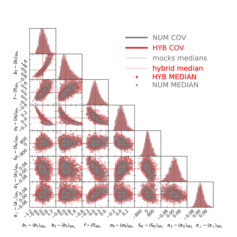
Figure 7: Cosmological parameters posterior distributions for [Pg(0,2);Bg(00)]superscriptsubscriptPg02superscriptsubscriptBg00\mathrm{\left[\mathrm{P}_{\mathrm{g}}^{(0,2)};\mathrm{B}_{\mathrm{g}}^{(00)}\right]} data vector, Δk5Δsubscript𝑘5\Delta k_{5} case. In gray (MOCKS COV) and red (HYB COV) are shown the 1-2D marginalised posterior distributions for using as data vector the mean of the mocks together with the numerical and hybrid covariance matrices to evaluate the likelihood, respectively. On top of these contours we show the scatter of the median values for all the model parameters obtained for each of the 1400 galaxy catalogues, again using both numerical and hybrid covariance matrices. The similarity of the posteriors and the scatter among the mocks adds further confidence in the reliability of our fitted analytical model of the data vector’s covariance.

5.2 Constraints comparison for the (reduced) data vector [𝐏𝐠(𝟎,𝟐);𝐁𝐠(𝟎𝟎)]superscriptsubscript𝐏𝐠02superscriptsubscript𝐁𝐠00\mathbf{\left[P_{g}^{(0,2)};B_{g}^{(00)}\right]}

We estimate the cosmological posterior for the (reduced) data vector [𝐏𝐠(𝟎,𝟐);𝐁𝐠(𝟎𝟎)]superscriptsubscript𝐏𝐠02superscriptsubscript𝐁𝐠00\mathbf{\left[P_{g}^{(0,2)};B_{g}^{(00)}\right]} using the analytical/hybrid covariance matrix and the numerical one. Whenever we compare the two covariance matrices we use for each test the same data vector. In this section we either use the mean measurement from the mocks or each individual mock measurement.

To compare the two posteriors so obtained, we consider a seven parameters set:
(b1,b2,f,σ8,fNL,α,α)subscript𝑏1subscript𝑏2𝑓subscript𝜎8subscript𝑓NLsubscript𝛼perpendicular-tosubscript𝛼parallel-to(b_{1},b_{2},f,\sigma_{8},f_{\mathrm{NL}},\alpha_{\perp},\alpha_{\parallel}), where b1subscript𝑏1b_{1} and b2subscript𝑏2b_{2} are the first and second order Eulerian bias parameters, f𝑓f is the linear growth-rate, σ8subscript𝜎8\sigma_{8} is the normalisation of the matter power spectrum, fNLsubscript𝑓NLf_{\mathrm{NL}} is the amplitude of local primordial non-Gaussianity perturbations [93, 62, 10, 20] and αsubscript𝛼perpendicular-to\alpha_{\perp}, αsubscript𝛼parallel-to\alpha_{\parallel} are the Alcock-Paczyǹsky parameters.

Following what is done in the BOSS analyses [43, 44] we use the local Lagrangian bias approximation to fix the value of the non-local tidal bias parameter bs2subscript𝑏subscripts2b_{\mathrm{s}_{2}} appearing in the second order kernel of the bispectrum to bs2=4(b11)/7subscript𝑏subscripts24subscript𝑏117b_{\mathrm{s}_{2}}=-4(b_{1}-1)/7. We have checked through a specific MCMC sampling that allowing this parameter to vary does not significantly change our results.

This is shown in Figure 5 for the Δk5Δsubscript𝑘5\Delta k_{5} case (for which there are 68 triangle configurations in the bispectrum data vector).

Since we focus on the change in the parameter constraints width, we show our results with each parameter’s central value (median) subtracted. The central value is given by the analysis performed using the numerical covariance matrix. A full parameters constraints analysis will be presented elsewhere.

From Figure 5 we can see that qualitatively there is very good agreement between the posterior distributions obtained with the hybrid and numerical covariance matrices. With another separate MCMC run we tested what happens in both cases: setting to zero all the off-diagonal terms or only the bispectrum auto-covariance ones. The resulting marginalised 1-2D posterior distributions are- not unexpetedly- significantly tighter then the ones obtained using the covariance matrix estimated from the mocks.

We go even further to quantify the performance of the hybrid covariance matrix approach: we perform a MCMC sampling on the data vector measurement from each of 1400 mock catalogues using both analytic and the hybrid covariance matrices.

We then compare in Figure 6 the probability distributions 1D 68%percent\% confidence intervals and the medians for each model parameter. The relative difference between variances and medians obtained using numerical and hybrid covariances is for the large majority of the mocks less than 25%similar-toabsentpercent25\sim 25\% the value of each parameter’s variance. In Figure 7 we show the 1 and 2D posterior distributions for the parameters and the scatter of the median444As it is common to do in Bayesian inference, we stick to the so-called Central Credible Interval which reports errors around the median of a distribution. Posteriors are very symmetric hence the median is very close to the mean and the maximum anyway. values for each mock realisation. Point and lines in red correspond to the analytic/hybrid covariance, points and lines in gray correspond to the numerical covariance.

From these quantitative and statistical tests we conclude that our analytical model, once calibrated (i.e., fitting the three parameters AP,AB,ngsubscript𝐴Psubscript𝐴Bsubscript𝑛gA_{\mathrm{P}},\,A_{\mathrm{B}},\,n_{\mathrm{g}}), represents a realistic proxy for the covariance matrix estimated from the galaxy mock catalogues for the [Pg(0,2);Bg(00)]superscriptsubscriptPg02superscriptsubscriptBg00\mathrm{\left[\mathrm{P}_{\mathrm{g}}^{(0,2)};\mathrm{B}_{\mathrm{g}}^{(00)}\right]} data vector.

Given this result, the main assumption of this work is to consider reliable the extension of our covariance model to the galaxy bispectrum higher multipoles. This is motivated by the fact that our choice of fitting parameters does not depend on the multipole chosen but just on the statistic (power spectrum or bispectrum).

6 Higher multipoles of the bispectrum: 𝐁𝐠(𝟐𝟎),𝐁𝐠(𝟎𝟐),𝐁𝐠(𝟒𝟎),𝐁𝐠(𝟎𝟒),𝐁𝐠(𝟐𝟐)superscriptsubscript𝐁𝐠20superscriptsubscript𝐁𝐠02superscriptsubscript𝐁𝐠40superscriptsubscript𝐁𝐠04superscriptsubscript𝐁𝐠22\mathbf{B_{g}^{(20)},B_{g}^{(02)},B_{g}^{(40)},B_{g}^{(04)},B_{g}^{(22)}}

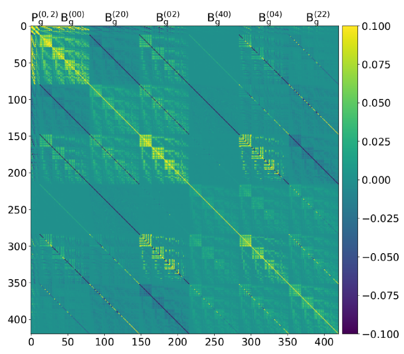
We now proceed to estimate the added value given by extending the clustering statistics data vector to the galaxy bispectrum higher multipoles. We use the covariance analytical model presented in Section 4 to sample the model parameters posterior distribution. In Figure 8 the resulting reduced covariance matrix for the data vector [Pg(0,2);Bg(00,20,02,40,04,22)]superscriptsubscriptPg02subscriptsuperscript𝐵002002400422𝑔\left[\mathrm{P_{g}^{(0,2)}};B^{(00,20,02,40,04,22)}_{g}\right] is displayed. As an example it is interesting to notice that bispectrum monopole Bg(00)superscriptsubscriptBg00\mathrm{B_{g}^{(00)}} is negatively correlated with Bg(20)superscriptsubscriptBg20\mathrm{B_{g}^{(20)}} while positively correlated with Bg(02)superscriptsubscriptBg02\mathrm{B_{g}^{(02)}}. The difference in the correlations between different bispectrum multipoles terms suggests that the multipoles have complementary constraining power.
Refer to caption
Figure 8: Reduced covariance matrix for the data vector including the galaxy bispectrum higher multipoles, [Pg(0,2);Bg(00,20,02,40,04,22)]superscriptsubscriptPg02superscriptsubscriptBg002002400422\mathrm{\left[\mathrm{P}_{\mathrm{g}}^{(0,2)};\mathrm{B}_{\mathrm{g}}^{(00,20,02,40,04,22)}\right]}, for the Δk5Δsubscript𝑘5\Delta k_{5} case. It is interesting to notice the different sign of the correlation between the bispectrum multipoles. For example Bg(00)superscriptsubscriptBg00\mathrm{B}_{\mathrm{g}}^{(00)} and Bg(20)superscriptsubscriptBg20\mathrm{B}_{\mathrm{g}}^{(20)} are anti-correlated in the off-diagonal terms whilst Bg(00)superscriptsubscriptBg00\mathrm{B}_{\mathrm{g}}^{(00)} and Bg(02)superscriptsubscriptBg02\mathrm{B}_{\mathrm{g}}^{(02)} are positively correlated. This information hints to the additional constraining power achievable through the employment of both Bg(20)superscriptsubscriptBg20\mathrm{B}_{\mathrm{g}}^{(20)} and Bg(02)superscriptsubscriptBg02\mathrm{B}_{\mathrm{g}}^{(02)} since they are differently correlated to the isotropic signal, Bg(00)superscriptsubscriptBg00\mathrm{B}_{\mathrm{g}}^{(00)}.
Refer to caption
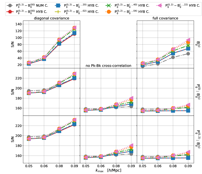
Figure 9: Comulative signal to noise ratio as a function of kmaxsubscript𝑘maxk_{\mathrm{max}} for the different statistics computed using an analytical model for the data vector and both the analytical and numerical covariance matrices, computed using Equation 6.1. In the first row are displayed the lines for the signal to noise ratio when only the bispectrum multipoles are employed. In the second and third rows the power spectrum monopole and quadrupole are added to the data vector, respectively. In the first column only the diagonals of the covariance matrices (uncorrelated data vector’s elements) have been used in the cumulative signal to noise ratio computation. In the second column we set to zero the cross-correlation between power spectrum and bispectrum multipoles, leaving the off-diagonal terms in the auto-covariances. Finally in the third column we employed the full covariance matrices to compute the signal to noise ratio. From the plot it appears that in terms of cumulative signal to noise the saturation is reached when both the hexadecapole terms of the galaxy bispectrum are included in the data vector. The discrepancy between the [Pg(0,2);Bg(00)]superscriptsubscriptPg02superscriptsubscriptBg00\mathrm{\left[\mathrm{P}_{\mathrm{g}}^{(0,2)};\mathrm{B}_{\mathrm{g}}^{(00)}\right]} lines for numerical and analytical covariance matrices is clearly due to the cross-covariance term between power spectrum and bispectrum multipoles. A possible explanation is the lack of higher order terms in the cross-covariance and the presence of many elements by definition equal to zero whilst not null in the numerical covariance matrix, as visible in the right panel of Figure 2.

6.1 Cumulative signal to noise ratio

A first preliminary study can be done by looking at the comulative signal to noise ratio (S/N) as a function of the range of scale used (varying kmaxsubscript𝑘maxk_{\mathrm{max}} in our case). Given a data vector 𝐱𝐱\mathbf{x} and its covariance matrix C𝐱subscriptC𝐱\mathrm{C}_{\mathbf{x}}, the squared cumulative signal to noise ratio is given by

(S/N)2=𝐱C𝐱𝐱.superscriptSN2superscript𝐱subscriptC𝐱𝐱\displaystyle\left(\mathrm{S/N}\right)^{2}\quad=\quad\mathbf{x}^{\intercal}\;\mathrm{C}_{\mathbf{x}}\;\mathbf{x}\,. (6.1)

By removing from the bispectrum data vector those triangles having at least one side larger that the chosen kmaxsubscript𝑘maxk_{\mathrm{max}} we show in Figure 9 the cumulative signal to noise ratio as a function of the considered scales range.

In Figure 9 we look into the signal to noise ratio for different combinations of the data vector’s terms (by rows) and different versions of the covariance matrices (by columns). The first message that this plot conveys is that the comulative signal to noise ratio seems to saturate when all three bispectrum hexadecapoles terms are employed in the analysis. Moreover, moving from left to right from the first to second column, it results evident that the overall decrease in signal to noise is caused by the addition of the off-diagonal terms to the covariance matrix. In comparison, adding the cross-correlation between power spectrum and bispectrum has a smaller impact (from second to third column).

On the third row on the right, when the whole covariance is used (off-diagonal terms and cross-covariances between power spectrum and bispectrum multipoles) there is a small discrepancy between the (S/N) ratios computed using the numerical and the analytical covariances. The reason for this could be the fact that, as we previously saw in Figure 2, in both the analytically computed bispectrum covariance and cross-covariance terms certain elements are by definition (Kronecker’s deltas relations) set to zero, while, because of noise, they are not zero in the numerical covariance.

Comparing this to the cumulative signal to noise ratio values displayed in Figure 7 of [88] we find larger values for the same k𝑘k-range because we used an analytical model as data vector 𝐱𝐱\mathbf{x} while in [88] the authors used the measurement from the mean of the mocks which contains noise. An example of this can be seen by comparing the contours for the same data vector [Pg(0,2);Bg(00)]superscriptsubscriptPg02superscriptsubscriptBg00\mathrm{\left[\mathrm{P}_{\mathrm{g}}^{(0,2)};\mathrm{B}_{\mathrm{g}}^{(00)}\right]} (gray and red) in Figures 5 and 10 where in the first case the mean of the mocks has been used as data vector measurement while in the second it has been used the analytical model. The 1- and 2-D marginalised contours are much wider in the first case, exactly because of the noise present in a measurement from simulations/data.
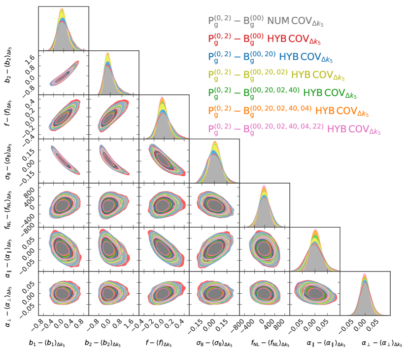
Refer to caption
Figure 10: 1- and 2-D marginalised parameters posterior distributions for different combinations of the bispectrum multipoles, Δk5Δsubscript𝑘5\Delta k_{5} case. Here we use the analytical model for a fiducial cosmology as data vector measurement. The gray (NUM COV) and red (HYB COV) contours are obtained using the same statistics (up to the bispectrum monopole) and covariance matrices as in Figure 5. The blue contours are obtained by adding to the data vector the quadrupole term relative to the angle between to the normal to the surface of the triangle and the line of sight ( [Pg(0,2);Bg(00,20)]superscriptsubscriptPg02superscriptsubscriptBg0020\mathrm{\left[\mathrm{P}_{\mathrm{g}}^{(0,2)};\mathrm{B}_{\mathrm{g}}^{(00,20)}\right]}). The yellow contours are obtained by including also the quadrupole term relative to the angle describing the rotation of the triangle around the normal to its surface ( [Pg(0,2);Bg(00,20,02)]superscriptsubscriptPg02superscriptsubscriptBg002002\mathrm{\left[\mathrm{P}_{\mathrm{g}}^{(0,2)};\mathrm{B}_{\mathrm{g}}^{(00,20,02)}\right]}). In the same way the green and orange contours show the effect of adding the hexadecapoles terms of the two angles in the same order ([Pg(0,2);Bg(00,20,02,40)]superscriptsubscriptPg02superscriptsubscriptBg00200240\mathrm{\left[\mathrm{P}_{\mathrm{g}}^{(0,2)};\mathrm{B}_{\mathrm{g}}^{(00,20,02,40)}\right]} and [Pg(0,2);Bg(00,20,02,40,04)]superscriptsubscriptPg02superscriptsubscriptBg0020024004\mathrm{\left[\mathrm{P}_{\mathrm{g}}^{(0,2)};\mathrm{B}_{\mathrm{g}}^{(00,20,02,40,04)}\right]}), respectively. The addition of the last hexadecapole term (quadrupoles of the two angles used for the polynomial expansion) is shown in pink contours ([Pg(0,2);Bg(00,20,02,40,04,22)]superscriptsubscriptPg02superscriptsubscriptBg002002400422\mathrm{\left[\mathrm{P}_{\mathrm{g}}^{(0,2)};\mathrm{B}_{\mathrm{g}}^{(00,20,02,40,04,22)}\right]}). The main message that this figure conveys, together with Table 2, is that significant parameter constraints improvements are obtained up to the bispectrum hexadecapole level.

6.2 Improvement on parameter constraints

Because of the lack of measurements for the multipoles Bg(20)superscriptsubscript𝐵𝑔20B_{g}^{(20)}, Bg(02)superscriptsubscript𝐵𝑔02B_{g}^{(02)}, Bg(40)superscriptsubscript𝐵𝑔40B_{g}^{(40)} , Bg(04)superscriptsubscript𝐵𝑔04B_{g}^{(04)} and Bg(22)superscriptsubscript𝐵𝑔22B_{g}^{(22)} we use an analytical data vector computed for our fiducial cosmology. Figure 10 shows the 1 and 2D posterior distributions of the cosmological parameters for data vectors of different lengths, starting from the basic power spectrum monopole and quadruple and bispectrum monopole, higher bispectrum multiplies are gradually added. Since in the previous tests comparing analytic/hybrid and numerical covariance matrix the data vector was taken from the mocks, in Figure 10 (gray and red) we repeat the comparison of sec. 5.2 using analytic the data vector. Also in the case of the analytical template for the data vector, the results obtained with numerical and hybrid covariance matrices are in very good agreement.

The 1-2D marginalised contours shown in Figure 10 confirm what deduced from the signal to noise study (Figure 9): saturation is achieved at the bispectrum hexadecapole level.

We observe a shrinkage of the 1- and 2-D marginalised posterior distributions as galaxy bispectrum higher multipoles are employed with respect to the monopole term alone. This aspect, together with the saturation, is quantitatively described in Table 2. This analysis suggests that including all the terms up to the galaxy bispectrum hexadecapoles (together with the power spectrum monopole and quadrupole), results in improving the 1D 68%percent6868\% credible regions by a factor of 30%similar-toabsentpercent30\sim 30\% on average – equivalent to observing a volume in the sky 2similar-toabsent2\sim 2 times larger (V(ıȷ)1/σıȷ21/(0.7σ(00))2=2×V(00)proportional-tosubscript𝑉italic-ıitalic-ȷ1subscriptsuperscript𝜎2italic-ıitalic-ȷsimilar-to-or-equals1superscript0.7subscript𝜎0022subscript𝑉00V_{(\imath\jmath)}\propto 1/\sigma^{2}_{\imath\jmath}\simeq 1/(0.7\,\sigma_{(00)})^{2}=2\times V_{(00)}).

Recall that our analysis is very conservative in terms of scales, by setting kmax=0.09h/Mpcsubscript𝑘max0.09Mpck_{\mathrm{max}}=0.09\,h/\mathrm{Mpc} we restrict our investigation to the linear regime. Extension to the mildly non-linear regime may offer additional gains. The cumulative signal to noise shown in Figure 9 seems to hint that, as kmaxsubscript𝑘maxk_{\mathrm{max}} increases, the difference between the isotropic (monopole) and isotropic plus anistropic (monopole plus higher multipoles) bispectrum signal may also increase.

This trend will eventually stop, as Figure 7 of [88] seems to indicate around kmax0.20h/Mpcsimilar-to-or-equalssubscript𝑘max0.20Mpck_{\mathrm{max}}\simeq 0.20\,h/\mathrm{Mpc}, however it would leave a non negligible gap between the isotropic and anisotropic signal to noise ratios. Therefore as smaller and smaller scales are considered, the signal to noise difference would likely translate into a stronger impact of the anisotropic bispectrum signal in terms of parameter constraints improvements. Full investigation in this direction is left for future work.

statistics ΔθPg(0,2);Bg(00)num.cov.ΔθPg(0,2);Bg(ı,ȷ)hyb.cov.ΔθPg(0,2);Bg(00)num.cov.[%]\dfrac{\Delta\theta^{\mathrm{num.\,cov.}}_{\mathrm{P_{g}^{(0,2)};B_{g}^{(00)}}}-\Delta\theta^{\mathrm{hyb.\,cov.}}_{\mathrm{P_{g}^{(0,2)};B_{g}^{(\imath,\jmath)}}}}{\Delta\theta^{\mathrm{num.\,cov.}}_{\mathrm{P_{g}^{(0,2)};B_{g}^{(00)}}}}\;\left[\%\right]
Pg(0,2)+limit-fromsuperscriptsubscriptPg02\mathrm{P}_{\mathrm{g}}^{(0,2)}\;+ b1subscript𝑏1b_{1} b2subscript𝑏2b_{2} f𝑓f σ8subscript𝜎8\sigma_{8} fNLsubscript𝑓NLf_{\mathrm{NL}} αsubscript𝛼parallel-to\alpha_{\parallel} αsubscript𝛼perpendicular-to\alpha_{\perp} average
Bg(00)superscriptsubscriptBg00\mathrm{\mathrm{B}_{\mathrm{g}}^{(00)}} 2.6 3.0 -5.0 3.1 0.4 -6.6 -0.7 -0.5
Bg(00,20)superscriptsubscriptBg0020\mathrm{\mathrm{B}_{\mathrm{g}}^{(00,20)}} 13.0 17.2 10.7 11.8 7.2 2.7 5.0 9.7
Bg(00,20,02)superscriptsubscriptBg002002\mathrm{\mathrm{B}_{\mathrm{g}}^{(00,20,02)}} 27.8 31.2 25.7 27.1 16.8 14.8 8.5 21.7
Bg(00,20,02,40)superscriptsubscriptBg00200240\mathrm{\mathrm{B}_{\mathrm{g}}^{(00,20,02,40)}} 26.9 30.8 28.0 25.2 17.0 19.3 11.4 22.7
Bg(00,20,02,40,04)superscriptsubscriptBg0020024004\mathrm{\mathrm{B}_{\mathrm{g}}^{(00,20,02,40,04)}} 31.0 34.1 36.5 30.1 25.3 31.0 18.2 29.5
Bg(00,20,02,40,04,22)superscriptsubscriptBg002002400422\mathrm{\mathrm{B}_{\mathrm{g}}^{(00,20,02,40,04,22)}} 29.9 33.6 36.6 28.4 28.5 32.1 21.2 30.0
Table 2: Relative improvements on the 1D 68%percent6868\% confidence intervals for the model parameters given by employing the quadrupole and hexadecapole terms of the galaxy bispectrum. In accordance with what observed for the cumulative signal to noise ratio and the 1-2D marginalised posterior distributions in Figures 9 and 10 respectively, we see that the saturation in terms of information is reached with the addition of the third bispectrum hexadecapole term (the largest constraints improvements have been highlighted using the bold font). As an additional check on the analytical data vector, the first row shows that there is a negligible difference between the constraints obtained using the analytical and numerical covariance matrix for the same data vector.
Refer to caption
Figure 11: Primordial non-Gaussianity signal in the bispectrum multipoles for fNL=5subscript𝑓NL5f_{\mathrm{NL}}=5. As indicated in the legend each line color/linestyle, corresponds to a different bispectrum multipole. The top panel shows the ratio between the primordial (Bg,1,1,1(ij)subscriptsuperscript𝐵𝑖𝑗g111B^{(ij)}_{\mathrm{g},1,1,1}) and the gravitational parts (Bg,1,1,2(ij)subscriptsuperscript𝐵𝑖𝑗g112B^{(ij)}_{\mathrm{g},1,1,2}). In the second panel from the top we show the ratio between each multipole’s primordial component and the variance given by the calibrated hybrid covariance matrix is displayed. This can be interpreted as a signal-to-noise ratio. In the third row, the cumulative signal to noise ratio of the primordial non-Gaussian bispectrum component is reported. Finally in the bottom panel the full bispectrum signal (primordial plus gravitational) for each multipole is plotted, always as a function of the triangle configurations. Once more the shaded regions correspond to the square root of the analytical covariance matrices diagonal elements.

6.3 Local Primordial non-Gaussianity

The bispectrum has been widely studied in the literature [93, 62, 83, 57, 82] as a powerful tool to constrain potential deviations from Gaussianity of the primordial gravitational potential [8]. By reducing the degeneracies between cosmological parameters, the galaxy bispectrum higher multipoles can play an important role in obtaining late-times constraints on the primordial non-Gaussianity amplitude parameter fNLsubscript𝑓NLf_{\mathrm{NL}} [10] competitive with the early times ones produced by cosmic microwave background (CMB) experiment such as Planck [2]. Moreover constraining fNLsubscript𝑓NLf_{\mathrm{NL}} using the bispectrum multipoles does not rely on extremely large scales and on highly biased tracers as the current state-of-the-art analysis of the power spectrum scale dependent bias [25].

In our estimate of the signature of primordial non-Gaussianity in the anisotropic bispectrum we do not include the modelling of the terms associated with the scale dependent bias induced by a local fNLsubscript𝑓NLf_{\mathrm{NL}} [30, 65] and arising from the multivariate bias expansion [41, 6, 90] applied to the bispectrum. This effect is particularly strong at very large scales and an analysis aimed at deriving constraints on the local non-Gaussianity amplitude parameter fNLsubscript𝑓NLf_{\mathrm{NL}} using the bispectrum should implement the modelling developed in [91, 60] which also includes the multivariate biasing expansion in redshift-space. Our analysis can be interpreted as a conservative estimate using only the primordial signal appearing from a non vanishing initial bispectrum, underestimating the actual signature given by fNL0subscript𝑓NL0f_{\mathrm{NL}}\neq 0. This would be larger and likely less correlated with the other cosmological parameters, especially on large scales, if we would include the non-local bias effect. This is possibly one of the reasons why we obtain larger confidence intervals for fNLsubscript𝑓NLf_{\mathrm{NL}} than the forecasts made through a Fisher information analysis in [91].

In particular redshift space distortions add an additional difference in the standard perturbation theory kernels dependence between the gravitational collapse (Bg,112(ıȷ)Z1sZ1sZ2sproportional-tosubscriptsuperscriptBitalic-ıitalic-ȷg112subscriptsuperscriptZs1subscriptsuperscriptZs1subscriptsuperscriptZs2\mathrm{B}^{(\imath\jmath)}_{\mathrm{g},112}\propto\mathrm{Z^{\mathrm{s}}_{1}}\mathrm{Z^{\mathrm{s}}_{1}}\mathrm{Z^{\mathrm{s}}_{2}}) and primordial (Bg,111(ıȷ)Z1sZ1sZ1sproportional-tosubscriptsuperscriptBitalic-ıitalic-ȷg111subscriptsuperscriptZs1subscriptsuperscriptZs1subscriptsuperscriptZs1\mathrm{B}^{(\imath\jmath)}_{\mathrm{g},111}\propto\mathrm{Z^{\mathrm{s}}_{1}}\mathrm{Z^{\mathrm{s}}_{1}}\mathrm{Z^{\mathrm{s}}_{1}}) components of the bispectrum which becomes more explicit when the anisotropic signal is studied.

In Figure 11 we show the local primordial non-Gaussianity contributions to the bispectrum [20] for the different multipoles, setting fNL=5subscript𝑓NL5f_{\mathrm{NL}}=5. These terms have been computed using the expression reported in the Appendix of [47]. The first row shows, for the different multipoles, the ratio between the primordial signal555It is interesting to notice that the multipoles that appear to be more sensitive to (richer in signal for) local primordial non-Gaussianity, are the ones relative to the angle describing the triangle rotation around the normal to the surface. An hint for a potential explanation to this effect could be searched in the angle conversion Equation A.2. The cosine ν𝜈\nu of the angle describing the rotation of the triangle around the normal to the surface depends explicitly on cosαabsubscript𝛼𝑎𝑏\cos\alpha_{ab}. This is the cosine of the internal angle of the triangle projection on the plane perpendicular to the line of sight. Therefore ν𝜈\nu explicitly depends on how much squeezed is the triangle, which is a factor known to influence the sensitivity to primordial non-Gaussianity [35, 6, 21, 64]. Bg,111(ıȷ)subscriptsuperscriptBıȷg111\mathrm{B^{(\imath\jmath)}_{g,111}} and the gravitational collapse part of the bispectrum Bg,112(ıȷ)subscriptsuperscriptBıȷg112\mathrm{B^{(\imath\jmath)}_{g,112}}. In the second panel from the top, the ratio is between Bg,111(ıȷ)subscriptsuperscriptBıȷg111\mathrm{B^{(\imath\jmath)}_{g,111}} and the variance computed using the analytical covariance matrix model used in the paper’s analysis. On the third row, the comulative signal-to-noise ratio is shown as a function of the number of triangle configurations included in the data vector. Finally in the bottom panel it is possible to see the total signal (primordial plus gravitational) for the different multipoles as a function of the triangle configurations considered.

7 Conclusions

At the power spectrum level, it is well known that the anisotropic modulation of the signal with respect to the line-of-sight induced by redshift space distortions carries valuable cosmological information. This anisotropy is usually expressed in multipole moments: the monopole –being the averaged signal in all directions around the line of sight– and the quadruple. The bispectrum has been proved useful for breaking degeneracies among parameters and detecting specific physical signatures (e.g., the so-called GR effects or neutrino masses). To date, only the bispectrum monopole has been used to constrain cosmological parameters from galaxy spectroscopic surveys. Measuring higher-order multipoles of the redshift-space galaxy bispectrum is indeed challenging and computationally expensive [76, 52, 89]. In this paper we have addressed the question: given these challenges, is it worth it? We consider that the answer is "yes", if adding the bispectrum anisotropic signal to the standard power spectrum Pg()superscriptsubscriptPg\mathrm{P}_{\mathrm{g}}^{(\ell)} (isotropic + anisotropic) and bispectrum Bg(00)superscriptsubscriptBg00\mathrm{B}_{\mathrm{g}}^{(00)} (isotropic) data vector, produces tighter 1- and 2-D marginalised posterior distributions for the parameters usually constrained by galaxy-clustering analyses.

To do so, we developed an analytical model for the full covariance matrix including power spectrum monopole and quadruple and bispectrum monopole and higher-orders multipoles up to the hexadecapole, for a conservative range of scales (kmax=0.09h/Mpcsubscript𝑘max0.09Mpck_{\mathrm{max}}=0.09\,h/\mathrm{Mpc}). We concentrated on the set of cosmological parameters (b1,b2,f,σ8,fNL,α,α)subscript𝑏1subscript𝑏2𝑓subscript𝜎8subscript𝑓NLsubscript𝛼perpendicular-tosubscript𝛼parallel-to(b_{1},b_{2},f,\sigma_{8},f_{\mathrm{NL}},\alpha_{\perp},\alpha_{\parallel}).

We first calibrate the analytical covariance matrix on the one estimated numerically from a suite of 1400 mock survey catalogs. The calibration is done on the sub-matrix corresponding to the reduced data vector [Pg(0,2);Bg(00)]superscriptsubscriptPg02superscriptsubscriptBg00\mathrm{\left[\mathrm{P}_{\mathrm{g}}^{(0,2)};\mathrm{B}_{\mathrm{g}}^{(00)}\right]}. We have shown that the parameter’s 1- and 2-D marginalised posteriors distributions obtained with our analytical covariance and the numerical one are very similar and basically indistinguishable for practical applications of reporting error-bars on parameters values (Figures 5, 6, 7).

Forecasts of the improvements in terms of parameter constraints induced by adding to the data vector the galaxy bispectrum anisotropic signal were presented in Section 6. These have been obtained by running standard MCMC samplings together with using the analytical covariance matrix to evaluate the likelihood. For a BOSS-like survey, we found on average 22%similar-toabsentpercent22\sim 22\% tighter 1D 68%percent6868\% credible regions by just considering the two bispectrum quadrupoles in addition to the monopole (Figure 10 and Table 2).

Including the last galaxy bispectrum hexadecapole term Bg(22)superscriptsubscriptBg22\mathrm{B_{g}}^{(22)} only returns a further smaller improvement, suggesting that the constraining power of the bispectrum saturates at this level when expanded in terms of Legendre polynomials. This hypothesis is supported by the behaviour of the signal to noise ratio in Figure 9 and 1-2D marginalised posterior distributions (again Figure 10 and Table 2), where adding the third hexadecapole term, Bg(22)superscriptsubscriptBg22\mathrm{B_{g}^{(22)}}, does not provide any significant information gain. Improving by 30%similar-toabsentpercent30\sim 30\% on average the parameter constraints by employing the bispectrum anisotropic signal approximately corresponds to observing a survey volume two times larger for a BOSS-like survey.

We stress that these results are conservative since we restrict our analysis to linear scales kmax=0.09hsubscript𝑘max0.09k_{\mathrm{max}}=0.09\,h/Mpc. Cumulative signal to noise studies in the literature indicate that the benefits of both employing the anisotropic bispectrum [88] and adding the bispectrum to the power spectrum analyses [84, 22, 96], increase for larger kmaxsubscript𝑘maxk_{\mathrm{max}}.

In Appendix D we report the key Figures displaying the results obtained when the same analysis done in the main body of the paper is also performed on the bispectrum data vector obtained for a larger k𝑘k-bin width (Δk6Δsubscript𝑘6\Delta k_{6}), hence with less triangle configurations. Even if the overall improvement on the parameters constraints appears to be larger, information gain saturation is again reached at the bispectrum hexadecapole level. Moreover, comparing the 1- and 2-D marginalised posterior distributions for the two k𝑘k-bin width cases, Figure 10 for Δk5Δsubscript𝑘5\Delta k_{5} and Figure 15 for Δk6Δsubscript𝑘6\Delta k_{6}, we appreciate that the contours for the full data vector including all the multipoles up to the hexadecapole level are qualitatively very similar.

We therefore conclude that the (significant) effort necessary to include the bispectrum quadruple in clustering analysis of galaxy redshift surveys is very likely to pay off. We envision that this extra information could be used not only to reduce parameter errors; these additional statistics can provide a useful consistency checks of the modelling itself but possibly also of the model.

Appendix A Covariance matrix terms derivation

In this Appendix are reported the full derivations of the covariance terms used in this work. We build on and improve what already presented in a previous paper [48]. In particular we are interested in computing the covariance expressions for both power spectrum and bispectrum expansion in terms of Legendre polynomials encoding the relation between the signal and the k𝑘k-vectors orientation with respect to the line of sight.

A.1 Power spectrum multipoles auto-covariance

In order to compute the covariance of the power spectrum multipoles it is necessary to evaluate the four-point correlator in Fourier space:

δg(𝐤1)δg(𝐤1)δg(𝐤2)δg(𝐤2)delimited-⟨⟩subscript𝛿gsubscript𝐤1subscript𝛿gsubscript𝐤1subscript𝛿gsubscript𝐤2subscript𝛿gsubscript𝐤2\displaystyle\langle\delta_{\mathrm{g}}(\mathbf{k}_{1})\delta_{\mathrm{g}}(-\mathbf{k}_{1})\delta_{\mathrm{g}}(\mathbf{k}_{2})\delta_{\mathrm{g}}(-\mathbf{k}_{2})\rangle =δg(𝐤1)δg(𝐤2)cδg(𝐤2)δg(𝐤1)c+ 1perm.absentsubscriptdelimited-⟨⟩subscript𝛿gsubscript𝐤1subscript𝛿gsubscript𝐤2csubscriptdelimited-⟨⟩subscript𝛿gsubscript𝐤2subscript𝛿gsubscript𝐤1c1perm\displaystyle=\langle\delta_{\mathrm{g}}(\mathbf{k}_{1})\delta_{\mathrm{g}}(-\mathbf{k}_{2})\rangle_{\mathrm{c}}\langle\delta_{\mathrm{g}}(\mathbf{k}_{2})\delta_{\mathrm{g}}(-\mathbf{k}_{1})\rangle_{\mathrm{c}}+\,1\,\mathrm{perm.}
+δg(𝐤1)δg(𝐤2)δg(𝐤1)δg(𝐤2)c,subscriptdelimited-⟨⟩subscript𝛿gsubscript𝐤1subscript𝛿gsubscript𝐤2subscript𝛿gsubscript𝐤1subscript𝛿gsubscript𝐤2c\displaystyle+\langle\delta_{\mathrm{g}}(\mathbf{k}_{1})\delta_{\mathrm{g}}(\mathbf{k}_{2})\delta_{\mathrm{g}}(-\mathbf{k}_{1})\delta_{\mathrm{g}}(-\mathbf{k}_{2})\rangle_{\mathrm{c}}, (A.1)

where the term in the second line is proportional to the trispectrum for parallelogram configurations. Since we limit our analysis to linear scales, we only use the first Gaussian term, which dominates over the non-Gaussian one. For a recent work regarding the power spectrum covariance matrix see [95]. It is possible to compute the Gaussian term of the covariance for the power spectrum monopole and quadrupole as follows:

CGPg()Pg()(k1;k2)=(2+1)2(2π)6Np(k1)Np(k2)V𝐪1V𝐪2V𝐩1V𝐩2d3𝐪1d3𝐪2d3𝐩1d3𝐩2superscriptsubscriptCGsubscriptsuperscriptPgsubscriptsuperscriptPgsubscript𝑘1subscript𝑘2superscript212superscript2𝜋6subscript𝑁psubscript𝑘1subscript𝑁psubscript𝑘2subscriptsubscript𝑉subscript𝐪1subscriptsubscript𝑉subscript𝐪2subscriptsubscript𝑉subscript𝐩1subscriptsubscript𝑉subscript𝐩2superscript𝑑3subscript𝐪1superscript𝑑3subscript𝐪2superscript𝑑3subscript𝐩1superscript𝑑3subscript𝐩2\displaystyle\mathrm{C}_{\mathrm{G}}^{\mathrm{P}^{(\ell)}_{\mathrm{g}}\mathrm{P}^{(\ell)}_{\mathrm{g}}}\left(k_{1};k_{2}\right)=\left(2\ell+1\right)^{2}\dfrac{(2\pi)^{-6}}{N_{\mathrm{p}}\left(k_{1}\right)N_{\mathrm{p}}\left(k_{2}\right)}\int_{V_{\mathbf{q}_{1}}}\int_{V_{\mathbf{q}_{2}}}\int_{V_{\mathbf{p}_{1}}}\int_{V_{\mathbf{p}_{2}}}d^{3}\mathbf{q}_{1}d^{3}\mathbf{q}_{2}d^{3}\mathbf{p}_{1}d^{3}\mathbf{p}_{2}
×(μ1)(μ2)δD(𝐪1+𝐩1)δD(𝐪2+𝐩2)2(2π)6δD(𝐪1+𝐪2)δD(𝐩1+𝐩2)Pgs(𝐪1)Pgs(𝐩2)absentsubscriptsubscript𝜇1subscriptsubscript𝜇2subscript𝛿𝐷subscript𝐪1subscript𝐩1subscript𝛿𝐷subscript𝐪2subscript𝐩22superscript2𝜋6subscript𝛿𝐷subscript𝐪1subscript𝐪2subscript𝛿𝐷subscript𝐩1subscript𝐩2superscriptsubscriptPgssubscript𝐪1superscriptsubscriptPgssubscript𝐩2\displaystyle\times\mathcal{L}_{\ell}\left(\mu_{1}\right)\mathcal{L}_{\ell}\left(\mu_{2}\right)\delta_{D}\left(\mathbf{q}_{1}+\mathbf{p}_{1}\right)\delta_{D}\left(\mathbf{q}_{2}+\mathbf{p}_{2}\right)2(2\pi)^{6}\delta_{D}\left(\mathbf{q}_{1}+\mathbf{q}_{2}\right)\delta_{D}\left(\mathbf{p}_{1}+\mathbf{p}_{2}\right)\mathrm{P}_{\mathrm{g}}^{\mathrm{s}}\left(\mathbf{q}_{1}\right)\mathrm{P}_{\mathrm{g}}^{\mathrm{s}}\left(\mathbf{p}_{2}\right)
=(2+1)22Np(k1)Np(k2)V𝐪1V𝐪2d3𝐪1d3𝐪2(μ1)(μ2)δD(𝐪1+𝐪2)2Pgs(𝐪1)Pgs(𝐪2)absentsuperscript2122subscript𝑁psubscript𝑘1subscript𝑁psubscript𝑘2subscriptsubscript𝑉subscript𝐪1subscriptsubscript𝑉subscript𝐪2superscript𝑑3subscript𝐪1superscript𝑑3subscript𝐪2subscriptsubscript𝜇1subscriptsubscript𝜇2subscript𝛿𝐷superscriptsubscript𝐪1subscript𝐪22superscriptsubscriptPgssubscript𝐪1superscriptsubscriptPgssubscript𝐪2\displaystyle=\left(2\ell+1\right)^{2}\dfrac{2}{N_{\mathrm{p}}\left(k_{1}\right)N_{\mathrm{p}}\left(k_{2}\right)}\int_{V_{\mathbf{q}_{1}}}\int_{V_{\mathbf{q}_{2}}}d^{3}\mathbf{q}_{1}d^{3}\mathbf{q}_{2}\mathcal{L}_{\ell}\left(\mu_{1}\right)\mathcal{L}_{\ell}\left(\mu_{2}\right)\delta_{D}\left(\mathbf{q}_{1}+\mathbf{q}_{2}\right)^{2}\mathrm{P}_{\mathrm{g}}^{\mathrm{s}}\left(\mathbf{q}_{1}\right)\mathrm{P}_{\mathrm{g}}^{\mathrm{s}}\left(\mathbf{q}_{2}\right)
=(2+1)22Np(k1)Vp(k2)V𝐪1V𝐪2d3𝐪1d3𝐪2(μ1)(μ2)δD(𝐪1+𝐪2)Pgs(𝐪1)Pgs(𝐪2)absentsuperscript2122subscript𝑁psubscript𝑘1subscript𝑉psubscript𝑘2subscriptsubscript𝑉subscript𝐪1subscriptsubscript𝑉subscript𝐪2superscript𝑑3subscript𝐪1superscript𝑑3subscript𝐪2subscriptsubscript𝜇1subscriptsubscript𝜇2subscript𝛿𝐷subscript𝐪1subscript𝐪2superscriptsubscriptPgssubscript𝐪1superscriptsubscriptPgssubscript𝐪2\displaystyle=\left(2\ell+1\right)^{2}\dfrac{2}{N_{\mathrm{p}}\left(k_{1}\right)V_{\mathrm{p}}\left(k_{2}\right)}\int_{V_{\mathbf{q}_{1}}}\int_{V_{\mathbf{q}_{2}}}d^{3}\mathbf{q}_{1}d^{3}\mathbf{q}_{2}\mathcal{L}_{\ell}\left(\mu_{1}\right)\mathcal{L}_{\ell}\left(\mu_{2}\right)\delta_{D}\left(\mathbf{q}_{1}+\mathbf{q}_{2}\right)\mathrm{P}_{\mathrm{g}}^{\mathrm{s}}\left(\mathbf{q}_{1}\right)\mathrm{P}_{\mathrm{g}}^{\mathrm{s}}\left(\mathbf{q}_{2}\right)
(2+1)22kf3Vp(k1)1211𝑑μ1(μ1)2Pg(k1,μ1)2absentsuperscript2122superscriptsubscript𝑘𝑓3subscript𝑉psubscript𝑘112subscriptsuperscript11differential-dsubscript𝜇1subscriptsuperscriptsubscript𝜇12subscriptPgsuperscriptsubscript𝑘1subscript𝜇12\displaystyle\approx\left(2\ell+1\right)^{2}\dfrac{2k_{f}^{3}}{V_{\mathrm{p}}\left(k_{1}\right)}\quad\dfrac{1}{2}\int^{1}_{-1}d\mu_{1}\mathcal{L}_{\ell}\left(\mu_{1}\right)^{2}\mathrm{P}_{\mathrm{g}}\left(k_{1},\mu_{1}\right)^{2}
=(2+1)22kf3δ12K4πk12Δk1211𝑑μ1(μ1)2Pg(k1,μ1)2,absentsuperscript2122superscriptsubscript𝑘𝑓3subscriptsuperscript𝛿K124𝜋superscriptsubscript𝑘12Δ𝑘12subscriptsuperscript11differential-dsubscript𝜇1subscriptsuperscriptsubscript𝜇12subscriptPgsuperscriptsubscript𝑘1subscript𝜇12\displaystyle=\left(2\ell+1\right)^{2}\dfrac{2k_{f}^{3}\delta^{\mathrm{K}}_{12}}{4\pi k_{1}^{2}\Delta k}\quad\dfrac{1}{2}\int^{1}_{-1}d\mu_{1}\mathcal{L}_{\ell}\left(\mu_{1}\right)^{2}\mathrm{P}_{\mathrm{g}}\left(k_{1},\mu_{1}\right)^{2}, (A.2)

where again we used the approximation made in [58] that δD2Vs(2π)3δD=kf3δDsuperscriptsubscript𝛿D2subscript𝑉ssuperscript2𝜋3subscript𝛿Dsuperscriptsubscript𝑘𝑓3subscript𝛿D\delta_{\mathrm{D}}^{2}\approx\dfrac{V_{\mathrm{s}}}{(2\pi)^{3}}\delta_{\mathrm{D}}=k_{f}^{-3}\delta_{\mathrm{D}}. Vssubscript𝑉sV_{\mathrm{s}} is the survey volume kfsubscript𝑘𝑓k_{f} the fundamental frequency. δ12Ksubscriptsuperscript𝛿K12\delta^{\mathrm{K}}_{12} is the Kronecker delta indicating that the vector 𝐪1subscript𝐪1\mathbf{q}_{1} and 𝐪2subscript𝐪2\mathbf{q}_{2} are identical (in the second step trivial δKsubscript𝛿K\delta_{\mathrm{K}} have been omitted in order to avoid making the notation heavier by adding also the wave-vector letter). The Fourier integration volume for the power spectrum is defined as Vp=4πΔkk2subscript𝑉p4𝜋Δ𝑘superscript𝑘2V_{\mathrm{p}}=4\pi\Delta kk^{2} and therefore the number of modes ("pairs") as Np=Vp/kf3subscript𝑁psubscript𝑉psuperscriptsubscript𝑘𝑓3N_{\mathrm{p}}=V_{\mathrm{p}}/k_{f}^{3}. {\cal L} denotes the Lagrange polynomials. In the last steps we made the approximation that the power spectrum monopole and quadrupoles do not significantly vary when integrated over the bin in Fourier space.

A.2 Bispectrum multipoles auto-covariance

We write these expression as functions of the multipoles of two angles defined in [52]. The first is the angle ω𝜔\omega between the normal to the surface of the triangle and the line of sight. The second is the angle ϕitalic-ϕ\phi between the first k-vector and one of the two axis defining the plane on which the triangle lies. We will then use the cosines for the multipoles μ=cosω𝜇𝜔\mu=\cos\omega and ν=cosϕ𝜈italic-ϕ\nu=\cos\phi. The multipoles indexes will be given then by μa(α)subscriptsuperscript𝛼subscript𝜇𝑎\mathcal{L}^{(\alpha)}_{\mu_{a}}, νa(β)subscriptsuperscript𝛽subscript𝜈𝑎\mathcal{L}^{(\beta)}_{\nu_{a}} for the first triangle and μb(κ)subscriptsuperscript𝜅subscript𝜇𝑏\mathcal{L}^{(\kappa)}_{\mu_{b}}, νb(λ)subscriptsuperscript𝜆subscript𝜈𝑏\mathcal{L}^{(\lambda)}_{\nu_{b}} for the second one. We introduce the short notation μν,ab(αβκλ)=μa(α)νa(β)μb(κ)νb(λ)subscriptsuperscript𝛼𝛽𝜅𝜆𝜇𝜈𝑎𝑏subscriptsuperscript𝛼subscript𝜇𝑎subscriptsuperscript𝛽subscript𝜈𝑎subscriptsuperscript𝜅subscript𝜇𝑏subscriptsuperscript𝜆subscript𝜈𝑏\mathcal{M}^{(\alpha\beta\kappa\lambda)}_{\mu\nu,ab}=\mathcal{L}^{(\alpha)}_{\mu_{a}}\mathcal{L}^{(\beta)}_{\nu_{a}}\mathcal{L}^{(\kappa)}_{\mu_{b}}\mathcal{L}^{(\lambda)}_{\nu_{b}}. In the same way we will write the compact pre-factor 𝒞κλαβ=(2α+1)(2β+1)(2κ+1)(2λ+1)subscriptsuperscript𝒞𝛼𝛽𝜅𝜆2𝛼12𝛽12𝜅12𝜆1\mathcal{C}^{\alpha\beta}_{\kappa\lambda}=(2\alpha+1)(2\beta+1)(2\kappa+1)(2\lambda+1).

Following the angles definition in [52], the conversion from the standard bispectrum coordinates (k1,k2,k3,μ1,μ2)subscript𝑘1subscript𝑘2subscript𝑘3subscript𝜇1subscript𝜇2(k_{1},k_{2},k_{3},\mu_{1},\mu_{2}) to the set used in this work (k1,k2,k3,μ,ν)subscript𝑘1subscript𝑘2subscript𝑘3𝜇𝜈(k_{1},k_{2},k_{3},\mu,\nu) is given by

μ=cosω𝜇𝜔\displaystyle\mu=\cos\omega =2(a2b2+a2c2+b2c2)a4b4c42(a2b2+a2c2+b2c2)a4b4c4=ΔΔabsent2superscriptsubscript𝑎perpendicular-to2superscriptsubscript𝑏perpendicular-to2superscriptsubscript𝑎perpendicular-to2superscriptsubscript𝑐perpendicular-to2superscriptsubscript𝑏perpendicular-to2superscriptsubscript𝑐perpendicular-to2superscriptsubscript𝑎perpendicular-to4superscriptsubscript𝑏perpendicular-to4superscriptsubscript𝑐perpendicular-to42superscript𝑎2superscript𝑏2superscript𝑎2superscript𝑐2superscript𝑏2superscript𝑐2superscript𝑎4superscript𝑏4superscript𝑐4subscriptΔperpendicular-toΔ\displaystyle=\sqrt{\dfrac{2\left(a_{\perp}^{2}b_{\perp}^{2}+a_{\perp}^{2}c_{\perp}^{2}+b_{\perp}^{2}c_{\perp}^{2}\right)-a_{\perp}^{4}-b_{\perp}^{4}-c_{\perp}^{4}}{2\left(a^{2}b^{2}+a^{2}c^{2}+b^{2}c^{2}\right)-a^{4}-b^{4}-c^{4}}}=\sqrt{\dfrac{\Delta_{\perp}}{\Delta}}
ν=cosϕ𝜈italic-ϕ\displaystyle\nu=\cos\phi =(1μa2)μb+cosαabμa1μa21μb21μ2,absent1superscriptsubscript𝜇𝑎2subscript𝜇𝑏subscript𝛼𝑎𝑏subscript𝜇𝑎1superscriptsubscript𝜇𝑎21superscriptsubscript𝜇𝑏21superscript𝜇2\displaystyle=\dfrac{\left(1-\mu_{a}^{2}\right)\mu_{b}+\cos\alpha_{ab}\mu_{a}\sqrt{1-\mu_{a}^{2}}\sqrt{1-\mu_{b}^{2}}}{\sqrt{1-\mu^{2}}}\,, (A.3)

where for notation simplicity we used (a,b,c)𝑎𝑏𝑐(a,b,c) instead of (k1,k2,k3)subscript𝑘1subscript𝑘2subscript𝑘3(k_{1},k_{2},k_{3}). The ’perpendicular-to\perp’ indicates the 2D vector obtained by projecting the 3D k𝑘k-vector onto to the plane perpendicular to the line of sight. αabsubscript𝛼𝑎𝑏\alpha_{ab} is the internal angle between the sides asubscript𝑎perpendicular-toa_{\perp} and bsubscript𝑏perpendicular-tob_{\perp} of the abcsubscript𝑎perpendicular-tosubscript𝑏perpendicular-tosubscript𝑐perpendicular-toa_{\perp}b_{\perp}c_{\perp} triangle. When |μ|=1𝜇1|\mu|=1 the triangle normal to the surface is either parallel or anti-parallel to the line of sight. Therefore the anisotropic bispectrum signal is the same for all the potential values of ν𝜈\nu since the triangle plane coincides with the one perpendicular to the line of sight.

In order to compute the covariance between two galaxy bispectrum multipoles, the six-points correlator in Fourier space given by the respective galaxy density variables needs to be evaluated [85]:

\displaystyle\langle δg(𝐤1)δg(𝐤2)δg(𝐤3)δg(𝐤4)δg(𝐤5)δg(𝐤6)\displaystyle\delta_{\mathrm{g}}(\mathbf{k}_{1})\delta_{\mathrm{g}}(\mathbf{k}_{2})\delta_{\mathrm{g}}(\mathbf{k}_{3})\delta_{\mathrm{g}}(\mathbf{k}_{4})\delta_{\mathrm{g}}(\mathbf{k}_{5})\delta_{\mathrm{g}}(\mathbf{k}_{6})\rangle
=δg(𝐤1)δg(𝐤4)cδg(𝐤2)δg(𝐤5)cδg(𝐤3)δg(𝐤6)c+ 8perms.absentsubscriptdelimited-⟨⟩subscript𝛿gsubscript𝐤1subscript𝛿gsubscript𝐤4csubscriptdelimited-⟨⟩subscript𝛿gsubscript𝐤2subscript𝛿gsubscript𝐤5csubscriptdelimited-⟨⟩subscript𝛿gsubscript𝐤3subscript𝛿gsubscript𝐤6c8perms\displaystyle=\langle\delta_{\mathrm{g}}(\mathbf{k}_{1})\delta_{\mathrm{g}}(\mathbf{k}_{4})\rangle_{\mathrm{c}}\langle\delta_{\mathrm{g}}(\mathbf{k}_{2})\delta_{\mathrm{g}}(\mathbf{k}_{5})\rangle_{\mathrm{c}}\langle\delta_{\mathrm{g}}(\mathbf{k}_{3})\delta_{\mathrm{g}}(\mathbf{k}_{6})\rangle_{\mathrm{c}}+\,8\,\mathrm{perms.}
+δg(𝐤1)δg(𝐤2)δg(𝐤4)cδg(𝐤3)δg(𝐤5)δg(𝐤6)c+ 8perms.subscriptdelimited-⟨⟩subscript𝛿gsubscript𝐤1subscript𝛿gsubscript𝐤2subscript𝛿gsubscript𝐤4csubscriptdelimited-⟨⟩subscript𝛿gsubscript𝐤3subscript𝛿gsubscript𝐤5subscript𝛿gsubscript𝐤6c8perms\displaystyle+\langle\delta_{\mathrm{g}}(\mathbf{k}_{1})\delta_{\mathrm{g}}(\mathbf{k}_{2})\delta_{\mathrm{g}}(\mathbf{k}_{4})\rangle_{\mathrm{c}}\langle\delta_{\mathrm{g}}(\mathbf{k}_{3})\delta_{\mathrm{g}}(\mathbf{k}_{5})\delta_{\mathrm{g}}(\mathbf{k}_{6})\rangle_{\mathrm{c}}+\,8\,\mathrm{perms.}
+δg(𝐤1)δg(𝐤2)δg(𝐤5)δg(𝐤6)cδg(𝐤3)δg(𝐤4)c+ 8perms.subscriptdelimited-⟨⟩subscript𝛿gsubscript𝐤1subscript𝛿gsubscript𝐤2subscript𝛿gsubscript𝐤5subscript𝛿gsubscript𝐤6csubscriptdelimited-⟨⟩subscript𝛿gsubscript𝐤3subscript𝛿gsubscript𝐤4c8perms\displaystyle+\langle\delta_{\mathrm{g}}(\mathbf{k}_{1})\delta_{\mathrm{g}}(\mathbf{k}_{2})\delta_{\mathrm{g}}(\mathbf{k}_{5})\delta_{\mathrm{g}}(\mathbf{k}_{6})\rangle_{\mathrm{c}}\langle\delta_{\mathrm{g}}(\mathbf{k}_{3})\delta_{\mathrm{g}}(\mathbf{k}_{4})\rangle_{\mathrm{c}}+\,8\,\mathrm{perms.}
+δg(𝐤1)δg(𝐤2)δg(𝐤3)δg(𝐤4)δg(𝐤5)δg(𝐤6)c.subscriptdelimited-⟨⟩subscript𝛿gsubscript𝐤1subscript𝛿gsubscript𝐤2subscript𝛿gsubscript𝐤3subscript𝛿gsubscript𝐤4subscript𝛿gsubscript𝐤5subscript𝛿gsubscript𝐤6c\displaystyle+\langle\delta_{\mathrm{g}}(\mathbf{k}_{1})\delta_{\mathrm{g}}(\mathbf{k}_{2})\delta_{\mathrm{g}}(\mathbf{k}_{3})\delta_{\mathrm{g}}(\mathbf{k}_{4})\delta_{\mathrm{g}}(\mathbf{k}_{5})\delta_{\mathrm{g}}(\mathbf{k}_{6})\rangle_{\mathrm{c}}. (A.4)

From the above expression the bispectrum covariance results composed by four terms. The first is the so called Gaussian term which being proportional to the cube of the power spectrum represents the lowest order in the perturbation expansion (δm6proportional-toabsentsuperscriptsubscript𝛿m6\propto\delta_{\mathrm{m}}^{6} where "m" indicates the matter density field). The second and third terms are the lowest order non-Gaussian contributions (δm8proportional-toabsentsuperscriptsubscript𝛿m8\propto\delta_{\mathrm{m}}^{8}), proportional to the product of two bispectra and power spectrum times trispectrum, respectively. The last is proportional to the pentaspectrum and since it is an higher order term than the previous ones (δm10proportional-toabsentsuperscriptsubscript𝛿m10\propto\delta_{\mathrm{m}}^{10}), it will not be computed explicitly.

Gaussian term:

Here we update and extend the work presented in [48]. Analogously to what done above, we now compute the diagonal term of the bispectrum multipoles covariance matrix:

CP3BgαβBgκλ(k1,k2,k3;k4,k5,k6)=superscriptsubscriptCproportional-toabsentsuperscriptP3subscriptsuperscriptB𝛼𝛽gsubscriptsuperscriptB𝜅𝜆gsubscript𝑘1subscript𝑘2subscript𝑘3subscript𝑘4subscript𝑘5subscript𝑘6absent\displaystyle\mathrm{C}_{\propto\mathrm{P}^{3}}^{\mathrm{B}^{\alpha\beta}_{\mathrm{g}}\mathrm{B}^{\kappa\lambda}_{\mathrm{g}}}\left(k_{1},k_{2},k_{3};k_{4},k_{5},k_{6}\right)=
=(2πkf)6𝒞κλαβN123tN456ti=16V𝐪id3𝐪iμν,ab(αβκλ)δD(𝐪1+𝐪2+𝐪3)δD(𝐪4+𝐪5+𝐪6)absentsuperscript2𝜋subscript𝑘𝑓6subscriptsuperscript𝒞𝛼𝛽𝜅𝜆subscriptsuperscript𝑁t123subscriptsuperscript𝑁t456subscriptsuperscriptproduct6𝑖1subscriptsubscript𝑉subscript𝐪𝑖superscript𝑑3subscript𝐪𝑖subscriptsuperscript𝛼𝛽𝜅𝜆𝜇𝜈𝑎𝑏subscript𝛿𝐷subscript𝐪1subscript𝐪2subscript𝐪3subscript𝛿𝐷subscript𝐪4subscript𝐪5subscript𝐪6\displaystyle=\dfrac{(2\pi k_{f})^{-6}\mathcal{C}^{\alpha\beta}_{\kappa\lambda}}{N^{\mathrm{t}}_{123}N^{\mathrm{t}}_{456}}\prod^{6}_{i=1}\int_{V_{\mathbf{q}_{i}}}d^{3}\mathbf{q}_{i}\mathcal{M}^{(\alpha\beta\kappa\lambda)}_{\mu\nu,ab}\delta_{D}\left(\mathbf{q}_{1}+\mathbf{q}_{2}+\mathbf{q}_{3}\right)\delta_{D}\left(\mathbf{q}_{4}+\mathbf{q}_{5}+\mathbf{q}_{6}\right)
×(2π)9δD(𝐪1+𝐪4)δD(𝐪2+𝐪5)δD(𝐪3+𝐪6)Pgs(𝐪1)Pgs(𝐪2)Pgs(𝐪3)+5perm.absentsuperscript2𝜋9subscript𝛿𝐷subscript𝐪1subscript𝐪4subscript𝛿𝐷subscript𝐪2subscript𝐪5subscript𝛿𝐷subscript𝐪3subscript𝐪6superscriptsubscriptPgssubscript𝐪1superscriptsubscriptPgssubscript𝐪2superscriptsubscriptPgssubscript𝐪35perm\displaystyle\times(2\pi)^{9}\delta_{D}\left(\mathbf{q}_{1}+\mathbf{q}_{4}\right)\delta_{D}\left(\mathbf{q}_{2}+\mathbf{q}_{5}\right)\delta_{D}\left(\mathbf{q}_{3}+\mathbf{q}_{6}\right)\mathrm{P}_{\mathrm{g}}^{\mathrm{s}}\left(\mathbf{q}_{1}\right)\mathrm{P}_{\mathrm{g}}^{\mathrm{s}}\left(\mathbf{q}_{2}\right)\mathrm{P}_{\mathrm{g}}^{\mathrm{s}}\left(\mathbf{q}_{3}\right)\;+5\;\mathrm{perm.}
=D456123(2π)3kf6𝒞κλαβN123t,2i=13V𝐪id3𝐪iμν,aa(αβκλ)δD(𝐪1+𝐪2+𝐪3)2Pgs(𝐪1)Pgs(𝐪2)Pgs(𝐪3)absentsubscriptsuperscriptD123456superscript2𝜋3superscriptsubscript𝑘𝑓6subscriptsuperscript𝒞𝛼𝛽𝜅𝜆subscriptsuperscript𝑁t2123subscriptsuperscriptproduct3𝑖1subscriptsubscript𝑉subscript𝐪𝑖superscript𝑑3subscript𝐪𝑖subscriptsuperscript𝛼𝛽𝜅𝜆𝜇𝜈𝑎𝑎subscript𝛿𝐷superscriptsubscript𝐪1subscript𝐪2subscript𝐪32superscriptsubscriptPgssubscript𝐪1superscriptsubscriptPgssubscript𝐪2superscriptsubscriptPgssubscript𝐪3\displaystyle=\dfrac{\mathrm{D}^{123}_{456}(2\pi)^{3}k_{f}^{-6}\mathcal{C}^{\alpha\beta}_{\kappa\lambda}}{N^{\mathrm{t},2}_{123}}\prod^{3}_{i=1}\int_{V_{\mathbf{q}_{i}}}d^{3}\mathbf{q}_{i}\mathcal{M}^{(\alpha\beta\kappa\lambda)}_{\mu\nu,aa}\delta_{D}\left(\mathbf{q}_{1}+\mathbf{q}_{2}+\mathbf{q}_{3}\right)^{2}\mathrm{P}_{\mathrm{g}}^{\mathrm{s}}\left(\mathbf{q}_{1}\right)\mathrm{P}_{\mathrm{g}}^{\mathrm{s}}\left(\mathbf{q}_{2}\right)\mathrm{P}_{\mathrm{g}}^{\mathrm{s}}\left(\mathbf{q}_{3}\right)
=D456123(2π)3kf9𝒞κλαβN123t,2i=13V𝐪id3𝐪iμν,aa(αβκλ)δD(𝐪1+𝐪2+𝐪3)Pgs(𝐪1)Pgs(𝐪2)Pgs(𝐪3)absentsubscriptsuperscriptD123456superscript2𝜋3superscriptsubscript𝑘𝑓9subscriptsuperscript𝒞𝛼𝛽𝜅𝜆subscriptsuperscript𝑁t2123subscriptsuperscriptproduct3𝑖1subscriptsubscript𝑉subscript𝐪𝑖superscript𝑑3subscript𝐪𝑖subscriptsuperscript𝛼𝛽𝜅𝜆𝜇𝜈𝑎𝑎subscript𝛿𝐷subscript𝐪1subscript𝐪2subscript𝐪3superscriptsubscriptPgssubscript𝐪1superscriptsubscriptPgssubscript𝐪2superscriptsubscriptPgssubscript𝐪3\displaystyle=\dfrac{\mathrm{D}^{123}_{456}(2\pi)^{3}k_{f}^{-9}\mathcal{C}^{\alpha\beta}_{\kappa\lambda}}{N^{\mathrm{t},2}_{123}}\prod^{3}_{i=1}\int_{V_{\mathbf{q}_{i}}}d^{3}\mathbf{q}_{i}\mathcal{M}^{(\alpha\beta\kappa\lambda)}_{\mu\nu,aa}\delta_{D}\left(\mathbf{q}_{1}+\mathbf{q}_{2}+\mathbf{q}_{3}\right)\mathrm{P}_{\mathrm{g}}^{\mathrm{s}}\left(\mathbf{q}_{1}\right)\mathrm{P}_{\mathrm{g}}^{\mathrm{s}}\left(\mathbf{q}_{2}\right)\mathrm{P}_{\mathrm{g}}^{\mathrm{s}}\left(\mathbf{q}_{3}\right)
=D456123(2π)3kf3𝒞κλαβV123t,2i=13V𝐪id3𝐪iμν,aa(αβκλ)δD(𝐪1+𝐪2+𝐪3)Pgs(𝐪1)Pgs(𝐪2)Pgs(𝐪3)absentsubscriptsuperscriptD123456superscript2𝜋3superscriptsubscript𝑘𝑓3subscriptsuperscript𝒞𝛼𝛽𝜅𝜆subscriptsuperscript𝑉t2123subscriptsuperscriptproduct3𝑖1subscriptsubscript𝑉subscript𝐪𝑖superscript𝑑3subscript𝐪𝑖subscriptsuperscript𝛼𝛽𝜅𝜆𝜇𝜈𝑎𝑎subscript𝛿𝐷subscript𝐪1subscript𝐪2subscript𝐪3superscriptsubscriptPgssubscript𝐪1superscriptsubscriptPgssubscript𝐪2superscriptsubscriptPgssubscript𝐪3\displaystyle=\dfrac{\mathrm{D}^{123}_{456}(2\pi)^{3}k_{f}^{3}\mathcal{C}^{\alpha\beta}_{\kappa\lambda}}{V^{\mathrm{t},2}_{123}}\prod^{3}_{i=1}\int_{V_{\mathbf{q}_{i}}}d^{3}\mathbf{q}_{i}\mathcal{M}^{(\alpha\beta\kappa\lambda)}_{\mu\nu,aa}\delta_{D}\left(\mathbf{q}_{1}+\mathbf{q}_{2}+\mathbf{q}_{3}\right)\mathrm{P}_{\mathrm{g}}^{\mathrm{s}}\left(\mathbf{q}_{1}\right)\mathrm{P}_{\mathrm{g}}^{\mathrm{s}}\left(\mathbf{q}_{2}\right)\mathrm{P}_{\mathrm{g}}^{\mathrm{s}}\left(\mathbf{q}_{3}\right)
D456123(2π)3kf3𝒞κλαβV123t14π1+1𝑑μ102π𝑑ϕμν,aa(αβκλ)Pg(k1,μ1)Pg(k2,μ2)Pg(k3,μ3),absentsubscriptsuperscriptD123456superscript2𝜋3superscriptsubscript𝑘𝑓3subscriptsuperscript𝒞𝛼𝛽𝜅𝜆subscriptsuperscript𝑉t12314𝜋subscriptsuperscript11differential-dsubscript𝜇1subscriptsuperscript2𝜋0differential-ditalic-ϕsubscriptsuperscript𝛼𝛽𝜅𝜆𝜇𝜈𝑎𝑎subscriptPgsubscript𝑘1subscript𝜇1subscriptPgsubscript𝑘2subscript𝜇2subscriptPgsubscript𝑘3subscript𝜇3\displaystyle\approx\dfrac{\mathrm{D}^{123}_{456}(2\pi)^{3}k_{f}^{3}\mathcal{C}^{\alpha\beta}_{\kappa\lambda}}{V^{\mathrm{t}}_{123}}\dfrac{1}{4\pi}\int^{+1}_{-1}d\mu_{1}\int^{2\pi}_{0}d\phi\mathcal{M}^{(\alpha\beta\kappa\lambda)}_{\mu\nu,aa}\mathrm{P}_{\mathrm{g}}\left(k_{1},\mu_{1}\right)\mathrm{P}_{\mathrm{g}}\left(k_{2},\mu_{2}\right)\mathrm{P}_{\mathrm{g}}\left(k_{3},\mu_{3}\right), (A.5)

where D456123subscriptsuperscriptD123456\mathrm{D}^{123}_{456} stands for all the possible permutations and has values 6,2,16216,2,1 respectively for equilateral, isosceles and scalene triangles. V123t=8π2k1k2k3Δk1Δk2Δk3subscriptsuperscript𝑉t1238superscript𝜋2subscript𝑘1subscript𝑘2subscript𝑘3Δsubscript𝑘1Δsubscript𝑘2Δsubscript𝑘3V^{\mathrm{t}}_{123}=8\pi^{2}k_{1}k_{2}k_{3}\Delta k_{1}\Delta k_{2}\Delta k_{3} is the integration volume in Fourier space for the bispectrum. The number of modes is then defined as N123t=V123t/kf6subscriptsuperscript𝑁t123subscriptsuperscript𝑉t123superscriptsubscript𝑘𝑓6N^{\mathrm{t}}_{123}=V^{\mathrm{t}}_{123}/k_{f}^{6}. Again, we have assumed that the power spectrum monopole does not vary significantly inside the integration volume. The angle ϕitalic-ϕ\phi is defined such as μ2μ1cosψ121μ121cosψ122cosϕsubscript𝜇2subscript𝜇1subscript𝜓121superscriptsubscript𝜇121superscriptsubscript𝜓122italic-ϕ\mu_{2}\equiv\mu_{1}\cos\psi_{12}-\sqrt{1-\mu_{1}^{2}}\sqrt{1-\cos\psi_{12}^{2}}\cos\phi where cosψ12(𝐤1𝐤2/(k1k2)\cos\psi_{12}\equiv(\mathbf{k}_{1}\cdot\mathbf{k}_{2}/(k_{1}k_{2}). In order to be sure of the symmetry of the numerical result we integrate for each possible combination of k𝑘k-vectors (k1,k2)subscript𝑘1subscript𝑘2(k_{1},k_{2}), (k1,k3)subscript𝑘1subscript𝑘3(k_{1},k_{3}) and (k2,k3)subscript𝑘2subscript𝑘3(k_{2},k_{3}).

non-Gaussian terms:

the following term (Bispectrum cross covariance BBproportional-toabsent𝐵𝐵\propto BB) was also presented in [48] and allows one to better capture the correlation between different triangle bins. It is one of the two non-Gaussian terms that appear in the bispectrum self-covariance matrix up to order δm8proportional-toabsentsuperscriptsubscript𝛿m8\propto\delta_{\mathrm{m}}^{8}.

CBBBgαβBgκλ(k1,k2,k3;k4,k5,k6)=superscriptsubscriptCproportional-toabsentBBsubscriptsuperscriptB𝛼𝛽gsubscriptsuperscriptB𝜅𝜆gsubscript𝑘1subscript𝑘2subscript𝑘3subscript𝑘4subscript𝑘5subscript𝑘6absent\displaystyle\mathrm{C}_{\propto\mathrm{BB}}^{\mathrm{B}^{\alpha\beta}_{\mathrm{g}}\mathrm{B}^{\kappa\lambda}_{\mathrm{g}}}\left(k_{1},k_{2},k_{3};k_{4},k_{5},k_{6}\right)=
=(2πkf)6𝒞κλαβN123tN456ti=16V𝐪id3𝐪iμν,ab(αβκλ)δD(𝐪1+𝐪2+𝐪3)δD(𝐪4+𝐪5+𝐪6)absentsuperscript2𝜋subscript𝑘𝑓6subscriptsuperscript𝒞𝛼𝛽𝜅𝜆subscriptsuperscript𝑁t123subscriptsuperscript𝑁t456subscriptsuperscriptproduct6𝑖1subscriptsubscript𝑉subscript𝐪𝑖superscript𝑑3subscript𝐪𝑖subscriptsuperscript𝛼𝛽𝜅𝜆𝜇𝜈𝑎𝑏subscript𝛿𝐷subscript𝐪1subscript𝐪2subscript𝐪3subscript𝛿𝐷subscript𝐪4subscript𝐪5subscript𝐪6\displaystyle=\dfrac{(2\pi k_{f})^{-6}\mathcal{C}^{\alpha\beta}_{\kappa\lambda}}{N^{\mathrm{t}}_{123}N^{\mathrm{t}}_{456}}\prod^{6}_{i=1}\int_{V_{\mathbf{q}_{i}}}d^{3}\mathbf{q}_{i}\mathcal{M}^{(\alpha\beta\kappa\lambda)}_{\mu\nu,ab}\delta_{D}\left(\mathbf{q}_{1}+\mathbf{q}_{2}+\mathbf{q}_{3}\right)\delta_{D}\left(\mathbf{q}_{4}+\mathbf{q}_{5}+\mathbf{q}_{6}\right)
×(2π)6δD(𝐪1+𝐪2+𝐪4)δD(𝐪3+𝐪5+𝐪6)Bgs(𝐪1,𝐪2,𝐪4)Bgs(𝐪3,𝐪5,𝐪6)+8perm.absentsuperscript2𝜋6subscript𝛿𝐷subscript𝐪1subscript𝐪2subscript𝐪4subscript𝛿𝐷subscript𝐪3subscript𝐪5subscript𝐪6superscriptsubscriptBgssubscript𝐪1subscript𝐪2subscript𝐪4superscriptsubscriptBgssubscript𝐪3subscript𝐪5subscript𝐪68perm\displaystyle\times(2\pi)^{6}\delta_{D}\left(\mathbf{q}_{1}+\mathbf{q}_{2}+\mathbf{q}_{4}\right)\delta_{D}\left(\mathbf{q}_{3}+\mathbf{q}_{5}+\mathbf{q}_{6}\right)\mathrm{B}_{\mathrm{g}}^{\mathrm{s}}\left(\mathbf{q}_{1},\mathbf{q}_{2},\mathbf{q}_{4}\right)\mathrm{B}_{\mathrm{g}}^{\mathrm{s}}\left(\mathbf{q}_{3},\mathbf{q}_{5},\mathbf{q}_{6}\right)\;+8\;\mathrm{perm.}
=kf6𝒞κλαβδ34KN123tN456tV𝐪1V𝐪2V𝐪3V𝐪5V𝐪6d3𝐪1d3𝐪2d3𝐪3d3𝐪5d3𝐪6μν,ab(αβκλ)δD(𝐪1+𝐪2+𝐪3)absentsuperscriptsubscript𝑘𝑓6subscriptsuperscript𝒞𝛼𝛽𝜅𝜆subscriptsuperscript𝛿K34subscriptsuperscript𝑁t123subscriptsuperscript𝑁t456subscriptsubscript𝑉subscript𝐪1subscriptsubscript𝑉subscript𝐪2subscriptsubscript𝑉subscript𝐪3subscriptsubscript𝑉subscript𝐪5subscriptsubscript𝑉subscript𝐪6superscript𝑑3subscript𝐪1superscript𝑑3subscript𝐪2superscript𝑑3subscript𝐪3superscript𝑑3subscript𝐪5superscript𝑑3subscript𝐪6subscriptsuperscript𝛼𝛽𝜅𝜆𝜇𝜈𝑎𝑏subscript𝛿𝐷subscript𝐪1subscript𝐪2subscript𝐪3\displaystyle=\dfrac{k_{f}^{-6}\mathcal{C}^{\alpha\beta}_{\kappa\lambda}\delta^{\mathrm{K}}_{34}}{N^{\mathrm{t}}_{123}N^{\mathrm{t}}_{456}}\int_{V_{\mathbf{q}_{1}}}\int_{V_{\mathbf{q}_{2}}}\int_{V_{\mathbf{q}_{3}}}\int_{V_{\mathbf{q}_{5}}}\int_{V_{\mathbf{q}_{6}}}d^{3}\mathbf{q}_{1}d^{3}\mathbf{q}_{2}d^{3}\mathbf{q}_{3}d^{3}\mathbf{q}_{5}d^{3}\mathbf{q}_{6}\,\mathcal{M}^{(\alpha\beta\kappa\lambda)}_{\mu\nu,ab}\delta_{D}\left(\mathbf{q}_{1}+\mathbf{q}_{2}+\mathbf{q}_{3}\right)
×δD(𝐪3+𝐪5+𝐪6)2Bgs(𝐪1,𝐪2,𝐪3)Bgs(𝐪3,𝐪5,𝐪6)+8perm.absentsubscript𝛿𝐷superscriptsubscript𝐪3subscript𝐪5subscript𝐪62superscriptsubscriptBgssubscript𝐪1subscript𝐪2subscript𝐪3superscriptsubscriptBgssubscript𝐪3subscript𝐪5subscript𝐪68perm\displaystyle\times\delta_{D}\left(\mathbf{q}_{3}+\mathbf{q}_{5}+\mathbf{q}_{6}\right)^{2}\mathrm{B}_{\mathrm{g}}^{\mathrm{s}}\left(\mathbf{q}_{1},\mathbf{q}_{2},\mathbf{q}_{3}\right)\mathrm{B}_{\mathrm{g}}^{\mathrm{s}}\left(\mathbf{q}_{3},\mathbf{q}_{5},\mathbf{q}_{6}\right)\;+8\;\mathrm{perm.}
=kf9𝒞κλαβδ34KN123tN456tV𝐪1V𝐪2V𝐪3V𝐪5V𝐪6μν,ab(αβκλ)d3𝐪1d3𝐪2d3𝐪3d3𝐪5d3𝐪6δD(𝐪1+𝐪2+𝐪3)absentsuperscriptsubscript𝑘𝑓9subscriptsuperscript𝒞𝛼𝛽𝜅𝜆subscriptsuperscript𝛿K34subscriptsuperscript𝑁t123subscriptsuperscript𝑁t456subscriptsubscript𝑉subscript𝐪1subscriptsubscript𝑉subscript𝐪2subscriptsubscript𝑉subscript𝐪3subscriptsubscript𝑉subscript𝐪5subscriptsubscript𝑉subscript𝐪6subscriptsuperscript𝛼𝛽𝜅𝜆𝜇𝜈𝑎𝑏superscript𝑑3subscript𝐪1superscript𝑑3subscript𝐪2superscript𝑑3subscript𝐪3superscript𝑑3subscript𝐪5superscript𝑑3subscript𝐪6subscript𝛿𝐷subscript𝐪1subscript𝐪2subscript𝐪3\displaystyle=\dfrac{k_{f}^{-9}\mathcal{C}^{\alpha\beta}_{\kappa\lambda}\delta^{\mathrm{K}}_{34}}{N^{\mathrm{t}}_{123}N^{\mathrm{t}}_{456}}\int_{V_{\mathbf{q}_{1}}}\int_{V_{\mathbf{q}_{2}}}\int_{V_{\mathbf{q}_{3}}}\int_{V_{\mathbf{q}_{5}}}\int_{V_{\mathbf{q}_{6}}}\mathcal{M}^{(\alpha\beta\kappa\lambda)}_{\mu\nu,ab}d^{3}\mathbf{q}_{1}d^{3}\mathbf{q}_{2}d^{3}\mathbf{q}_{3}d^{3}\mathbf{q}_{5}d^{3}\mathbf{q}_{6}\,\delta_{D}\left(\mathbf{q}_{1}+\mathbf{q}_{2}+\mathbf{q}_{3}\right)
×δD(𝐪3+𝐪5+𝐪6)Bgs(𝐪1,𝐪2,𝐪3)Bgs(𝐪3,𝐪5,𝐪6)+8perm.absentsubscript𝛿𝐷subscript𝐪3subscript𝐪5subscript𝐪6superscriptsubscriptBgssubscript𝐪1subscript𝐪2subscript𝐪3superscriptsubscriptBgssubscript𝐪3subscript𝐪5subscript𝐪68perm\displaystyle\times\delta_{D}\left(\mathbf{q}_{3}+\mathbf{q}_{5}+\mathbf{q}_{6}\right)\mathrm{B}_{\mathrm{g}}^{\mathrm{s}}\left(\mathbf{q}_{1},\mathbf{q}_{2},\mathbf{q}_{3}\right)\mathrm{B}_{\mathrm{g}}^{\mathrm{s}}\left(\mathbf{q}_{3},\mathbf{q}_{5},\mathbf{q}_{6}\right)\;+8\;\mathrm{perm.}
=kf3𝒞κλαβδ34KV123tV456tV𝐪1V𝐪2V𝐪5V𝐪6μν,ab(αβκλ)d3𝐪1d3𝐪2d3𝐪5d3𝐪6δD(𝐪1+𝐪2𝐪5𝐪6)absentsuperscriptsubscript𝑘𝑓3subscriptsuperscript𝒞𝛼𝛽𝜅𝜆subscriptsuperscript𝛿K34subscriptsuperscript𝑉t123subscriptsuperscript𝑉t456subscriptsubscript𝑉subscript𝐪1subscriptsubscript𝑉subscript𝐪2subscriptsubscript𝑉subscript𝐪5subscriptsubscript𝑉subscript𝐪6subscriptsuperscript𝛼𝛽𝜅𝜆𝜇𝜈𝑎𝑏superscript𝑑3subscript𝐪1superscript𝑑3subscript𝐪2superscript𝑑3subscript𝐪5superscript𝑑3subscript𝐪6subscript𝛿𝐷subscript𝐪1subscript𝐪2subscript𝐪5subscript𝐪6\displaystyle=\dfrac{k_{f}^{3}\mathcal{C}^{\alpha\beta}_{\kappa\lambda}\delta^{\mathrm{K}}_{34}}{V^{\mathrm{t}}_{123}V^{\mathrm{t}}_{456}}\int_{V_{\mathbf{q}_{1}}}\int_{V_{\mathbf{q}_{2}}}\int_{V_{\mathbf{q}_{5}}}\int_{V_{\mathbf{q}_{6}}}\mathcal{M}^{(\alpha\beta\kappa\lambda)}_{\mu\nu,ab}d^{3}\mathbf{q}_{1}d^{3}\mathbf{q}_{2}d^{3}\mathbf{q}_{5}d^{3}\mathbf{q}_{6}\,\delta_{D}\left(\mathbf{q}_{1}+\mathbf{q}_{2}-\mathbf{q}_{5}-\mathbf{q}_{6}\right)
×Bgs(𝐪1,𝐪2,𝐪1𝐪2)Bgs(𝐪5𝐪6,𝐪5,𝐪6)+8perm.absentsuperscriptsubscriptBgssubscript𝐪1subscript𝐪2subscript𝐪1subscript𝐪2superscriptsubscriptBgssubscript𝐪5subscript𝐪6subscript𝐪5subscript𝐪68perm\displaystyle\times\mathrm{B}_{\mathrm{g}}^{\mathrm{s}}\left(\mathbf{q}_{1},\mathbf{q}_{2},-\mathbf{q}_{1}-\mathbf{q}_{2}\right)\mathrm{B}_{\mathrm{g}}^{\mathrm{s}}\left(-\mathbf{q}_{5}-\mathbf{q}_{6},\mathbf{q}_{5},\mathbf{q}_{6}\right)\;+8\;\mathrm{perm.}
kf3𝒞κλαβδ34KV123tV456t×V1256q81+1𝑑μ3𝑑μ1𝑑μ5μν,ab(αβκλ)Bgs(k1,k2,k3,μ3,μ1)Bgs(k3,k5,k6,μ3,μ5)+8perm.absentsuperscriptsubscript𝑘𝑓3subscriptsuperscript𝒞𝛼𝛽𝜅𝜆subscriptsuperscript𝛿K34subscriptsuperscript𝑉t123subscriptsuperscript𝑉t456subscriptsuperscript𝑉q12568superscriptsubscript11differential-dsubscript𝜇3differential-dsubscript𝜇1differential-dsubscript𝜇5subscriptsuperscript𝛼𝛽𝜅𝜆𝜇𝜈𝑎𝑏superscriptsubscriptBgssubscript𝑘1subscript𝑘2subscript𝑘3subscript𝜇3subscript𝜇1superscriptsubscriptBgssubscript𝑘3subscript𝑘5subscript𝑘6subscript𝜇3subscript𝜇58perm\displaystyle\approx\dfrac{k_{f}^{3}\mathcal{C}^{\alpha\beta}_{\kappa\lambda}\delta^{\mathrm{K}}_{34}}{V^{\mathrm{t}}_{123}V^{\mathrm{t}}_{456}}\times\dfrac{V^{\mathrm{q}}_{1256}}{8}\int_{-1}^{+1}d\mu_{3}d\mu_{1}d\mu_{5}\mathcal{M}^{(\alpha\beta\kappa\lambda)}_{\mu\nu,ab}\mathrm{B}_{\mathrm{g}}^{\mathrm{s}}\left(k_{1},k_{2},k_{3},\mu_{3},\mu_{1}\right)\mathrm{B}_{\mathrm{g}}^{\mathrm{s}}\left(k_{3},k_{5},k_{6},\mu_{3},\mu_{5}\right)\;+8\;\mathrm{perm.}
=kf3𝒞κλαβδ34K4πk3k4Δk×181+1𝑑μ3𝑑μ1𝑑μ5μν,ab(αβκλ)Bgs(k1,k2,k3,μ3,μ1)Bgs(k3,k5,k6,μ3,μ5)+8perm.,absentsuperscriptsubscript𝑘𝑓3subscriptsuperscript𝒞𝛼𝛽𝜅𝜆subscriptsuperscript𝛿K344𝜋subscript𝑘3subscript𝑘4Δ𝑘18superscriptsubscript11differential-dsubscript𝜇3differential-dsubscript𝜇1differential-dsubscript𝜇5subscriptsuperscript𝛼𝛽𝜅𝜆𝜇𝜈𝑎𝑏superscriptsubscriptBgssubscript𝑘1subscript𝑘2subscript𝑘3subscript𝜇3subscript𝜇1superscriptsubscriptBgssubscript𝑘3subscript𝑘5subscript𝑘6subscript𝜇3subscript𝜇58perm\displaystyle=\dfrac{k_{f}^{3}\mathcal{C}^{\alpha\beta}_{\kappa\lambda}\delta^{\mathrm{K}}_{34}}{4\pi k_{3}k_{4}\Delta k}\times\dfrac{1}{8}\int_{-1}^{+1}d\mu_{3}d\mu_{1}d\mu_{5}\mathcal{M}^{(\alpha\beta\kappa\lambda)}_{\mu\nu,ab}\mathrm{B}_{\mathrm{g}}^{\mathrm{s}}\left(k_{1},k_{2},k_{3},\mu_{3},\mu_{1}\right)\mathrm{B}_{\mathrm{g}}^{\mathrm{s}}\left(k_{3},k_{5},k_{6},\mu_{3},\mu_{5}\right)\;+8\;\mathrm{perm.}, (A.6)

where the usual approximations have been used together with Equation (B.1); in the last step these approximations have enabled us to simplify the quadrilateral and triangles volumes ratio. Notice that in this case the k𝑘k-vectors 𝐤3subscript𝐤3\mathbf{k}_{3} and 𝐤4subscript𝐤4\mathbf{k}_{4} coincide, given the implicit δD(𝐪3𝐪4)subscript𝛿𝐷subscript𝐪3subscript𝐪4\delta_{D}(\mathbf{q}_{3}-\mathbf{q}_{4}).

The non-Gaussian term proportional to the trispectrum monopole (PTproportional-toabsent𝑃𝑇\propto PT) presented below is original of this work.

CTPBgαβBgκλ(k1,k2,k3;ka,kb,kc)=superscriptsubscriptCproportional-toabsentTPsubscriptsuperscriptB𝛼𝛽gsubscriptsuperscriptB𝜅𝜆gsubscript𝑘1subscript𝑘2subscript𝑘3subscript𝑘𝑎subscript𝑘𝑏subscript𝑘𝑐absent\displaystyle\mathrm{C}_{\propto\mathrm{TP}}^{\mathrm{B}^{\alpha\beta}_{\mathrm{g}}\mathrm{B}^{\kappa\lambda}_{\mathrm{g}}}\left(k_{1},k_{2},k_{3};k_{a},k_{b},k_{c}\right)=
=(2πkf)6𝒞κλαβN123tNabcti=1,a3,cV𝐪id3𝐪iμν,ab(αβκλ)δD(𝐪1+𝐪2+𝐪3)δD(𝐪a+𝐪b+𝐪c)absentsuperscript2𝜋subscript𝑘𝑓6subscriptsuperscript𝒞𝛼𝛽𝜅𝜆subscriptsuperscript𝑁t123subscriptsuperscript𝑁t𝑎𝑏𝑐subscriptsuperscriptproduct3𝑐𝑖1𝑎subscriptsubscript𝑉subscript𝐪𝑖superscript𝑑3subscript𝐪𝑖subscriptsuperscript𝛼𝛽𝜅𝜆𝜇𝜈𝑎𝑏subscript𝛿𝐷subscript𝐪1subscript𝐪2subscript𝐪3subscript𝛿𝐷subscript𝐪𝑎subscript𝐪𝑏subscript𝐪𝑐\displaystyle=\dfrac{(2\pi k_{f})^{-6}\mathcal{C}^{\alpha\beta}_{\kappa\lambda}}{N^{\mathrm{t}}_{123}N^{\mathrm{t}}_{abc}}\prod^{3,c}_{i=1,a}\int_{V_{\mathbf{q}_{i}}}d^{3}\mathbf{q}_{i}\mathcal{M}^{(\alpha\beta\kappa\lambda)}_{\mu\nu,ab}\delta_{D}\left(\mathbf{q}_{1}+\mathbf{q}_{2}+\mathbf{q}_{3}\right)\delta_{D}\left(\mathbf{q}_{a}+\mathbf{q}_{b}+\mathbf{q}_{c}\right)
×(2π)6δD(𝐪1+𝐪2+𝐪a+𝐪b)δD(𝐪3+𝐪c)Tgs(𝐪1,𝐪2,𝐪a,𝐪b)Pgs(𝐪3)+8perm.absentsuperscript2𝜋6subscript𝛿𝐷subscript𝐪1subscript𝐪2subscript𝐪𝑎subscript𝐪𝑏subscript𝛿𝐷subscript𝐪3subscript𝐪𝑐superscriptsubscriptTgssubscript𝐪1subscript𝐪2subscript𝐪𝑎subscript𝐪𝑏superscriptsubscriptPgssubscript𝐪38perm\displaystyle\times(2\pi)^{6}\delta_{D}\left(\mathbf{q}_{1}+\mathbf{q}_{2}+\mathbf{q}_{a}+\mathbf{q}_{b}\right)\delta_{D}\left(\mathbf{q}_{3}+\mathbf{q}_{c}\right)\mathrm{T}_{\mathrm{g}}^{\mathrm{s}}\left(\mathbf{q}_{1},\mathbf{q}_{2},\mathbf{q}_{a},\mathbf{q}_{b}\right)\mathrm{P}_{\mathrm{g}}^{\mathrm{s}}\left(\mathbf{q}_{3}\right)\;+8\;\mathrm{perm.}
=δ3cKkf6𝒞κλαβN123tNabctd3𝐪1d3𝐪2d3𝐪3d3𝐪ad3𝐪bμν,ab(αβκλ)δD(𝐪1+𝐪2+𝐪a+𝐪b)δD(𝐪1+𝐪2+𝐪3)absentsubscriptsuperscript𝛿K3𝑐superscriptsubscript𝑘𝑓6subscriptsuperscript𝒞𝛼𝛽𝜅𝜆subscriptsuperscript𝑁t123subscriptsuperscript𝑁t𝑎𝑏𝑐superscript𝑑3subscript𝐪1superscript𝑑3subscript𝐪2superscript𝑑3subscript𝐪3superscript𝑑3subscript𝐪𝑎superscript𝑑3subscript𝐪𝑏subscriptsuperscript𝛼𝛽𝜅𝜆𝜇𝜈𝑎𝑏subscript𝛿𝐷subscript𝐪1subscript𝐪2subscript𝐪𝑎subscript𝐪𝑏subscript𝛿𝐷subscript𝐪1subscript𝐪2subscript𝐪3\displaystyle=\dfrac{\delta^{\mathrm{K}}_{3c}k_{f}^{-6}\mathcal{C}^{\alpha\beta}_{\kappa\lambda}}{N^{\mathrm{t}}_{123}N^{\mathrm{t}}_{abc}}\int d^{3}\mathbf{q}_{1}d^{3}\mathbf{q}_{2}d^{3}\mathbf{q}_{3}d^{3}\mathbf{q}_{a}d^{3}\mathbf{q}_{b}\mathcal{M}^{(\alpha\beta\kappa\lambda)}_{\mu\nu,ab}\delta_{D}\left(\mathbf{q}_{1}+\mathbf{q}_{2}+\mathbf{q}_{a}+\mathbf{q}_{b}\right)\delta_{D}\left(\mathbf{q}_{1}+\mathbf{q}_{2}+\mathbf{q}_{3}\right)
×δD(𝐪a+𝐪b𝐪3)Tgs(𝐪1,𝐪2,𝐪a,𝐪b)Pgs(𝐪3)+8perm.absentsubscript𝛿𝐷subscript𝐪𝑎subscript𝐪𝑏subscript𝐪3superscriptsubscriptTgssubscript𝐪1subscript𝐪2subscript𝐪𝑎subscript𝐪𝑏superscriptsubscriptPgssubscript𝐪38perm\displaystyle\times\delta_{D}\left(\mathbf{q}_{a}+\mathbf{q}_{b}-\mathbf{q}_{3}\right)\mathrm{T}_{\mathrm{g}}^{\mathrm{s}}\left(\mathbf{q}_{1},\mathbf{q}_{2},\mathbf{q}_{a},\mathbf{q}_{b}\right)\mathrm{P}_{\mathrm{g}}^{\mathrm{s}}\left(\mathbf{q}_{3}\right)\;+8\;\mathrm{perm.}
=δ3cKδ|1+2|3Kkf6𝒞κλαβN123tNabctd3𝐪1d3𝐪2d3𝐪ad3𝐪bμν,ab(αβκλ)δD(𝐪1+𝐪2+𝐪a+𝐪b)2absentsubscriptsuperscript𝛿K3𝑐subscriptsuperscript𝛿K123superscriptsubscript𝑘𝑓6subscriptsuperscript𝒞𝛼𝛽𝜅𝜆subscriptsuperscript𝑁t123subscriptsuperscript𝑁t𝑎𝑏𝑐superscript𝑑3subscript𝐪1superscript𝑑3subscript𝐪2superscript𝑑3subscript𝐪𝑎superscript𝑑3subscript𝐪𝑏subscriptsuperscript𝛼𝛽𝜅𝜆𝜇𝜈𝑎𝑏subscript𝛿𝐷superscriptsubscript𝐪1subscript𝐪2subscript𝐪𝑎subscript𝐪𝑏2\displaystyle=\dfrac{\delta^{\mathrm{K}}_{3c}\delta^{\mathrm{K}}_{|1+2|3}k_{f}^{-6}\mathcal{C}^{\alpha\beta}_{\kappa\lambda}}{N^{\mathrm{t}}_{123}N^{\mathrm{t}}_{abc}}\int d^{3}\mathbf{q}_{1}d^{3}\mathbf{q}_{2}d^{3}\mathbf{q}_{a}d^{3}\mathbf{q}_{b}\mathcal{M}^{(\alpha\beta\kappa\lambda)}_{\mu\nu,ab}\delta_{D}\left(\mathbf{q}_{1}+\mathbf{q}_{2}+\mathbf{q}_{a}+\mathbf{q}_{b}\right)^{2}
×Tgs(𝐪1,𝐪2,𝐪a,𝐪b)Pgs(𝐪1𝐪2)+8perm.absentsuperscriptsubscriptTgssubscript𝐪1subscript𝐪2subscript𝐪𝑎subscript𝐪𝑏superscriptsubscriptPgssubscript𝐪1subscript𝐪28perm\displaystyle\times\mathrm{T}_{\mathrm{g}}^{\mathrm{s}}\left(\mathbf{q}_{1},\mathbf{q}_{2},\mathbf{q}_{a},\mathbf{q}_{b}\right)\mathrm{P}_{\mathrm{g}}^{\mathrm{s}}\left(-\mathbf{q}_{1}-\mathbf{q}_{2}\right)\;+8\;\mathrm{perm.}
=δ3cKkf9𝒞κλαβN123tNabctd3𝐪1d3𝐪2d3𝐪ad3𝐪bμν,ab(αβκλ)δD(𝐪1+𝐪2+𝐪a+𝐪b)absentsubscriptsuperscript𝛿K3𝑐superscriptsubscript𝑘𝑓9subscriptsuperscript𝒞𝛼𝛽𝜅𝜆subscriptsuperscript𝑁t123subscriptsuperscript𝑁t𝑎𝑏𝑐superscript𝑑3subscript𝐪1superscript𝑑3subscript𝐪2superscript𝑑3subscript𝐪𝑎superscript𝑑3subscript𝐪𝑏subscriptsuperscript𝛼𝛽𝜅𝜆𝜇𝜈𝑎𝑏subscript𝛿𝐷subscript𝐪1subscript𝐪2subscript𝐪𝑎subscript𝐪𝑏\displaystyle=\dfrac{\delta^{\mathrm{K}}_{3c}k_{f}^{-9}\mathcal{C}^{\alpha\beta}_{\kappa\lambda}}{N^{\mathrm{t}}_{123}N^{\mathrm{t}}_{abc}}\int d^{3}\mathbf{q}_{1}d^{3}\mathbf{q}_{2}d^{3}\mathbf{q}_{a}d^{3}\mathbf{q}_{b}\mathcal{M}^{(\alpha\beta\kappa\lambda)}_{\mu\nu,ab}\delta_{D}\left(\mathbf{q}_{1}+\mathbf{q}_{2}+\mathbf{q}_{a}+\mathbf{q}_{b}\right)
×Tgs(𝐪1,𝐪2,𝐪a,𝐪b)Pgs(𝐪1𝐪2)+8perm.absentsuperscriptsubscriptTgssubscript𝐪1subscript𝐪2subscript𝐪𝑎subscript𝐪𝑏superscriptsubscriptPgssubscript𝐪1subscript𝐪28perm\displaystyle\times\mathrm{T}_{\mathrm{g}}^{\mathrm{s}}\left(\mathbf{q}_{1},\mathbf{q}_{2},\mathbf{q}_{a},\mathbf{q}_{b}\right)\mathrm{P}_{\mathrm{g}}^{\mathrm{s}}\left(-\mathbf{q}_{1}-\mathbf{q}_{2}\right)\;+8\;\mathrm{perm.}
δ3cKkf3𝒞κλαβV123tVabct×V12abq81+1𝑑μD𝑑μ1𝑑μbTg(k1,k2,ka,kb,D,μD,μ1,μb)Pg(D,μD)+8perm.absentsubscriptsuperscript𝛿K3𝑐superscriptsubscript𝑘𝑓3subscriptsuperscript𝒞𝛼𝛽𝜅𝜆subscriptsuperscript𝑉t123subscriptsuperscript𝑉t𝑎𝑏𝑐subscriptsuperscript𝑉q12𝑎𝑏8subscriptsuperscript11differential-dsubscript𝜇𝐷differential-dsubscript𝜇1differential-dsubscript𝜇𝑏subscriptTgsubscript𝑘1subscript𝑘2subscript𝑘𝑎subscript𝑘𝑏𝐷subscript𝜇𝐷subscript𝜇1subscript𝜇𝑏subscriptPg𝐷subscript𝜇𝐷8perm\displaystyle\approx\dfrac{\delta^{\mathrm{K}}_{3c}k_{f}^{3}\mathcal{C}^{\alpha\beta}_{\kappa\lambda}}{V^{\mathrm{t}}_{123}V^{\mathrm{t}}_{abc}}\times\dfrac{V^{\mathrm{q}}_{12ab}}{8}\int^{+1}_{-1}d\mu_{D}d\mu_{1}d\mu_{b}\mathrm{T}_{\mathrm{g}}\left(k_{1},k_{2},k_{a},k_{b},D,\mu_{D},\mu_{1},\mu_{b}\right)\mathrm{P}_{\mathrm{g}}\left(D,-\mu_{D}\right)\;+8\;\mathrm{perm.}
=δ3cKkf3𝒞κλαβΔD4πk3kcΔk3Δkc×181+1𝑑μD𝑑μ1𝑑μbTg(k1,k2,ka,kb,D,μD,μ1,μb)Pg(D,μD)+8perm.,absentsubscriptsuperscript𝛿K3𝑐superscriptsubscript𝑘𝑓3subscriptsuperscript𝒞𝛼𝛽𝜅𝜆Δ𝐷4𝜋subscript𝑘3subscript𝑘𝑐Δsubscript𝑘3Δsubscript𝑘𝑐18subscriptsuperscript11differential-dsubscript𝜇𝐷differential-dsubscript𝜇1differential-dsubscript𝜇𝑏subscriptTgsubscript𝑘1subscript𝑘2subscript𝑘𝑎subscript𝑘𝑏𝐷subscript𝜇𝐷subscript𝜇1subscript𝜇𝑏subscriptPg𝐷subscript𝜇𝐷8perm\displaystyle=\dfrac{\delta^{\mathrm{K}}_{3c}k_{f}^{3}\mathcal{C}^{\alpha\beta}_{\kappa\lambda}\Delta D}{4\pi k_{3}k_{c}\Delta k_{3}\Delta k_{c}}\times\dfrac{1}{8}\int^{+1}_{-1}d\mu_{D}d\mu_{1}d\mu_{b}\mathrm{T}_{\mathrm{g}}\left(k_{1},k_{2},k_{a},k_{b},D,\mu_{D},\mu_{1},\mu_{b}\right)\mathrm{P}_{\mathrm{g}}\left(D,-\mu_{D}\right)\;+8\;\mathrm{perm.}\,, (A.7)

where δ|1+2|3Ksubscriptsuperscript𝛿K123\delta^{\mathrm{K}}_{|1+2|3} is automatically satisfied and the quadrilateral diagonal is Dk3,kc𝐷subscript𝑘3subscript𝑘𝑐D\equiv k_{3},k_{c}. In the last passage we used the expression for the trispectrum integration volume in Fourier space given in Equation (B.1). Once more we made the approximation that the trispectrum and power spectrum monopoles do not significantly vary inside the integration volume. We choose to integrate out the angular dependence using the cosine of the angles made by the quadrilateral diagonal (shared triangle side) and two of the quadrilateral sides with respect to the line of sight. Notice that in this case the k𝑘k-vectors 𝐤3subscript𝐤3\mathbf{k}_{3} and 𝐤csubscript𝐤𝑐\mathbf{k}_{c} are opposite given the implicit δD(𝐪3+𝐪c)subscript𝛿𝐷subscript𝐪3subscript𝐪𝑐\delta_{D}(\mathbf{q}_{3}+\mathbf{q}_{c}).

A.3 Power spectrum - bispectrum cross-covariance

Analogously to Equation A.2 for the bispectrum covariance, the cross-covariance between power spectrum and bispectrum multipoles is obtained expanding the five-points correlator in Fourier space:

δg(𝐤1)δg(𝐤2)δg(𝐤3)δg(𝐤4)δg(𝐤5)delimited-⟨⟩subscript𝛿gsubscript𝐤1subscript𝛿gsubscript𝐤2subscript𝛿gsubscript𝐤3subscript𝛿gsubscript𝐤4subscript𝛿gsubscript𝐤5\displaystyle\langle\delta_{\mathrm{g}}(\mathbf{k}_{1})\delta_{\mathrm{g}}(\mathbf{k}_{2})\delta_{\mathrm{g}}(\mathbf{k}_{3})\delta_{\mathrm{g}}(\mathbf{k}_{4})\delta_{\mathrm{g}}(\mathbf{k}_{5})\rangle =δg(𝐤1)δg(𝐤3)cδg(𝐤2)δg(𝐤4)δg(𝐤5)c+5perm.absentsubscriptdelimited-⟨⟩subscript𝛿gsubscript𝐤1subscript𝛿gsubscript𝐤3csubscriptdelimited-⟨⟩subscript𝛿gsubscript𝐤2subscript𝛿gsubscript𝐤4subscript𝛿gsubscript𝐤5c5perm\displaystyle=\langle\delta_{\mathrm{g}}(\mathbf{k}_{1})\delta_{\mathrm{g}}(\mathbf{k}_{3})\rangle_{\mathrm{c}}\langle\delta_{\mathrm{g}}(\mathbf{k}_{2})\delta_{\mathrm{g}}(\mathbf{k}_{4})\delta_{\mathrm{g}}(\mathbf{k}_{5})\rangle_{\mathrm{c}}\quad+\quad 5\,\mathrm{perm.}
+δg(𝐤1)δg(𝐤2)δg(𝐤3)δg(𝐤4)δg(𝐤5)csubscriptdelimited-⟨⟩subscript𝛿gsubscript𝐤1subscript𝛿gsubscript𝐤2subscript𝛿gsubscript𝐤3subscript𝛿gsubscript𝐤4subscript𝛿gsubscript𝐤5c\displaystyle+\langle\delta_{\mathrm{g}}(\mathbf{k}_{1})\delta_{\mathrm{g}}(\mathbf{k}_{2})\delta_{\mathrm{g}}(\mathbf{k}_{3})\delta_{\mathrm{g}}(\mathbf{k}_{4})\delta_{\mathrm{g}}(\mathbf{k}_{5})\rangle_{\mathrm{c}} (A.8)

The above expansion returns a term proportional to the product between power spectrum and bispectrum (δm6proportional-toabsentsubscriptsuperscript𝛿6m\propto\delta^{6}_{\mathrm{m}}) and a higher order term one proportional to the tetraspectrum (δm8proportional-toabsentsubscriptsuperscript𝛿8m\propto\delta^{8}_{\mathrm{m}}). Therefore, at lowest order, we compute the covariance between the power spectrum and bispectrum multipoles in the following way:

CPBPgBgαβ(k1;k2,k3,k4)=superscriptsubscriptCproportional-toabsentPBsubscriptsuperscriptPgsubscriptsuperscriptB𝛼𝛽gsubscript𝑘1subscript𝑘2subscript𝑘3subscript𝑘4absent\displaystyle\mathrm{C}_{\propto\mathrm{PB}}^{\mathrm{P}^{\ell}_{\mathrm{g}}\mathrm{B}^{\alpha\beta}_{\mathrm{g}}}\left(k_{1};k_{2},k_{3},k_{4}\right)=
=(2π)6kf3𝒞αβN1pN234ti=14V𝐪id3𝐪iV𝐩1d3𝐩1μaμbνb(αβ)δD(𝐩1+𝐪1)δD(𝐪2+𝐪3+𝐪4)absentsuperscript2𝜋6superscriptsubscript𝑘𝑓3superscriptsubscript𝒞𝛼𝛽subscriptsuperscript𝑁p1subscriptsuperscript𝑁t234subscriptsuperscriptproduct4𝑖1subscriptsubscript𝑉subscript𝐪𝑖superscript𝑑3subscript𝐪𝑖subscriptsubscript𝑉subscript𝐩1superscript𝑑3subscript𝐩1subscriptsuperscript𝛼𝛽subscript𝜇𝑎subscript𝜇𝑏subscript𝜈𝑏subscript𝛿𝐷subscript𝐩1subscript𝐪1subscript𝛿𝐷subscript𝐪2subscript𝐪3subscript𝐪4\displaystyle=\dfrac{(2\pi)^{-6}k_{f}^{-3}\mathcal{C}_{\alpha\beta}^{\ell}}{N^{\mathrm{p}}_{1}N^{\mathrm{t}}_{234}}\prod^{4}_{i=1}\int_{V_{\mathbf{q}_{i}}}d^{3}\mathbf{q}_{i}\int_{V_{\mathbf{p}_{1}}}d^{3}\mathbf{p}_{1}\mathcal{M}^{(\ell\alpha\beta)}_{\mu_{a}\mu_{b}\nu_{b}}\delta_{D}\left(\mathbf{p}_{1}+\mathbf{q}_{1}\right)\delta_{D}\left(\mathbf{q}_{2}+\mathbf{q}_{3}+\mathbf{q}_{4}\right)
×2(2π)6δD(𝐪1+𝐪2)δD(𝐩1+𝐪3+𝐪4)Pgs(𝐪1)Bgs(𝐩1,𝐪3,𝐪4)+2perm.absent2superscript2𝜋6subscript𝛿𝐷subscript𝐪1subscript𝐪2subscript𝛿𝐷subscript𝐩1subscript𝐪3subscript𝐪4superscriptsubscriptPgssubscript𝐪1superscriptsubscriptBgssubscript𝐩1subscript𝐪3subscript𝐪42perm\displaystyle\times 2(2\pi)^{6}\delta_{D}\left(\mathbf{q}_{1}+\mathbf{q}_{2}\right)\delta_{D}\left(\mathbf{p}_{1}+\mathbf{q}_{3}+\mathbf{q}_{4}\right)\mathrm{P}_{\mathrm{g}}^{\mathrm{s}}\left(\mathbf{q}_{1}\right)\mathrm{B}_{\mathrm{g}}^{\mathrm{s}}\left(\mathbf{p}_{1},\mathbf{q}_{3},\mathbf{q}_{4}\right)\;+2\;\mathrm{perm.}
=2kf3𝒞αβδ12KN1pN234ti=24V𝐪id3𝐪iμaμbνb(αβ)δD(𝐪2+𝐪3+𝐪4)2Pgs(𝐪2)Bgs(𝐪2,𝐪3,𝐪4)+2perm.absent2superscriptsubscript𝑘𝑓3superscriptsubscript𝒞𝛼𝛽subscriptsuperscript𝛿K12subscriptsuperscript𝑁p1subscriptsuperscript𝑁t234subscriptsuperscriptproduct4𝑖2subscriptsubscript𝑉subscript𝐪𝑖superscript𝑑3subscript𝐪𝑖subscriptsuperscript𝛼𝛽subscript𝜇𝑎subscript𝜇𝑏subscript𝜈𝑏subscript𝛿𝐷superscriptsubscript𝐪2subscript𝐪3subscript𝐪42superscriptsubscriptPgssubscript𝐪2superscriptsubscriptBgssubscript𝐪2subscript𝐪3subscript𝐪42perm\displaystyle=\dfrac{2k_{f}^{-3}\mathcal{C}_{\alpha\beta}^{\ell}\delta^{\mathrm{K}}_{12}}{N^{\mathrm{p}}_{1}N^{\mathrm{t}}_{234}}\prod^{4}_{i=2}\int_{V_{\mathbf{q}_{i}}}d^{3}\mathbf{q}_{i}\mathcal{M}^{(\ell\alpha\beta)}_{\mu_{a}\mu_{b}\nu_{b}}\delta_{D}\left(\mathbf{q}_{2}+\mathbf{q}_{3}+\mathbf{q}_{4}\right)^{2}\mathrm{P}_{\mathrm{g}}^{\mathrm{s}}\left(\mathbf{q}_{2}\right)\mathrm{B}_{\mathrm{g}}^{\mathrm{s}}\left(\mathbf{q}_{2},\mathbf{q}_{3},\mathbf{q}_{4}\right)\;+2\;\mathrm{perm.}
=2kf6𝒞αβδ12KN1pN234ti=24V𝐪id3𝐪iμaμbνb(αβ)δD(𝐪2+𝐪3+𝐪4)Pgs(𝐪2)Bgs(𝐪2,𝐪3,𝐪4)+2perm.absent2superscriptsubscript𝑘𝑓6superscriptsubscript𝒞𝛼𝛽subscriptsuperscript𝛿K12subscriptsuperscript𝑁p1subscriptsuperscript𝑁t234subscriptsuperscriptproduct4𝑖2subscriptsubscript𝑉subscript𝐪𝑖superscript𝑑3subscript𝐪𝑖subscriptsuperscript𝛼𝛽subscript𝜇𝑎subscript𝜇𝑏subscript𝜈𝑏subscript𝛿𝐷subscript𝐪2subscript𝐪3subscript𝐪4superscriptsubscriptPgssubscript𝐪2superscriptsubscriptBgssubscript𝐪2subscript𝐪3subscript𝐪42perm\displaystyle=\dfrac{2k_{f}^{-6}\mathcal{C}_{\alpha\beta}^{\ell}\delta^{\mathrm{K}}_{12}}{N^{\mathrm{p}}_{1}N^{\mathrm{t}}_{234}}\prod^{4}_{i=2}\int_{V_{\mathbf{q}_{i}}}d^{3}\mathbf{q}_{i}\mathcal{M}^{(\ell\alpha\beta)}_{\mu_{a}\mu_{b}\nu_{b}}\delta_{D}\left(\mathbf{q}_{2}+\mathbf{q}_{3}+\mathbf{q}_{4}\right)\mathrm{P}_{\mathrm{g}}^{\mathrm{s}}\left(\mathbf{q}_{2}\right)\mathrm{B}_{\mathrm{g}}^{\mathrm{s}}\left(\mathbf{q}_{2},\mathbf{q}_{3},\mathbf{q}_{4}\right)\;+2\;\mathrm{perm.}
2𝒞αβδ12KN1p14π1+102π𝑑ϕμaμbνb(αβ)Pgs(k2,μ2)Bgs(k2,k3,k4,μ2,ϕ)+2perm.absent2superscriptsubscript𝒞𝛼𝛽subscriptsuperscript𝛿K12subscriptsuperscript𝑁p114𝜋subscriptsuperscript11subscriptsuperscript2𝜋0differential-ditalic-ϕsubscriptsuperscript𝛼𝛽subscript𝜇𝑎subscript𝜇𝑏subscript𝜈𝑏superscriptsubscriptPgssubscript𝑘2subscript𝜇2superscriptsubscriptBgssubscript𝑘2subscript𝑘3subscript𝑘4subscript𝜇2italic-ϕ2perm\displaystyle\approx\dfrac{2\mathcal{C}_{\alpha\beta}^{\ell}\delta^{\mathrm{K}}_{12}}{N^{\mathrm{p}}_{1}}\dfrac{1}{4\pi}\int^{+1}_{-1}\int^{2\pi}_{0}d\phi\mathcal{M}^{(\ell\alpha\beta)}_{\mu_{a}\mu_{b}\nu_{b}}\mathrm{P}_{\mathrm{g}}^{\mathrm{s}}\left(k_{2},\mu_{2}\right)\mathrm{B}_{\mathrm{g}}^{\mathrm{s}}\left(k_{2},k_{3},k_{4},\mu_{2},\phi\right)\;+2\;\mathrm{perm.}
=2kf3𝒞αβδ12K4πk22Δk14π1+102π𝑑ϕμaμbνb(αβ)Pgs(k2,μ2)Bgs(k2,k3,k4,μ2,ϕ)+2perm.absent2superscriptsubscript𝑘𝑓3superscriptsubscript𝒞𝛼𝛽subscriptsuperscript𝛿K124𝜋superscriptsubscript𝑘22Δ𝑘14𝜋subscriptsuperscript11subscriptsuperscript2𝜋0differential-ditalic-ϕsubscriptsuperscript𝛼𝛽subscript𝜇𝑎subscript𝜇𝑏subscript𝜈𝑏superscriptsubscriptPgssubscript𝑘2subscript𝜇2superscriptsubscriptBgssubscript𝑘2subscript𝑘3subscript𝑘4subscript𝜇2italic-ϕ2perm\displaystyle=\dfrac{2\,k_{f}^{3}\mathcal{C}_{\alpha\beta}^{\ell}\delta^{\mathrm{K}}_{12}}{4\pi k_{2}^{2}\Delta k}\dfrac{1}{4\pi}\int^{+1}_{-1}\int^{2\pi}_{0}d\phi\mathcal{M}^{(\ell\alpha\beta)}_{\mu_{a}\mu_{b}\nu_{b}}\mathrm{P}_{\mathrm{g}}^{\mathrm{s}}\left(k_{2},\mu_{2}\right)\mathrm{B}_{\mathrm{g}}^{\mathrm{s}}\left(k_{2},k_{3},k_{4},\mu_{2},\phi\right)\;+2\;\mathrm{perm.} (A.9)

Notice that the ΔkΔ𝑘\Delta k appearing at the denominator comes from the number of modes available in Fourier space for the power spectrum, which can be defined differently from the one relative to the bispectrum integration volume. For the power, spectrum the multipole expansion is done in terms of μasubscript𝜇𝑎\mu_{a}, the cosine of the angle between the k𝑘k-vector and the line of sight. The angle ϕitalic-ϕ\phi is the same as the one defined below Equation (A.2).

Appendix B Integration volumes and number of modes

In this Appendix we expand the work presented in Appendix A of [48].
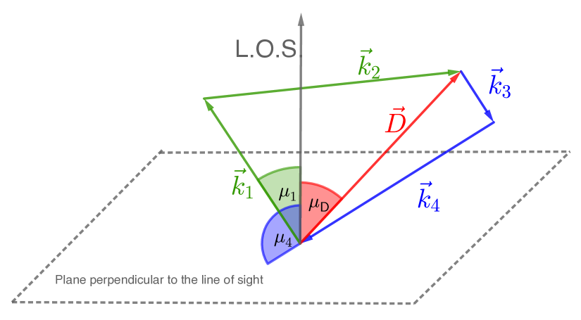
Refer to caption
Figure 12: trispectrum coordinates used to describe each configuration in the analytical model. μD,μ1,μ4subscript𝜇𝐷subscript𝜇1subscript𝜇4\mu_{D},\mu_{1},\mu_{4} are the cosine of the angles between the line of sight and the vectors 𝐃,𝐤1,𝐤4𝐃subscript𝐤1subscript𝐤4\mathbf{D},\mathbf{k}_{1},\mathbf{k}_{4}, respectively.

B.1 Trispectrum integration volume and grid points quadruplets

The key to compute the integration volume for the trispectrum consists in considering one of the two diagonals. By doing so each trispectrum configuration can be described by 8 variables (12 degrees of freedom minus 3 for the Dirac’s delta closure condition minus 1 for the invariance with respect rotations around the line of sight). A good choice for these are the four sides modules (k1,k2,k3,k4)subscript𝑘1subscript𝑘2subscript𝑘3subscript𝑘4\left(k_{1},k_{2},k_{3},k_{4}\right), one of the two diagonals D𝐷D (let’s choose the one defining the triangles k1k2D¯¯subscript𝑘1subscript𝑘2𝐷\overline{k_{1}k_{2}D} and k3k4D¯¯subscript𝑘3subscript𝑘4𝐷\overline{k_{3}k_{4}D} with closure conditions δD(𝐤1+𝐤2𝐃)subscript𝛿𝐷subscript𝐤1subscript𝐤2𝐃\delta_{D}\left(\mathbf{k}_{1}+\mathbf{k}_{2}-\mathbf{D}\right) and δD(𝐤3+𝐤4+𝐃)subscript𝛿𝐷subscript𝐤3subscript𝐤4𝐃\delta_{D}\left(\mathbf{k}_{3}+\mathbf{k}_{4}+\mathbf{D}\right) respectively) and the cosine of three angles with respect to the line of sight (μD,μ1,μ4)subscript𝜇𝐷subscript𝜇1subscript𝜇4\left(\mu_{D},\mu_{1},\mu_{4}\right) for the diagonal 𝐃𝐃\mathbf{D} and the two sides 𝐤1subscript𝐤1\mathbf{k}_{1}, 𝐤4subscript𝐤4\mathbf{k}_{4}. For a visual representation of the choice of coordinates see Figure 12.

All the other details can be obtained using as coordinates the parallel/perpendicular components of the k-vectors with respect to the line of sight. In this way, to fully define the vector, we must specify also the azimuthal angle on the plane perpendicular to the line of sight. This allows us to fully exploit the invariance symmetry related to the rotation of the quadrilateral around the line of sight. This is done by setting the origin of the azimuthal angle to be in the diagonal (γD=0subscript𝛾𝐷0\gamma_{D}=0) and by computing the other four azimuthal angles with respect to it, using the condition that the projection on the perpendicular plane must also be a closed quadrilateral composed by two closed triangles.

Considering the two triangles mentioned above, we start from the diagonal vector 𝐃𝐃\mathbf{D} yielding the initial volume VD4πD2ΔDsimilar-to-or-equalssubscript𝑉𝐷4𝜋superscript𝐷2Δ𝐷V_{D}\simeq 4\pi D^{2}\Delta D. Now we can proceed for each triangle as in the case of the bispectrum integration volume (see Appendix of [48]) obtaining the symmetric final result:

Vq=VD×Vk12×Vk34=16π3k1k2k3k4Δk1Δk2Δk3Δk4ΔD.subscript𝑉qsubscript𝑉𝐷subscript𝑉subscript𝑘12subscript𝑉subscript𝑘3416superscript𝜋3subscript𝑘1subscript𝑘2subscript𝑘3subscript𝑘4Δsubscript𝑘1Δsubscript𝑘2Δsubscript𝑘3Δsubscript𝑘4Δ𝐷\displaystyle V_{\mathrm{q}}=V_{D}\times V_{k_{12}}\times V_{k_{34}}=16\pi^{3}k_{1}k_{2}k_{3}k_{4}\Delta k_{1}\Delta k_{2}\Delta k_{3}\Delta k_{4}\Delta D\,. (B.1)

The number of grid points quadruplets is then defined as Nq=Vqkf9subscript𝑁qsubscript𝑉qsuperscriptsubscript𝑘𝑓9N_{\mathrm{q}}=\dfrac{V_{\mathrm{q}}}{k_{f}^{9}}.

B.2 Tetraspectrum integration volume and grid points quintuplets

For future reference we also include the integration volume for the tetraspectrum. This can be derived using the same trick of splitting the figure into triangles made by the sides and the diagonals. A particular pentagon configuration is described by 11 variables (15 degrees of freedom minus 3 for the Dirac’s delta closure condition minus 1 for the invariance with respect rotations around the line of sight).

Once more we choose the 5 sides modules (k1,k2,k3,k4,k5)subscript𝑘1subscript𝑘2subscript𝑘3subscript𝑘4subscript𝑘5\left(k_{1},k_{2},k_{3},k_{4},k_{5}\right) and two diagonals DAsubscript𝐷𝐴D_{A} and DBsubscript𝐷𝐵D_{B} such that the resulting triangles are DAk2k3¯¯subscript𝐷𝐴subscript𝑘2subscript𝑘3\overline{D_{A}k_{2}k_{3}}, DAk1DB¯¯subscript𝐷𝐴subscript𝑘1subscript𝐷𝐵\overline{D_{A}k_{1}D_{B}} and DBk4k5¯¯subscript𝐷𝐵subscript𝑘4subscript𝑘5\overline{D_{B}k_{4}k_{5}}. Finally we use the four cosine of the angles with respect to the line of sight (μDA,μDB,μ2,μ4)subscript𝜇subscript𝐷𝐴subscript𝜇subscript𝐷𝐵subscript𝜇2subscript𝜇4\left(\mu_{D_{A}},\mu_{D_{B}},\mu_{2},\mu_{4}\right).

The volume can be computed starting from the one for the quadrilateral DBk1k2k3¯¯subscript𝐷𝐵subscript𝑘1subscript𝑘2subscript𝑘3\overline{D_{B}k_{1}k_{2}k_{3}} which is:

VqB123=16π3DBk1k2k3ΔDBΔk1Δk2Δk3.subscriptsuperscript𝑉𝐵123q16superscript𝜋3subscript𝐷𝐵subscript𝑘1subscript𝑘2subscript𝑘3Δsubscript𝐷𝐵Δsubscript𝑘1Δsubscript𝑘2Δsubscript𝑘3\displaystyle V^{B123}_{\mathrm{q}}=16\pi^{3}D_{B}k_{1}k_{2}k_{3}\Delta D_{B}\Delta k_{1}\Delta k_{2}\Delta k_{3}\,. (B.2)

Again applying the bispectrum formula for the triangle DBk4k5¯¯subscript𝐷𝐵subscript𝑘4subscript𝑘5\overline{D_{B}k_{4}k_{5}} we have that:

Vk45=2πk4k5DBΔk4Δk5,subscript𝑉subscript𝑘452𝜋subscript𝑘4subscript𝑘5subscript𝐷𝐵Δsubscript𝑘4Δsubscript𝑘5\displaystyle V_{k_{45}}=2\pi\dfrac{k_{4}k_{5}}{D_{B}}\Delta k_{4}\Delta k_{5}\,, (B.3)

and therefore the tetraspectrum integration volume Vcsubscript𝑉cV_{\mathrm{c}} (’c’ stands for cinco/cinque) can be obtained by simply multiplying

Vc=VqB123×Vk45=32π4k1k2k3k4k5Δk1Δk2Δk3Δk4Δk5ΔDAΔDB.subscript𝑉csubscriptsuperscript𝑉𝐵123qsubscript𝑉subscript𝑘4532superscript𝜋4subscript𝑘1subscript𝑘2subscript𝑘3subscript𝑘4subscript𝑘5Δsubscript𝑘1Δsubscript𝑘2Δsubscript𝑘3Δsubscript𝑘4Δsubscript𝑘5Δsubscript𝐷𝐴Δsubscript𝐷𝐵\displaystyle V_{\mathrm{c}}=V^{B123}_{\mathrm{q}}\times V_{k_{45}}=32\pi^{4}k_{1}k_{2}k_{3}k_{4}k_{5}\Delta k_{1}\Delta k_{2}\Delta k_{3}\Delta k_{4}\Delta k_{5}\Delta D_{A}\Delta D_{B}\,. (B.4)

The number of grid points quintuplets is then defined as Nc=Vckf12subscript𝑁csubscript𝑉csuperscriptsubscript𝑘𝑓12N_{\mathrm{c}}=\dfrac{V_{\mathrm{c}}}{k_{f}^{12}}.

Appendix C Survey window effect on the covariance matrix

In this Appendix we investigate the origin of the features parallel to the main diagonal of the numerically estimated covariance matrix in Figure 3. For this purpose we use the measurements of the same data-vector (power spectrum monopole and quadrupole plus bispectrum monopole) made on simulated cubic boxes with periodic boundary conditions [27]. Because of the fewer number of measurements available (440 with respect to 1400), the bispectrum data-vector contains 47 triangle configurations, less than the 68 employed in Figure 3.

While the overall discrepancy between analytical and numerical estimates is approximately the same as in Figure 3, in the top-right panel of Figure 13 there are no features parallel to the main diagonal. This difference between Figure 3 and Figure 13 supports our hypothesis that those features are not physical but related to the mode-coupling induced by the survey window selection function.
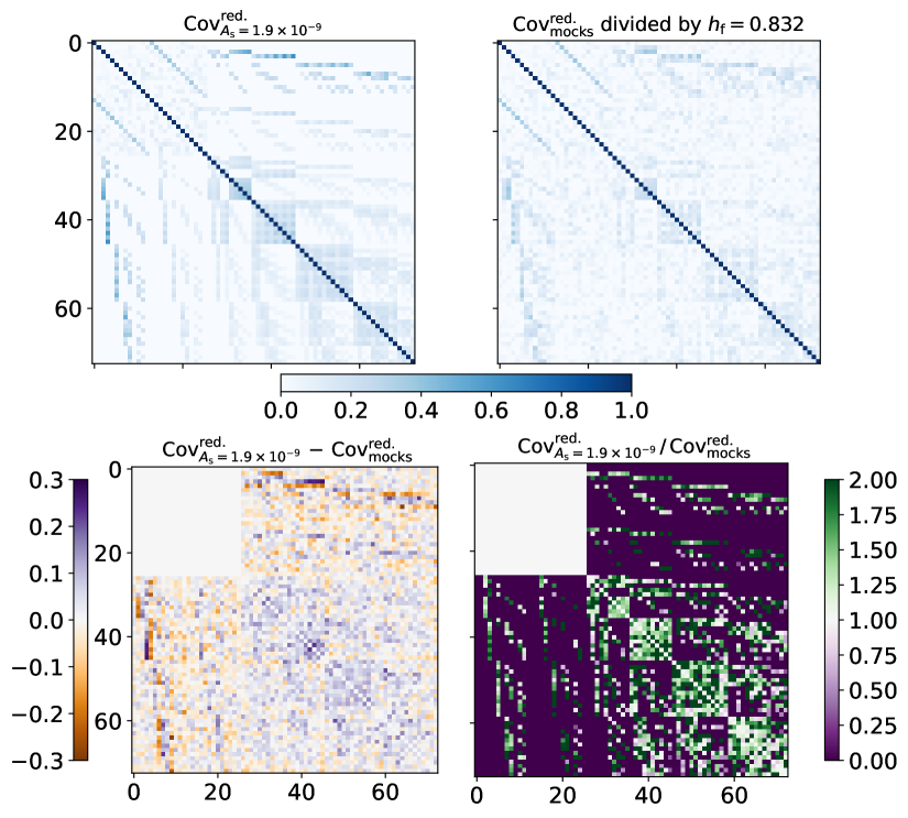
Refer to caption
Figure 13: Same as Figure 3 but with the numerical covariance obtained by measuring the power spectrum (monopole and quadrupole) and bispectrum monopole from a set of 440 simulated cubic volumes with periodic boundary conditions. In Figure 3 we used 1400 measurements from galaxy mock catalogues to estimate the covariance matrix for the bispectrum of 68 triangles configurations. Here we considered 47 triangle configurations to derive the bispectrum covariance from 440 simulated cubic boxes with periodic boundary conditions. The overall discrepancy between the analytical and numerical covariances described in the two bottom panels is qualitatively the same as the one in Figure 3. However in this case where the galaxy field has a regular geometry (cubic box with side L=5000h/L=5000\,h/Mpc ) and therefore no survey window selection effect, those features parallel to the main diagonal present in Figure 3 are here absent. Therefore this test corroborates our hypothesis of those features being related to the mode-coupling induced by the survey window selection effect.

Appendix D 𝚫𝐤𝟔𝚫subscript𝐤6\mathbf{\Delta k_{6}} binning case figures

This last Appendix contains the two key figures and improvements table for the Δk6Δsubscript𝑘6\Delta k_{6} binning case.

Refer to caption
Figure 14: Same as Figure 5 for the Δk6Δsubscript𝑘6\Delta k_{6} binning case.
Refer to caption
Figure 15: Same as Figure 10 for the Δk6Δsubscript𝑘6\Delta k_{6} binning case.
statistics ΔθPg(0,2);Bg(00)num.cov.ΔθPg(0,2);Bg(ı,ȷ)hyb.cov.ΔθPg(0,2);Bg(00)num.cov.[%]\dfrac{\Delta\theta^{\mathrm{num.\,cov.}}_{\mathrm{P_{g}^{(0,2)};B_{g}^{(00)}}}-\Delta\theta^{\mathrm{hyb.\,cov.}}_{\mathrm{P_{g}^{(0,2)};B_{g}^{(\imath,\jmath)}}}}{\Delta\theta^{\mathrm{num.\,cov.}}_{\mathrm{P_{g}^{(0,2)};B_{g}^{(00)}}}}\;\left[\%\right]
Pg(0,2)+limit-fromsuperscriptsubscriptPg02\mathrm{P}_{\mathrm{g}}^{(0,2)}\;+ b1subscript𝑏1b_{1} b2subscript𝑏2b_{2} f𝑓f σ8subscript𝜎8\sigma_{8} fNLsubscript𝑓NLf_{\mathrm{NL}} αsubscript𝛼parallel-to\alpha_{\parallel} αsubscript𝛼perpendicular-to\alpha_{\perp} average
Bg(00)superscriptsubscriptBg00\mathrm{\mathrm{B}_{\mathrm{g}}^{(00)}} 2.4 3.4 -4.9 2.9 2.0 0.6 -5.5 0.1
Bg(00,20)superscriptsubscriptBg0020\mathrm{\mathrm{B}_{\mathrm{g}}^{(00,20)}} 46.8 53.6 39.4 31.1 37.6 43.0 42.8 42.0
Bg(00,20,02)superscriptsubscriptBg002002\mathrm{\mathrm{B}_{\mathrm{g}}^{(00,20,02)}} 55.8 61.5 49.6 43.0 44.0 50.1 45.0 49.9
Bg(00,20,02,40)superscriptsubscriptBg00200240\mathrm{\mathrm{B}_{\mathrm{g}}^{(00,20,02,40)}} 55.3 61.2 51.1 41.5 44.2 52.7 46.7 50.4
Bg(00,20,02,40,04)superscriptsubscriptBg0020024004\mathrm{\mathrm{B}_{\mathrm{g}}^{(00,20,02,40,04)}} 57.8 63.1 56.9 45.4 49.8 59.6 50.8 54.8
Bg(00,20,02,40,04,22)superscriptsubscriptBg002002400422\mathrm{\mathrm{B}_{\mathrm{g}}^{(00,20,02,40,04,22)}} 57.1 62.8 57.0 44.0 51.9 60.2 52.6 55.1
Table 3: Same as Table 2 for the Δk6Δsubscript𝑘6\Delta k_{6} binning case. The table tells us that even if the average improvement is larger with respect to the Δk5Δsubscript𝑘5\Delta k_{5} binning case, the information gain reaches saturation always at the bispectrum hexadecapole level. At the same time if we compare the 1-2D marginalised posterior distributions shown in Figures 10 and 15 for the Δk5Δsubscript𝑘5\Delta k_{5} and Δk6Δsubscript𝑘6\Delta k_{6} cases respectively, we can see that once all the hexadecapole terms have been added to the data vector, the width of the contours is similar.

Acknowledgments

D.G. thanks Héctor Gil Marín for providing the data vector’s measurements from the galaxy mocks and for useful discussions. D.G. and L.V. are very grateful to Cheng Zhao and Chia-Hsun Chuang for the periodic simulations used to test the survey window effect on the covariance. L.V. and D.G. acknowledge support of European Unions Horizon 2020 research and innovation programme ERC (BePreSySe, grant agreement 725327). Funding for this work was partially provided by the Spanish Ministerio de Ciencia y Innovation y Universidades under project PGC2018-098866-B-I00.

References

  • Aghanim et al. [2018] Aghanim N., et al., 2018
  • Akrami et al. [2019] Akrami Y., et al., 2019
  • Alam et al. [2015] Alam S., et al., 2015, Astrophys. J. Suppl., 219, 12
  • Alam et al. [2017] Alam S., et al., 2017, Mon. Not. Roy. Astron. Soc., 470, 2617
  • Alcock & Paczynski [1979] Alcock C., Paczynski B., 1979, Nature, 281, 358
  • Baldauf et al. [2011] Baldauf T., Seljak U., Senatore L., 2011, JCAP, 1104, 006
  • Baldauf et al. [2012] Baldauf T., Seljak U., Desjacques V., McDonald P., 2012, Phys. Rev., D86, 083540
  • Bardeen [1980] Bardeen J. M., 1980, Phys. Rev., D22, 1882
  • Barreira [2019] Barreira A., 2019, JCAP, 1903, 008
  • Bartolo et al. [2004] Bartolo N., Komatsu E., Matarrese S., Riotto A., 2004, Phys. Rept., 402, 103
  • Bartolo et al. [2013] Bartolo N., Bellini E., Bertacca D., Matarrese S., 2013, JCAP, 1303, 034
  • Bellini et al. [2015] Bellini E., Jimenez R., Verde L., 2015, JCAP, 1505, 057
  • Bernardeau et al. [2002] Bernardeau F., Colombi S., Gaztanaga E., Scoccimarro R., 2002, Phys. Rept., 367, 1
  • Bertacca et al. [2018] Bertacca D., Raccanelli A., Bartolo N., Liguori M., Matarrese S., Verde L., 2018, Phys. Rev., D97, 023531
  • Beutler et al. [2014] Beutler F., et al., 2014, Mon. Not. Roy. Astron. Soc., 443, 1065
  • Beutler et al. [2017] Beutler F., et al., 2017, Mon. Not. Roy. Astron. Soc., 466, 2242
  • Blake et al. [2018] Blake C., Carter P., Koda J., 2018, Mon. Not. Roy. Astron. Soc., 479, 5168
  • Bose & Taruya [2018] Bose B., Taruya A., 2018, JCAP, 1810, 019
  • Brinckmann et al. [2019] Brinckmann T., Hooper D. C., Archidiacono M., Lesgourgues J., Sprenger T., 2019, JCAP, 1901, 059
  • Byrnes & Choi [2010] Byrnes C. T., Choi K.-Y., 2010, Adv. Astron., 2010, 724525
  • Byun & Bean [2013] Byun J., Bean R., 2013, JCAP, 1309, 026
  • Byun et al. [2017] Byun J., Eggemeier A., Regan D., Seery D., Smith R. E., 2017, Mon. Not. Roy. Astron. Soc., 471, 1581
  • Carron [2013] Carron J., 2013, Astron. Astrophys., 551, A88
  • Castiblanco et al. [2019] Castiblanco L., Gannouji R., Noreña J., Stahl C., 2019, JCAP, 1907, 030
  • Castorina et al. [2019] Castorina E., et al., 2019, JCAP, 1909, 010
  • Chan et al. [2012] Chan K. C., Scoccimarro R., Sheth R. K., 2012, Phys. Rev., D85, 083509
  • Chuang et al. [2015] Chuang C.-H., Kitaura F.-S., Prada F., Zhao C., Yepes G., 2015, Mon. Not. Roy. Astron. Soc., 446, 2621
  • Colas et al. [2019] Colas T., D’amico G., Senatore L., Zhang P., Beutler F., 2019
  • Coulton et al. [2019] Coulton W. R., Liu J., Madhavacheril M. S., Böhm V., Spergel D. N., 2019, JCAP, 1905, 043
  • Dalal et al. [2008] Dalal N., Dore O., Huterer D., Shirokov A., 2008, Phys. Rev. D, 77, 123514
  • Desjacques et al. [2018] Desjacques V., Jeong D., Schmidt F., 2018, JCAP, 1812, 035
  • Di Dio et al. [2019] Di Dio E., Durrer R., Maartens R., Montanari F., Umeh O., 2019, JCAP, 1904, 053
  • Eggemeier et al. [2019] Eggemeier A., Scoccimarro R., Smith R. E., 2019, Phys. Rev., D99, 123514
  • Eisenstein et al. [2011] Eisenstein D. J., et al., 2011, Astron. J., 142, 72
  • Figueroa et al. [2012] Figueroa D. G., Sefusatti E., Riotto A., Vernizzi F., 2012, JCAP, 1208, 036
  • Fry [1984] Fry J. N., 1984, Astrophys. J., 279, 499
  • Fry [1994] Fry J. N., 1994, Astrophys. J., 421, 21
  • Fry & Gaztanaga [1993] Fry J. N., Gaztanaga E., 1993, Astrophys. J., 413, 447
  • Fry & Seldner [1982] Fry J. N., Seldner M., 1982, ApJ, 259, 474
  • Gagrani & Samushia [2017] Gagrani P., Samushia L., 2017, Mon. Not. Roy. Astron. Soc., 467, 928
  • Giannantonio & Porciani [2010] Giannantonio T., Porciani C., 2010, Phys. Rev. D, 81, 063530
  • Gil-Marin et al. [2011] Gil-Marin H., Schmidt F., Hu W., Jimenez R., Verde L., 2011, JCAP, 1111, 019
  • Gil-Marín et al. [2015] Gil-Marín H., Noreña J., Verde L., Percival W. J., Wagner C., Manera M., Schneider D. P., 2015, Mon. Not. Roy. Astron. Soc., 451, 539
  • Gil-Marín et al. [2017] Gil-Marín H., Percival W. J., Verde L., Brownstein J. R., Chuang C.-H., Kitaura F.-S., Rodríguez-Torres S. A., Olmstead M. D., 2017, Mon. Not. Roy. Astron. Soc., 465, 1757
  • Groth & Peebles [1977] Groth E. J., Peebles P. J. E., 1977, Astrophys. J., 217, 385
  • Gualdi et al. [2018] Gualdi D., Manera M., Joachimi B., Lahav O., 2018, Mon. Not. Roy. Astron. Soc., 476, 4045
  • Gualdi et al. [2019a] Gualdi D., Gil-Marín H., Manera M., Joachimi B., Lahav O., 2019a
  • Gualdi et al. [2019b] Gualdi D., Gil-Marín H., Schuhmann R. L., Manera M., Joachimi B., Lahav O., 2019b, Mon. Not. Roy. Astron. Soc., 484, 3713
  • Hahn et al. [2019] Hahn C., Francisco V.-N., Emanuele C., Roman S., 2019
  • Hamilton [1997] Hamilton A. J. S., 1997, in Ringberg Workshop on Large Scale Structure Ringberg, Germany, September 23-28, 1996. (arXiv:astro-ph/9708102), doi:10.1007/978-94-011-4960-0_17
  • Hartlap et al. [2006] Hartlap J., Simon P., Schneider P., 2006, Astron. Astrophys.
  • Hashimoto et al. [2017] Hashimoto I., Rasera Y., Taruya A., 2017, Phys. Rev., D96, 043526
  • Hinshaw et al. [2003] Hinshaw G., et al., 2003, Astrophys. J. Suppl., 148, 135
  • Ivanov et al. [2019b] Ivanov M. M., Simonović M., Zaldarriaga M., 2019b
  • Ivanov et al. [2019a] Ivanov M. M., Simonović M., Zaldarriaga M., 2019a
  • Jackson [1972] Jackson J. C., 1972, Mon. Not. Roy. Astron. Soc., 156, 1P
  • Jeong & Komatsu [2009] Jeong D., Komatsu E., 2009, Astrophys. J., 703, 1230
  • Joachimi et al. [2009] Joachimi B., Shi X., Schneider P., 2009, Astron. Astrophys., 508, 1193
  • Kaiser [1987] Kaiser N., 1987, Mon. Not. Roy. Astron. Soc., 227, 1
  • Karagiannis et al. [2018] Karagiannis D., Lazanu A., Liguori M., Raccanelli A., Bartolo N., Verde L., 2018, Mon. Not. Roy. Astron. Soc., 478, 1341
  • Kitaura et al. [2016] Kitaura F.-S., et al., 2016, Mon. Not. Roy. Astron. Soc., 456, 4156
  • Komatsu & Spergel [2001] Komatsu E., Spergel D. N., 2001, Phys. Rev., D63, 063002
  • Lesgourgues [2011] Lesgourgues J., 2011
  • Liguori et al. [2010] Liguori M., Sefusatti E., Fergusson J. R., Shellard E. P. S., 2010, Adv. Astron., 2010, 980523
  • Matarrese & Verde [2008] Matarrese S., Verde L., 2008, Astrophys. J. Lett., 677, L77
  • Matarrese et al. [1997] Matarrese S., Verde L., Heavens A. F., 1997, Mon. Not. Roy. Astron. Soc., 290, 651
  • Montesano et al. [2010] Montesano F., Sanchez A. G., Phleps S., 2010, Mon. Not. Roy. Astron. Soc., 408, 2397
  • Montesano et al. [2012] Montesano F., Sanchez A. G., Phleps S., 2012, Mon. Not. Roy. Astron. Soc., 421, 2656
  • Oddo et al. [2019] Oddo A., Sefusatti E., Porciani C., Monaco P., Sánchez A. G., 2019
  • Peebles & Groth [1975] Peebles P. J. E., Groth E. J., 1975, ApJ, 196, 1
  • Perotto et al. [2006] Perotto L., Lesgourgues J., Hannestad S., Tu H., Wong Y. Y. Y., 2006, JCAP, 0610, 013
  • Philcox et al. [2020] Philcox O. H. E., Ivanov M. M., Simonović M., Zaldarriaga M., 2020
  • Repp et al. [2015] Repp A., Szapudi I., Carron J., Wolk M., 2015, Mon. Not. Roy. Astron. Soc., 454, 3533
  • Rodríguez-Torres et al. [2016] Rodríguez-Torres S. A., et al., 2016, Mon. Not. Roy. Astron. Soc., 460, 1173
  • Ruggeri et al. [2018] Ruggeri R., Castorina E., Carbone C., Sefusatti E., 2018, JCAP, 1803, 003
  • Scoccimarro [2015] Scoccimarro R., 2015, Phys. Rev., D92, 083532
  • Scoccimarro & Couchman [2001] Scoccimarro R., Couchman H. M. P., 2001, Mon. Not. Roy. Astron. Soc., 325, 1312
  • Scoccimarro et al. [1998] Scoccimarro R., Colombi S., Fry J. N., Frieman J. A., Hivon E., Melott A., 1998, Astrophys. J., 496, 586
  • Scoccimarro et al. [1999a] Scoccimarro R., Couchman H. M. P., Frieman J. A., 1999a, Astrophys. J., 517, 531
  • Scoccimarro et al. [1999b] Scoccimarro R., Zaldarriaga M., Hui L., 1999b, Astrophys. J., 527, 1
  • Scoccimarro et al. [2001] Scoccimarro R., Feldman H. A., Fry J. N., Frieman J. A., 2001, Astrophys. J., 546, 652
  • Scoccimarro et al. [2004] Scoccimarro R., Sefusatti E., Zaldarriaga M., 2004, Phys. Rev., D69, 103513
  • Sefusatti [2009] Sefusatti E., 2009, Phys. Rev., D80, 123002
  • Sefusatti & Scoccimarro [2005] Sefusatti E., Scoccimarro R., 2005, Phys. Rev., D71, 063001
  • Sefusatti et al. [2006] Sefusatti E., Crocce M., Pueblas S., Scoccimarro R., 2006, Phys. Rev., D74, 023522
  • Sefusatti et al. [2012] Sefusatti E., Crocce M., Desjacques V., 2012, Mon. Not. Roy. Astron. Soc., 425, 2903
  • Slepian et al. [2017] Slepian Z., et al., 2017, Mon. Not. Roy. Astron. Soc., 468, 1070
  • Sugiyama et al. [2019a] Sugiyama N. S., Saito S., Beutler F., Seo H.-J., 2019a
  • Sugiyama et al. [2019b] Sugiyama N. S., Saito S., Beutler F., Seo H.-J., 2019b, Mon. Not. Roy. Astron. Soc., 484, 364
  • Tellarini et al. [2015] Tellarini M., Ross A. J., Tasinato G., Wands D., 2015, JCAP, 07, 004
  • Tellarini et al. [2016] Tellarini M., Ross A. J., Tasinato G., Wands D., 2016, JCAP, 06, 014
  • Verde et al. [1998] Verde L., Heavens A. F., Matarrese S., Moscardini L., 1998, Mon. Not. Roy. Astron. Soc., 300, 747
  • Verde et al. [2000] Verde L., Wang L.-M., Heavens A., Kamionkowski M., 2000, Mon. Not. Roy. Astron. Soc., 313, L141
  • Verde et al. [2002] Verde L., et al., 2002, Mon. Not. Roy. Astron. Soc., 335, 432
  • Wadekar & Scoccimarro [2019] Wadekar D., Scoccimarro R., 2019
  • Yankelevich & Porciani [2019] Yankelevich V., Porciani C., 2019, Mon. Not. Roy. Astron. Soc., 483, 2078
  • Zheng et al. [2019] Zheng J., Zhao G.-B., Li J., Wang Y., Chuang C.-H., Kitaura F.-S., Rodriguez-Torres S., 2019, Mon. Not. Roy. Astron. Soc., 484, 442