Quantitative assessment of the role of undocumented infection in the 2019 novel coronavirus (COVID-19) pandemic
An urgent problem in controlling COVID-19 spreading is to understand the role of undocumented infection. We develop a five-state model for COVID-19, taking into account the unique features of the novel coronavirus, with key parameters determined by the government reports and mathematical optimization. Tests using data from China, South Korea, Italy, and Iran indicate that the model is capable of generating accurate prediction of the daily accumulated number of confirmed cases and is entirely suitable for real-time prediction. The drastically disparate testing and diagnostic standards/policies among different countries lead to large variations in the estimated parameter values such as the duration of the outbreak, but such uncertainties have little effect on the occurrence time of the inflection point as predicted by the model, indicating its reliability and robustness. Model prediction for Italy suggests that insufficient government action leading to a large fraction of undocumented infection plays an important role in the abnormally high mortality in that country. With the data currently available from United Kingdom, our model predicts catastrophic epidemic scenarios in the country if the government did not impose strict travel and social distancing restrictions. A key finding is that, if the percentage of undocumented infection exceeds a threshold, a non-negligible hidden population can exist even after the the epidemic has been deemed over, implying the likelihood of future outbreaks should the currently imposed strict government actions be relaxed. This could make COVID-19 evolving into a long-term epidemic or a community disease a real possibility, suggesting the necessity to conduct universal testing and monitoring to identify the hidden individuals.
Introduction
At the end of December 2019, an unexplained, new type of coronavirus emerged in the city of Wuhan in Hubei province of China. On January 10, 2020, the health officials of Wuhan city confirmed, through nucleic acid detection, 41 cases. Coincided with ChunYun, the annual period of mass migration in China for the Spring Festival holidays, the virus began to spread from Wuhan city to other regions of China. On January 23, 2020, the Health Department of the Central Chinese Government locked down Wuhan, a city of 11 millions, and a number of other cities and regions in Hubei province, and at the same time implemented rigorous, nationwide travel restrictions, in an attempt to prevent large scale spreading of the disease (?). In spite of the strict measures, suspected and confirmed cases began to emerge in almost every province and major city of China, with a rapid increase in a short time period. On February 11, 2020, the International Committee on Taxonomy of Viruses designated the virus as severe acute respiratory syndrome coronavirus 2 (SARS-CoV-2) and on the same day, the World Health Organization (WHO) officially named the disease as COVID-19. The unprecedented, rigorous measures imposed by the Central Chinese Government have proven to be quite effective at controlling and suppressing the spread, stabilizing its dynamics. At the time of writing, there were only a few newly confirmed cases in China. While spreading in China has apparently diminished, SARS-CoV-2 has begun to emerge in counties and regions outside China, with large scale spreading in South Korea, Italy, Iran, and now in the United States. With the likelihood that COVID-19 would become a catastrophe in public health, on February 28 WHO has raised the global risk level of the new corona pneumonia epidemic from “high” to “very high.” On March 11, WHO declared COVID-19 a global pandemic.
For COVID-19, a number of data analysis studies have provided estimates of the basic parameters underlying the spreading dynamics. In particular, the very first 425 confirmed cases were analyzed (?) with the findings that the average incubation period was 5.2 days, the doubling time was about 7.4 days and the basic reproduction number was about 2.2 extracted from the exponential growth behavior, and the infection due to personal contacts had already occurred. An analysis (?) of the 72314 confirmed cases in China up to February 11, 2020 found 889 asymptomatic cases (about ) and 1023 deaths (). From the growth curve, it was extrapolated that the epidemic in China would peak about January 23-26. An analysis of a data base of large number of samples revealed (?) the median incubation period of about four days, quartile of five days (two-seven days), and death rate about . According to the joint China-WHO Joint Investigation Report on New Crown Pneumonia, the median time interval between symptom appearance and confirmation in China was 12 days (8-18 days) in January and reduced to three days (1-7 days) at the beginning of February, but in Wuhan the respective numbers are 15 days (10-21 days) and five days (3-9 days). Initial usable data indicated that, the median time between mild symptoms and cure was about two weeks, while that between severe symptoms and cure was between three and six weeks, and it took about one week to go from initial symptoms to severe illness such as hypoxia. Among the cases who did not survive, the time from initial symptoms to death was between two and eight weeks. There are similarities between SARS-CoV-2 and SARS-Cov (Severe Acute Respiratory Syndrome associated Coronavirus) or MERS-Cov (Middle East Respiratory Syndrome associated Coronavirus), but there are also differences (?). While the propagation scenarios among the three viruses are similar, the rapid spreading in China and evidence of infection through human-to-human contacts suggested that SARS-CoV-2 is more infectious than SARS-Cov or MERS-Cov, and the strong infectability during the relatively long incubation period is particularly worrisome (?). These features of SARS-CoV-2, in spite of the associated relatively small death rate, can cause more damage to the society, posing a significant challenge to control, mitigation, and prevention.
For virus spreading, developing an effective mathematical model for making reliable predictions is of paramount importance to quantitatively assessing the epidemic trend as well as to control and prevention. In dealing with recent viruses of worldwide impact such as SARS-Cov (?), MERS-Cov (?), Ebola (?) and ZiKa (?) viruses, the modeling approach played an indispensable role. For COVID-19, an SEIR (Susceptible-Exposed-Infectious-Recovered) model was developed (?) based on the OAG (Official Aviation Guide) data, the inter-city population movement data from Tencent, and parameters values with the incubation and infectious periods taken from SARS-CoV. Utilizing cases outside of China, which were originated from Wuhan, to inversely deduce the epidemic spreading process in major cities in China, the authors (?) estimated the value to be 2.68 and the doubling time of 6.4 days. Further, it was predicted that by January 25, 2020, the number of infected cases in Wuhan would be 75,815. This model is quite effective, but two main deficiencies stood: the relevant parameter values were from the previous epidemic of SARS-CoV and, the infectability during the incubation period, perhaps the most distinct feature of SARS-CoV-2, was not taken into account. The SEIR model was also used with parameter values from People’s Daily (the official Central Chinese Government newspaper) to estimate the value based on the initial exponential growth (?), with the result . Another study (?) based on the population movement data from Tencent and Baidu carried out a statistical analysis of the geographic distribution of the population exiting Wuhan, giving an assessment of the impact of this type of population on the epidemic. An improved SEIR model (?) taking into account the infectability during the incubation period and incorporating machine learning trained based on the data from 2003 SARS-CoV, predicted that the epidemic in China would peak in the second half of February and stabilize at the end of April. A remarkable result (?) was that, should the Central Government’s rigorous quarantine and control measures be delayed for five days, the size of the epidemic in China would be tripled and, if the lockdown measures of Wuhan were relaxed, a second peak would emerge and last through the second half of April. An assumption in this model was that the incubation time distribution is Markovian, i.e., the occurrence time of the transition from incubation to being infected follows the Poisson distribution with exponentially distributed interevent time. However, for COVID-19, the assumed Markovian spreading process is too idealized, as there were substantial empirical data (?) indicating that the incubation period of COVID-19 has a strong non-Markovian characteristic, i.e., there is a time delay between incubation and appearance of symptoms. A delayed spreading model incorporating the non-Markovian characteristics was then developed (?), taking into account the city lockdown and using an inverse approach for parameter estimation, which predicted the infection rate for mainland China of about 0.23 and isolation rate of about 0.42. A difficulty is that the current isolation measures in China were implemented in response to the development of the epidemic, which are time-dependent and may even be temporal. It has been predicted (?) that, had the implementation of the government control measures been delayed for five days, the epidemic scale in mainland China would have been three times larger. The effects of travel restrictions in China on global COVID-19 spreading have also been studied (?).
While the recent studies (?, ?, ?, ?, ?, ?, ?, ?, ?) provided useful insights into the COVID-19 pandemic, three significant characteristics were not taken into account: (1) the existence of a non-zero fraction of hidden and undocumented individuals who carry the virus but are asymptomatic during incubation, mildly symptomatic, or even never symptomatic, (2) non-Markovian features associated with state transitions during the epidemic, and (3) the effects of time-dependent activities associated with population movements and contacts. The models constructed so far without taking into these key features generated parameter estimates that deviate from those of the real spreading dynamics, with incorrect predictions about the epidemic dynamics and trend. While the government provides the numbers of the newly confirmed and accumulated cases on a daily basis, it is impossible to know the accurate number of the hidden individuals who are infectious but have not been isolated or quarantined. These individuals are precisely the single most important factor for possible future outbreaks. Indeed, a very recent study (?) revealed that substantial undocumented infection tends to facilitate the rapid spreading of COVID-19 as has been witnessed in many countries. There was speculation of the possibility of COVID-19 evolving into a community disease and a long term epidemic but there has been no supporting evidence so far. If, after the current epidemic is over, the fraction of virus carrying individuals in incubation approaches zero, then the likelihood for a future outbreak would be very low. However, the alternative devastating scenario could arise: if the fraction is nonzero and persists after the current pandemic, the danger of a new outbreak and COVID-19 becoming a community disease would be real, and this would have indescribable consequences to the whole world. The main goal of our work is to provide quantitative evidence to either support or reject this scenario.
In this paper, we develop a five-state, non-Markovian spreading model for COVID-19 incorporating the time delays associated with various state transitions. The individuals who are asymptomatic are viewed as an important reason for the currently ongoing large scale spreading. In addition, the non-Markovian characteristics associated with state transitions and the time-dependent variations in the human activities under the rigorous governmental actions of isolation, quarantine, and travel restrictions are fully accounted for. Simulations indicate that our model is capable of accurately predicting the epidemic trend in China, South Korea, Italy, and Iran. In fact, the large variations in the estimated number of the undocumented individuals in different countries due to the disparity in government actions have no effect on the predicted occurrence time of the inflection point. Our model provides an explanation for the abnormally high mortality in Italy. Based on the currently available data, our model predicts catastrophic epidemic scenarios in United Kingdom without strict travel and social distancing restrictions. As the number of confirmed cases approaches zero, the seemingly quiescent state may justify relaxation of the currently rigorously enforced quarantine policies (e.g., in China). However, such relaxation can lead to an increase in the fraction of hidden and undocumented individuals. Our model predicts that, if this fraction exceeds a certain value, the epidemic duration can increase by as long as two months, rendering likely a future outbreak. Another prediction is that the decay of the hidden population can be slower than that of the infected one and can maintain at a small but non-zero value for an extended period of time, and this has potentially devastating consequences: the activities of these individuals in combination with the unusually strong virulence of SARS-CoV-2 imply that they are a “time bomb” for a large scale outbreak in the future. The prolonged existence of the hidden/undocumented individuals makes COVID-19 evolving into a long term epidemic and a community disease a real possibility. Our findings provide the base for articulating and implementing further government actions, e.g., universal testing and monitoring to uncover and identify the individuals in the hidden state, to prevent future outbreaks.
Model and parameter estimation
Five-state model
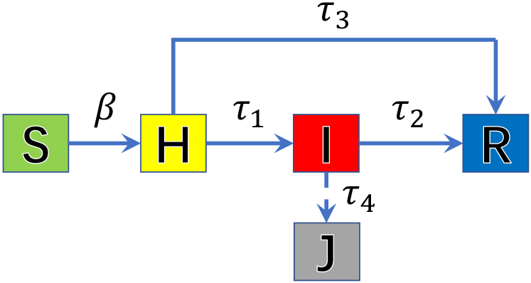
At each time step, an individual can be in one of the five states: susceptible (S), hidden (H), infected (I), confirmed and isolated (J), and recovered (R). An individual in S is healthy but can be infected. An individual in H carries the virus but is asymptomatic or mildly symptomatic, and he/she can infect other individuals. There are two types of individuals in the H state: those who are quarantined and those who are not. Individuals in the I state have been infected and exhibit symptoms. A fraction of the infected population have been confirmed and hospitalized, to which we designate a new state, J. Finally, individuals in the R state are either recovered or died of the disease. Because of the strong government actions, the infected individuals are fully aware of their state and are either quarantined or self-isolated; these individuals thus would not spread the virus, which is especially true for those in the J state who are in hospitals. Likewise, individuals in the R state are not infectious. Thus, in our model, only the individuals in the H state are able to infect others to spread the virus. Note that, one could define the H state as one that contains the asymptomatic individuals and those who are symptomatic but have not been identified. In this case, the duration of the H state consists of the medical incubation period (from the time of infection to the time of symptoms) and the time taken to isolation, while the I state contains symptomatic and isolated individuals with a time between isolation and confirmation. The distributions of the H and I time can be obtained from empirical data.
The spreading dynamics are illustrated schematically in Fig. 1. The susceptible individuals are infected at rate by those in the H state who are not isolated. The S individuals who have been infected switch to state H. Among the individuals in the H state, a fraction can recover spontaneously through their own immune system or die, a process that requires days. (Parameter is thus the fraction of undocumented cases.) The remaining fraction of the H state individuals exhibit symptoms and switch to the I state after an average incubation period of days, due to the non-Markovian nature of symptom appearances. Individuals in the I state are subject to medical treatment and will either recover or die after days - the average time for the transition from I to R states. A unique feature of our model is the introduction of the J state: on average the I individuals will need days to be confirmed. Mathematically, these processes can be described by the following set of time-delayed dynamical equations:
| (1) | |||||
| (2) | |||||
| (3) | |||||
| (4) | |||||
| (5) |
where is the growth rate of the H-state population and is the number of hidden individuals in the H state who have not been quarantined with quantifying the travel activity level of the population which decays exponentially with time [See Supplementary Information (SI)]. The quantities , , and are probability distributions of the incubation period (), of the treatment time (), of the self-healing time period for the hidden individuals (), and of the time period for an infected individual to be diagnosed (), respectively. The distribution functions are assumed to be normal (?): for , with and denoting the mean and standard deviation of the distribution, respectively.
In Eq. (2), the first term on the right-hand side is the inflow rate of the number of newly emerged individuals in the H state, the second (third) term represents the outflow rate from the H state of the individuals who have been hidden for time to the I (R) state, and the fourth (fifth) term is the outflow rate of the individuals who are initially in the H state and switch to the I (R) state. For Eq. (3), the first term on the right side is the inflow rate of individuals from the H state to the I state, the second term denotes the outflow rate of the new individuals in the H state switching to the I state after time and then to the R state after time , the third term represents the inflow rate of the individuals initially in the H state into the I state, the fourth term is the outflow rate of the individuals who are initially in the H-state, switch to the I state after time , and then change to the R state after time , and the fifth term represents the outflow rate of the individuals who are initially in the I state and are recovered after time . The various terms in Eqs. (4) and (5) can be interpreted in a similar way.
Inference of model parameter values
Based on the joint China-WHO Joint Investigation Report on New Coronavirus Pneumonia and Ref. (?), we set the average incubation period to , the average time from infection to recovery () to be . For the value of the fraction of undocumented infection, due to the variations among different countries in terms of the criteria for testing and confirming infected cases and because of the difficulty to measure this parameter, we make a reasonable assumption about its value. Likewise, because of the lack of empirical data to assess the average time of spontaneous recovery, we exploit the fact that these individuals are more immune to SARS-CoV-2 than the average population and accordingly set . From empirical data, we have , but it has little effect on the dynamics.
In addition to , which other model parameters are key to the current spreading dynamics of COVID-19, subject to government actions? The following features of COVID-19: long hidden time, strong virulence, mild symptoms for many individuals, and difficulty in detecting the SARS-CoV-2 virus, strongly suggest that the population in the H state are mainly responsible for spreading the disease. In addition, the direct impact of the government actions is an exponential reduction in the human movement activities. The parameters , , and are thus key, which can be estimated based on the relatively accurate daily number of the confirmed cases as reported by the governments. In particular, the values of the three parameters can be inferred from the following least squares optimization method:
| (6) |
We use the Levenberg-Marquardt (LM) method (?, ?, ?) to solve (6) to obtain the optimal values , , and .
Results
Determining key model parameters for different countries
| Fit for 25 days (China) | Global optimal (China) | Korea | Italy | Iran | |
| 0.38 | 0.37 | 0.27 | 0.29 | 0.31 | |
| 460 | 525 | 91 | 35 | 800 | |
| 0.16 | 0.15 | 0.18 | 0.18 | 0.18 |
Table 1 lists the values of the three key model parameters: , , and , for five different countries, where for China and for South Korea, Italy, and Iran. Another important parameter is the fraction of undocumented infection that reflects on the effectiveness of the government actions. The ways by which these parameters are obtained differ for different countries. In China, the value of has been officially announced: . For South Korea, Italy, and Iran, no official report of the value of is available, so we simulate the model for both small and large values of . For a given value of , the optimal values of , , and are obtained through the LM optimization method (6) in combination with integration of Eqs. (1-5).
To explain the meaning of parameter , we take China as an example. The lockdown of Wuhan and other cities in the Hubei province occurred on January 23. There were 12 days of active travel: between January 11 and 22. The travel activity function is thus given by
| (7) |
where . Since the spreading dynamics in China was triggered by the human outflow from Wuhan, with the implementation of the strict governmental control measures nationwide, virus spreading in cities other than Wuhan can be neglected. We thus have the total number of individuals participating in the spreading dynamics as millions. Because of the lockdown of Wuhan, the human activity function decreases exponentially but it cannot be zero. We thus set to be (a small constant) for days after the lockdown.
Prediction for China
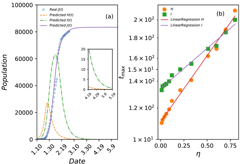
We first demonstrate that our five-state model has the power to accurately predict the epidemic trend of COVID-19 spreading in China in a detailed and quantitative way, and present a striking finding. From the data of COVID-19 spreading in China, we set January 10, 2020 to be the reference time () with the initial conditions , , and . With the estimated parameter values and the initial conditions, we numerically solve the set of delay differential equations Eqs. (1-5). Figure 2(a) shows, in a 100-day period (from January 10 to April 29), the predicted daily accumulated number of confirmed cases (the purple curve) and the available actual data to date (open blue circles). The agreement is remarkable, attesting to the predictive power of our model. Figure 2(a) also shows the predicted daily numbers of the I-state (green dot-dashed curve) and H-state (orange dashed curve) individuals. It can be seen that the epidemic peaked on February 7-8, indicating the occurrence of the inflection point. However, since the average time interval between infection and confirmation is , the observed occurrence of the inflection point would be delayed by , i.e., February 14-15, which was indeed the time reported by the Chinese government. The epidemic cycle is predicted to end towards the end of March when the number of infected individuals approaches zero, which agrees with the currently observed epidemic trend in China.
The above prediction of the epidemic trend in China in terms of and is based on the choice , i.e., among all the H-state individuals, only are undetected and spontaneously recovered or died eventually, which is reasonable, considering the extremely strict monitoring and quarantine policies currently in place in China. If the government actions were not that strict or it they were not rigorously enforced, the value of could be much larger. In that case, how long will the epidemic last? Our model was designed to answer such important questions. Figure 2(b) shows the number of days of the epidemic cycle, defined as the time required for to approach zero, versus , where an approximately exponential relationship is observed. It can be seen that, if the value of is , the epidemic duration could be 200 days. This means that, had the Chinese government not taken the unprecedentedly dramatic steps to contain the COVID-19 spreading, the epidemic cycle could easily last into the summer. Figure 2(b) also shows the model predicted time required for the hidden, virus-carrying population to vanish versus , which is also approximately exponential. The striking phenomenon is that the exponential rate is larger than that with the infected population. The two lines intersect at , indicating that, if exceeds , the time for the H-state population to vanish can be longer than that required for the I-state population to diminish. Should the government actions be withdrawn when it is determined that is already practically zero, the continuous existence of the remaining H-state population could be the source for a future outbreak! This group of virus-carrying individuals in the hidden state can diffuse into any place in the country or in the world, and they represent a “time bomb” for a new epidemic if the control and preventive measures of the government are completely withdrawn. The possible existence of this group strongly suggests continuous government actions even beyond the end of the current epidemic. Perhaps, COVID-19 is so unique and different from other viruses, rendering necessary universal testing and monitoring nationwide.
Prediction for South Korea
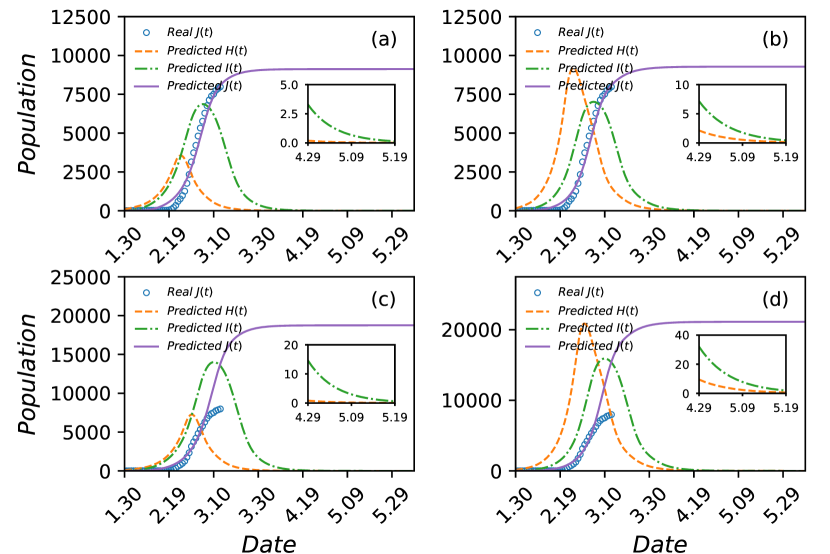
For South Korea, we use the reported data (?) of the number of confirmed cases between January 30 and March 13. The epidemic emerged mainly in the cities of Daegu and Gyeongsangbuk-do, so we set millions (the approximately combined population of the two cities). The two cities, being the epicenter, were locked down on February 21, so we have . The value of is not available, so we test two different values: 0.1 and 0.5, with the values of the other three model parameters estimated to be and , respectively. The prediction results for the two sets of parameter values are shown in Figs. 3(a) and 3(b), respectively. In spite of the difference in the choice of the value of parameter , in both cases our model predicts the following: occurrence of the epidemic peak (inflection point) on March 57, the final number of confirmed cases of about 9200, and the epidemic duration of approximately three months. These predictions agree with the current data in South Korea. For the two choices and , there is a small difference in the predicted ending date of the epidemic: about May 6 for the former and May 13 for the latter. We also simulate the hypothetical scenario where the lockdown of the two cities were delayed for five days, with the results for and shown in Figs. 3(c) and 3(d), respectively. Inevitably, the predicted curves of the accumulative number of confirmed cases deviate from the data, but the final epidemic size would double and the epidemic could last longer.
Prediction for Italy: Why is the mortality so high?
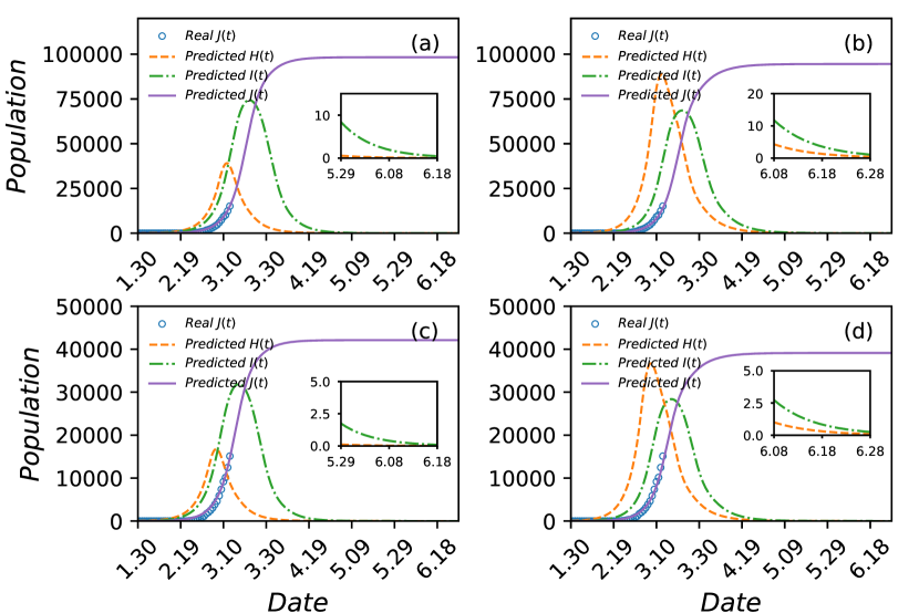
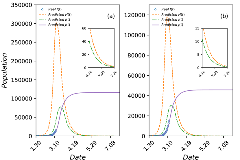
For Italy, we use the reported number of confirmed cases between January 30 and March 13. The entire country was locked down on March 8, so we have . The total population of Italy is millions. Figures 4(a) and 4(b) present the model prediction results of , , and , together with the actual up-to-date data, for and , respectively. There is a good agreement between the predicted and true behaviors of . Figures 4(c) and 4(d) display the prediction results corresponding to the parameter settings in Figs. 4(a) and 4(b), respectively, under the hypothetical scenario that the country were locked down five days earlier. It can be seen that the effect of an earlier lockdown would reduce the final epidemic size approximately by a factor of two.
There is a key difference between the lockdown of Wuhan in China and that of Italy. Especially, in China, confirmed individuals are treated at hospitals but in Italy, of such individuals are isolated in their home (undocumented) and only are treated, leading to a relatively large value of . The predicted results in Figs. 4(a) and 4(b), where the value of is relatively small, thus may not reflect the actual epidemic behavior. To remedy this deficiency, we carry out prediction for , with results shown in Fig. 5(a). It can be seen that the predicted curve still agrees with the actual data, but the predicted epidemic size now stands at about 75,000 and the predicted peak H-state population is an astounding 300,000. Simulation reveals that there will still be hundreds infected and hidden individuals after June 8. Our model predicts that, for Italy, for the more realistic case of , the epidemic will end at the beginning of August (around August 3), which is about 50 days later than that for the case of . A striking feature is that, toward the end of the epidemic, there are more H-state than I-state individuals, posing a significant challenge to control and prevention. The prediction that the H-state population can last longer than the I-state population is particularly worrisome, because it implies a higher likelihood of a future outbreak. Figure 5(b) shows the result for the hypothetical scenario of a five-day earlier lockdown, where both the peak I-state and H-state populations are more than halved, and the numbers of the two remaining populations would be less than 200 by May 19.
A puzzling phenomenon that has been widely noticed and discussed is the markedly higher mortality in Italy than that in South Korea, both being developed countries at the similar level. (As of March 18, the mortality among those infected is in Italy but it is only in South Korea.) Our model prediction for large values of provides a reasonable explanation. In particular, while the predicted number of confirmed cases does not depend strongly on the value of , the case of , which more closely describes the current effects of government actions in Italy, has devastating consequences. Especially, means that about of the virus-carrying individuals eventually enter into the R state after a time delay , without going through any medical treatment. Since the population in the R state consists of both recovered individuals and deaths, under the assumption that the death rate with COVID-19 is invariant across different countries, the significantly large fraction of people switching directly from the H state to the R state means significantly more deaths.
Prediction for Iran
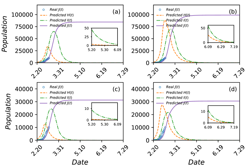
For Iran, lockdown occurs on March 7, so we have . The total population is millions. Model predicted results are shown in Figs. 6(a) and 6(b) for and , respectively. In both cases, the infected population will reach its peak around March 23. As for other countries, the value of does not affect the prediction of the inflection point. It can also be seen that, for a larger value of [Fig. 6(b)], the number of confirmed individuals is greater than that for the case in Fig. 6(a), and the duration is longer: for the former the epidemic is predicted to end on about July 21 while it is June 17 for the latter. Figures 6(c) and 6(d) present the respective model predicted results for and under the hypothetical scenario of imposing lockdown five days earlier, where the epidemic size could be significantly smaller with a much shorter duration.
Prediction of epidemic scenarios for United Kingdom
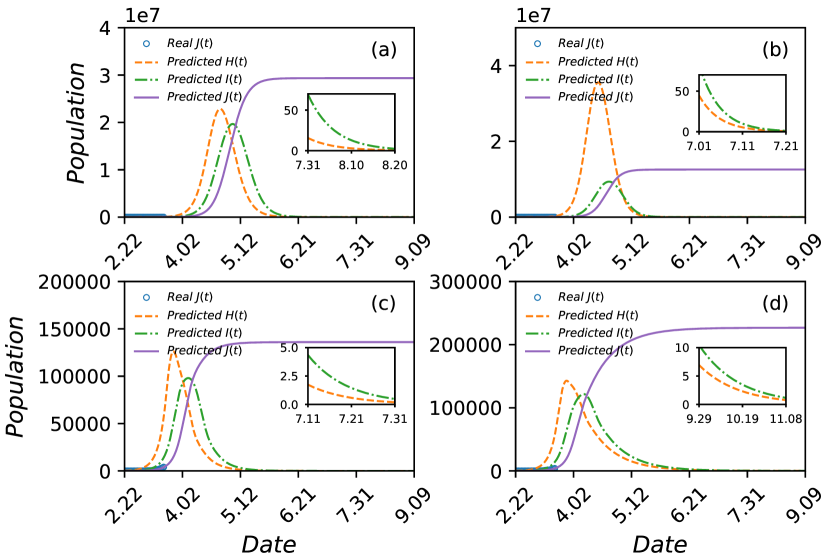
For United Kingdom, sparse data became available on February 1 with a few imported cases of infection, but the data after February 22 are more systematic. Model parameter optimization reveals that choosing February 1 or February 22 as the starting date of epidemic would lead to a different value of , but the value of is hardly affected: in both cases we have . The total population of the country is millions. We simulate four scenarios.
-
1.
Moderate fraction of undocumented cases () and absence of government imposed travel and social distancing restrictions. The model predicted results are shown in Fig. 7(a): of the population will be infected with approximately 30 million confirmed cases. The inflection point will occur around May 15 and the epidemic will be over on about August 20.
-
2.
High fraction of undocumented cases () and absence of government restrictions. The results are shown in Fig. 7(b): of the population will be infected with approximately 10 million confirmed cases. The inflection point will occur around April 25 and the epidemic will be over on about July 20.
-
3.
Moderate fraction of undocumented cases () and strict government imposed restrictions at a level similar to that of China: (the same value in China for ). The results are shown in Fig. 7(c): approximately confirmed cases, occurrence of inflection on about April 3, and end of epidemic at the end of July or beginning of August.
-
4.
Moderate fraction of undocumented cases () but with less strict government imposed restrictions: . As shown in Fig. 7(d), in this case, the eventual number of confirmed cases will be about , the inflection will occur on about April 7, and the epidemic will stretch into the beginning of November before it is over.
Based on the available data at the time of writing, the last scenario appears to fit with the situation in United Kingdom.
Discussion
We have developed a realistic, five-state epidemic spreading model with time delays for COVID-19, taking into account virulence of individuals in incubation, the non-Markovian characteristics associated with the various state transitions, and the exponential decay of population activity level under strict government actions. Our model requires four parameters to simulate the spreading dynamics: the fraction of undocumented virus-carrying individuals spontaneously recovered or died, the effective infection rate, the initial size of the population in incubation, and the rate of reduction in human activities due to government actions. These parameters can be obtained from government reports, reasoned, or estimated through a mathematical inverse optimization approach. The model is capable of real-time prediction, and has been validated as its prediction of the number of daily accumulative confirmed cases agrees remarkably well with the current data. The effects of government actions, as measured by the parameter , can vary greatly among different countries. For example, in South Korea, almost all possible individuals exposed to the virus went through nucleic-acid tests, while such tests are not being conducted in countries such as Japan, the United States, and United Kingdom, leading to abnormally low number of confirmed cases. Countries such as Italy are perhaps somewhere in between, so a large fraction of asymptomatic/undetected virus-carrying individuals without going through any medical treatment exists. In this case, the epidemic size would be significantly larger with a prolonged duration. This not only has provided a natural explanation for the abnormally high mortality in Italy, but also implied a devastating picture for the epidemic trend: even after the epidemic has been deemed over, there can still be a small population of asymptomatic individuals in the society, making a future outbreak and COVID-19 evolving into a long epidemic or a community disease a real possibility.
Our predicted scenarios for United Kingdom indicate that the epidemic would be catastrophic without government imposed travel and social distancing restrictions. The current restrictions would lead to about 220,000 confirmed cases and a prolonged epidemic duration into November. This prediction is consistent with that by the Imperial College COVID-19 Response Team (?). The best scenario leading to the least damage is when the government imposed restrictions as strict as those in China.
COVID-19 is unusual because even individuals in incubation can be highly infectious yet they themselves can be asymptomatic. The existence of even a small fraction of such individuals with an arbitrarily long incubation time in the population (H-state individuals), can be extremely worrisome, as they carry the virus and are capable of spreading it to the general public yet they appear healthy in every reasonable way and thus may never be identified without dramatic government actions. Right from the beginning of the COVID-19 pandemic, there was a concern that it could evolve into a community disease and will always be with us. However, this was merely a speculation without any quantitative justification. Our work has provided theoretical and modeling based evidence for the likelihood of COVID-19 becoming a community disease. This has grave consequences and significant implications. For example, for the current COVID-19 epidemic in China, our model predicts a few dozen such H-state individuals. As the government measures are gradually withdrawn, these individuals could diffuse into the general population, leading to the next COVID-19 epidemic/pandemic. But the currently implemented and enforced epidemic control policies cannot be maintained indefinitely for economical, social and other reasons. What should the government do then? Before the successful development of an effective and feasible vaccine, one possibility is to conduct universal testing of the entire population to identify the remaining H-state individuals. Having said that, we are not in a position to provide a solution to this problem. Rather, our goal was to generate scientific support for government policies on controlling and preventing future large scale COVID-19 epidemic, which we believe has been achieved in the current work.
Our model takes into account the effects of government imposed control and preventive measures and has been demonstrated to have the predictive power for the epidemic trend. The discovery of the sustained existence of a group of individuals in the hidden state provides the base for future policy making. Because of the vast difference among different countries and even among different regions in the same country in terms of factors such as medical facilities and the effectiveness of the government actions, it is necessary to carry out a more detailed analysis of the probability distributions of the time delays associated with the relevant state transitions, and to investigate how the changes in the distributions affect the inflection point, epidemic size and duration. In China, there is now evidence that many cases of mutual spreading occur in closed environments such as families, factories, and even prisons, which are not affected by travel restriction. The effects of such spreading scenarios on the epidemic need to be studied. Another issue is to investigate COVID-19 spreading dynamics on larger spatial scales. In particular, our model is especially suited for an isolated city such as Wuhan, where the current description and understanding of the spreading dynamics subject to rigorous implementation of government measures are reasonable. However, as the range of epidemic increases, the effect of large scale population movements on the spreading dynamics must be studied, possibly through the approach of network modeling with subpopulation dynamics. As the epidemic spreading begins to weaken or diminish, government actions will inevitably be relaxed. How to effectively prevent a second epidemic is an urgent problem. Also, is it possible to articulate time-dependent control and preventive measures that are adaptive to the development of the epidemic? And how to minimize the extent of control and travel restriction without sacrificing the expectations is another issue worth immediate attention.
Data Availability
All relevant data are available from the authors upon request.
Code Availability
All relevant computer codes are available from the authors upon request.
Acknowledgments
This work was supported by the National Natural Science Foundation of China (Grant Nos. 11975099, 11575041, 11675056 and 11835003), the Natural Science Foundation of Shanghai (Grant No. 18ZR1412200), and the Science and Technology Commission of Shanghai Municipality (Grant No. 14DZ2260800). YCL would like to acknowledge support from the Vannevar Bush Faculty Fellowship program sponsored by the Basic Research Office of the Assistant Secretary of Defense for Research and Engineering and funded by the Office of Naval Research through Grant No. N00014-16-1-2828.
Author Contributions
Y.-S.L., M.T. and Y.-C.L. designed research; Y.-S.L., Z.-M.Z., L.-L.H, J.K., and Z.-H.L. performed research; Y.-L.L., Z.-H.L., L.Z., D.-Y.W., and C.-Q.H. contributed analytic tools; Y.-S.L., Z.-M.Z., M.T., Z.L., and Y.-C.L. analyzed data; M.T., Z.L., and Y.-C.L. wrote the paper.
Competing Interests
The authors declare no competing interests.
Correspondence
To whom correspondence should be addressed. E-mail: tangminghan007@gmail.com; Ying-Cheng.Lai@asu.edu
References
- 1. National Health Commission of the People’s Republic of China (2020). Accessed March 2,2020.
- 2. Q. Li, et al., New Eng. J. Med. (2020).
- 3. C. P. E. R. E. Novel, et al., Zhong Hua Liu Xing Bing Xue Za Zhi 41, 145 (2020).
- 4. W.-J. Guan, et al., New Eng. J. Med. (2020).
- 5. C. Wang, P. W. Horby, F. G. Hayden, G. F. Gao, Lancet 395, 470 (2020).
- 6. Y. Zhou, Z. Ma, F. Brauer, Mathematical and Computer Modelling 40, 1491 (2004).
- 7. G. Chowell, S. Blumberg, L. Simonsen, M. A. Miller, C. Viboud, Epidemics 9, 40 (2014).
- 8. W. E. R. Tea, New England Journal of Medicine 371, 1481 (2014).
- 9. S. Towers, et al., Epidemics 17, 50 (2016).
- 10. J. T. Wu, K. Leung, G. M. Leung, Lancet 395, 689 (2020).
- 11. T. Zhou, et al., Journal of Evidence-Based Medicine (2020).
- 12. X. Xiao-ke, et al., µç×ӿƼ¼´óѧѧ±¨ 49, 1 (2020).
- 13. Z. Yang, et al., Journal of Thoracic Disease (2020).
- 14. Y. Yue, et al., Scientia Sinica Mathematica (2020).
- 15. M. Chinazzi, et al., Science (2020).
- 16. R. Li, et al., Science (2020).
- 17. Z. Du, et al., medRxiv (2020).
- 18. K. Levenberg, Quarterly of applied mathematics 2, 164 (1944).
- 19. D. W. Marquardt, Journal of the society for Industrial and Applied Mathematics 11, 431 (1963).
- 20. B. Kaltenbacher, A. Neubauer, O. Scherzer, Iterative Regularization Methods for Nonlinear Ill-Posed Problems, vol. 6 (Walter de Gruyter, 2008).
- 21. World Health Organization (2020). Accessed March 13, 2020.
- 22. N. M. Ferguson, et al., Impact of non-pharmaceutical interventions (NPIs) to reduce COVID- 19 mortality and healthcare demand (2020). Report of Imperial College COVID-19 Response Team, March 16,2020.