Geometric Sparsification of Closeness Relations:
Eigenvalue Clustering for Computing Matrix Functions

Abstract

We show how to efficiently solve a clustering problem that arises in a method to evaluate functions of matrices. The problem requires finding the connected components of a graph whose vertices are eigenvalues of a real or complex matrix and whose edges are pairs of eigenvalues that are at most $\delta$ away from each other. Davies and Higham proposed solving this problem by enumerating the edges of the graph, which requires at least $\Omega(n^{2})$ work. We show that the problem can be solved by computing the Delaunay triangulation of the eigenvalues, removing from it long edges, and computing the connected components of the remaining edges in the triangulation. This leads to an $O(n\log n)$ algorithm. We have implemented both algorithms using CGAL, a mature and sophisticated computational-geometry software library, and we demonstrate that the new algorithm is much faster in practice than the naive algorithm. We also present a tight analysis of the naive algorithm, showing that it performs $\Theta(n^{2})$ work, and correct a misrepresentation in the original statement of the problem. To the best of our knowledge, this is the first application of computational geometry to solve a real-world problem in numerical linear algebra.

1 Introduction

This paper proposes and analyzes efficient algorithms to sparsify transitive closeness relations of points in the Euclidean plane. The problem that we solve is an important step in a general method to efficiently compute functions of matrices.

More specifically, given a set $\Lambda$ of $n$ points in the plane (real or complex eigenvalues of a matrix, in the underlying problem), we wish to compute the connected components of a graph $G(\Lambda,\delta)$ whose vertices are the $n$ points and whose edges connect pairs of points that are within distance at most $\delta$ of each other, for some real $\delta>0$. Points that are at most $\delta$ apart are said to be close, and in this problem closeness is transitive. The connected components of $G(\Lambda,\delta)$ partition $\Lambda$ into disjoint minimal well-separated clusters. That is, points in two different clusters are more than $\delta$ apart, and the clusters cannot be reduced while maintaining this property.

This problem is an important step in a method proposed by Davies and Higham [8][12, Chapter 9] to compute a function $f(A)$ of a square real or complex matrix $A$. We describe the overall method and the role of the eigenvalue-clustering problem in it in Section 2. Here it suffices to say that the eigenvalue-clustering problem allows the use of a divide an conquer strategy while reducing the likelihood of numerical instability. Nearby eigenvalues in separate clusters create an instability risk; this is why we want the clusters to be well separated. Large clusters reduce the effectiveness of the divide and conquer strategy, which is why clusters should be as small as possible.

Solving the problem in $O(n^{2}\alpha(n))$ time, where $\alpha$ is the inverse Ackermann function, is easy. We start with minimal but illegal singleton clusters, and then test each of the $n(n+1)/n=O(n^{2})$ eigenvalues pairs for closeness. If they are close and in different clusters, we merge their two clusters. The overall time bound assumes that the data structure that represents the disjoint sets supports membership queries and merge operations in $O(\alpha(n))$ time each, amortized over the entire algorithm [7, Chapter 21].

The main contributions of this paper are two algorithms that solve this problem in $O(n\log n)$ time. One, presented in Section 4, is very simple but is only applicable when all the eigenvalues are real (all the points lie on the real axis). The other algorithm, which is applicable to any set of points in the plane, is also fairly simple, but uses a sophisticated building block from computational geometry, namely the Delaunay triangulation. We present this algorithm in Section 5.3. The Delaunay triangulation is also a graph whose vertices are $\Lambda$, but it is planar and therefore sparse, having only $O(n)$ edges. It turns out that when edges longer than $\delta$ are removed from a Delaunay triangulation of $\Lambda$, the remaining graph has exactly the same connected components as $G(\Lambda,\delta)$. The Delaunay triangulation can be constructed in $O(n\log n)$ time, giving as an effective sparsification mechanism for $G(\Lambda,\delta)$. The algorithm for the real case also constructs a Delaunay triangulation, but in this case the triangulation is particularly simple.

Algorithms in computational geometry, like the algorithms that construct the Delaunay triangulation, can suffer catastrophic failures when implemented using floating-point arithmetic. Therefore, we implemented our algorithms using CGAL, a computational-geometry software library that supports both floating-point arithmetic and several types of exact arithmetic systems. This implementation is described in detail in Section 6.

Experimental results, presented in Section 7, demonstrate that the new algorithms outperform the naive algorithm by large margins. The results also demonstrate that the extra cost of exact arithmetic is usually insignificant, at least when using an arithmetic system that does use floating-point arithmetic whenever possible.

Our paper contains two additional contributions. The first, presented in Section 5.2, is an amortized analysis of the naive algorithm coupled with a particularly simple data structure to represent disjoint sets. The analysis shows that even with this simple data structure, proposed by Davies and Higham (and used many times in the literature in various variants), the total running time of the naive algorithm is only $O(n^{2})$.

The second is an observation, presented in Appendix A, that an alternative definition of the required eigenvalue partition, proposed by Davies and Higham is not equivalent to the connected components of $G(\Lambda,\delta)$ and is not particularly useful in the overall method for evaluating $f(A)$.

Let’s get started.

2 Background

Figure 1: The overall structure of the Davies-Higham method for computing a function $f(A)$ of a matrix $A$.

A scalar function $f\colon\mathbb{C}\rightarrow\mathbb{C}$ can be extended to square real and complex matrices by letting $f$ act on the eigenvalues of the matrix. That is, if $A\in\mathbb{C}^{n\times n}$ is diagonalizable so $A=VDV^{-1}$ with $D$ diagonal, then $f(A)=Vf(D)V^{-1}$ has the same eigenvectors as $A$ but eigenvalues that have been transformed by $f$; here $f(D)$ denotes a diagonal matrix with diagonal entries $(f(D)_{ii}=f(D_{ii})$. The definition can be extended to non-diagonalizable matrices in one of several equivalent ways [12]. Functions of matrices have many applications [12].

For many functions $f$ of practical importance, such as the square root and exponentiation ($f(x)=e^{x})$, there are specialized algorithms to compute $f(A)$. There are also several general techniques to evaluate $f(A)$. Among them is a sophisticated and efficient method due to Davies and Higham [8][12, Chapter 9]. The problem that we solve in this paper is a subroutine the Davies-Higham method.

The Davies-Higham method can be viewed in two ways. One is as a generalization and adaptation of an older method due to Parlett [17][12, Section 4.6]. The so-called Schur-Parlett method computes the Schur decomposition $A=Q_{S}TQ_{S}^{*}$, where $T$ is triangular and $Q_{s}$ is unitary, evaluates $f(T)$ using a simple recurrence, and forms $f(A)=Q_{S}f(T)Q_{S}^{*}$. This method is applicable to any function $f$, but it fails when $A$ has repeated or highly clustered eigenvalues. When it does work, this method evaluates $f(A)$ in $\Theta(n^{3})$ time. In particular, all three steps of the method take cubic time time: the Schur decomposition, the evaluation of $f(T)$, and the matrix multiplications required to form $f(A)$ (the latter step can be asymptotically faster if one uses fast matrix multiplication). The Davies-Higham method, which is illustrated in Figure 1, partitions the eigenvalues into well-separated clusters, reorders the Schur decomposition $T=Q_{R}T_{R}Q_{R}^{*}$ so that clusters are contiguous along the diagonal of $T_{R}$, applies some other algorithm to evaluate $f$ on diagonal blocks of $T_{R}$, and then applies a block version of Parlett’s recurrence to compute the off-diagonal blocks of $T_{R}$. The partitioning of the spectrum $\Lambda$ of $A$ into well-separated cluster is designed so that the solution of the recurrence equations for the off-diagonal blocks is numerically stable.

The other way to view the Davies-Higham is as a divide-and-conquer algorithm. The technique that must be applied to evaluate $f$ on diagonal blocks of $T_{R}$ have super-cubic cost. The technique that Davies and Higham proposed is a Pade approximation of $f$, and its cost is approximately quartic in the dimension of the block. Therefore, it is best to apply this technique to diagonal blocks that are as small as possible, to attain a total cost that is as close as possible to cubic, not quartic. That is, the Davies-Higham chops the original problem into sub-problems that are as small as possible (the diagonal blocks of $T_{R}$), solves each one using an expensive algorithm, and then merges the solutions. The splitting and merging phases are cubic.

Let us now review the entire Davies-Higham method, as illustrated in Figure 1. We start by computing the Schur decomposition $A=Q_{S}TQ_{S}^{*}$. If $A$ is real with complex eigenvalues, we compute the so-called real Schur decomposition. In this case, complex eigenvalues form conjugate pairs that are represented as $2$-by-$2$ diagonal blocks in $T$ (so $T$ is not triangular but block triangular with $1$-by-$1$ and $2$-by-$2$ blocks). Next, we partition the eigenvalues into clusters using a simple clustering rules described below in Section 3. This clustering algorithm is the main focus of this paper. In Figure 1, the clusters are represented by coloring the eigenvalues, which lie along the diagonal of $T$. Now we need to reorder the eigenvalues so that clusters are contiguous while maintaining the triangular structure and while maintaining the reordered matrix $T_{R}$ as a Schur factor of $A$. That is, we transform $T$ into $T_{R}$ using unitary similarity. The reordering also costs $O(n^{3})$ time [2, 14]. Now we evaluate $f$ on diagonal blocks of $T_{R}$ and then solve Sylvester equations for the off-diagonal blocks of $f(T_{R})$. The separation between clusters of eigenvalues is designed to minimize errors in the solution of these equations. We note that the clustering criterion proposed by Davies and Higham does not guarantee small errors; it serves as a proxy for a criterion that is too difficult to use.

When $A$ is a real matrix with complex eigenvalues, complex eigenvalues form conjugate pairs and the two eigenvalues in each pair are kept together in the reordering, in order to maintain the block-diagonal structure of the Schur factor. We handle this case by including only one eigenvalue from each pair in the input to the partitioning problem, the one with positive imaginary part. Its conjugate is then placed in the same cluster.

3 The Spectrum-Partitioning Criterion

Davies and Higham define the criteria for the partitionining of the eigenvalues in two different ways. We present first the definition that is both algorithmically useful and correct in the sense that it serves the overall algorithm well.

Definition 1.

The $\delta$-closeness graph $G(\Lambda,\delta)$ of a set of complex numbers $\Lambda=\{\lambda_{1},\lambda_{2},\ldots,\lambda_{n}\}$ (possibly with repetitions) is the graph whose vertex set is $\Lambda$ and whose edge set consists of all the pairs $\{\lambda_{i},\lambda_{j}\}$ for which $|\lambda_{i}-\lambda_{j}|\leq\delta$.

We denote the connected components of $G=G(\Lambda,\delta)$ by $C_{1}^{(G)},\ldots,C_{k}^{(G)}$, and when the graph is clear from the context, we denote the components by $C_{1},\ldots,C_{k}$. We view connected components as sets of vertices, so $C_{1},\ldots,C_{k}$ are disjoint sets of eigenvalues. We denote the connected component in $G$ that contains $\lambda_{i}$ by $C^{(G)}(\lambda_{i})$ and by $C(\lambda_{i})$ if the graph is clear from the context.

Partitioning $\Lambda$ by connected components in $G(\Lambda,\delta)$ is effective in the Davies-Higham algorithm. This partitioning reduces (in a heuristic sense explained in their paper) the risk of instability while admitting efficient partitioning algorithms, including one proposed in the Davies and Higham paper. We note that Davies and Higham imply that the connected components of $G(\Lambda,\delta)$ are equivalent to the a partition that satisfies two specific conditions, but this is not the case, as we show in Appendix A.

4 An Algorithm for Real Eigenvalues

Davies and Higham proposed a partitioning algorithm that works for both real and complex eigenvalues, but we start with a new algorithm that is specialized for the real case and is both simpler and more efficient than the Davies-Higham algorithm. We sort the eigenvalues so that $\lambda_{\pi(1)}\leq\lambda_{\pi(2)}\leq\cdots\leq\lambda_{\pi(n)}$ ($\pi$ is a permutation that sorts the eigenvalues). We then create an integer vector $g$ of size $n$ and assign

$$g_{i}=\begin{cases}1&|\lambda_{\pi(i)}-\lambda_{\pi(i-1)}|>\delta\\ 0&|\lambda_{\pi(i)}-\lambda_{\pi(i-1)}|\leq\delta\;,\end{cases}$$

denoting $\lambda_{\pi(0)}=-\infty$ so that $g_{1}$ is always $1$. The vector $g$ marks gaps in the spectrum (the set of eigenvalues). We now compute the prefix sums of $g$,

$$c_{i}=\sum_{j=1}^{i}g_{i}\;.$$

Now $c_{i}$ is the label (index) of the cluster that eigenvalue $\lambda_{\pi(i)}$ belongs to.

The running time of this technique is $\Theta(n\log n)$ assuming that we use a comparison-based sorting algorithm.

We defer the correctness proof for this algorithm to the next section, because the proof is a special case of a more general analysis for the complex case, but we state the result here.

Theorem 2.

Partitioning $\Lambda\subset\mathbb{R}$ by sorting the eigenvalues and splitting whenever two adjacent eigenvalues are more than $\delta$ away creates a partition that is identical to the connected components of $G(\Lambda,\delta)$.

5 An Algorithm for Complex Eigenvalues

If $A$ has complex eigenvalues, the simple method of Section 4 no longer works. Later in this section we present a very efficient algorithm to partition complex eigenvalues, but we start with a simpler variant that is closer to the algorithm proposed by Davies and Higham.

5.1 The Davies-Higham Partitioning Algorithm.

Davies and Higham propose a partitioning algorithm that works for both real and complex eigenvalues, but their paper (and Higham’s book) do not prove that it is correct, does not specify exactly how clusters are represented, and does not analyze the complexity of the algorithm.

Their algorithm is incremental. It maintains a partitioning of a subset of the eigenvalues. When step $t$ ends, the partitioning is valid for the subgraph that contain all the vertices (eigenvalues) and all the edges $\{\lambda_{i},\lambda_{j}\}$ for which $i\leq t$ or $j\leq t$. Initially, every eigenvalue forms a singleton cluster, because we have not considered any edges (closeness relations) yet. (The text of Davies and Higham imples that the singleton cluster for $\lambda_{i}$ is formed only in the beginning of step $i$ and only if $\lambda_{i}$ is not already part of a larger cluster, but this only makes the algorithm a little harder to understand.)

In step $i$, the algorithm computes the distances $|\lambda_{i}-\lambda_{j}|$ for all $j>i$ such that $\lambda_{j}$ is not already in the same cluster as $\lambda_{i}$. If the distance is smaller than $\delta$, meaning that a new edge has been discovered in the graph, the clusters that contain $\lambda_{i}$ and $\lambda_{j}$ are merged.

Davies and Higham do not spell out exactly how clusters are represented, but their text implies that they record in a vector $c$ the label of the cluster of every eigenvalue; that is, $c_{i}$ is the label (integer) of the cluster that contains $\lambda_{i}$. When they merge clusters with indices $x$ and $y>x$, they relabel eigenvalues in $y$ as belonging to $x$, and they decrease by $1$ every label higher than $y$. The relabeling of clusters higher than $y$ may simplify later phases in the overall algorithms, because at the end of the algorithm the clusters are labeled contiguously $1,\ldots,k$, but it is clearly also possible to relabel the clusters once at the end in $\Theta(n)$ operations.

Davies and Higham do not prove the correctness of this algorithm (but this is fairly trivial) and they do not analyze its complexity. The loop structure of their algorithm shows that its running time is $\Omega(n^{2})$ and $O(n^{3})$ but the exact asymptotic complexity is not analyzed.

5.2 Disjoint-Sets Data Structures for Connected Components

The Davies-Higham partitioning algorithm is an instantiation of a generic method to compute connected components. The generic method maintains a disjoint-sets data structure, initialized to a singleton for every vertex. The edges of the graph are scanned, in any order. For each edge $\{i,j\}$, the method determines the sets $S_{i}$ and $S_{j}$ that $i$ and $j$ belong to, respectively, and if $S_{i}\neq S_{j}$, the two sets are merged. The correctness of the Davies-Higham algorithm is a consequence of the correctness of this general method.

There are many ways to represent the sets and to perform the operations that find $S_{i}$ given $i$ (the so-called find operation) and merge $S_{i}$ and $S_{j}$ (the so-called union operation). The most efficient general-purpose data structure uses rooted trees to represent the sets and optimizations called union by rank and path compression to speed up the operations; this data structure and algorithms guarantee an $O(m\alpha(n))$ complexity for a sequence of $m$ union or find operations on a set of $n$ elements (in all the subsets combined), where $\alpha$ is the inverse Ackermann function, whose value for any practical value of $n$ is at most $4$. The Davies-Higham algorithm performs $n(n-1)/2=\Theta(n^{2})$ find operations and at most $n-1$ union operations (since every union operation reduces the number of subsets by $1$), so the complexity with this data structure is $O(n^{2}\alpha(n))$.

However, in our case even the simpler data structure and algorithms that Davies and Higham proposed guarantee an $O(n^{2})$ complexity. The number of union operations at most $n-1$, so even if every union operation costs $\Theta(n)$ to scan the vector $c$ and to relabel some of the components, the total cost of the union operations is still $O(n^{2})$. The find operations cost $O(1)$, so their total cost is again $O(n^{2})$.

5.3 An Efficient Geometric Partitioning Algorithm

The $\delta$-closeness graph can have $n(n-1)/2=\Theta(n^{2})$ edges so constructing the graph requires $\Theta(n^{2})$ operations. The large number of edges also implies that the total cost of the disjoint-set operations is high, $\Omega(n^{2})$.

We have discovered that a sparse graph with only $O(n)$ edges and that can be constructed in $O(n\log n)$ operations has exactly the same connected components. This graph is the well-known Delaunay triangulation of the spectrum $\Lambda$, when viewed as a set of points in the plane. We begin with definitions of the Delaunay triangulation and of related geometric objects, specialized to the Euclidean plane, as well with a statement of key properties of them and key relationships between them. For further details on these objects, see [9, 11].

Definition 3.

Given a set of points $\Lambda=\{\lambda_{1},\lambda_{2},\ldots,\lambda_{n}\}$ in the plane, the Voronoi cell of $\lambda_{i}$ is the set of all points that are closer to $\lambda_{i}$ than to any other point in $\Lambda$. A Voronoi edge is a nonempty set of points that are equidistant from $\lambda_{i}$ and $\lambda_{j}\neq\lambda_{i}$ and closer to $\lambda_{i}$ and $\lambda_{j}$ than to any other point in $\lambda$. A Voronoi vertex is a point that is closest to three or more points in $\Lambda$. The Voronoi diagram of $\Lambda$ is the ensemble of Voronoi faces, edges, and vertices.

Definition 4.

The Delaunay Graph of a set of points $\Lambda=\{\lambda_{1},\lambda_{2},\ldots,\lambda_{n}\}$ in the plane is the dual of their Voronoi diagram: $\{\lambda_{i},\lambda_{j}\}$ is an edge of the Delaunay graph if and only if the cells of $\lambda_{i}$ and $\lambda_{j}$ share an edge.

We note that if the Voronoi cells of $\lambda_{i}$ and $\lambda_{j}$ share a single point, then this point is a Voronoi vertex and not a Voronoi edge, and in such a case $\{\lambda_{i},\lambda_{j}\}$ is not an edge of the Delaunay graph. In many cases it is convenient to view an edge of the Delaunay graph not only as a pair of vertices (points in the plane), but also as a line segment, but for our application this is not important. The Delaunay triangulation is any completion of a Delaunay graph to a triangulation of the plane.

The efficiency and correctness of our algorithm depends on two key properties of the Delaunay graph.

Lemma 5.

[9, Theorem 9.5] Delaunay graphs and Delaunay triangulations are planar graphs.

Lemma 6.

[9, Theorem 9.6 part ii]$\{\lambda_{i},\lambda_{j}\}$ is an edge of the Delaunay graph if and only if there is a closed disk that contains $\lambda_{i}$ and $\lambda_{j}$ on its boundary and does not contain any other point of $\Lambda$.

We are now ready to state and prove our main result.

Figure 2: An illustration of the proof of Theorem 7. The eigenvalues $\lambda_{i}$ and $\lambda_{j}$ lie on a diameter of the gray disk. The illustration shows both $\lambda_{k}$ in the interior of the disk and $\lambda_{k^{\prime}}$ on its boundary. The length of the diameter is at most $\delta$ but the dashed segments are all strictly shorter than the diameter.

Theorem 7.

Let $\Lambda=\{\lambda_{1},\lambda_{2},\ldots,\lambda_{n}\}$ be a set of points in the plane, let $G(\Lambda,\delta)$ be the graph whose vertex set is $\Lambda$ and whose edge set contains all the pairs $\{\lambda_{i},\lambda_{j}\}$ for which the Euclidean distance between $\lambda_{i}$ and $\lambda_{j}$ is at most $\delta$, for some real $\delta>0$. Let $D(\Lambda)$ be the Delaunay graph of $\Lambda$ and let $D(\Lambda,\delta)$ the subset of the graph that contains only Delaunay edges with length at most $\delta$. We claim that $G(\Lambda,\delta)$ and $D(\Lambda,\delta)$ have identical connected components.

Proof.

Since the edge set of $D(\Lambda,\delta)$ is a subset of the edge set of $G(\Lambda,\delta)$, the connected components of $D(\Lambda,\delta)$ are subsets of the connected components of $G(\Lambda,\delta)$. That is, for every $\lambda_{i}$ we have $C^{(D)}(\lambda_{i})\subseteq C^{(G)}(\lambda_{i})$. It remains to show that $C^{(G)}(\lambda_{i})\subseteq C^{(D)}(\lambda_{i})$ also holds. We prove this claim by showing that for every edge $\{\lambda_{i},\lambda_{j}\}$ in $G(\Lambda,\delta)$ there is a path between $\lambda_{i}$ and $\lambda_{j}$ in $D(\Lambda,\delta)$.

Assume the contrary, namely, there is an edge $\{\lambda_{i},\lambda_{j}\}$ in $G(\Lambda,\delta)$ such that there is no path in $D(\Lambda,\delta)$ connecting the vertices $\lambda_{i}$ and $\lambda_{j}$. Of all such edges, let $\{\lambda_{i},\lambda_{j}\}$ be such that $|\lambda_{i}-\lambda_{j}|$ is the smallest (that is, the Euclidean distance between the eigenvalues is the shortest). In particular, $\lambda_{i}$ and $\lambda_{j}$ are not connected by an edge in the Delaunay graph, even though the distance between them is at most $\delta$ as the edge $\{\lambda_{i},\lambda_{j}\}$ appears in $G(\Lambda,\delta)$. Lemma 6 implies that every circle with $\lambda_{i}$ and $\lambda_{j}$ on its boundary contains a third point of $\Lambda$, in the interior or on its boundary. Consider the specific circle for which $\lambda_{i}$ and $\lambda_{j}$ lie on a diameter and let $\lambda_{k}\in\Lambda$ be a point inside that circle or on its boundary. As we have just observed, since $\lambda_{i}$ and $\lambda_{j}$ are endpoints of an edge in $G(\Lambda,\delta)$, the length $|\lambda_{i}-\lambda_{j}|$ is at most $\delta$. Then, both $|\lambda_{i}-\lambda_{k}|$ and $|\lambda_{k}-\lambda_{j}|$ are smaller than $\delta$. Now, we have two cases: (i) $\lambda_{i}$ and $\lambda_{k}$ are connected in $D(\Lambda,\delta)$, and $\lambda_{k}$ and $\lambda_{j}$ are connected in $D(\Lambda,\delta)$. But this forms a path in $D(\Lambda,\delta)$ between $\lambda_{i}$ and $\lambda_{j}$, which contradicts our assumption that such a path does not exist. (ii) One of the pairs in Case (i) is not connected in $D(\Lambda,\delta)$: then either $\lambda_{i}$ and $\lambda_{k}$ are not connected in $D(\Lambda,\delta)$, or $\lambda_{k}$ and $\lambda_{j}$are not connected in $D(\Lambda,\delta)$, or both are not connected. Obviously, both pairs are connected in $G(\Lambda,\delta)$ because the distances are shorter than $\delta$. However this contradicts the fact that $\lambda_{i}$ and $\lambda_{j}$ are the pair with this property having minimum distance between them. In either case we have a contradiction, which proves our assertion. ∎

We now prove Theorem 2.

Proof.

When all the eigenvalues are real, their Voronoi cells are infinite slabs separated by vertical lines that cross the real axis half way between adjacent eigenvalues. Therefore, all the edges of the Delaunay triangulation connect adjacent eigenvalues. Delaunay edges longer than $\lambda$ are prunned from $D(\Lambda,\delta)$, implying that the sort-and-split algorithm indeed forms the connected components of $D(\Lambda,\delta)$. ∎

Lemma 5 guarantees that the number of edges in the Delaunay graph is only $O(n)$. The Delaunay graph can be easily computed from the Voronoi diagram in $O(n)$ time, and the Voronoi diagram itself can be computed in $O(n\log n)$ time and $O(n)$ storage [9, Theorem 7.10]. There are also randomized algorithms that compute the Delaunay triangulation directly in $O(n\log n)$ expected time  [9, Theorem 9.12 and Section 9.6]. We can use algorithms that compute the Delaunay triangulation directly and not the Delaunay graph because every edge that is added to the graph to triangulate it and that remains after pruning long edges (its length is at most $\delta$) is also an edge of $G(\Lambda,\delta)$, so it does not modify the connected components that we compute.

6 Implementation

We have implemented two different algorithms for the complex case, one of them using two different arithmetic systems. All the algorithms were implemented in C++. We implemented the algorithm that constructs $G(\Lambda,\delta)$ explicitly and that computes its connected components using linked-lists to represent the disjoint-set data structure. The complexity of this implementation is $\Theta(n^{2})$. We also implemented an algorithm that computes the Delaunay triangulation, prunes edges longer than $\delta$ from it to form $D(\Lambda,\delta)$, and computes the connected components of $D(\Lambda,\delta)$. The computation of the Delaunay triangulation was done using the GAL library [3]. CGAL allows the use of several arithmetic systems; we tested the algorithm using three different ones, including two that are exact, as explained later.

We used exact arithmetic to run the Delaunay triangulation because computational-geometry algorithms can fail catastrophically when implemented in floating point arithmetic [13]. Briefly, this is caused because the algorithms compute many predicates of the input objects and of computed geometric objects and the use of floating-point arithmetic can easily lead to a set of binary outcomes of the predicates that are not consistent with any input. Arithmetic operations carried out on exact representations can be expensive and unlike floating-point arithmetic opeartions, do not necessarily run in constant time each. Therefore, the use of asymptotic operation counts, such as $\Theta(n\log n)$ operations, may not have much predictive value for actual running times. To address this, we report below on experiments that show that the Delaunay algorithm is faster than a naive algorithm that constructs all of $G(\Lambda,\delta)$, even when the latter is implemented in floating-point arithmetic.

More specifically, we ran the Delaunay-based algorithm using double-precision floating point arithmetic, using rational arithmetic, and using filtered rational arithmetic. The most informative results are those of the filtered arithmetic, which is exact but which resorts to the use of rational numbers only when the use of floating-point numbers cannot guarantee the correct evaluation of a predicate. This arithmetic system is usually almost as fast as floating-point arithmetic; it slows down only in difficult cases. The floating-point performance results are presented mostly in order to quantify the cost of exact arithmetic. The pure rational results are presented mostly to demonstrate the effectiveness of the filtered arithmetic system.

CGAL includes two implementations of algorithms that compute the 2-dimensional Delaunay triangulation[1, 5, 10]. One algorithm is an incremental algorithm that inserts points into the triangulation in a biased randomized order [1]. An insertion of a vertex with degree $d$ costs $\Theta(d)$. The expected running time of this algorithm is $O(n\log n)$, but the worst-case running time is $O(n^{2})$. When the set of points is not known in advance, a different algorithm that maintains a Delaunay hierarchy [10] often runs faster, but this is not the case in our application. We tested the Delaunay-hierarchy variant and it was indeed a bit slower. The asymptotic worst-case and expected running times of this algorithm are similar to (or worse, for some insertion orders) those of the random-insertion-order algorithm. Curiously, CGAL does not include a deterministic worst-case $O(n\log n)$ Delaunay-triangulation algorithm, even though such algorithms are older than the incremental algorithms [9, 11]; it appears that they are usually slower in practice than the expected-case $O(n\log n)$ algorithms.

The naive algorithms do not require an exact-arithmetic implementation, since distance computations in the plane are accurate (see [12, Sections 3.1 and 3.6]), which means that the computed edge set of $G(\Lambda,\delta)$ will include all the edges whose exact length is below $\delta-\epsilon$ and will exclude all the edges whose length is above $\delta+\epsilon$, both for some $\epsilon$ much smaller than $\delta$. We also use floating-point arithmetic to prune the Delaunay triangulation, for the same reason.

6.1 Parallelism

The algorithms that we propose can be parallelized, but by reducing the total work to $\Theta(n\log n)$, we essentially eliminate the need to parallelize this part of the Davies-Higham method.

The algorithm for the real case can be easily and effectively parallelized, because there are effective parallel algorithms for both sorting and parallel prefix [15]. The algorithm for the complex case requires a parallel two-dimensional Delaunay triangulation. Several such algorithms have been developed [4, 6, 16], but unfortunately, none of them have been implemented in CGAL or in any other robust library.

However, given that our algorithm are designed to be used in an $\Omega(n^{3})$ method whose critical path has length $\Omega(n)$ (the Schur decomposition), the $O(n\log n)$ cost of our algorithm is unlikely to create a significant Amdahl-type bottleneck even if it remains sequential.

7 Experimental Results

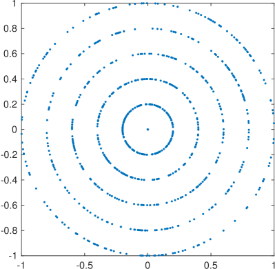
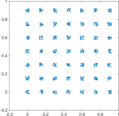
Figure 3: Examples of eigenvalue distributions that we used for testing. The plot on the left shows $999$ eigenvalues placed randomly on one of 5 circles that are spaced $0.2$ apart, as well as one eigenvalue at the origin. The eigenvalues are distributed evenly among the circles and the angular position of each eigenvalue is random with uniform distribution. The plot on the right shows $1000$ eigenvalues placed randomly and uniformly in one of several squares with a side of length $0.04$ and with centers spaced every $0.15$. Again, the eigenvalues are distributed among the squares evenly.

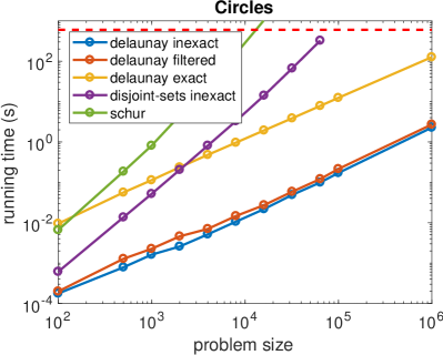
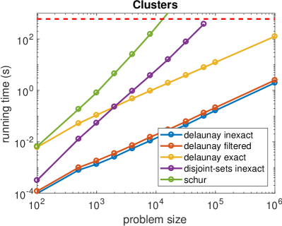
Figure 4: The running time of the algorithms on two different distributions of eigenvalues, as a function of the problem size $n$. The distribution used to produce the graph on the left is exactly the distribution shown on the left in Figure 3. The distribution used to produce the graph on the right is similar to the distribution shown on the right in Figure 3, but each cluster was distributed uniformly in a square with side length $0.02$. The running times did not change much when we modified the side of these squares to $0.15$ (so that the eigenvalues are distributed almost uniformly in the unit square) and to $2\times 10^{-10}$, a very tight clustering. We stopped very slow runs after 10 minutes; the dashed red line shows this limit.

We conducted experiments to assess the running times of the algorithms. We compiled the codes using the Microsoft C++ compiler version 19 using the O2 optimization level and we used version 4.13 of GCAL. We also include, for reference, the running times of the $\Theta(n^{3})$ Schur decomposition in Python’s scipy.linalg package, which uses LAPACK and an optimized version of the BLAS to compute the decomposition. This decomposition is the first step in the Davies-Higham method.

We ran all the experiments on a computer with a quad-core 3.5 GHz i5-4690K processor and 16 GB of 800 MHz DDR3 DRAM running Windows 10. Our codes are single threaded, so they used only one core. The Schur-decomposition runs used all the cores.

We evaluated the algorithms using two different distributions of eigenvalues, illustrated in Figure 3. One distribution includes an eigenvalue at the origin and the rest are placed on concentric circles with radii that differ by more than $\delta$, so that no cluster spans more than one circle. Each circle contains approximately the same number of eigenvalues and the location of each eigenvalue on its circle is random and uniform. More specifically, we used $\delta=0.1$, as recommended by Davies and Higham, and radii separation of $0.2$. The other distribution splits the eigenvalues evenly among squares whose centers are more than $\delta$ apart. The eigenvalues in each square are distributed uniformly in the square. We tested this distribution with $\delta=0.1$ and squares whose centers are $0.15$ apart, and with sides of $2\times 10^{-10}$, $0.02$, or $0.15$. In the first two cases (sides of $2\times 10^{-10}$ and $0.02$) the eigenvalues in each square form a single cluster, separate from those of other squares. When the squares have sides of length $0.15$, clusters often span more than one square (the eigenvalues are distributed approximately uniformly in the unit square).

The results show that the Delaunay-based algorithm are much faster than the naive algorithm. The different slopes on the log-log scale indicate that the algorithms run in approximately polynomial times but with different polynomial degrees. The results also show that the overhead of exact arithmetic, when using the filtered implementation, is minor. The overhead of naive rational arithmetic is considerable; it is more than 60 times slower than floating-point arithmetic and about 50 times slower than the filtered rational arithmetic.

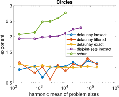
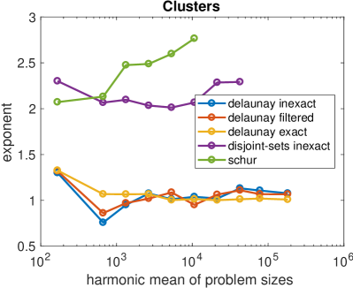
Figure 5: Estimates of the polynomial degree of the running times. For each pair of successive problem sizes $n_{1}$ and $n_{1}$ that resulted in running times of $T(n_{1})$ and $T(n_{2})$ using a particular algorithm, these graphs plot $\log(T(n_{2})/T(n_{2}))/\log(n_{2}/n_{1})$ against the harmonic mean of $n_{1}$and $n_{2}$.

Figure 5 estimates the degree of the polynomial running times. For each algorithm and for each pair of running times $T(n_{1})$ and $T(n_{2})$ on problems of sizes $n_{1}$ and $n_{1}$, the graphs show

$$\frac{\log\left(T(n_{2})/T(n_{2})\right)}{\log\left(n_{2}/n_{1}\right)}$$

as a function of the harmonic mean of $n_{1}$ and $n_{2}$,

$$\left(\frac{n_{1}^{-1}+n_{2}^{-1}}{2}\right)^{-1}\;.$$

In particular, if $T(n)=n^{d}$, then $\log(T(n_{2})/T(n_{2}))/\log(n_{2}/n_{1})=d$. The results show that the running times of the Delaunay algorithm are approximately linear in the problem size (the exponent is close to $1$) whereas the running times of the naive algorithms are worse than quadratic. The results also show that the running times of the rational arithmetic implementation are smoother than those of the floating-point and filtered implementations. We believe that the worse-than quadratic behavior of the naive implementation is due to increasing cache-miss rates, but we have not tested this hypothesis directly.

7.1 Quadratic Behavior in the Delaunay-Based Algorithm.

A variant of the concentric-circles eigenvalue distribution induced quadratic running times in the Delaunay algorithm. In that variant, the zero eigenvalue had multiplicity $n/6$. Each of the other circles, and in particular the circle with radius $0.2$, also had about $n/6$ of the eigenvalues. This implies that the Voronoi cell of the origin is a polygon with approximately $n/6$ edges, which implies that the degree of the origin in the Delaunay triangulation is also about $n/6$. This implies that the cost of inserting this point, in the incremental algorithms, is $\Theta(n)$. This cost recurs for each instance of the eigenvalue, bringing the total cost to $\Theta(n^{2})$.

There are two ways to address this difficulty; both work well. One solution is to eliminate (exactly) multiple eigenvalues by sorting them (e.g, lexicographically). Only one representative of each multiple eigenvalue need be included in the clustering algorithm; the rest are automatically placed in the same cluster. The total cost of this approach is $O(n\log n)$. A hash table can reduce the cost even further.

The other approach is to perturb eigenvalues, say by $\|A\|_{1}\sqrt{\epsilon}$, where $\epsilon$ is the machine epsilon (unit roundoff) of the arithmetic in which the eigenvalues have been computed. This may modify the clusters slightly, but since the Davies-Higham algorithm requires a very large separation ($0.1$), the difference is unlikely to modify the stability of the overall algorithm.

8 Conclusions

We have presented an efficient algorithm to cluster eigenvalues for the Davies-Higham method for computing matrix functions. The algorithm is based on a sophisticated computational-geometry building block. Its implementation exploits CGAL, a computational-geometry software library, and uses a low-overhead exact arithmetic. The new algorithm outperforms the previous algorithm, proposed by Davies and Higham, by large margins.

Acknowledgments

We thank Olivier Devillers for clarifying the behavior of Delaunay triangulations in CGAL. This research was support in part by grants 825/15, 863/15, 965/15, 1736/19, and 1919/19 from the Israel Science Foundation (funded by the Israel Academy of Sciences and Humanities), by the Blavatnik Computer Science Research Fund, and by grants from Yandex and from Facebook.

We thank the anonymous referees for useful feedback and suggestions.

Appendix A

Davies and Higham imply that the connected components of $G(\Lambda,\delta)$ are equivalent to the a partition that satisfies the following two conditions, but this is not the case.

Definition 8.

Given some real $\delta>0$, a $\delta$-admissible partitioning of a set of complex numbers $\Lambda=\{\lambda_{1},\lambda_{2},\ldots,\lambda_{n}\}$ (possibly with repetitions) into clusters (subsets) $C_{1},\ldots,C_{k}$ satisfies the following two conditions.

1. Separation between clusters: $\min\{|\lambda_{i}-\lambda_{j}|:\lambda_{i}\in C_{p},\lambda_{j}\in C_{q},p\neq q\}>\delta$.

2. Separation within clusters: if $|C_{p}|>1$, then for every $\lambda_{i}\in C_{p}$ there is a $\lambda_{j}\in C_{p}$, $i\neq j$, such that $|\lambda_{i}-\lambda_{j}|\leq\delta$.

Partitioning into connected components is always admissible.

Theorem 9.

The connected components of $G(\Lambda,\delta)$ form an admissible partitioning of $\Lambda$.

Proof.

Let $C_{1},\ldots,C_{k}$ be the connected components of $G(\Lambda,\delta)$. Admissibility criterion 1 is satisfied because if for some $\lambda_{i}\in C_{p},\lambda_{j}\in C_{q}$ we have $|\lambda_{i}-\lambda_{j}|\leq\delta$, then $\{\lambda_{i},\lambda_{j}\}$ is an edge of $G(\Lambda,\delta)$ so the vertices must be in the same connected component, implying $p=q$. The second criterion is also satisfied because if $C_{p}$ is a non-singleton connected component, then every vertex $\lambda_{i}\in C_{p}$ in the component must have a neighbor $\lambda_{j}\in C_{p}$, and by the neighborhood relationship we have $|\lambda_{i}-\lambda_{j}|\leq\delta$. ∎

However, not every admissible partitioning is a partitioning into connected components.

Example 10.

Let $0<\delta<1/2$ and let $\Lambda$ consist of $\{1,1+\delta,2,2+\delta\}$. The edge set of $G(\Lambda,\delta)$ consists of pairs of the form $\{1,1+\delta\}$ and $\{2,2+\delta\}$, and these are also the two connected components of the graph. This is also an admissible partitioning, but a trivial partitioning $C_{1}=\Lambda$ is also admissible. The separation-between-clusters criterion is satisfied trivially; the minimization is over an empty set. The separation-within-clusters criterion is also satisfied, because every vertex in $C_{1}$ is close to some other vertex in $C_{1}$, its neighbor in $G(\Lambda,\delta)$.

The admissibility criteria do guard the numerical stability, but they allow larger-than-necessary clusters, which increase the computational complexity of the Davies-Higham method.

References

- [1] Nina Amenta, Sunghee Choi, and Günter Rote. Incremental constructions con BRIO. In Proceedings of the ACM Symposium on Computational Geometry, pages 211–219, 2003.
- [2] Zhaojun Bai and James W. Demmel. On swapping diagonal blocks in real Schur form. Linear Algebra Appl., 186:73–95, 1993.
- [3] Eric Berberich. CGAL—reliable geometric computing for academia and industry. In Proceedings of the 4th International Congress on Mathematicsl Software (ICMS), volume 8592 of LNCS, pages 191–197. Springer, 2014.
- [4] G. E. Blelloch, J. C. Hardwick, G. L. Miller, and D. Talmor. Design and implementation of a practical parallel delaunay algorithm. Algorithmica, 24:243–269, 1999.
- [5] Jean-Daniel Boissonnat, Olivier Devillers, Sylvain Pion, Monique Teillaud, and Mariette Yvinec. Triangulations in CGAL. Computational Geometry: Theory & Applications, 22:5–19, 2002.
- [6] Min-Bin Chen, Tyng-Ruey Chuang, and Jan-Jan Wu. Parallel divide-and-conquer scheme for 2D Delaunay triangulation. Concurrency and Computation: Practice and Experience, 18:1595–1612, 2006.
- [7] Thomas H. Cormen, Charles E. Leiserson, Ronald L. Rivest, and Clifford Stein. Introduction to Algorithms. MIT Press, 2nd edition, 2001.
- [8] Philip I. Davies and Nicholas J. Higham. A Schur–Parlett algorithm for computing matrix functions. SIAM J. Matrix Anal. Appl., 25(2):464–485, 2003.
- [9] Mark de Berg, Otfried Cheong, Marc J. van Kreveld, and Mark H. Overmars. Computational Geometry: Algorithms and Applications. Springer, 3rd edition, 2008.
- [10] Olivier Devillers. Improved incremental randomized Delaunay triangulation. In Proceedings of the 14th ACM Symposium on Computational Geometry, pages 106–115, 1998.
- [11] Steven Fortune. Voronoi diagrams and Delaunay triangulations. In Jacob E. Goodman, Joseph O’Rourke, and Csaba Tóth, editors, Handbook of Discrete and Computational Geometry, chapter 27, pages 705–721. Chapman & Hall/CRC, 3rd edition, 2018.
- [12] Nicholas J. Higham. Functions of Matrices: Theory and Algorithm. SIAM, 2008.
- [13] Lutz Kettner, Kurt Mehlhorn, Sylvain Pion, Stefan Schirra, and CheeYap. Classroom examples of robustness problems in geometric computations. Computational Geometry, 40:61–78, 2008.
- [14] Daniel Kressner. Block algorithms for reordering standard and generalized schur forms. ACM Transactions on Mathematical Software, 32:521–532, 2006.
- [15] F. Thomson Leighton. Introduction to Parallel Algorithms and Architectures. Morgan Kaufmann, 1992.
- [16] Cuong Nguyen and Philip J. Rhodes. TIPP: Parallel Delaunay triangulation for large-scale datasets. In Proceedings of the 30th International Conference on Scientific and Statistical Database Management (SSDBM). ACM, 2018.
- [17] Beresford N. Parlett. Computation of functions of triangular matrices. Memorandum ERL-M481, Electronics Research Laboratory, College of Engineering, University of California, Berkeley, November 1974.