An empirical investigation of the challenges of real-world reinforcement learning
Abstract
Reinforcement learning (RL) has proven its worth in a series of artificial domains, and is beginning to show some successes in real-world scenarios. However, much of the research advances in RL are hard to leverage in real-world systems due to a series of assumptions that are rarely satisfied in practice. In this work, we identify and formalize a series of independent challenges that embody the difficulties that must be addressed for RL to be commonly deployed in real-world systems. For each challenge, we define it formally in the context of a Markov Decision Process, analyze the effects of the challenge on state-of-the-art learning algorithms, and present some existing attempts at tackling it. We believe that an approach that addresses our set of proposed challenges would be readily deployable in a large number of real world problems. Our proposed challenges are implemented in a suite of continuous control environments called realworldrl-suite which we propose an as an open-source benchmark.
1 Introduction
Reinforcement learning (RL) [Sutton and Barto 2018] is a powerful algorithmic paradigm encompassing a wide array of contemporary algorithmic approaches [Mnih et al. 2015; Silver et al. 2016; Hafner et al. 2018]. RL methods have been shown to be effective on a large set of simulated environments [Mnih et al. 2015; Silver et al. 2016; Lillicrap et al. 2015; OpenAI 2018], but uptake in real-world problems has been much slower. We posit that this is primarily due to a large gap between the casting of current experimental RL setups and the generally poorly defined realities of real-world systems.
We are inspired by a large range of real-world tasks, from control systems grounded in the physical world [Vecerik et al. 2019; Kalashnikov et al. 2018] to global-scale software systems interacting with billions of users [Gauci et al. 2018; Covington et al. 2016; Ie et al. 2019].
Physical systems can range in size from a small drone [Abbeel et al. 2010] to a data center [Evans and Gao 2016], in complexity from a one-dimensional thermostat [Hester et al. 2018b] to a self-driving car, and in cost from a calculator to a spaceship. Software systems range from billion-user recommender systems [Covington et al. 2016] to on-device controllers for individual smart-phones, they can be scheduling millions of software jobs across the globe or optimizing the battery profile of a single device, and the codebase might be millions of lines of code to a simple kernel module. In all these scenarios, there are recurring themes: the systems have inherent latencies, noise, and non-stationarities that make them hard to predict. They may have large and complicated state & action spaces, safety constraints with significant consequences, and large operational costs both in terms of money and time. This is in contrast to training on a perfect simulated environment where an agent has full visibility of the system, zero latency, no consequences for bad action choices and often deterministic system dynamics.
We posit that these difficulties can be well summarized by a set of nine challenges that are holding back RL from real-world use. At a high level these challenges are:
-
1.
Being able to learn on live systems from limited samples.
-
2.
Dealing with unknown and potentially large delays in the system actuators, sensors, or rewards.
-
3.
Learning and acting in high-dimensional state and action spaces.
-
4.
Reasoning about system constraints that should never or rarely be violated.
-
5.
Interacting with systems that are partially observable, which can alternatively be viewed as systems that are non-stationary or stochastic.
-
6.
Learning from multi-objective or poorly specified reward functions.
-
7.
Being able to provide actions quickly, especially for systems requiring low latencies.
-
8.
Training off-line from the fixed logs of an external behavior policy.
-
9.
Providing system operators with explainable policies.
1.1 Illustrative Examples
These challenges can present themselves in a wide array of task scenarios. We choose three examples, from robotics, healthcare and software systems to illustrate how these challenges can manifest themselves in various ways.
A common robotic challenge is autonomous manipulation, and has potential applications ranging from manufacturing to healthcare. Such a robotic system is affected by nearly all of the proposed challenges.
-
•
Robot time is costly and therefore learning should be data-efficient (Challenge 1).
-
•
Actuators and sensor introduce varying amounts of delay, and the task reward can be delayed relative to the system state (Challenge 2).
-
•
Robotic systems almost always have some form of constraints either in their movement space, or directly on their joints in terms of velocity and acceleration constraints (Challenge 4).
-
•
As the system manipulates the space around it, things will react in unexpected, stochastic ways, and the robot’s environment will not be fully observable (Challenge 5).
-
•
System operators may want to optimize for a certain performance on the task, but also want to encourage fast operation, energy efficiency, and reduce wear & tear (Challenge 6).
-
•
A performant controller requires low latency for both smooth and safe control (Challenge 7).
-
•
There are generally logs of the system operating either through tele-operation, or simpler black-box controllers, both of which can be leveraged to learn offline without costing system time (Challenge 8).
In the case of a healthcare application, we can imagine a policy for assisted diagnostic that is trained from electronic health records (EHRs). This policy could work hand-in-hand with doctors to help in treatment approaches, and would be presented with many of our described challenges:
-
•
EHR data is not necessarily plentiful, and therefore learning from limited samples is essential to finding good policies from the available data (Challenge 1).
-
•
The effects of a particular treatment may be observable hours to months after it takes place. These strong delays will likely pose a challenge to any current RL algorithms (Challenge 2).
-
•
Certain constraints, such as dosage strength or patient-specific allergies, must be respected to provide pertinent treatment strategies (Challenge 4).
-
•
Biological systems are inherently complex, and both observations as well as patient reactions are inherently stochastic (Challenge 5).
-
•
Many treatment approaches balance aggressivity towards a pathology with sensitivity to the patients’ reaction. Along with other constraints such as time and drug availability, these problems are often multi-objective (Challenge 6).
-
•
EHR data is naturally off-line, and therefore being able to leverage as much information from the data before interacting with patients is essential (Challenge 7).
-
•
For successful collaboration between an algorithm and medical professionals, explainability is essential. Understanding the policy’s long-term intended goals is essential in deciding which strategy to take (Challenge 9).
Recommender systems are amongst the most solicited large-scale software systems, and RL proposes an enticing framework for optimizing them [Covington et al. 2016; Chen et al. 2019a]. However, there are many difficulties to be dealt with in large user-facing software systems such as these:
-
•
Interactions with the user can be strongly delayed, either from users reacting to recommendations with high latency, or recommendations being sent to users at different points in time (Challenge 2).
-
•
The set of possible actions is generally very large (millions to even potentially billions), which becomes particularly difficult when reasoning about action selection (Challenge 3).
-
•
Many aspects of the user’s interactions with the system are unobserved: Does the user see the recommendation? What is a user currently thinking? Does the user choose not to engage due to poor recommendations? (Challenge 5)
-
•
Optimization goals are often multi-objective, with recommender systems trying to increase engagement, all while driving revenue, reducing costs, maintaining diversity and ensuring fairness (Challenge 6).
-
•
Many of these systems interact in real-time with a user, and need to provide recommendations within milliseconds (Challenge 7).
-
•
Although some degree of experimentation is possible on-line, large amounts of information are available in the form of interaction logs with the system, and need to be exploited in an off-line manner (Challenge 8).
-
•
Finally, as a recommender system has a potential to significantly affect the user’s experience on the platform, its choices need to be easily understandable and interpretable (Challenge 9).
This set of examples shows that the proposed challenges appear in varied types of applications, and we believe that by identifying, replicating and solving these challenges, reinforcement learning can be more readily used to solve many of these important real-world problems.
1.2 Contributions
This paper presents four main contributions:
-
•
Identification and definition of real-world challenges: Our main goal is to more clearly define the issues reinforcement learning is having when dealing with real systems. By making these problems identifiable and well-defined, we hope they can be dealt with more explicitly, and thus solved more rapidly. We structure the difficulties of real-world systems in the aforementioned 9 challenges. For each of the above challenges, we provide some intuition on where it arises and discuss potential solutions present in the literature.
-
•
Experiment design and analysis for each challenge: For all challenges except explainability, we provide a formal definition of the challenge and implement a set of environments exhibiting this challenge’s characteristics. This allows researchers to easily observe the effects of this challenge on various algorithms, and evaluate if certain approaches seem promissing in dealing with the given challeng. To both illustrate the extent of each challenge’s difficulty, and provide some reference results, we train two state-of-the-art RL agents on each defined environment, with varying degrees of difficulty, and analyze the challenge’s effects on learning. With these analyses we provide insights as to which challenges are more difficult and propose calibrated parameters for each challenge implementation.
-
•
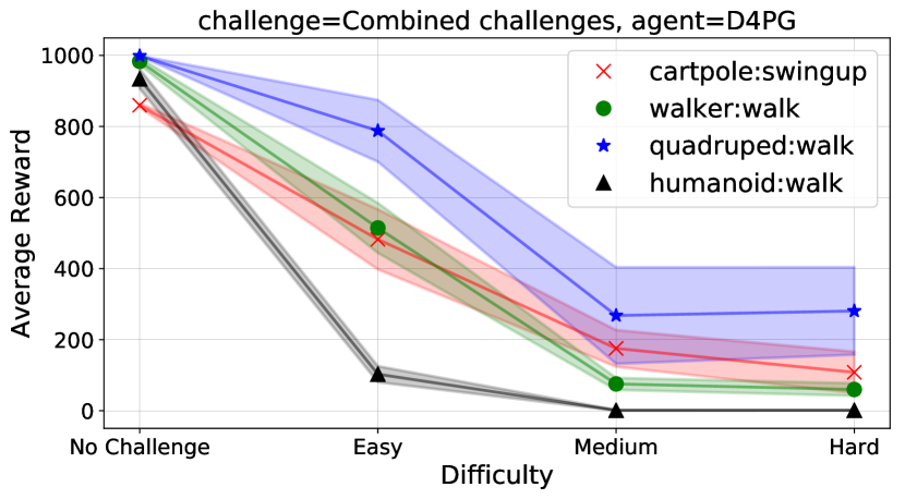
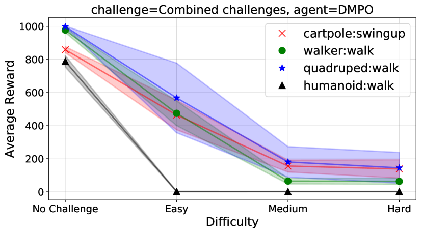
Define and baseline RWRL Combined Challenge Benchmark tasks: After careful calibration, we combine a subset of our proposed challenges into a single environment and baseline the performance of two state-of-the-art learning agents on this setup in Section 2.10. We show that state-of-the-art agents fail quickly, even for mild perturbations applied along each challenge dimension. We encourage the community to work on improving upon the combined challenges’ baseline performance. We believe that in doing so, we will take large steps towards developing agents that are implementable on real world systems.
-
•
Open-source realworldrl-suite codebase: We present the set of perturbed environments in a parametrizable suite, called realworldrl-suite which extends the DeepMind Control Suite [Tassa et al. 2018] with various perturbations representing the aforementioned challenges. The goal of the suite is to accelerate research in these areas by enabling RL practitioners and researchers to quickly, in a principled and reproducible fashion, test their learning algorithms on challenges that are encountered in many real-world systems and settings. The realworldrl-suite is available for download here: https://github.com/google-research/realworldrl_suite. A user manual, found in Appendix C, explains how to instantiate each challenge and also provides code examples for training an agent.
2 Analysis of the Real-World Challenges
In this section, for each of the challenges presented in the introduction we discuss its importance and present current research directions that attempt to tackle the challenge, providing starting points for practitioners and newcomers to the domain. We then define it more formally, and analyse its effects on state-of-the-art learning algorithms using the realworldrl-suite, to provide insights on how these challenges manifest themselves in isolation. While not all of these challenges are present together in every real system, for many systems they are all present together to some degree. For this reason, in Section 2.10 we also present a set of combined reference challenges, varying in difficulty, that emulate a complete system with all of the introduced challenges. We believe that a learner able to tackle these combined challenges would be a good candidate for many real-world systems.
Notation
Environments are formalised as Markov Decision Processes (MDPs). A MDP can be defined as a tuple , where an agent is in a state and takes an action at timestep . When in state and taking an action , an agent will arrive in a new state with probability , and receive a reward . Our environments are episodic, which is to say that they last a finite number of timesteps, . The value of , the discount factor, reflects the agent’s planning horizon. The full state of the process, , respects the Markov property: , i.e. all necessary information to predict is contained in and . In many of the environments in this paper the observed state does not include the full internal state of the MuJoCo physics simulator. It has nevertheless been shown empirically that the observed state is sufficient to control an agent, so we interchange the notion of state and observation unless otherwise specified.
Ultimately, the goal of a RL agent is to find an optimal policy which maximizes its expected return over a given MDP:
There are many ways to find this policy [Sutton and Barto 2018], and we will use two model-free methods described in the following section.
Learning algorithms:
For each challenge, we present the results of two state-of-the-art (SOTA) RL learning algorithms: Distributional Maximum a Posteriori Policy Optimization (DMPO) [Abdolmaleki et al. 2018a] and Distributed Distributional Deterministic Policy Gradient (D4PG) [Barth-Maron et al. 2018]. We chose these two algorithms for benchmarking performance as they (1) yield SOTA performance on the dm-control suite (see e.g., Hoffman et al. [2020]; Barth-Maron et al. [2018]); (2) they are both fundamentally different algorithms (DMPO is an EM-style policy iteration algorithm with a stochastic policy and D4PG is a deterministic policy gradient algorithm). Note that we also tested the original non-distributional algorithm MPO and found performance to be similar to DMPO. As such we did not include the results. It was important that our algorithms were both strong in terms of performance and diverse in terms of algorithmic implementation to show that SOTA algorithms struggle on many of the challenges that we present in the paper. We could have included more algorithms such as SAC and PPO. However, we felt that the environmental cost of running thousands of additional experiments would not justify the additional insights gained. One of our main motivations in this work is to show that SOTA algorithms do suffer from these challenges to encourage more research on these topics.
D4PG is a modified version of Deep Deterministic Policy Gradients (DDPG) [Lillicrap et al. 2015], an actor-critic algorithm where state-action values are estimated by a critic network, and the actor network is updated with gradients sampled from the critic network. D4PG makes four changes to improve the critic estimation (and thus the policy): evaluating -step rather than 1-step returns, performing a distributional critic update [Bellemare et al. 2017], using prioritized sampling of the replay buffer, and performing distributed training. These improvements give D4PG state of the art results across many DeepMind control suite [Tassa et al. 2018] tasks as well as manipulation and parkour tasks [Heess et al. 2017]. The hyperparameters for D4PG can be found in Appendix A, Table 9.
MPO [Abdolmaleki et al. 2018b] is an RL method that combines the sample efficiency of off-policy methods with the scalability and hyperparameter robustness of on-policy methods. It is an EM style method, which alternates an E-step that re-weights state-action samples with an M step that updates a deep neural network with supervised training. MPO achieves state of the art results on many continuous control tasks while using an order of magnitude fewer samples when compared with PPO [Schulman et al. 2017]. Distributional MPO (DMPO) is an extension of MPO that uses a distributional value function and achieves superior performance. The hyperparameters for DMPO can be found in Appendix A, Table 10. The hyperparameters were found by doing a grid-search on each algorithm, based on parameters used in the original papers. The algorithms achieved optimal reported performance in each case using these parameters in the ‘no challenge’ setting (i.e., when none of the challenges are present in the environment).
Each algorithm is run for K episodes on different seeds on cartpole:swingup, walker:walk, quadruped:walk and humanoid:walk tasks from the realworldrl-suite. Unless stated otherwise, the mean value reported in each graph is the mean performance of the last episodes of training with the corresponding standard deviation. All hyperparameters for all experiments can be found in Table 11. To make experiments more easily reproducible we did not use distributed training for either D4PG or DMPO. Additionally, unless otherwise noted, evaluation is performed on the same policy as used for training, to be consistent with the notion that there is no train/eval dichotomy. We refer to average reward and average return interchangeably in this paper.
2.1 Challenge 1: Learning On the Real System from Limited Samples
Motivation & Related Work
Almost all real-world systems are either slow-moving, fragile, or expensive enough to operate, that data they produce is costly and therefore learning algorithms must be as data-efficient as possible. Unlike much of the research performed in RL [Mnih et al. 2015; Espeholt et al. 2018a; Hester et al. 2018a; Tessler et al. 2016], real systems do not have separate training and evaluation environments, therefore the agent must quickly learn to act reasonably and safely. In the case where there are off-line logs of the system, these might not contain anywhere near the amount of data or data coverage that current RL algorithms expect. In addition, as all training data comes from the real system, learning agents cannot have an overly aggressive exploration policy during training, as these exploratory actions are rarely without consequence. This results in training data that is low-variance with very little of the state and action space being covered.
Learning iterations on a real system can take a long time, as slower systems’ control frequencies can range from hours in industrial settings, to multiple months in cases with infrequent user interactions such as healthcare or advertisement. Even in the case of higher-frequency control tasks, the learning algorithm needs to learn quickly from potential mistakes without having to repeat them multiple times. In addition, since there is often only one instance of the system, approaches that instantiate hundreds or thousands of environments to accelerate training through distributed training [Horgan et al. 2018; Espeholt et al. 2018b; Adamski et al. 2018] nevertheless require as much data and are rarely compatible with real systems. For all these reasons, learning on a real system requires an algorithm to be both sample-efficient and quickly performant.
There are a number of related works that deal with RL on real systems and, in particular, focus on sample efficiency. One body of work is Model Agnostic Meta-Learning (MAML) [Finn et al. 2017], which focuses on learning within a task distribution and, with few-shot learning, quickly adapting to solving a new in-distribution task that it has not seen previously. Bootstrap DQN [Osband et al. 2016] learns an ensemble of Q-networks and uses Thompson Sampling to drive exploration and improve sample efficiency. Another approach to improving sample efficiency is to use expert demonstrations to bootstrap the agent, rather than learning from scratch. This approach has been combined with DQN [Mnih et al. 2015] and demonstrated on Atari [Hester et al. 2018a], as well as combined with DDPG [Lillicrap et al. 2015] for insertion tasks on robots [Vecerík et al. 2019]. Recent Model-based deep RL approaches [Hafner et al. 2018; Chua et al. 2018; Nagabandi et al. 2019], where the algorithm plans against a learned transition model of the environment, show a lot of promise for improving sample efficiency. Haarnoja et al. [2018] introduce soft actor-critic algorithms which achieve state-of-the-art performance in terms of sample efficiency and asymptotic performance. Riedmiller et al. [2018] propose Schedule Auxiliary Control (SAC-X) that enables an agent to learn complex behaviours from scratch using multiple sparse reward signals. This leads to efficient exploration which is important for sparse reward RL. Levine and Koltun [2013] use trajectory optimization to direct policy learning and avoid poor local optima. This leads to sample efficient learning that significantly outperforms the state of the art. Yahya et al. [2017] build on this work to perform distributed learning with multiple real-world robots to achieve better sample efficiency and generalization performance on a door opening task using four robots. Another common approach is to learn ensembles of transition models and use various sampling strategies from those models to drive exploration and improve sample efficiency [Hester and Stone 2013; Chua et al. 2018; Buckman et al. 2018].
Experimental Setup & Results
To evaluate this challenge, we measure the global normalized regret with respect to the performance of the best converged policy (across algorithms). Let be the size of a sliding window across episodes where is the index of the earliest episode contained in the window. We calculate the highest average return across all algorithms using the final steps of training and denote this value . We also calculate the confidence interval for this window: . We denote as the sliding window for which more than 50% of episodes have a return higher than , and consider an agent to have converged at episode . If this condition is not satisfied during training, then , where is the total number of episodes. We can then define the global normalized regret as
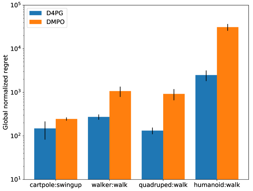
which can be read as sum of regrets for each episode , i.e., the return that would have been achieved by the best final policy minus the actual return that was achieved. The normalized regret for each of the evaluation domains is shown in Figure 1(a). The normalized regret can effectively be interpreted as the amount of actual return lost, prior to convergence, due to poor policy performance. We can observe that DMPO has higher normalized regret than D4PG on all tasks.
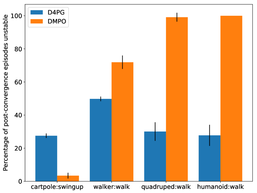
Another interesting aspect to measure upon convergence is the instability of the converged policy during training. To do so, we define the post-convergence instability, which measures the percentage of post-convergence episodes for which the return is below . This can be written as: where is an indicator function.
The average post-convergence instability for each of the domains111Note that there are no error bars for humanoid because none of the runs converge to the best performance across algorithms. is shown in Figure 1(b). As can be seen in the figure, DMPO also has higher instability than D4PG, except for cartpole:swingup.
The regret and instability metrics together can be used to summarize the sample efficiency of different algorithms. Note that they are both computed with respect to the best known performance for each task. This means that, if a new algorithm is developed that has better performance, the values of these metrics will change as a result. This is by design: when a better method comes along, it should heighten the regret of the previous ones. Note that we could have used the best possible performance for each task instead of the performance of the best known policy, but if we did that we would have run the risk that no algorithm converged to that value, making the regret potentially unbounded. We could also have normalized each algorithm by its own final performance, but that would have made it hard to compare across algorithms.
The results not only show D4PG to be generally more sample efficient, but can also be used to compare the difficulty of achieving sample efficient learning across domains. For instance, it is interesting that while D4PG takes longer to get to a policy on humanoid:walk, the policy it eventually converges to is more stable than the one for walker:walk. We hope that analysing algorithms in this way will enable a practitioner to (1) develop algorithms that are sample efficient and reduce the regret until convergence; and (2) ensure that, once converged, the algorithm is stable. These two properties are highly desirable in many industrial systems.
2.2 Challenge 2: System Delays
Motivation & Related Work
Most real systems have delays in either sensing, actuation, or reward feedback. These might occur because of low-frequency sensing and actuation, because of safety checks or other transformations performed on the selected action before it is actually implemented, or because it takes time for an action’s effect to be fully manifested.
Hester and Stone [2013] focus on controlling a robot vehicle with significant delays in the control of the braking system. They incorporate recent history into the state of the agent so that the learning algorithm can learn the delay effects itself. Mann et al. [2018] look at delays in recommender systems, where the true reward is based on the user’s interaction with the recommended item, which may take weeks to determine. They both present a factored learning approach that is able to take advantage of intermediate reward signals to improve learning in these delayed tasks. Hung et al. [2018] introduce a method to better assign rewards that arrive significantly after a causative event. They use a memory-based agent, and leverage the memory retrieval system to properly allocate credit to distant past events that are useful in predicting the value function in the current timestep. They show that this mechanism is able to solve previously unsolveable delayed reward tasks. Arjona-Medina et al. [2018] introduce the RUDDER algorithm, which uses a backwards-view of a task to generate a return-equivalent MDP where the delayed rewards are re-distributed more evenly throughout time. This return-equivalent MDP is easier to learn, is guaranteed to have the same optimal policy as the original MDP, and the approach shows improvements in Atari tasks with long delays.
Experimental Setup & Results
The realworldrl-suite implements delays in observation, action and reward with an -step buffer between the environment and the agent. An action delay is defined here as delaying the agent’s action execution for timesteps, whereas an observation/reward delay is defined as withholding an agent’s observation/reward for timesteps. We can evaluate the effects of the delay on an agent’s performance by looking at the episodic return upon convergence.
Figures 2(a) and 2(b) show the performance of D4PG and DMPO respectively under increasing levels of action, observation and reward delay. As expected, when delays increase, the performance of the algorithm decreases. Both algorithms appear to be less sensitive to reward delay compared to delays in observations or actions. This can be seen in the right-most plot of Figures 2(a) and 2(b), where the reward delay (x-axis) has to be increased to timesteps to see a significant drop in performance. The reason the agent may be more robust to reward delay is that even though the reward is delayed, it can ultimately be credited to an action that led to achieving that reward, even for relatively large delays. However, for more complicated tasks such as humanoid:walk, where action credit assignment is less obvious for large delays, performance degrades quickly. It should also be noted that the performance for observation delays is similar to that of action delays. The subtle difference between these settings is the reward that the agent receives at timestep . In the case of action delays, an agent receives the reward whereas for observation delays, the reward is .


2.3 Challenge 3: High-Dimensional Continuous State and Action Spaces
Motivation & Related Work
Many practical real-world problems have large and continuous state & action spaces. For example, consider the huge action spaces of recommender systems [Covington et al. 2016], or the number of sensors and actuators to control cooling in a data center [Evans and Gao 2016]. These large state and action spaces can present serious issues for traditional RL algorithms, (e.g., see [Dulac-Arnold et al. 2015; Tessler et al. 2019]).
There are a number of recent works focused on addressing this challenge. Dulac-Arnold et al. [2015] look at situations involving a large number of discrete actions, and present an approach based on generating a vector for a candidate action and then doing nearest neighbor search to find the closest applicable action. For systems with action cardinality that is particularly high (), it can be practical to decompose the action selection process into two steps: action candidate generation and action ranking, as detailed by Covington et al. [2016]. Zahavy et al. [2018] propose an Action Elimination Deep Q Network (AE-DQN) that uses a contextual bandit to eliminate irrelevant actions. He et al. [2015] present the Deep Reinforcement Relevance Network (DRRN) for evaluating continuous action spaces in text-based games. Tessler et al. [2019] introduce compressed sensing as an approach to reconstruct actions in text-based games with combinatorial action spaces.
| Task | Observation Dimension | Action Dimension |
|---|---|---|
| Cartpole:Swingup | 5 | 1 |
| Walker:Walk | 18 | 6 |
| Quadruped:Walk | 78 | 12 |
| Humanoid:Walk | 67 | 21 |
Experimental Setup & Results
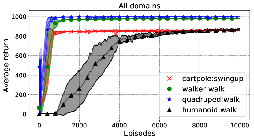
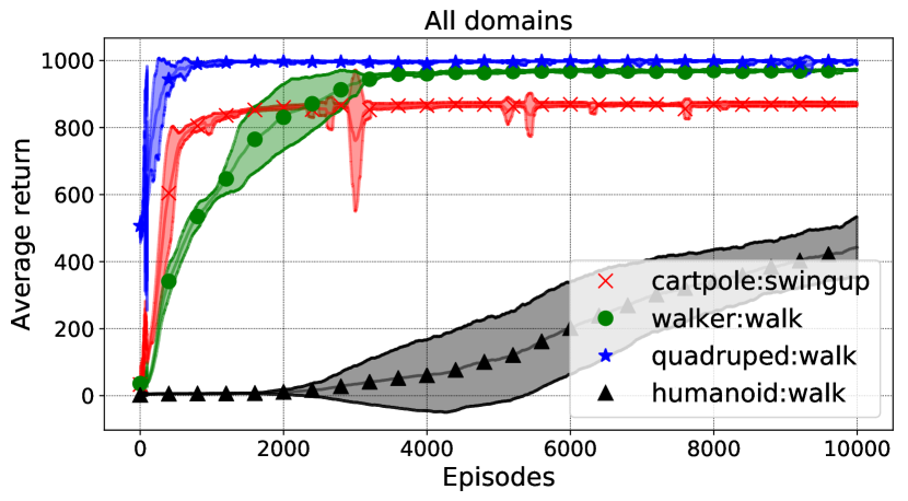
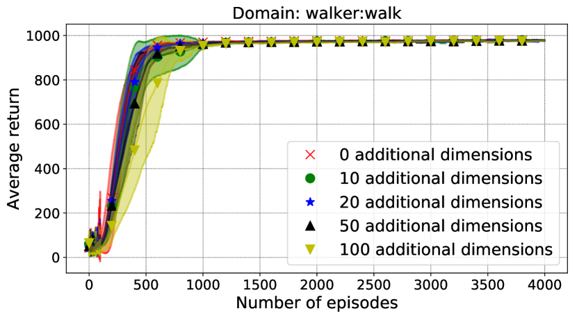
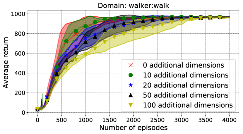
Given the continuous nature of the realworldrl-suite we chose to simulate a high-dimensional state space, although increasing the action space with dummy dimensions could be interesting for further work. For readers interested in experiments dealing with large discrete action spaces, please refer to [Dulac-Arnold et al. 2015] for various experimental setups evaluating large discrete actions spaces. For this challenge, we first compared results across all the tasks in an unperturbed manner. The state and action dimensions for each task can be found in Table 1. Both stability of the overall system and the dimensionality affect learning progress. For example, as seen in Figures 3(a) and 3(b) for D4PG and DMPO respectively, quadruped is higher dimensional than walker, yet converges faster since it is a fundamentally more stable system. On the other hand, dimensionality is also a factor as cartpole, which is significantly lower-dimensional than humanoid, converges significantly faster.
We subsequently increased the number of state dimensions of each task with dummy state variables sampled from a zero mean, unit variance normal distribution. We then compare the average return for each task as we increase the state dimensionality. Figures 4(a) and 4(b) (right) show the converged average performance of the learning algorithm on each task for D4PG and DMPO respectively. Since the added states were effectively injecting noise into the system, the algorithm learns to deal with the noise and converges to the optimal performance for the cases of cartpole:swingup, quadruped:walk and walker:walk. In some cases, e.g. Figures 5(a) and 5(b) for walker:walk, the additional dummy dimensions slightly affect convergence speed indicating that the learning algorithm learns to deal with noise efficiently, but it does slow down learning progress.


2.4 Challenge 4: Satisfying Environmental Constraints
Motivation & Related Work
Almost all physical systems can destroy or degrade themselves and the environment around them if improperly controlled. Software systems can also significantly degrade their performance or crash, as well as provide improper or incorrect interactions with users. As such, considering constraints on their operation is fundamentally necessary to controlling them. Constraints are not only important during system operation, but also during exploratory learning phases as well. Examples of physical constraints include limits on system temperatures or contact forces for safe operation, maintaining minimum battery levels, avoiding dynamic obstacles, or limiting end effector velocities. Software systems might have constraints around types of content to propose to users or system load and throughput limits to respect.
Although system designers may often wrap the learnt controller in a safety watchdog controller, the learnt controller needs to be aware of the constraints to avoid degenerate solutions which lazily rely on the watchdog. We want to emphasize that constraints can be put in place for varying reasons, ranging from monetary costs, to system up-time and longevity, to immediate physical safety of users and operators. Due to the physically grounded nature of our suite, our proposed set of constraints are physically bound and are intended to avoid self-harm, but the suite’s framework provides options for users to define any constraints they wish.
Recent work in RL safety [Dalal et al. 2018; Achiam et al. 2017; Tessler et al. 2018; Satija et al. 2020] has cast safety in the context of Constrained MDPs (CMDPs) [Altman 1999], and we will concentrate on pre-defined constraints on the environment in this context. Constrained MDPs define a constrained optimization problem and can be expressed as:
| (1) |
Here, is the cumulative reward of a policy for a given MDP, and describes the incurred cumulative cost of a certain policy relative to constraint . The CMDP framework describes multiple ways to consider cumulative cost of a policy : the total cost until task completion, the discounted cost, or the average cost. Specific constraints are defined as .
The CMDP setup allows for arbitrary constraints on state and action to be expressed. In the context of a physical system these can be as simple as box constraints on a specific state variable, or more complex such as dynamic collision-avoidance constraints. One major challenge with addressing these safety concerns in real systems is that safety violations will likely be very rare in logs of the system. In many cases, safety constraints are assumed and are not even specified by the system operator or product manager.
An extension to CMDPs is budgeted MDPs [Boutilier and Lu 2016; Carrara et al. 2018]. While for a CMDP, the constraint level is given, for budgeted MDPs, it is unknown. Instead, the policy is learned as a function of constraint level. The user can examine the trade-offs between expected return and constraint level and choose the constraint level that best works for the data. This is a good match for common real-world scenario where the constraints may not be absolute, but small violations may be allowed for a large improvement in expected returns.
Recently, there has a been a lot of work focused on the problem of safety in reinforcement learning. One focus has been the addition of a safety layer to the network [Dalal et al. 2018; Pham et al. 2017]. These approaches focus on safety during training, and have enabled an agent to learn a task with zero safety violations during training. There are other approaches [Achiam et al. 2017; Tessler et al. 2018; Bohez et al. 2019] that learn a policy that violates constraints during training but produce a trained policy that respects the safety constraints. Stooke et al. [2020] introduce the concept of lagrangian damping which leads to improved stability by performing PID control on the lagrangian parameter. Additional RL approaches include using Lyapunov functions to learn safe policies [Chow et al. 2018] and exploration strategies that predict the safety of neighboring states [Turchetta et al. 2016; Wachi et al. 2018]. Satija et al. [2020] introduce the concept of a backward value function for a more conservative optimization algorithm. A Probabilistic Goal MDP [Mankowitz et al. 2016c; Xu and Mannor 2011] is another type of objective that encourages an agent to achieve a pre-defined reward level irrespective of the time it takes to complete the task. This objective encourages risk-averse behaviour leading to safer and more robust policies. Thomas [2015] proposes a safe RL algorithm that searches for new and improved policies while ensuring that the probability of selecting bad policies is low. Calian et al. [2020] provide a meta-gradient solution to balancing the trade-off between maximizing rewards and minimizing constraint violations. This D4PG variant learns the learning rate of the lagrange multiplier in a soft-constrained optimization procedure. Thomas et al. [2017] propose a new framework for designing machine learning algorithms that simplifies the problem of specifying and regulating undesired behaviours. There have also been approaches to learn a policy that satisfies constraints in the presence of perturbations to the dynamics of an environment [Mankowitz et al. 2020].
Experimental Setup & Results
To demonstrate the complexity of system constraints, we leverage the CMDP formalism to include a series of binary safety-inspired constraints to our challenge domains. These constraints can be either considered passively, as a measure of an agent’s behavior, or they can be included in the agent’s observation so that the agent may learn to avoid them.
As an example, our cartpole environment with variables (cart position and pole angle) includes three boolean constraints:
-
1.
slider_pos, which restricts the cart’s position on the track: .
-
2.
slider_accel, which limits cart acceleration: .
-
3.
balance_velocity, a slightly more complex constraint, which limits the pole’s angular velocity when it is close to being balanced: .
The full set of available constraints across all tasks is described in Table 2. Each constraint can be tuned by modifying a parameter where is harder and is easier to satisfy.
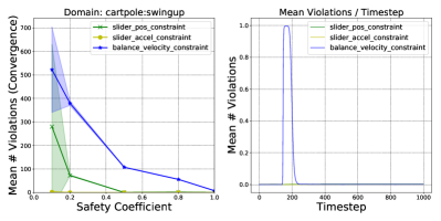
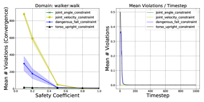
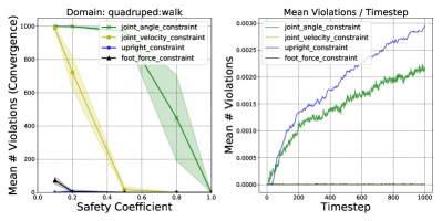
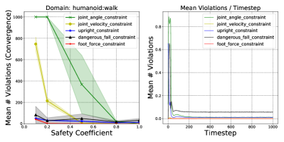
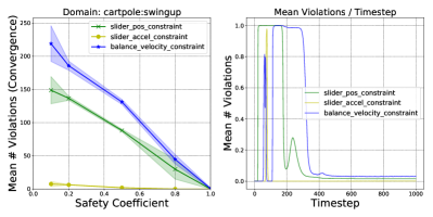
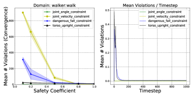
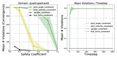
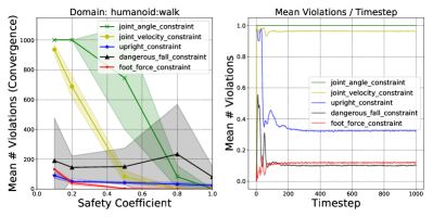
To evaluate this challenge, we track the number of constraint violations by the agent, for each constraint, throughout training. We present the effects of safety_coeff on all four environments in Figure 6. For each task, we illustrate both the effects of safety_coeff as a function of the average number of constraint violations upon convergence (left) as well as the average number of violations throughout an episode of cartpole_swingup (right). We can see that safety_coeff makes the task more difficult as it tends towards 0, and that constraint violations are non-uniform throughout time e.g. as the cart swings back and forth, the pole, position and acceleration constraints are more frequently violated.
Although the learner presented here ignores the constraints, we also include a multi-objective task which combines the task’s reward function with a constraint violation penalty in Section 2.6.
| Cart-Pole Variables: | |
|---|---|
| Type | Constraint |
| slider_pos | |
| slider_accel | |
| balance_velocity | |
| Walker Variables: | |
|---|---|
| Type | Constraint |
| joint_angle | |
| joint_velocity | |
| dangerous_fall | |
| torso_upright | |
| Quadruped Variables: | |
|---|---|
| Type | Constraint |
| joint_angle | |
| joint_velocity | |
| upright | |
| foot_force | |
| Humanoid Variables: | |
|---|---|
| Type | Constraint |
| joint_angle_constraint | |
| joint_velocity_constraint | |
| upright_constraint | |
| dangerous_fall_constraint | |
| foot_force_constraint | |
2.5 Challenge 5: Partial Observability and Non-Stationarity
Motivation & Related Work
Almost all real systems where we would want to deploy RL are partially observable. For example, on a physical system, we likely do not have observations of the wear and tear on motors or joints, or the amount of buildup in pipes or vents. We have no observations on the quality of the sensors and whether they are malfunctioning. On systems that interact with users such as recommender systems, we have no observations of the mental state of the users. Often, these partial observations appear as noise (e.g., sensor wear and tear or uncalibrated/broken sensors), non-stationarity (e.g. as a pump’s efficiency degrades) or as stochasticity (e.g. as each robot being operated behaves differently).
Partial observability.
Partially observable problems are typically formulated as a partially observable Markov Decision Process (POMDP) [Cassandra 1998]. The key difference from the MDP formulation is that the agent’s observation is now separate from the state, with an observation function giving the probability of observing given the environment state . There are a couple common approaches to handling partial observability in the literature. One is to incorporate history into the observation of the agent: DQN [Mnih et al. 2015] stacks four Atari frames together as the agent’s observation to account for partial observability. Alternatively, an approach is to use recurrent networks within the agent, enabling them to track and recover hidden state. Hausknecht and Stone [2015] apply such an approach to DQN, and show that the recurrent version can perform equally well in Atari games when only given a single frame as input. Nagabandi et al. [2018] propose an approach modeling the system as non-stationary with a time-varying reward function, and use meta-learning to find policies that will adapt to this non-stationarity. Much of the recent work on transferring learned policies from simulation to the real system also focuses on this area, as the underlying differences between the systems are not observable [Andrychowicz et al. 2018; Peng et al. 2018].
Experimental Setup & Results Many real-world sensor issues can be viewed as a partial observability challenge (unobserved properties describing the functioning of the sensor) that could be helped by recurrent models or other approaches for partial observability. A common issue we see in real-world settings is malfunctioning sensors. On any real task, we can assume that the sensors are noisy, which we reproduce by adding increasing levels of Gaussian noise to the actions and observations. Results of these perturbations can be observed in Figures 4(a) and 4(b) (left and middle figures respectively) for D4PG and DMPO. We frequently also see sensors that either get stuck at a certain value for a period of time or drop out entirely, with some default value being sent to the agent. We simulate both of these scenarios by setting both a probability of a sensor being stuck or dropped and varying the length of the malfunction being. Results for these perturbations are presented in Figures 7(a), 7(b) and Figures 8(a), 8(b) for stuck and dropped sensors. We see from the figures that both dropped and stuck sensors have a significant effect on degrading the final performance.
Non-stationarity.
Real world systems are often stochastic and noisy compared to most simulated environments. In addition, sensor and action noise as well as action delays add to the perturbations an agent may experience in the real-world setting. There are a number of RL approaches that have been utilized to ensure that an agent is robust to different subsets of these factors. We will focus on Robust MDPs, domain randomization and system identification as frameworks for reasoning about noisy, non-stationary systems.
A Robust MDP is defined by a tuple where and are as previously defined; is a set of transition matrices referred to as the uncertainty set [Iyengar 2005]. The objective that we optimize is the worst-case value function defined as:
| (2) |
At each step, nature chooses a transition function that the agent transitions with so as to minimize the long term value. The agent learns a policy that maximizes this worst case value function. Recently, a number of works have surfaced that have shown this formulation to yield robust policies that are agnostic to a range of perturbations in the environment [Tamar et al. 2014; Mankowitz et al. 2018a; Shashua and Mannor 2017; Derman et al. 2018; 2019; Mankowitz et al. 2019]. The solutions do tend to be overly conservative but some work has been done to yield less conservative, ‘soft-robust’ solutions [Derman et al. 2018].
In addition to the robust MDP formalism, the practitioner may be interested in both robustness due to domain randomization and system identification. Domain randomization [Peng et al. 2018] involves explicitly training an agent on various perturbations of the environment and averaging these learning errors together during training. System identification involves training a policy that, once on a new system, can determine the characteristics of the environment it is operating in and modify its policy accordingly [Finn et al. 2017; Nagabandi et al. 2018].
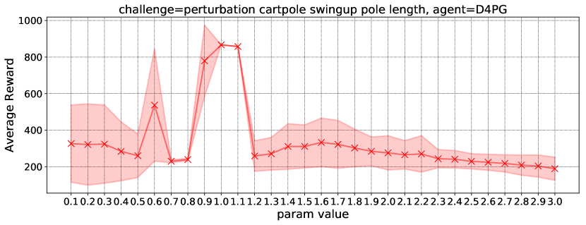
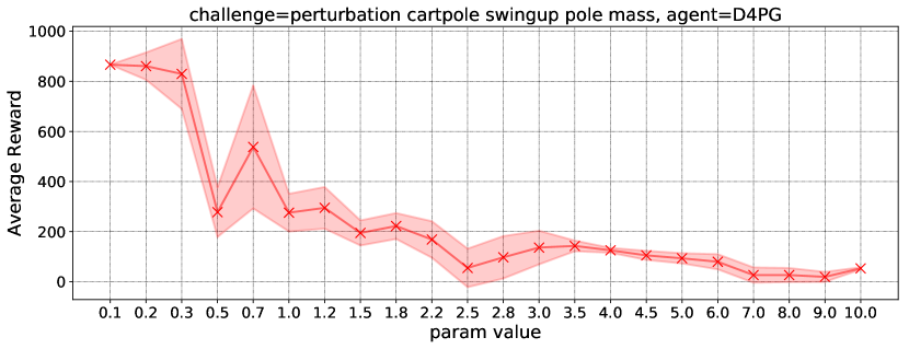
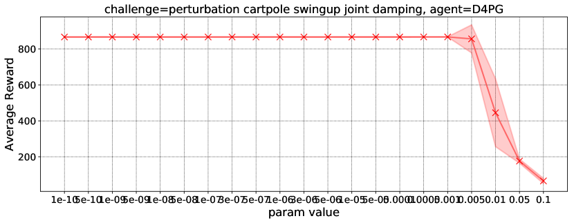
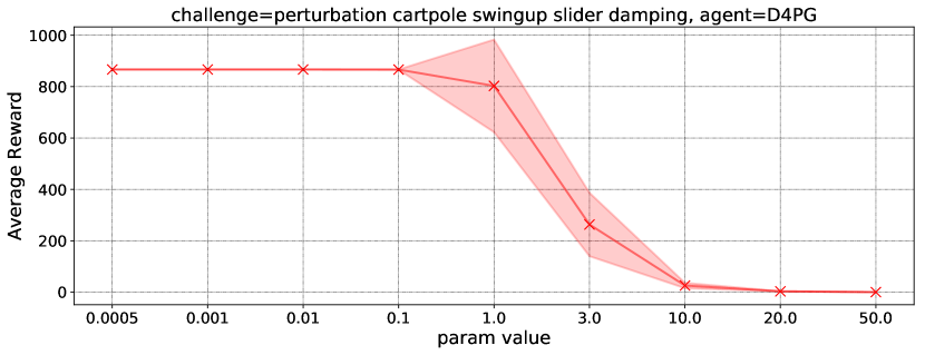
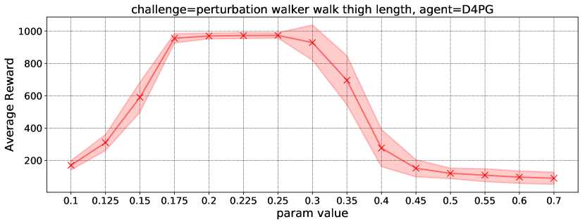
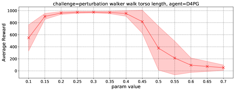
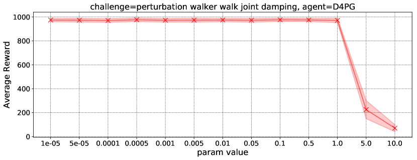
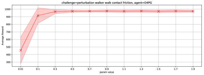
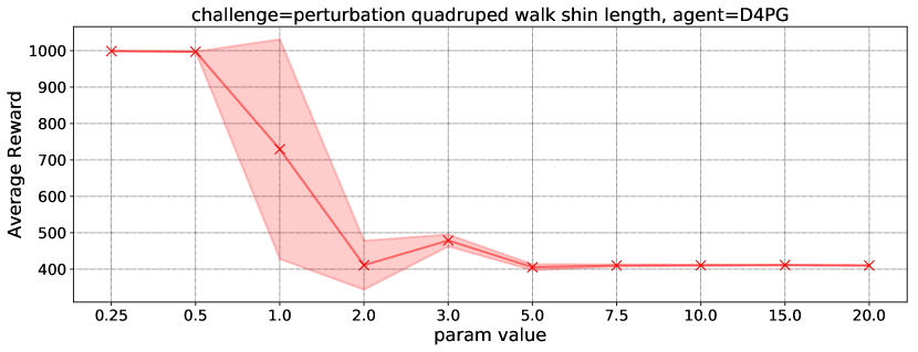
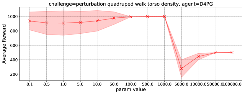
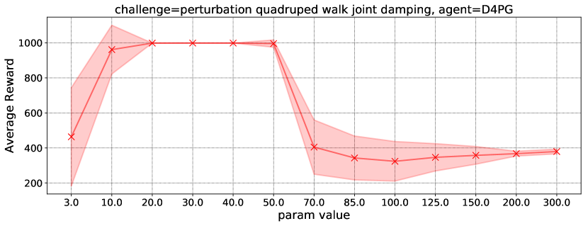
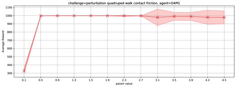
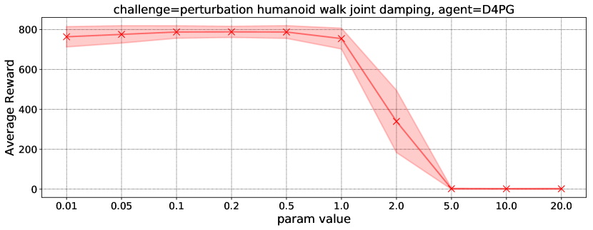
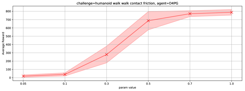
Experimental Setup & Results We perform a number of different experiments to determine the effects of non-stationarity. We first want to determine whether perturbations to the environment can have an effect on a converged policy that is trained without any challenges added to the environment. For each of the domains, we perturb each of the supported parameters shown in Table 3. The effect of the perturbations on the converged D4PG policy for each domain and supported parameter can be seen in Figure 9. It is clear that varying the perturbations does indeed have an effect on the performance of the converged policy; in many instances this causes the converged policy to completely fail. This is consistent with the results in Mankowitz et al. [2019]. This hyperparameter sweep also helps determine which parameter settings are more likely to have an effect on the learning capabilities of the agent during training.
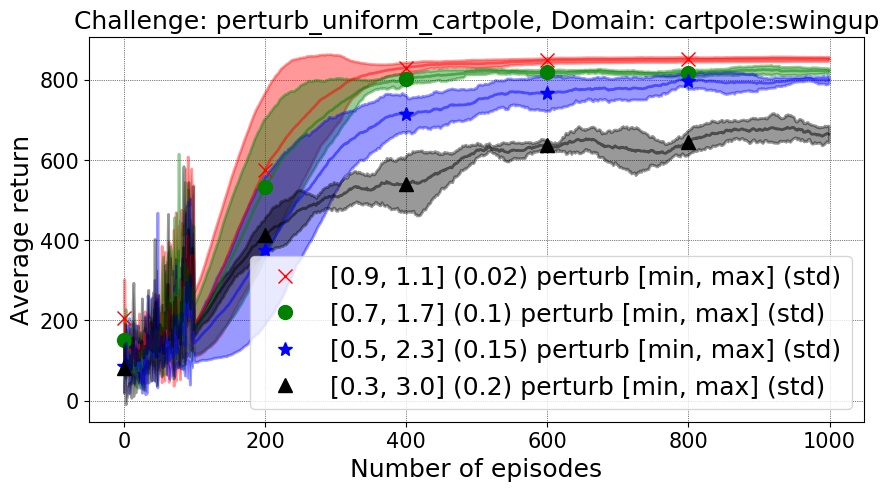
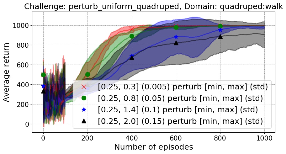
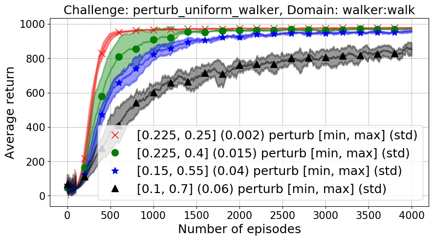
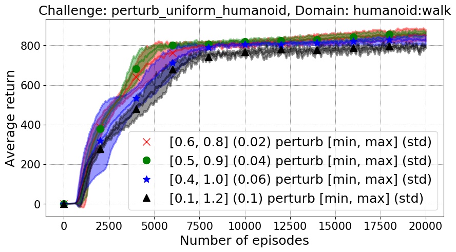
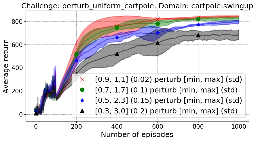
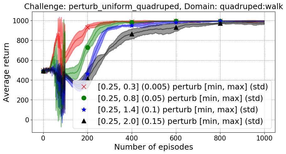
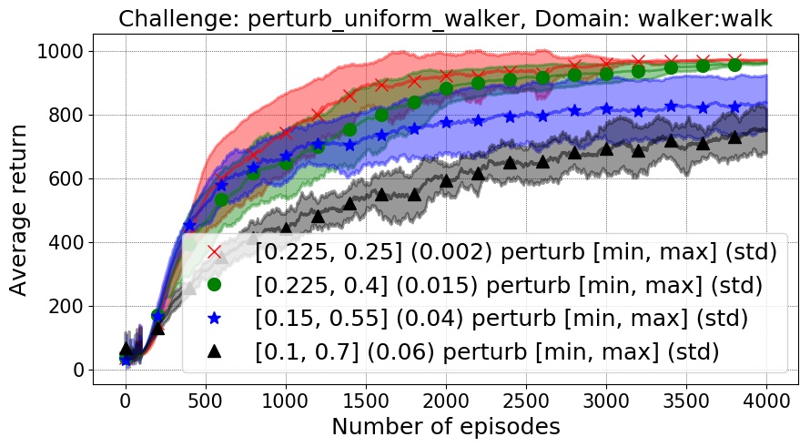
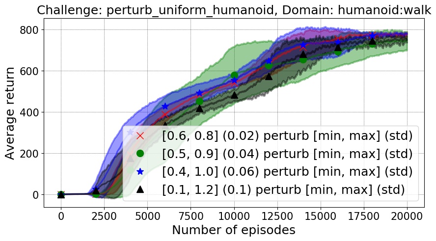
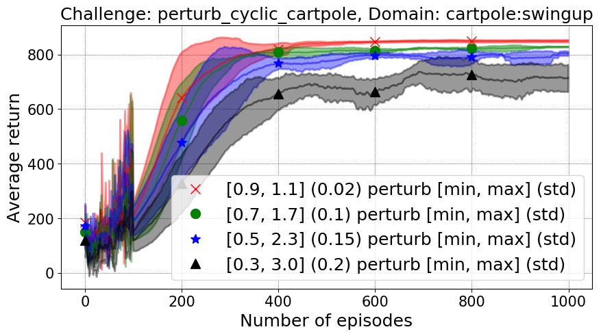
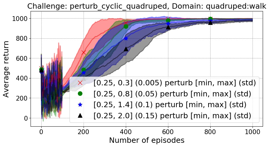
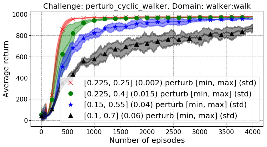
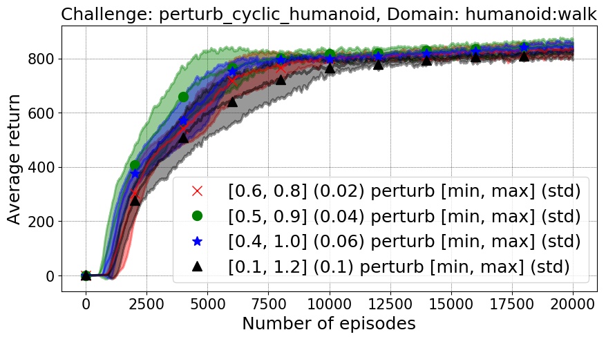
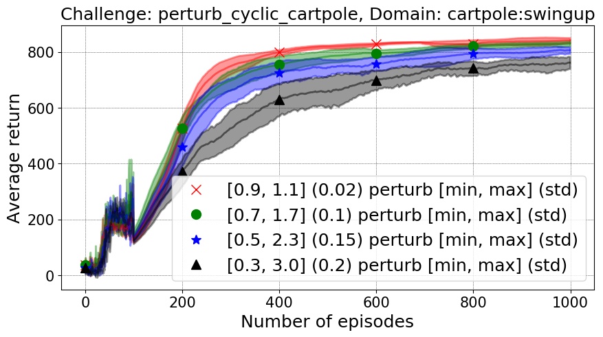
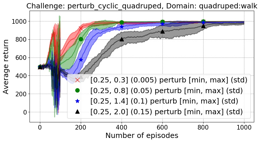
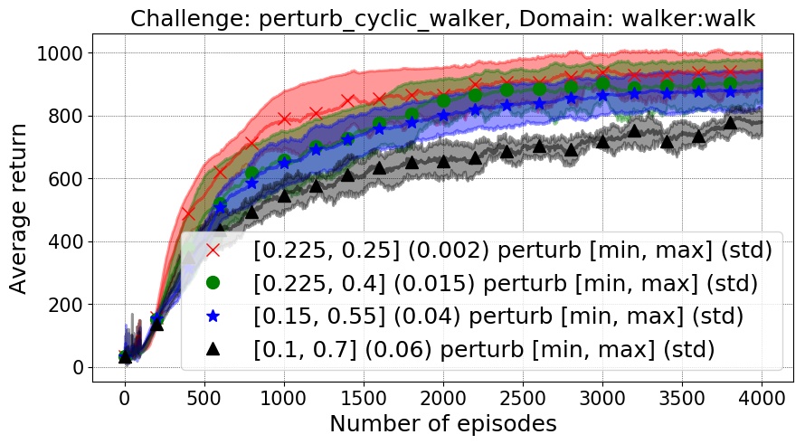
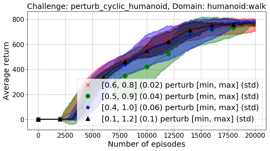
The second set of experiments therefore aim to determine the consequences of incorporating non-stationarity effects during training. Every episode, new environment parameters are sampled between a where and indicate the minimum and maximum perturbation values of a particular parameter that we vary. For example, in cartpole:swingup, the perturbation parameter is pole length and , and the variance used for sampling is .
Based on the previous set of experiments, for each task, we select domain parameters that we expect may change the optimal policy. We perform four hyperparameter training sweeps on the domain parameters for each domain & each algorithm (D4PG and DMPO). These sweeps are in increasing orders of difficulty and have thus been named , , , and are shown in Table 4. We perturb the environment in two different ways: uniform and cyclic perturbations. For uniform perturbations, we sample each episode from a uniform distribution and for the cyclic perturbations, a random positive change was sampled from a normal distribution, and the values were reset to the lower limit once the upper limit had been reached. Additional sampling methods and perturbation parameters are supported in the realworldrl-suite and can also be seen in Table 3. Cycle sampling simulates scenarios of equipment degrading over time until being replaced or fixed and returning to peak performance. The slow consistent changes over episodes also enables for the possibility of an algorithm adapting to the changes over time.
Figures 10 and 11 show the training performance for D4PG and DMPO when applying uniform and cyclic perturbations per episode respectively. As seen in the figures, increasing the range of the perturbation parameter has the effect of slowing down learning. This seems to be consistent across all of the domains we evaluated.
| Env. | Supported Parameters |
|---|---|
| Cart-Pole | Pole length |
| Pole mass | |
| Joint damping | |
| Slider damping | |
| Walker | Thigh length |
| Torso length | |
| Joint damping | |
| Contact friction | |
| Quadruped | Shin length |
| Torso density | |
| Joint damping | |
| Contact friction | |
| Humanoid | Joint Damping |
| Contact Friction | |
| Head Size |
| Env. | Default Value | |||
|---|---|---|---|---|
| Cart-Pole | ||||
| Parameter | pole_length | |||
| 0.9 | 1.1 | 0.02 | 1.0 | |
| 0.7 | 1.7 | 0.1 | 1.0 | |
| 0.5 | 2.3 | 0.15 | 1.0 | |
| 0.3 | 3.0 | 0.2 | 1.0 | |
| Walker | ||||
| Parameter | thigh_length | |||
| 0.225 | 0.25 | 0.002 | 0.225 | |
| 0.225 | 0.4 | 0.015 | 0.225 | |
| 0.15 | 0.55 | 0.04 | 0.225 | |
| 0.1 | 0.7 | 0.06 | 0.225 | |
| Quadruped | ||||
| Parameter | shin_length | |||
| 0.25 | 0.3 | 0.005 | 0.25 | |
| 0.25 | 0.8 | 0.05 | 0.25 | |
| 0.25 | 1.4 | 0.1 | 0.25 | |
| 0.25 | 2.0 | 0.15 | 0.25 | |
| Humanoid | ||||
| Parameter | join_damping | |||
| 0.6 | 0.8 | 0.02 | 0.1 | |
| 0.5 | 0.9 | 0.04 | 0.1 | |
| 0.4 | 1.0 | 0.06 | 0.1 | |
| 0.1 | 1.2 | 0.1 | 0.1 |



2.6 Challenge 6: Multi-Objective Reward Functions
Motivation & Related Work
RL frames policy learning through the lens of optimizing a global reward function, yet most systems have multi-dimensional costs to be minimized. In many cases, system or product owners do not have a clear picture of what they want to optimize. When an agent is trained to optimize one metric, other metrics are often discovered that also need to be maintained or improved. Thus, a lot of the work on deploying RL to real systems is spent figuring out how to trade off between different objectives.
There are many ways of dealing with multi-objective rewards: Roijers et al. [2013] provide an overview of various approaches. Various methods exist that deal explicitly with the multi-objective nature of the learning problems, either by predicting a value function for each objective [Van Seijen et al. 2017], or by finding a policy that optimizes each sub-problem [Li et al. 2019], or that fits each Pareto-dominating mixture of objectives [Moffaert and Nowé 2014]. Yang et al. [2019] learn a general policy that can behave optimally for any desired mixture of objectives. Multiple trivial objectives have been also used for enriching the reward signal to simply improve learning of the base task [Jaderberg et al. 2016]. Abdolmaleki et al. [2020] uses an expectation maximization approach to learn multiple Q-functions per objective.
In the specific case of dealing with balancing a task reward with negative outcomes, a possible approach is to use a Conditional Value at Risk (CVaR) objective [Tamar et al. 2015b], which looks at a given percentile of the reward distribution, rather than expected reward. Tamar et al. show that by optimizing reward percentiles, the agent is able to improve upon its worst-case performance. Distributional DQN [Dabney et al. 2018; Bellemare et al. 2017] explicitly models the distribution over returns, and it would be straight-forward to extend it to use a CVaR objective.
When rewards can’t be functionally specified, there are a number of works devoted to recovering an underlying reward function from demonstrations, such as inverse reinforcement learning [Russell 1998; Ng et al. 2000; Abbeel and Ng 2004; Ross et al. 2011]. Hadfield-Menell et al. examine how to infer the truly intended reward function from the given reward function and training MDPs, to ensure that the agent performs as intended in new scenarios.
Because the global reward function is generally a balance of multiple sub-goals (e.g., reducing both time-to-target and energy use), a proper evaluation should separate the individual components of the reward function to better understand the policy’s trade-offs. Looking at the Pareto boundaries provides some insights to the relative trade-offs between objectives, but doesn’t scale well beyond 2-3 objectives. We propose a simple multi-objective analysis of return. If we consider that the global reward function is defined as a linear combination of sub-rewards, , then we can consider the vector of per-component rewards for evaluation:
| (3) |
When dealing with multi-objective reward functions, it is important to track the different objectives individually when evaluating a policy. This allows for a more clear understanding of the different trade-offs the policy is making and choose which compromises they consider best.
To evaluate the performance of the algorithm across the full distribution of scenarios (e.g. users, tasks, robots, objects,etc.), we suggest independently analyzing the performance of the algorithm on each cohort. This is also important for ensuring fairness of an algorithm when interacting with populations of users. Another approach is to analyze the CVaR return rather than expected returns, or to directly determine whether rare catastrophic rewards are minimized [Tamar et al. 2015b; a]. Another evaluation procedure is to observe behavioural changes when an agent needs to be risk-averse or risk-seeking such as in football [Mankowitz et al. 2016c].
Experimental Setup & Results
We illustrate the multi-objective challenge by looking at the effects of a multi-objective reward function that encourages both task success and the satisfaction of safety constraints specified in Section 2.4. We use a naive mixture reward:
| (4) |
where is the task’s base reward, is the number of satisfied constraints during that timestep and is the multi-objective coefficient that balances between the objectives.
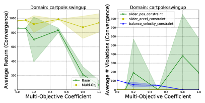
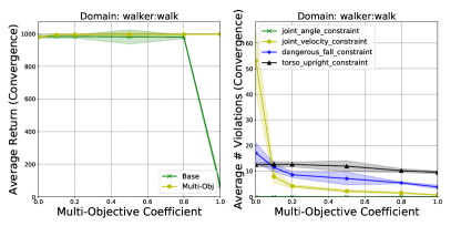
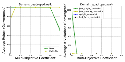
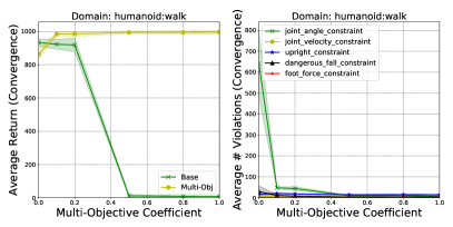
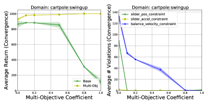
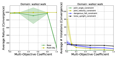
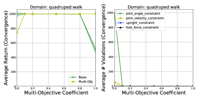
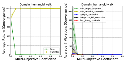
The realworldrl-suite allows multi-objective rewards to be defined, providing the multiple objectives either as observations to the agents, as modifications to the original task’s reward, or both. We use the suite to model the multi-objective problem by letting correspond to the multiobj_coeff in the realworldrl-suite, and changing the task’s reward to correspond to Equation (4). For each task, we visualize both the per-element reward, as defined in Equation (3), and the average number of each constraint’s violations upon convergence. Figure 12 shows the varying effects of this multi-objective reward on each reward component, and , as a function of multiobj_coeff, where we adjust safety_coeff to and vary multiobj_coeff. We can see the evolution in performance relative to and (left), as well as the resulting effects on constraint satisfaction (right) as multiobj_coeff is varied. As becomes more important in the global reward, constraints are quickly taken into account. However, over-emphasis on quickly degrades and therefore base task performance. Although this is a naive way to deal with safety constraints, it illustrates the often contradictory goals that a real-world task might have, and the difficulty in satisfying all of them. We also believe it provides an interesting framework to analyze how different algorithmic approaches better balance the need to satisfy constraints with the ability to maintain adequate system performance.
2.7 Challenge 7: Real-time Inference Challenge
Motivation & Related Work
To deploy RL to a production system, policy inference must be done in real-time at the control frequency of the system. This may be on the order of milliseconds for a recommender system responding to a user request [Covington et al. 2016] or the control of a physical robot, and up to the order of minutes for building control systems [Evans and Gao 2016]. This constraint both limits us from running the task faster than real-time to generate massive amounts of data quickly [Silver et al. 2016; Espeholt et al. 2018b] and limits us from running slower than real-time to perform more computationally expensive approaches (e.g. some forms of model-based planning [Doya et al. 2002; Levine et al. 2019; Schrittwieser et al. 2019]).
One approach is to take existing algorithms and validate their feasibility to run in real-time [Adam et al. 2011]. Another approach is to design algorithms with the explicit goal of running in real-time [Cai et al. 2017; Wang and Yuan 2015]. Recently Ramstedt and Pal [2019] presented a different view on real-time inference and proposed the Real-Time Markov Reward Process, in which the state evolves during an action selection. Anytime inference [Vlasselaer et al. 2015; Spirtes 2001] is a family of algorithms that can return a valid solution at any time they are being interrupted, and are expected to produce better performing solutions the longer they run. Travnik et al. [2018] propose a class of reactive SARSA RL algorithms that address the problem of asynchronous environments which occur in many real-world tasks. That is, the state is continuously changing while the agent is computing an action to take, or executing an action.
Experimental Setup & Results
The realworldrl-suite offers two ways in which one can measure the effect of real-time inference: latency and throughput. Latency corresponds to the amount of time it takes an agent to output an action based on an observation. Even if the agent is replicated over multiple machines, allowing it to handle the frequency of the observations arriving from the system, it still may have latency issues due to the time it needs in order to output an action for a single observation. To be able to see how a system will react in the face of latency, we use the action delay mechanism, where at time step the agent outputs an action based on , but the system actually responds to , where is the delay in time steps. Throughput correspond to the frequency of input observations the agent is able to process which depends on the amount of hardware or compute that is available for it as well as the complexity of the agent itself. We modeled the effects of throughput bottlenecks as action repetition: we denote the length of the action repetition by , then at time step the agent outputs an action based on the observation , however, for the next time steps (i.e., time steps ), the agent repeats the same output . These two perturbations allow us to see how agents that have latency and throughput issues will affect their environment, and additionally can show us how well an agent can learn to plan accordingly to compensate for its computational shortcomings.
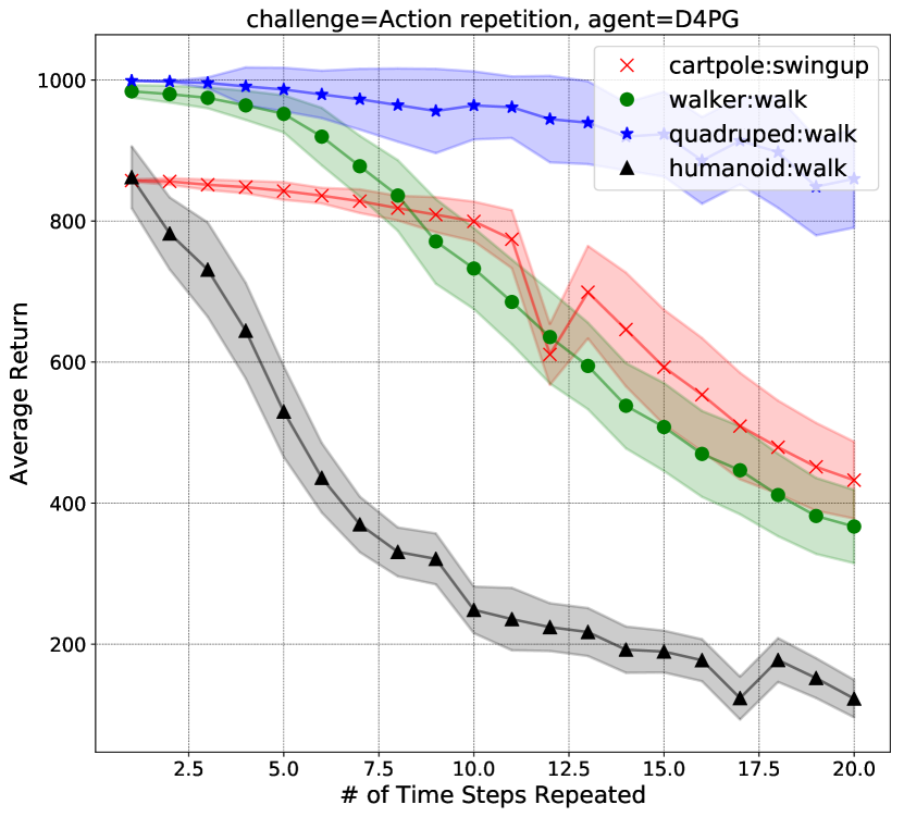
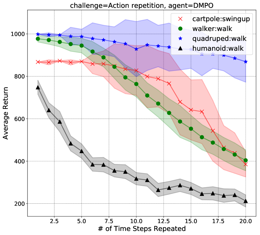
Figures 2(a) and 2(b) show the performance of D4PG and DMPO, respectively, on the action delay challenge. For discussion on these results we refer the reader to Section 2.2. Figures 13(a) and 13(b) shows the performance on the action repetition challenge for D4PG and DMPO, respectively. We note that generally, as expected, the performance of the agents deteriorates as the number of repeated actions increases. More interestingly though, we observe that albeit quadruped has larger state and action spaces than cartpole and walker, it still more robust to action repetition. We believe the reason for that lies in the inherit stability of the different tasks, where humanoid is the least stable, and quadruped is the most stable.
2.8 Challenge 8: Offline Reinforcement Learning - Training from Offline Logs
Motivation & Related Work
For many systems, learning from scratch through online interaction with the environment is too expensive or time-consuming. Therefore, it is important to design algorithms for learning good policies from offline logs of the system’s behavior. In many cases these comes from an existing rule-based, heuristic or myopic policy that we are trying to replace with an RL approach. This setting is typically referred to as Offline Reinforcement Learning 222Offline RL is also referred to as ’batch RL’ in the literature.. Offline and off-policy learning are closely related:
Off-policy learning consists of a behaviour policy that generates the data and a target policy that learns from the data generated by the behaviour policy [Sutton and Barto 2018]. The behaviour policy continuously collects data for the agent in the environment (typically a simulator). An example of this is in deep RL where data is collected using past policies up to time during training and stored in a replay buffer. This data is then used to train the policy [Levine et al. 2020]. There are numerous examples of off-policy RL such as Q-learning [Sutton and Barto 2018], Deep Q-Networks [Mnih et al. 2015] as well as actor critic variants such as IMPALA [Espeholt et al. 2018c].
Offline RL, however, does not have the luxury of a behaviour policy that continuously interacts with the environment. In this setting, a dataset of trajectories is made available to the agent from a potentially unknown behaviour policy . The dataset is collected once and is not altered during training [Levine et al. 2020].
Some of the early examples of offline RL include least squares temporal difference methods [Bradtke and Barto 1996; Lagoudakis and Parr 2003] and fitted Q iteration [Ernst et al. 2005; Riedmiller 2005]. More works such as Agarwal et al. [2019], Fujimoto et al. [2019], or Kumar et al. [2019] have shown that naively applying well-known deep RL methods such as DQN [Mnih et al. 2015] in the offline setting can lead to poor performance. This has been attributed to a combination of poor generalization outside the training data’s distribution as well as overly confident Q-function estimates when performing backups with a operator. However, distributional deep RL approaches [Dabney et al. 2018; Bellemare et al. 2017; Barth-Maron et al. 2018] have been shown to produce better performance in the offline setting in both Atari [Agarwal et al. 2019] and robot manipulation [Cabi et al. 2019]. There have also been a number of recent methods explicitly addressing the issues stemming from combining generalization outside the training data along with issues related to the operator, which come in two main flavors. The first family of approaches constrain the action choice to the support of the training data [Fujimoto et al. 2019; Kumar et al. 2019; Siegel et al. 2020; Jaques et al. 2019; Wu et al. 2019; Wang et al. 2020]. The second type of approaches start with behavior cloning [BC; Pomerleau 1989], which trains a policy using the objective of predicting the action seen in the offline logs. Works such as Wang et al. [2018], Chen et al. [2019b], or Peng et al. [2019] then use the advantage function to select the best actions in the dataset for training behavior cloning. Finally, model-based approaches also offer a solution to the offline setup, by training a model of the system dynamics offline and then exploiting it to solve the problem. Works such as MOPO [Yu et al. 2020] and MoREL [Kidambi et al. 2020] leverage the learnt model to learn a model-free policy, and approaches such as MBOP [Argenson and Dulac-Arnold 2020] leverage the model directly using an MPC-based planner.
Experimental Setup & Results
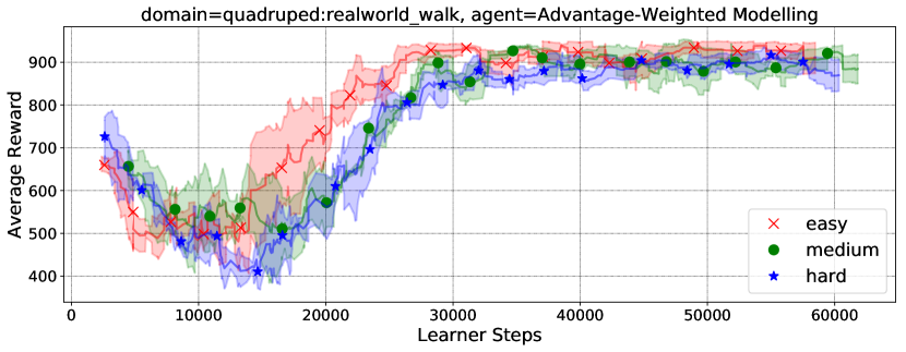
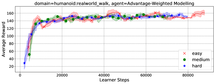
The realworldrl-suite version of the offline / batch RL challenge is to learn from data logs generated from sub-optimal policies running on the no-challenge setting, where all challenge effects are turned off, and the combined challenge setting (see Section 2.10) where data logs are generated from an environment that includes effects from combining all the challenges (except for safety and multi-objective rewards). The policies were obtained by training three DMPO agents until convergence with different random weight initializations, and then taking snapshots corresponding to roughly of the converged performance. For the no challenge setting, we generated three datasets of different sizes for each environment by combining the three snapshots, with the total dataset sizes (in numbers of episodes) provided in Table 5. Further, we repeated the procedure with the easy combination of the other challenges (see section 2.10). We chose to use the “large data” setting for the combined challenge to ensure the task is still solvable. The algorithms used for offline learning were an offline version of D4PG [Barth-Maron et al. 2018] that uses the data logs as a fixed experience replay buffer, as well as Critic Regularized Regression (CRR) Wang et al. [2020], which restricts the learned model to mimic the behavior policy when it has a positive advantage.
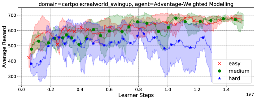
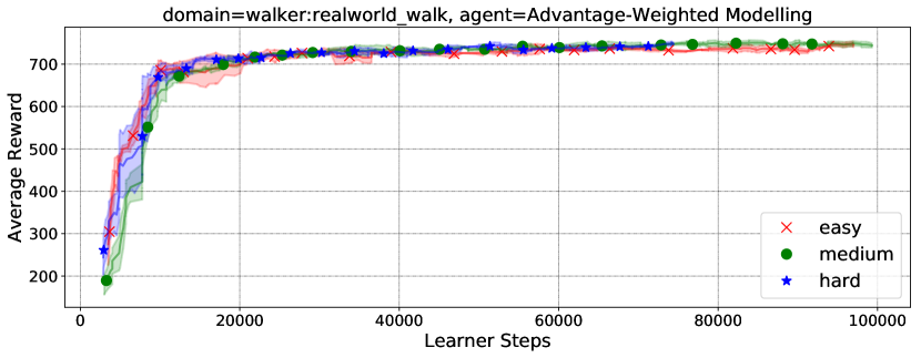
The performance of the ABM algorithm trained on the small, medium and large batch datasets can be found in Figure 14 (learning curves) for each of the domains. D4PG was also trained on each of the tasks, but failed to learn in each case and therefore the results have been omitted. As seen in the figures, the agent fails to learn properly in the humanoid:walk and cartpole:swingup domain, but manages to reach a decent level of performance in walker:walk and quadruped:walk. In addition, the size of the dataset does not seem to have a significant effect on performance. This may indicate that the dataset sizes are still too large to handicap an agent’s learning capabilities for a state-of-the-art offline RL agent, while being too difficult to solve for D4PG.
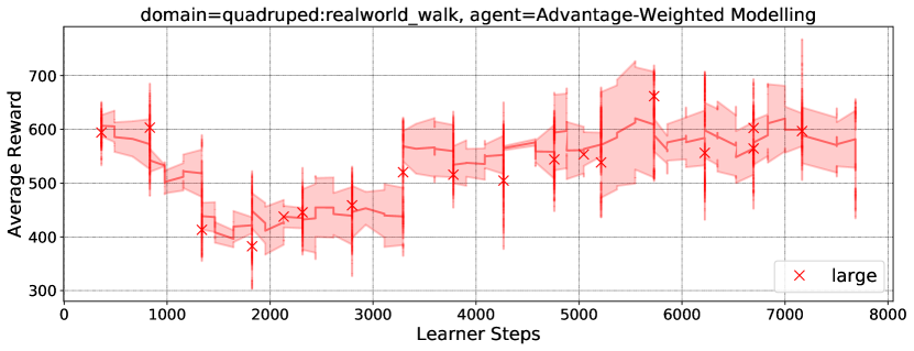
For the ‘Easy’ combined challenge offline task, we used DMPO behaviour policies trained on each task. The humanoid:walk DMPO behaviour policy was too poor to generate reasonable data (see Figure 17(b)) and we therefore focused on cartpole:swingup, walker:walk and quadruped:walk for this task. This also motivates why we need to make progress on the combined challenges online task (see Section 2.10) so that we can generate reasonable behaviour policies to generate the datasets for batch RL algorithms to train on.
We subsequently trained CRR and D4PG (offline version) on the data generated from the behaviour policies. The agents failed to achieve any reasonable level of performance on cartpole and walker, and have thus been omitted. The learning curves of CRR trained on quadruped on the combined easy challenge can be found in Figure 15. Although the performance is still sub-optimal, it is encouraging to see that the batch agents can learn something reasonable. The D4PG offline agent failed to learn in each case and the results have therefore been omitted.
| cartpole:swingup | walker:walk | quadruped:walk | humanoid:walk | |
|---|---|---|---|---|
| Small Dataset | 100 | 1000 | 100 | 4000 |
| Medium Dataset | 200 | 2000 | 200 | 8000 |
| Large Dataset | 500 | 5000 | 500 | 20000 |
2.9 Summarizing the overall performance of an agent
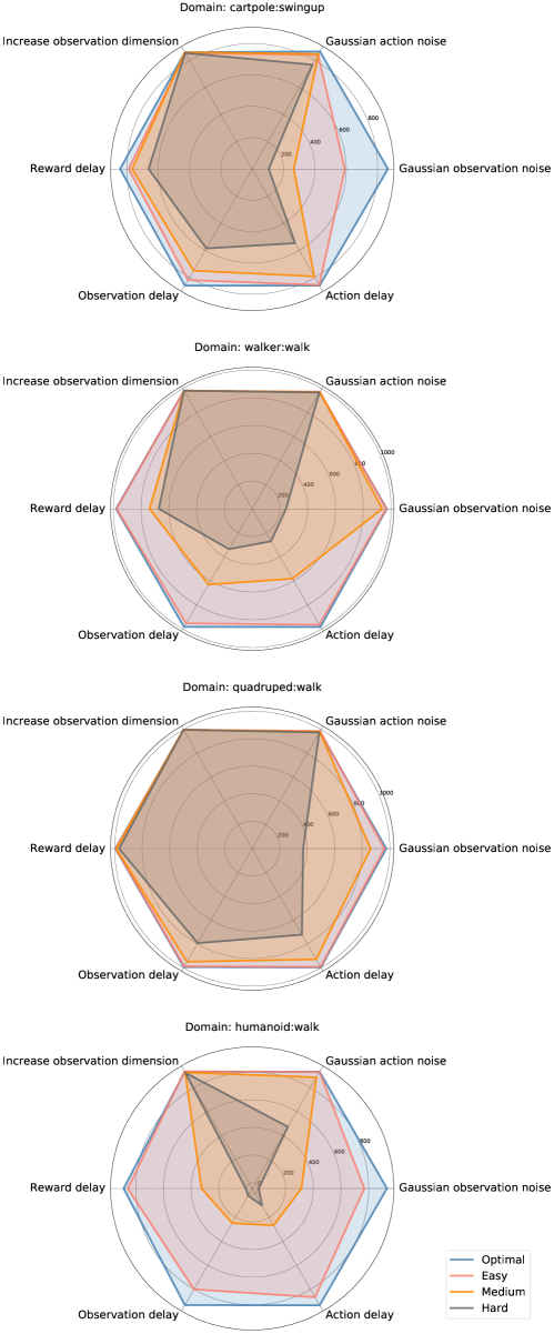
If a research or practitioner is testing out the capabilities of an agent, it would be useful to be able to summarize the performance of an agent across each challenge dimension. One such approach is to do a radar plot with respect to the various challenges. We provide an example radar plot of D4PG agent’s performance on a subset of the challenges (for visualization purposes) in Figure 16 for the domains of cartpole:swingup, walker:walk, quadruped:walk and humanoid:walk respectively. The performance is measured individually for each challenge. There are four overlapping plots on each radar plot, namely optimal performance (blue) as well as Diff1 (red), Diff2 (Orange) and Diff3 (black) which corresponds to the second, third and fourth parameters (in ascending order of difficulty) for each challenge from Table 11.
As you can see in the figure, D4PG struggles with the hard setting along each of the challenge dimensions, other than increased observation dimension. In addition it appears to be less sensitive to reward delay and adding Gaussian action noise on all domains except for humanoid. This kind of summary will immediately identify the weak points of an algorithm. We will make this plotting code available in the real-world RL suite open-source codebase.
2.10 Combining the Challenges: RWRL Benchmark
While each of these challenges present difficulties independently, many real world domains possess all of the challenges together. To demonstrate the difficulty of learning to control a system with multiple dimensions of real-world difficulty, we combine multiple challenges described above into a set of benchmark tasks to evaluate real-world learning algorithms. Our combined challenges include parameter perturbations, additional state dimensions, observation delays, action delays, reward delays, action repetition, observation & action noise, and stuck & dropped sensors. Even taking the relatively easy versions of each challenge (where the algorithm still reached close to the optimal performance individually) and combining them together creates a surprisingly difficult task. Performance on these challenges can be seen in Table 7 for D4PG and Table 8 for DMPO, and Figures 17(a) and 17(b) respectively. We can see that both learners’ performance drops drastically, even when applying the smallest perturbations of each challenge.
Due to both the application interest in these combined challenges, as well as their clear difficulty, we believe them to be good benchmark tasks for researchers looking to create RL algorithms for real-world systems. We provide the parameters for each challenge in Table 6 (taken from the individual hyperparameters sweeps, see Table 11 in the Appendix). The realworldrl-suite can load the challenges directly, making it easy to replicate these benchmark environments in any experimental setup. Although the baseline performance we provide is with a naive learner that is not designed to answer these challenges, we believe it provides a good starting point for comparison and look forward to followup work that provides more performant algorithms on these reference challenges.
| Experiment | Challenge 1 | Challenge 2 | Challenge 3 | |||
|---|---|---|---|---|---|---|
| (easy) | (Medium) | (Hard) | ||||
| System Delays | Time Steps | Time Steps | Time Steps | |||
| Action | 3 | 6 | 9 | |||
| Observation | 3 | 6 | 9 | |||
| Rewards | 10 | 20 | 40 | |||
| Action Repetition | 1 | 2 | 3 | |||
| Gaussian Noise | Std. Deviation | Std. Deviation | Std. Deviation | |||
| Action | 0.1 | 0.3 | 1.0 | |||
| Observation | 0.1 | 0.3 | 1.0 | |||
| Stuck/ | Prob. | Time | Prob. | Time | Prob. | Time |
| Dropped Noise | steps | steps | steps | |||
| Stuck Sensor | 0.01 | 1 | 0.05 | 5 | 0.1 | 10 |
| Dropped Sensor | 0.01 | 1 | 0.05 | 5 | 0.1 | 10 |
| Perturbation | [Min,Max] | Std. | [Min,Max] | Std. | [Min,Max] | Std. |
| Cartpole | ||||||
| [0.9,1.1] | 0.02 | [0.7,1.7] | 0.1 | [0.5,2.3] | 0.15 | |
| Perturbation | [Min,Max] | Std. | [Min,Max] | Std. | [Min,Max] | Std. |
| Quadruped | ||||||
| [0.25,0.3] | 0.005 | [0.25,0.8] | 0.05 | [0.25,1.4] | 0.1 | |
| Perturbation | [Min,Max] | Std. | [Min,Max] | Std. | [Min,Max] | Std. |
| Walker | ||||||
| [0.225,0.25] | 0.002 | [0.225,0.4] | 0.015 | [0.15,0.55]] | 0.04 | |
| Perturbation | [Min,Max] | Std. | [Min,Max] | Std. | [Min,Max] | Std. |
| Humanoid | ||||||
| [0.6,0.8] | 0.02 | [0.5,0.9] | 0.04 | [0.4, 1.0] | 0.06 | |
| High | State Dimension | State Dimension | State Dimension | |||
| Dimensionality | Increase | Increase | Increase | |||
| 10 | 20 | 50 | ||||
| cartpole:swingup | walker:walk | quadruped:walk | humanoid:walk | |
|---|---|---|---|---|
| 859.63 (5.68) | 983.24 (9.7) | 998.71 (0.32) | 934.0 (27.34) | |
| Easy | 482.32 (84.56) | 514.44 (70.21) | 787.73 (86.95) | 102.92 (22.47) |
| Medium | 175.47 (51.57) | 75.49 (16.94) | 268.01 (135.84) | 1.28 (0.99) |
| Hard | 108.2 (57.97) | 59.85 (17.7) | 280.75 (123.21) | 1.27 (0.79) |
| cartpole:swingup | walker:walk | quadruped:walk | humanoid:walk | |
|---|---|---|---|---|
| 859.06 (18.07) | 977.71 (14.5) | 998.35 (3.71) | 788.49 (33.88) | |
| Easy | 464.05 (89.11) | 474.44 (74.55) | 567.53 (210.54) | 1.33 (1.14) |
| Medium | 155.63 (35.81) | 64.63 (17.03) | 180.3 (92.41) | 1.27 (0.9) |
| Hard | 138.06 (55.82) | 63.05 (18.71) | 144.69 (92.85) | 1.4 (0.82) |
2.11 Future Iterations
In this paper, we have addressed 8 of the 9 challenges originally presented in [Dulac-Arnold et al. 2019]. The remaining challenge is explainability. Objectively evaluating explainability of a policy is not trivial, but we we hope this can be addressed in future iterations of this suite. We provide an overview of this challenge and possible approaches to creating explainable RL agents.
Explainability
Another essential aspect of real systems is that they are owned and operated by humans, who need to be reassured about the controllers’ intentions and require insights regarding failure cases. For this reason, policy explainability is important for real-world policies. Especially in cases where the policy might find an alternative and unexpected approach to controlling a system, understanding the longer-term intent of the policy is important for obtaining stakeholder buy-in. In the event of policy errors, being able to understand the error’s origins a posteriori is essential. Previous work that is potentially well-suited to this challenge include options [Sutton et al. 1999] that are well-defined hierarchical actions that can be composed together to solve a given task. Previous research in this area includes learning the options from scratch [Mankowitz et al. 2016a; b; Bacon et al. 2017] as well as planning, given a pre-trained set of options [Schaul et al. 2015; Mankowitz et al. 2018b]. In addition, research has been done to develop a symbolic planning language that could be useful for explainability [Konidaris et al. 2018; James et al. 2018].
2.11.1 Possible additions to the nine challenges
In addition to the nine challenges that have been defined there are a multitude of other challenges that are also up for consideration in future challenges. One such challenge is that of evolving state and action spaces. It is possible that the state space may evolve over time (e.g., adding new features to a system) as well as the action space (e.g., new capabilities are added to a robot). Instead of retraining the agent, it may be desirable to adapt the agent to the new state and action spaces.
2.11.2 Other challenges (e.g., infrastructure, societal etc)
There are also other infrastructural, societal as well as problem-dependent challenges which are not in the scope of this work. This may include code modularization; how to best allocate compute when learning under a fixed resource budget; designing simple interfaces for people with limited RL knowledge such that they can solve real-world problems; how to identify when a problem is suitable for RL. All of these challenges are also preventing RL from scaling to real-world applications at an accelerated pace. We encourage researchers and practitioners to actively think about these issues as well.
3 Additional Related Work
While we covered related work specific to each challenge in the sections above, there are a few other works that relate to ours, either through the goal of practical reinforcement learning or more generally by providing interesting benchmark suites.
In general, the fact that machine learning methods have a tendency to overfit to their evaluation environments is well-recognized. Wagstaff [2012] discusses the strong lack of real-world applications in ML conferences and the subsequent impact on research directions this can have. Henderson et al. [2018] investigate ways in which RL results can be made to be more reproducible and suggest guidelines for doing so. Their paper ends by asking the question “In what setting would [a given algorithm] be useful?”, to which we try to contribute by proposing a specific setting in which well-adapted work should hopefully stand out.
Hester and Stone [2013] similarly present a list of challenges for real world RL, but specifically for RL on robots. They present four challenges (sample efficiency, high-dimensional state and action spaces, sensor/actuator delays, and real-time inference), all of which we include in our set of challenges. They do not include our other challenges such as satisfying constraints, multi-objective, non-stationarity and partial observability (e.g., noisy/stuck sensors). Their approach is to setup a real-time architecture for model-based learning where ensembles of models are learned to improve robustness and sample efficiency. In a spirit similar to ours, the bsuite framework [Osband et al. 2019] proposes a set of challenges grounded in fundamental problems in RL such as memory, exploration, credit assignment etc. These problems are equally important and complementary to the more empirically founded challenges proposed in our suite. Recently, other teams have released real-world inspired environments, such as Safety Gym [Ray et al. 2019], which extends a planar world with location-based safety constraints. Our suite proposes a richer and more varied set of constraints, as well as an easy ability to add custom constraints, which we believe provides a more general and difficult challenge for RL algorithms.
The Horizon platform [Gauci et al. 2018] and Decision Service [Agarwal et al. 2016] provide software platforms for training, evaluation and deployment of RL agents in real-world systems. In the case of Decision Service, transition probabilities are logged to help make off-policy evaluation easier down the line, and both systems consider different approaches to off-policy evaluation. We believe well-structured frameworks such as these are crucial to productionizing RL systems. Ahn et al. [2019] propose a set of simple robot designs with corresponding simulators that have been tuned to be physically realistic, implementing safety constraints and various perturbations.
Riedmiller [2012] proposes a set of best practices for successfully solving typical real-world control tasks using RL. This is intended as a subjective report on how they tackle problems in practice.
We emphasize in this work that the goal is enable RL on real-world products and systems, which may include recommender systems, physical control systems such as autonomous driving/navigation, warehouse automation etc). There are, of course, some real-world systems that have had success using RL as the algorithmic solution - mainly in robotics. For example, Gu et al. (2017) perform off-policy training of deep Q functions to learn 3D manipulation skills as well as a door opening skill. Mahmood et al. (2018) provide benchmarks using four off-the-shelf RL algoirthms and evaluate the performance on multiple commercially available robots. Kalashnikov et al. [2018] introduce QT-Opt which is a self-supervised vision-based RL algoirthm that can learn a grasping skill that can generalize to unseen objects and handle perturbations. Levine et al. [2016] proposed an end-to-end learning algorithm that can map raw image observation’s to torques at the robot’s motors. This algorithm is able to complete a range of manipulation tasks requiring close coordination between vision and control, such as screwing a cap on a bottle.
4 Challenge Suite Overview
Our open-sourced realworldrl-suite contains:
-
•
Seven real-world challenge wrappers (mentioned above) across DeepMind Control Suite tasks [Tassa et al. 2018]:
cartpole:(swingup and balance), walker:(walk and run),
quadruped:(walk and run), humanoid:(stand and walk) -
•
The flexibility to instantiate different variants of each challenge, as well as the ability to easily combine challenges together using a simple configuration language. See Appendix C for more details.
-
•
Examples of how to run RL agents on each challenge environment.
-
•
The ability to instantiate the “Easy”, “Medium” and “Hard” combined challenges.
-
•
A Jupyter notebook enabling an agent to be run on any of the challenges in a browser, as well as accompanying functions to plot the agent’s performance.
Evaluation environments.
In this paper, we evaluate RL algorithms on a subset of four tasks from our suite, namely: cartpole:swingup, walker:walk, quadruped:walk and humanoid:walk. We chose these tasks to cover varying levels of task difficulty and dimensionality. It should be noted that MuJoCo possesses an internal dynamics state and that only preprocessed observations are available to the agent [Tassa et al. 2018]. We refer to state in this paper as in the typical MDP setting: the information available to the agent at time . Since we provide all available observations as input to the agent, we use the term observation and state interchangeably in this paper. For each challenge, we have implemented environment wrappers that instantiate the challenge. These wrappers are parameterized such that the challenge can be ramped up from having no effect to being very difficult. For example, the amount of delay added onto the actuators can be set arbitrarily, varying the difficulty from slight to impossible. By implementing the challenges in this way, we can easily adapt them to other tasks and ramp them up and down to measure their effects. Our goal with this task suite is to replicate difficulties seen in complex real systems in a more simplified setup, allowing for methodical and principled research.
5 Discussion & Conclusion
To re-iterate from the Introduction, our contributions can be structured into four parts: (1) Identifying and defining a set of challenges; (2) Designing a set of experiments and analysing their effects on common RL agents; (3) Defining and benchmarking RWRL combined challenge tasks for easy algorithmic comparisons; and (4) Open-sourcing an environmental suite, realworldrl-suite, which allows researchers and practitioners to easily replicate and extend the experiments we performed.
Identification and definition of real-world challenges
We believe that we provide a set of the most important challenges that RL algorithms need to succeed at before being ready for real-world application. In our own personal experience as well as that of our collaborators, we have been confronted ourselves numerous times with the often difficult task of applying RL to various real-world systems. This set of challenges stems from these experiences, and we are convinced that finding solutions to them will likely provide promissing algorithms that are readily useable in real-world systems. We are particularly interested in results in the off-line domain, as most large systems have a large amount of logs, but little to no tolerance for exploratory actions (datacenter cooling & robotics being good examples of this). We also believe that algorithms able to reason about environmental constraints will allow RL to move onto systems that were previously considered too fragile or expensive for learning-based approaches. Overall, we are excited about the directions that a lot of the cited research is taking and looking forward to interesting results in the near future.
Experiment design and analysis for each challenge
Additionally, the design of an experiment for each challenge demonstrates the independent effects of each challenge on an RL agent. This allowed us to show which aspects of real-world tasks present the biggest difficulties for RL agents in a precise and reproducible manner. In the case of learning on live systems from limited samples, our proposed efficiency metrics (performance regret and stability) produced interesting findings, showing DMPO to be almost an order of magnitude worse in terms of regret, but significantly more stable once converged. When dealing with system delays, we saw that observation and action delays quickly degrade algorithm performance, but reward delays seem to be globally less impactful except on the humanoid:walk task. For high-dimensional continuous state & action spaces, we see that additional observation dimensions don’t affect either DMPO or D4PG significantly, and that environments with more action dimensions are not necessarily harder to learn. When reasoning about system constraints, we argue that explicit reasoning about constraints is preferable to simply integrating them in the reward, and show that there is no natural way to express constraints in the standard MDP framework. We provide a mechanism in realworldrl-suite that can express constraints in the CMDP setting, and show that constraints can be violated in interesting ways, especially in tasks that have different regimes (e.g. cartpole:swingup’s ‘swing-up’ and ‘balance’ phases). Partial observability & non-stationarity are often present in real systems, and can present clear problems for learning algorithms. In small doses stuck sensors pose less of a problem than outright dropped signals however, even though the underlying information is the same. When it comes to non-stationary system dynamics, we can see that the effects depend greatly on the type of element that is varying. Additionally, naive policies clearly degrade more quickly in the face of unstable system dynamics. Multi-objective rewards can be difficult to optimize for when they are not well-aligned. By using safety-related constraints that weren’t always compatible with the base task, we showed how naively reasoning about this trade-off can quickly degrade system performance, yet that compromising solutions are also possible. We believe that expressing tasks beyond a single reward function is essential in tackling more complex problems and look forward to new methods able to do so. Real-time policies are essential for high-frequency control loops present in robotics or low-latency responses necessary in software systems. We showed the effects of both action and state delays on DMPO and D4PG, and showed that these approaches quickly degrade if the system’s control frequency is higher than their response time and actions decorrelate too strongly from observations. Many real-world systems are hard to train on directly, and therefore RL agents need to be able to train off-line from fixed logs. It has long been known that this is not a trivial task, as situations that aren’t represented in the data become difficult to respond to. Especially in the case of off-policy td-learning methods, the over-estimation issue quickly creates divergent value functions. We showed that simply applying D4PG to data from a logged task is not sufficient to find a functional policy, but that offline-specific learning algorithms can deal with even small amounts of data. Finally, explainable policies are often desirable (as are explainable machine learning models in general), but not easy to provide or even evaluate. We provide a couple directions of current work in this area, and hope that future work finds clearer approach to this problem.
Define and baseline RWRL Combined Challenge Benchmark tasks
By combining a well-tuned set of challenges into a single environment, we were able to generate 12 benchmark tasks (3 levels of difficulty and 4 tasks) which can serve as reference tasks for further research in real-world RL. The choice of challenge parameterizations for each level of difficulty was performed after careful analysis of the combined effects on the learning algorithms we experimented with. We also provided a first round of baselines on our benchmark tasks by running D4PG and DMPO on them: we find that D4PG seems to be slightly more robust for easy perturbations but, aside from the quadruped:walk task, quickly matches DMPO in poor performance. By providing these baseline performance numbers for D4PG and DPMO on these task, we hope that followup work will have a good starting point to understand the quality of their proposed solutions. We encourage the research community to better our current set of RWRL combined challenge baseline results.
Open-source the realworldrl-suite codebase
Finally, by implementing all our challenges in the open-sourced realworldrl-suite, we provide a reference implementation for each challenge that allows easy performance comparisons between algorithms hoping to respond to these challenges. By leveraging both the realworldrl-suite and the performance baselines for each challenge presented in this paper, future researchers developing real-world RL algorithms can easily compare their approach against common baselines to provide clear and objective evaluation.
We hope this body of works provides both encouragement to the reinforcement learning community to take up these challenges that are important holdups to bringing RL into real systems, as well as intuition to practitioners who have confronted themselves with attempting to apply RL methods on practical tasks. We strongly believe that robust, dependable, safe, efficient, scalable RL algorithms are possible, and look forward to seeing the coming years of research in this area.
References
- Abbeel and Ng [2004] P. Abbeel and A. Y. Ng. Apprenticeship learning via inverse reinforcement learning. In Proceedings of the twenty-first international conference on Machine learning, page 1. ACM, 2004.
- Abbeel et al. [2010] P. Abbeel, A. Coates, and A. Y. Ng. Autonomous helicopter aerobatics through apprenticeship learning. The International Journal of Robotics Research, 29(13):1608–1639, 2010.
- Abdolmaleki et al. [2018a] A. Abdolmaleki, J. T. Springenberg, Y. Tassa, R. Munos, N. Heess, and M. A. Riedmiller. Maximum a posteriori policy optimisation. CoRR, abs/1806.06920, 2018a.
- Abdolmaleki et al. [2018b] A. Abdolmaleki, J. T. Springenberg, Y. Tassa, R. Munos, N. Heess, and M. A. Riedmiller. Maximum a posteriori policy optimisation. In International Conference on Learning Representations (ICLR), 2018b.
- Abdolmaleki et al. [2020] A. Abdolmaleki, S. H. Huang, L. Hasenclever, M. Neunert, H. F. Song, M. Zambelli, M. F. Martins, N. Heess, R. Hadsell, and M. Riedmiller. A distributional view on multi-objective policy optimization. arXiv preprint arXiv:2005.07513, 2020.
- Achiam et al. [2017] J. Achiam, D. Held, A. Tamar, and P. Abbeel. Constrained policy optimization. CoRR, abs/1705.10528, 2017.
- Adam et al. [2011] S. Adam, L. Busoniu, and R. Babuska. Experience replay for real-time reinforcement learning control. IEEE Transactions on Systems, Man, and Cybernetics, Part C (Applications and Reviews), 42(2):201–212, 2011.
- Adamski et al. [2018] I. Adamski, R. Adamski, T. Grel, A. Jedrych, K. Kaczmarek, and H. Michalewski. Distributed deep reinforcement learning: Learn how to play atari games in 21 minutes. In International Conference on High Performance Computing, pages 370–388. Springer, 2018.
- Agarwal et al. [2016] A. Agarwal, S. Bird, M. Cozowicz, L. Hoang, J. Langford, S. Lee, J. Li, D. Melamed, G. Oshri, O. Ribas, et al. Making contextual decisions with low technical debt. arXiv preprint arXiv:1606.03966, 2016.
- Agarwal et al. [2019] R. Agarwal, D. Schuurmans, and M. Norouzi. Striving for simplicity in off-policy deep reinforcement learning. Preprint arXiv:1907.04543, 2019.
- Ahn et al. [2019] M. Ahn, H. Zhu, K. Hartikainen, H. Ponte, A. Gupta, S. Levine, and V. Kumar. ROBEL: RObotics BEnchmarks for Learning with low-cost robots. In Conference on Robot Learning (CoRL), 2019.
- Altman [1999] E. Altman. Constrained Markov decision processes, volume 7. CRC Press, 1999.
- Andrychowicz et al. [2018] M. Andrychowicz, B. Baker, M. Chociej, R. Jozefowicz, B. McGrew, J. Pachocki, A. Petron, M. Plappert, G. Powell, A. Ray, et al. Learning dexterous in-hand manipulation. arXiv preprint arXiv:1808.00177, 2018.
- Argenson and Dulac-Arnold [2020] A. Argenson and G. Dulac-Arnold. Model-based offline planning. arXiv preprint arXiv:2008.05556, 2020.
- Arjona-Medina et al. [2018] J. A. Arjona-Medina, M. Gillhofer, M. Widrich, T. Unterthiner, and S. Hochreiter. Rudder: Return decomposition for delayed rewards. arXiv preprint arXiv:1806.07857, 2018.
- Bacon et al. [2017] P.-L. Bacon, J. Harb, and D. Precup. The option-critic architecture. In Thirty-First AAAI Conference on Artificial Intelligence, 2017.
- Barth-Maron et al. [2018] G. Barth-Maron, M. W. Hoffman, D. Budden, W. Dabney, D. Horgan, D. TB, A. Muldal, N. Heess, and T. P. Lillicrap. Distributed distributional deterministic policy gradients. In International Conference on Learning Representations (ICLR), 2018.
- Bellemare et al. [2017] M. G. Bellemare, W. Dabney, and R. Munos. A distributional perspective on reinforcement learning. CoRR, abs/1707.06887, 2017.
- Bohez et al. [2019] S. Bohez, A. Abdolmaleki, M. Neunert, J. Buchli, N. Heess, and R. Hadsell. Value constrained model-free continuous control. arXiv preprint arXiv:1902.04623, 2019.
- Boutilier and Lu [2016] C. Boutilier and T. Lu. Budget allocation using weakly coupled, constrained markov decision processes. In Proceedings of the 32nd Conference on Uncertainty in Artificial Intelligence (UAI-16), pages 52–61, New York, NY, 2016.
- Bradtke and Barto [1996] S. Bradtke and A. Barto. Linear least-squares algorithms for temporal difference learning. Machine Learning, 22:33–57, 03 1996.
- Buckman et al. [2018] J. Buckman, D. Hafner, G. Tucker, E. Brevdo, and H. Lee. Sample-efficient reinforcement learning with stochastic ensemble value expansion. CoRR, abs/1807.01675, 2018.
- Cabi et al. [2019] S. Cabi, S. G. Colmenarejo, A. Novikov, K. Konyushkova, S. Reed, R. Jeong, K. Zolna, Y. Aytar, D. Budden, M. Vecerik, O. Sushkov, D. Barker, J. Scholz, M. Denil, N. de Freitas, and Z. Wang. Scaling data-driven robotics with reward sketching and batch reinforcement learning. Preprint arXiv:1909.12200, 2019.
- Cai et al. [2017] H. Cai, K. Ren, W. Zhang, K. Malialis, J. Wang, Y. Yu, and D. Guo. Real-time bidding by reinforcement learning in display advertising. In Proceedings of the Tenth ACM International Conference on Web Search and Data Mining, pages 661–670, 2017.
- Calian et al. [2020] D. A. Calian, D. J. Mankowitz, T. Zahavy, Z. Xu, J. Oh, N. Levine, and T. Mann. Balancing constraints and rewards with meta-gradient d4pg, 2020.
- Carrara et al. [2018] N. Carrara, R. Laroche, J. Bouraoui, T. Urvoy, T. D. S. Olivier, and O. Pietquin. A fitted-q algorithm for budgeted mdps. In EWRL 2018, 2018.
- Cassandra [1998] A. R. Cassandra. A survey of pomdp applications. In Working notes of AAAI 1998 fall symposium on planning with partially observable Markov decision processes, volume 1724, 1998.
- Chen et al. [2019a] M. Chen, A. Beutel, P. Covington, S. Jain, F. Belletti, and E. H. Chi. Top-k off-policy correction for a reinforce recommender system. In Proceedings of the Twelfth ACM International Conference on Web Search and Data Mining, pages 456–464, 2019a.
- Chen et al. [2019b] X. Chen, Z. Zhou, Z. Wang, C. Wang, Y. Wu, Q. Deng, and K. Ross. BAIL: Best-action imitation learning for batch deep reinforcement learning. Preprint arXiv:1910.12179, 2019b.
- Chow et al. [2018] Y. Chow, O. Nachum, E. Duenez-Guzman, and M. Ghavamzadeh. A lyapunov-based approach to safe reinforcement learning. In S. Bengio, H. Wallach, H. Larochelle, K. Grauman, N. Cesa-Bianchi, and R. Garnett, editors, Advances in Neural Information Processing Systems 31, pages 8092–8101. 2018.
- Chua et al. [2018] K. Chua, R. Calandra, R. McAllister, and S. Levine. Deep reinforcement learning in a handful of trials using probabilistic dynamics models. In Advances in Neural Information Processing Systems, pages 4754–4765, 2018.
- Covington et al. [2016] P. Covington, J. Adams, and E. Sargin. Deep neural networks for youtube recommendations. In Proceedings of the 10th ACM conference on recommender systems, pages 191–198. ACM, 2016.
- Dabney et al. [2018] W. Dabney, G. Ostrovski, D. Silver, and R. Munos. Implicit quantile networks for distributional reinforcement learning. In J. Dy and A. Krause, editors, Proceedings of the 35th International Conference on Machine Learning, volume 80 of Proceedings of Machine Learning Research, pages 1096–1105, Stockholmsmässan, Stockholm Sweden, 10–15 Jul 2018. PMLR.
- Dalal et al. [2018] G. Dalal, K. Dvijotham, M. Vecerik, T. Hester, C. Paduraru, and Y. Tassa. Safe exploration in continuous action spaces. CoRR, abs/1801.08757, 2018.
- Derman et al. [2018] E. Derman, D. J. Mankowitz, T. A. Mann, and S. Mannor. Soft-robust actor-critic policy-gradient. arXiv preprint arXiv:1803.04848, 2018.
- Derman et al. [2019] E. Derman, D. J. Mankowitz, T. A. Mann, and S. Mannor. A bayesian approach to robust reinforcement learning. CoRR, abs/1905.08188, 2019. URL http://arxiv.org/abs/1905.08188.
- Doya et al. [2002] K. Doya, K. Samejima, K.-i. Katagiri, and M. Kawato. Multiple model-based reinforcement learning. Neural computation, 14(6):1347–1369, 2002.
- Dulac-Arnold et al. [2015] G. Dulac-Arnold, R. Evans, H. van Hasselt, P. Sunehag, T. Lillicrap, J. Hunt, T. Mann, T. Weber, T. Degris, and B. Coppin. Deep reinforcement learning in large discrete action spaces. arXiv preprint arXiv:1512.07679, 2015.
- Dulac-Arnold et al. [2019] G. Dulac-Arnold, D. J. Mankowitz, and T. Hester. Challenges of real-world reinforcement learning. ICML Workshop on Reinforcement Learning for Real Life, abs/1904.12901, 2019.
- Ernst et al. [2005] D. Ernst, P. Geurts, and L. Wehenkel. Tree-based batch mode reinforcement learning. Journal of Machine Learning Research, 6:503–556, 2005.
- Espeholt et al. [2018a] L. Espeholt, H. Soyer, R. Munos, K. Simonyan, V. Mnih, T. Ward, Y. Doron, V. Firoiu, T. Harley, I. Dunning, S. Legg, and K. Kavukcuoglu. IMPALA: scalable distributed deep-rl with importance weighted actor-learner architectures. CoRR, abs/1802.01561, 2018a.
- Espeholt et al. [2018b] L. Espeholt, H. Soyer, R. Munos, K. Simonyan, V. Mnih, T. Ward, Y. Doron, V. Firoiu, T. Harley, I. Dunning, S. Legg, and K. Kavukcuoglu. IMPALA: Scalable distributed deep-RL with importance weighted actor-learner architectures. In J. Dy and A. Krause, editors, Proceedings of the 35th International Conference on Machine Learning, volume 80 of Proceedings of Machine Learning Research, pages 1407–1416, Stockholmsmässan, Stockholm Sweden, 10–15 Jul 2018b. PMLR.
- Espeholt et al. [2018c] L. Espeholt, H. Soyer, R. Munos, K. Simonyan, V. Mnih, T. Ward, Y. Doron, V. Firoiu, T. Harley, I. Dunning, et al. Impala: Scalable distributed deep-rl with importance weighted actor-learner architectures. arXiv preprint arXiv:1802.01561, 2018c.
- Evans and Gao [2016] R. Evans and J. Gao. Deepmind ai reduces google data centre cooling bill by 40%, 2016. URL https://deepmind.com/blog/deepmind-ai-reduces-google-data-centre-cooling-bill-40/.
- Finn et al. [2017] C. Finn, P. Abbeel, and S. Levine. Model-agnostic meta-learning for fast adaptation of deep networks. In Proceedings of the 34th International Conference on Machine Learning-Volume 70, pages 1126–1135. JMLR. org, 2017.
- Fujimoto et al. [2019] S. Fujimoto, D. Meger, and D. Precup. Off-policy deep reinforcement learning without exploration. In International Conference on Machine Learning, pages 2052–2062, 2019.
- Gauci et al. [2018] J. Gauci, E. Conti, Y. Liang, K. Virochsiri, Y. He, Z. Kaden, V. Narayanan, and X. Ye. Horizon: Facebook’s open source applied reinforcement learning platform. arXiv preprint arXiv:1811.00260, 2018.
- Gu et al. [2017] S. Gu, E. Holly, T. Lillicrap, and S. Levine. Deep reinforcement learning for robotic manipulation with asynchronous off-policy updates. In 2017 IEEE international conference on robotics and automation (ICRA), pages 3389–3396. IEEE, 2017.
- Haarnoja et al. [2018] T. Haarnoja, A. Zhou, K. Hartikainen, G. Tucker, S. Ha, J. Tan, V. Kumar, H. Zhu, A. Gupta, P. Abbeel, et al. Soft actor-critic algorithms and applications. arXiv preprint arXiv:1812.05905, 2018.
- Hadfield-Menell et al. [2017] D. Hadfield-Menell, S. Milli, P. Abbeel, S. J. Russell, and A. D. Dragan. Inverse reward design. CoRR, abs/1711.02827, 2017.
- Hafner et al. [2018] D. Hafner, T. Lillicrap, I. Fischer, R. Villegas, D. Ha, H. Lee, and J. Davidson. Learning latent dynamics for planning from pixels. arXiv preprint arXiv:1811.04551, 2018.
- Hausknecht and Stone [2015] M. J. Hausknecht and P. Stone. Deep recurrent q-learning for partially observable mdps. CoRR, abs/1507.06527, 2015.
- He et al. [2015] J. He, J. Chen, X. He, J. Gao, L. Li, L. Deng, and M. Ostendorf. Deep reinforcement learning with a natural language action space. arXiv preprint arXiv:1511.04636, 2015.
- Heess et al. [2017] N. Heess, D. TB, S. Sriram, J. Lemmon, J. Merel, G. Wayne, Y. Tassa, T. Erez, Z. Wang, S. Eslami, et al. Emergence of locomotion behaviours in rich environments. arXiv preprint arXiv:1707.02286, 2017.
- Henderson et al. [2018] P. Henderson, R. Islam, P. Bachman, J. Pineau, D. Precup, and D. Meger. Deep reinforcement learning that matters. In Thirty-Second AAAI Conference on Artificial Intelligence, 2018.
- Hester and Stone [2013] T. Hester and P. Stone. TEXPLORE: Real-time sample-efficient reinforcement learning for robots. Machine Learning, 90(3), 2013. doi: 10.1007/s10994-012-5322-7.
- Hester et al. [2018a] T. Hester, M. Vecerik, O. Pietquin, M. Lanctot, T. Schaul, B. Piot, D. Horgan, J. Quan, A. Sendonaris, I. Osband, G. Dulac-Arnold, J. Agapiou, J. Z. Leibo, and A. Gruslys. Deep q-learning from demonstrations. In Proceedings of the Thirty-Second AAAI Conference on Artificial Intelligence, (AAAI-18), pages 3223–3230, 2018a.
- Hester et al. [2018b] T. A. Hester, E. J. Fisher, and P. Khandelwal. Predictively controlling an environmental control system, Jan. 16 2018b. US Patent 9,869,484.
- Hoffman et al. [2020] M. Hoffman, B. Shahriari, J. Aslanides, G. Barth-Maron, F. Behbahani, T. Norman, A. Abdolmaleki, A. Cassirer, F. Yang, K. Baumli, et al. Acme: A research framework for distributed reinforcement learning. arXiv preprint arXiv:2006.00979, 2020.
- Horgan et al. [2018] D. Horgan, J. Quan, D. Budden, G. Barth-Maron, M. Hessel, H. van Hasselt, and D. Silver. Distributed prioritized experience replay. CoRR, abs/1803.00933, 2018.
- Hung et al. [2018] C.-C. Hung, T. Lillicrap, J. Abramson, Y. Wu, M. Mirza, F. Carnevale, A. Ahuja, and G. Wayne. Optimizing agent behavior over long time scales by transporting value. arXiv preprint arXiv:1810.06721, 2018.
- Ie et al. [2019] E. Ie, C.-w. Hsu, M. Mladenov, V. Jain, S. Narvekar, J. Wang, R. Wu, and C. Boutilier. Recsim: A configurable simulation platform for recommender systems. arXiv preprint arXiv:1909.04847, 2019.
- Iyengar [2005] G. N. Iyengar. Robust dynamic programming. Mathematics of Operations Research, 30(2):257–280, 2005.
- Jaderberg et al. [2016] M. Jaderberg, V. Mnih, W. Czarnecki, T. Schaul, J. Z. L. Leibo, D. Silver, and K. Kavukcuoglu. Reinforcement Learning with Unsupervised Auxiliary Tasks. arXiv, pages 1–11, 2016. ISSN 0004-6361. doi: 10.1051/0004-6361/201527329.
- James et al. [2018] S. James, B. Rosman, and G. Konidaris. Learning to plan with portable symbols. In Workshop on Planning and Learning (PAL@ ICML/IJCAI/AAMAS), 2018.
- Jaques et al. [2019] N. Jaques, A. Ghandeharioun, J. H. Shen, C. Ferguson, À. Lapedriza, N. Jones, S. Gu, and R. W. Picard. Way off-policy batch deep reinforcement learning of implicit human preferences in dialog. Preprint arXiv:1907.00456, 2019.
- Kalashnikov et al. [2018] D. Kalashnikov, A. Irpan, P. Pastor, J. Ibarz, A. Herzog, E. Jang, D. Quillen, E. Holly, M. Kalakrishnan, V. Vanhoucke, et al. Qt-opt: Scalable deep reinforcement learning for vision-based robotic manipulation. arXiv preprint arXiv:1806.10293, 2018.
- Kidambi et al. [2020] R. Kidambi, A. Rajeswaran, P. Netrapalli, and T. Joachims. Morel: Model-based offline reinforcement learning. arXiv preprint arXiv:2005.05951, 2020.
- Konidaris et al. [2018] G. Konidaris, L. P. Kaelbling, and T. Lozano-Perez. From skills to symbols: Learning symbolic representations for abstract high-level planning. Journal of Artificial Intelligence Research, 61:215–289, 2018.
- Kumar et al. [2019] A. Kumar, J. Fu, M. Soh, G. Tucker, and S. Levine. Stabilizing off-policy Q-learning via bootstrapping error reduction. In Conference on Neural Information Processing Systems, pages 11761–11771, 2019.
- Lagoudakis and Parr [2003] M. G. Lagoudakis and R. Parr. Least-squares policy iteration. Journal of Machine Learning Research, 4:1107–1149, 2003.
- Levine et al. [2019] N. Levine, Y. Chow, R. Shu, A. Li, M. Ghavamzadeh, and H. Bui. Prediction, consistency, curvature: Representation learning for locally-linear control. arXiv preprint arXiv:1909.01506, 2019.
- Levine and Koltun [2013] S. Levine and V. Koltun. Guided policy search. In International Conference on Machine Learning, pages 1–9, 2013.
- Levine et al. [2016] S. Levine, C. Finn, T. Darrell, and P. Abbeel. End-to-end training of deep visuomotor policies. The Journal of Machine Learning Research, 17(1):1334–1373, 2016.
- Levine et al. [2020] S. Levine, A. Kumar, G. Tucker, and J. Fu. Offline reinforcement learning: Tutorial, review, and perspectives on open problems. arXiv preprint arXiv:2005.01643, 2020.
- Li et al. [2019] K. Li, T. Zhang, and R. Wang. Deep Reinforcement Learning for Multi-objective Optimization. 14(8):1–10, 2019.
- Lillicrap et al. [2015] T. P. Lillicrap, J. J. Hunt, A. Pritzel, N. Heess, T. Erez, Y. Tassa, D. Silver, and D. Wierstra. Continuous control with deep reinforcement learning. arXiv preprint arXiv:1509.02971, 2015.
- Mahmood et al. [2018] A. R. Mahmood, D. Korenkevych, G. Vasan, W. Ma, and J. Bergstra. Benchmarking reinforcement learning algorithms on real-world robots. arXiv preprint arXiv:1809.07731, 2018.
- Mankowitz et al. [2016a] D. J. Mankowitz, T. A. Mann, and S. Mannor. Adaptive skills adaptive partitions (asap). In Advances in Neural Information Processing Systems, pages 1588–1596, 2016a.
- Mankowitz et al. [2016b] D. J. Mankowitz, T. A. Mann, and S. Mannor. Iterative hierarchical optimization for misspecified problems (ihomp). arXiv preprint arXiv:1602.03348, 2016b.
- Mankowitz et al. [2016c] D. J. Mankowitz, A. Tamar, and S. Mannor. Situational awareness by risk-conscious skills. arXiv preprint arXiv:1610.02847, 2016c.
- Mankowitz et al. [2018a] D. J. Mankowitz, T. A. Mann, P.-L. Bacon, D. Precup, and S. Mannor. Learning robust options. In Thirty-Second AAAI Conference on Artificial Intelligence, 2018a.
- Mankowitz et al. [2018b] D. J. Mankowitz, A. Žídek, A. Barreto, D. Horgan, M. Hessel, J. Quan, J. Oh, H. van Hasselt, D. Silver, and T. Schaul. Unicorn: Continual learning with a universal, off-policy agent. arXiv preprint arXiv:1802.08294, 2018b.
- Mankowitz et al. [2019] D. J. Mankowitz, N. Levine, R. Jeong, A. Abdolmaleki, J. T. Springenberg, T. A. Mann, T. Hester, and M. A. Riedmiller. Robust reinforcement learning for continuous control with model misspecification. CoRR, abs/1906.07516, 2019.
- Mankowitz et al. [2020] D. J. Mankowitz, D. A. Calian, R. Jeong, C. Paduraru, N. Heess, S. Dathathri, M. Riedmiller, and T. Mann. Robust constrained reinforcement learning for continuous control with model misspecification, 2020.
- Mann et al. [2018] T. A. Mann, S. Gowal, R. Jiang, H. Hu, B. Lakshminarayanan, and A. György. Learning from delayed outcomes with intermediate observations. CoRR, abs/1807.09387, 2018.
- Mnih et al. [2015] V. Mnih, K. Kavukcuoglu, D. Silver, A. A. Rusu, J. Veness, M. G. Bellemare, A. Graves, M. Riedmiller, A. K. Fidjeland, G. Ostrovski, et al. Human-level control through deep reinforcement learning. Nature, 518(7540):529, 2015.
- Moffaert and Nowé [2014] K. V. Moffaert and A. Nowé. Multi-objective reinforcement learning using sets of pareto dominating policies. JMLR, 1:3663–3692, 2014.
- Nagabandi et al. [2018] A. Nagabandi, C. Finn, and S. Levine. Deep online learning via meta-learning: Continual adaptation for model-based RL. CoRR, abs/1812.07671, 2018.
- Nagabandi et al. [2019] A. Nagabandi, K. Konoglie, S. Levine, and V. Kumar. Deep dynamics models for learning dexterous manipulation. arXiv preprint arXiv:1909.11652, 2019.
- Ng et al. [2000] A. Y. Ng, S. J. Russell, et al. Algorithms for inverse reinforcement learning. In Icml, volume 1, page 2, 2000.
- OpenAI [2018] OpenAI. Openai five. https://blog.openai.com/openai-five/, 2018.
- Osband et al. [2016] I. Osband, C. Blundell, A. Pritzel, and B. Van Roy. Deep exploration via bootstrapped dqn. In D. D. Lee, M. Sugiyama, U. V. Luxburg, I. Guyon, and R. Garnett, editors, Advances in Neural Information Processing Systems 29, pages 4026–4034. Curran Associates, Inc., 2016.
- Osband et al. [2019] I. Osband, Y. Doron, M. Hessel, J. Aslanides, E. Sezener, A. Saraiva, K. McKinney, T. Lattimore, C. Szepezvari, S. Singh, et al. Behaviour suite for reinforcement learning. arXiv preprint arXiv:1908.03568, 2019.
- Peng et al. [2018] X. B. Peng, M. Andrychowicz, W. Zaremba, and P. Abbeel. Sim-to-real transfer of robotic control with dynamics randomization. In 2018 IEEE International Conference on Robotics and Automation (ICRA), pages 1–8. IEEE, 2018.
- Peng et al. [2019] X. B. Peng, A. Kumar, G. Zhang, and S. Levine. Advantage-weighted regression: Simple and scalable off-policy reinforcement learning. Preprint arXiv:1910.00177, 2019.
- Pham et al. [2017] T. Pham, G. D. Magistris, and R. Tachibana. Optlayer - practical constrained optimization for deep reinforcement learning in the real world. CoRR, abs/1709.07643, 2017.
- Pomerleau [1989] D. A. Pomerleau. ALVINN: An autonomous land vehicle in a neural network. In Conference on Neural Information Processing Systems, pages 305–313, 1989.
- Ramstedt and Pal [2019] S. Ramstedt and C. Pal. Real-time reinforcement learning. In Advances in Neural Information Processing Systems, pages 3067–3076, 2019.
- Ray et al. [2019] A. Ray, J. Achiam, and D. Amodei. Benchmarking safe exploration in deep reinforcement learning. 2019.
- Riedmiller [2005] M. Riedmiller. Neural fitted Q iteration – first experiences with a data efficient neural reinforcement learning method. In J. Gama, R. Camacho, P. B. Brazdil, A. M. Jorge, and L. Torgo, editors, European Conference on Machine Learning, pages 317–328, 2005.
- Riedmiller [2012] M. Riedmiller. 10 steps and some tricks to set up neural reinforcement controllers. In Neural networks: tricks of the trade, pages 735–757. Springer, 2012.
- Riedmiller et al. [2018] M. Riedmiller, R. Hafner, T. Lampe, M. Neunert, J. Degrave, T. Van de Wiele, V. Mnih, N. Heess, and J. T. Springenberg. Learning by playing-solving sparse reward tasks from scratch. arXiv preprint arXiv:1802.10567, 2018.
- Roijers et al. [2013] D. M. Roijers, P. Vamplew, S. Whiteson, and R. Dazeley. A survey of multi-objective sequential decision-making. Journal of Artificial Intelligence Research, 48:67–113, 2013.
- Ross et al. [2011] S. Ross, G. Gordon, and D. Bagnell. A reduction of imitation learning and structured prediction to no-regret online learning. In Proceedings of the fourteenth international conference on artificial intelligence and statistics, pages 627–635, 2011.
- Russell [1998] S. J. Russell. Learning agents for uncertain environments. In COLT, volume 98, pages 101–103, 1998.
- Satija et al. [2020] H. Satija, P. Amortila, and J. Pineau. Constrained markov decision processes via backward value functions. arXiv preprint arXiv:2008.11811, 2020.
- Schaul et al. [2015] T. Schaul, D. Horgan, K. Gregor, and D. Silver. Universal value function approximators. In International conference on machine learning, pages 1312–1320, 2015.
- Schrittwieser et al. [2019] J. Schrittwieser, I. Antonoglou, T. Hubert, K. Simonyan, L. Sifre, S. Schmitt, A. Guez, E. Lockhart, D. Hassabis, T. Graepel, et al. Mastering atari, go, chess and shogi by planning with a learned model. arXiv preprint arXiv:1911.08265, 2019.
- Schulman et al. [2017] J. Schulman, F. Wolski, P. Dhariwal, A. Radford, and O. Klimov. Proximal policy optimization algorithms. CoRR, abs/1707.06347, 2017.
- Shashua and Mannor [2017] S. D.-C. Shashua and S. Mannor. Deep robust kalman filter. arXiv preprint arXiv:1703.02310, 2017.
- Siegel et al. [2020] N. Siegel, J. T. Springenberg, F. Berkenkamp, A. Abdolmaleki, M. Neunert, T. Lampe, R. Hafner, N. Heess, and M. Riedmiller. Keep doing what worked: Behavior modelling priors for offline reinforcement learning. In International Conference on Learning Representations, 2020.
- Silver et al. [2016] D. Silver, A. Huang, C. J. Maddison, A. Guez, L. Sifre, G. Van Den Driessche, J. Schrittwieser, I. Antonoglou, V. Panneershelvam, M. Lanctot, et al. Mastering the game of go with deep neural networks and tree search. nature, 529(7587):484, 2016.
- Spirtes [2001] P. Spirtes. An anytime algorithm for causal inference. In AISTATS, 2001.
- Stooke et al. [2020] A. Stooke, J. Achiam, and P. Abbeel. Responsive safety in reinforcement learning by pid lagrangian methods. arXiv preprint arXiv:2007.03964, 2020.
- Sutton and Barto [2018] R. S. Sutton and A. G. Barto. Reinforcement learning: An introduction. MIT press, 2018.
- Sutton et al. [1999] R. S. Sutton, D. Precup, and S. Singh. Between mdps and semi-mdps: A framework for temporal abstraction in reinforcement learning. Artificial intelligence, 112(1-2):181–211, 1999.
- Tamar et al. [2014] A. Tamar, S. Mannor, and H. Xu. Scaling up robust mdps using function approximation. In International Conference on Machine Learning, pages 181–189, 2014.
- Tamar et al. [2015a] A. Tamar, Y. Chow, M. Ghavamzadeh, and S. Mannor. Policy gradient for coherent risk measures. In Advances in Neural Information Processing Systems, pages 1468–1476, 2015a.
- Tamar et al. [2015b] A. Tamar, Y. Glassner, and S. Mannor. Optimizing the cvar via sampling. In Twenty-Ninth AAAI Conference on Artificial Intelligence, 2015b.
- Tassa et al. [2018] Y. Tassa, Y. Doron, A. Muldal, T. Erez, Y. Li, D. d. L. Casas, D. Budden, A. Abdolmaleki, J. Merel, A. Lefrancq, et al. Deepmind control suite. arXiv preprint arXiv:1801.00690, 2018.
- Tessler et al. [2016] C. Tessler, S. Givony, T. Zahavy, D. J. Mankowitz, and S. Mannor. A deep hierarchical approach to lifelong learning in minecraft. CoRR, abs/1604.07255, 2016.
- Tessler et al. [2018] C. Tessler, D. J. Mankowitz, and S. Mannor. Reward constrained policy optimization. arXiv preprint arXiv:1805.11074, 2018.
- Tessler et al. [2019] C. Tessler, T. Zahavy, D. Cohen, D. J. Mankowitz, and S. Mannor. Action assembly: Sparse imitation learning for text based games with combinatorial action spaces. CoRR, abs/1905.09700, 2019.
- Thomas [2015] P. S. Thomas. Safe reinforcement learning. PhD thesis, University of Massachusetts Libraries, 2015.
- Thomas et al. [2017] P. S. Thomas, B. C. da Silva, A. G. Barto, and E. Brunskill. On ensuring that intelligent machines are well-behaved. arXiv preprint arXiv:1708.05448, 2017.
- Travnik et al. [2018] J. B. Travnik, K. W. Mathewson, R. S. Sutton, and P. M. Pilarski. Reactive reinforcement learning in asynchronous environments. Frontiers in Robotics and AI, 5:79, 2018.
- Turchetta et al. [2016] M. Turchetta, F. Berkenkamp, and A. Krause. Safe exploration in finite markov decision processes with gaussian processes. CoRR, abs/1606.04753, 2016.
- Van Seijen et al. [2017] H. Van Seijen, M. Fatemi, J. Romoff, R. Laroche, T. Barnes, and J. Tsang. Hybrid reward architecture for reinforcement learning. In Advances in Neural Information Processing Systems 30, pages 5392–5402. 2017.
- Vecerík et al. [2019] M. Vecerík, O. Sushkov, D. Barker, T. Rothörl, T. Hester, and J. Scholz. A practical approach to insertion with variable socket position using deep reinforcement learning. In 2019 International Conference on Robotics and Automation (ICRA), pages 754–760, 2019.
- Vecerik et al. [2019] M. Vecerik, O. Sushkov, D. Barker, T. Rothörl, T. Hester, and J. Scholz. A practical approach to insertion with variable socket position using deep reinforcement learning. In 2019 International Conference on Robotics and Automation (ICRA), pages 754–760. IEEE, 2019.
- Vlasselaer et al. [2015] J. Vlasselaer, G. Van den Broeck, A. Kimmig, W. Meert, and L. De Raedt. Anytime inference in probabilistic logic programs with tp-compilation. In Twenty-Fourth International Joint Conference on Artificial Intelligence, 2015.
- Wachi et al. [2018] A. Wachi, Y. Sui, Y. Yue, and M. Ono. Safe exploration and optimization of constrained mdps using gaussian processes. In AAAI, pages 6548–6556. AAAI Press, 2018.
- Wagstaff [2012] K. Wagstaff. Machine learning that matters. arXiv preprint arXiv:1206.4656, 2012.
- Wang and Yuan [2015] J. Wang and S. Yuan. Real-time bidding: A new frontier of computational advertising research. In Proceedings of the Eighth ACM International Conference on Web Search and Data Mining, pages 415–416, 2015.
- Wang et al. [2018] Q. Wang, J. Xiong, L. Han, p. sun, H. Liu, and T. Zhang. Exponentially weighted imitation learning for batched historical data. In Conference on Neural Information Processing Systems, pages 6288–6297. 2018.
- Wang et al. [2020] Z. Wang, A. Novikov, K. Zolna, J. T. Springenberg, S. Reed, B. Shahriari, N. Siegel, J. Merel, C. Gulcehre, N. Heess, et al. Critic regularized regression. arXiv preprint arXiv:2006.15134, 2020.
- Wu et al. [2019] Y. Wu, G. Tucker, and O. Nachum. Behavior regularized offline reinforcement learning. Preprint arXiv:1911.11361, 2019.
- Xu and Mannor [2011] H. Xu and S. Mannor. Probabilistic goal markov decision processes. In Twenty-Second International Joint Conference on Artificial Intelligence, 2011.
- Yahya et al. [2017] A. Yahya, A. Li, M. Kalakrishnan, Y. Chebotar, and S. Levine. Collective robot reinforcement learning with distributed asynchronous guided policy search. In 2017 IEEE/RSJ International Conference on Intelligent Robots and Systems (IROS), pages 79–86. IEEE, 2017.
- Yang et al. [2019] R. Yang, X. Sun, and K. Narasimhan. A Generalized Algorithm for Multi-Objective Reinforcement Learning and Policy Adaptation. (NeurIPS):1–27, 2019.
- Yu et al. [2020] T. Yu, G. Thomas, L. Yu, S. Ermon, J. Zou, S. Levine, C. Finn, and T. Ma. Mopo: Model-based offline policy optimization. arXiv preprint arXiv:2005.13239, 2020.
- Zahavy et al. [2018] T. Zahavy, M. Haroush, N. Merlis, D. J. Mankowitz, and S. Mannor. Learn what not to learn: Action elimination with deep reinforcement learning. In Advances in Neural Information Processing Systems, pages 3562–3573, 2018.
Appendix
Appendix A Learning Algorithms
| Hyperparameters | D4PG |
|---|---|
| Policy net | 300-300-200 |
| Number of actions sampled per state | 15 |
| Q function net | 400-400-300-100 |
| (exploration noise) | 0.1 |
| vmim | -150 |
| vmax | 150 |
| num atoms | 51 |
| n-step | 51 |
| Discount factor () | 0.99 |
| Adam learning rate | 0.0001 |
| Replay buffer size | 2000000 |
| Target network update period | 200 |
| Batch size | 512 |
| Activation function | elu |
| Layer norm on first layer | Yes |
| Tanh on output of layer norm | Yes |
| Hyperparameters | DMPO |
|---|---|
| Policy net | 300-300-200 |
| Number of actions sampled per state | 20 |
| Q function net | 400-400-300-100 |
| 0.1 | |
| 0.005 | |
| 0.000001 | |
| Discount factor () | 0.99 |
| vmin | -150 |
| vmax | 150 |
| num atoms | 51 |
| Adam learning rate | 0.0001 |
| Replay buffer size | 1000000 |
| Batch size | 256 |
| Activation function | elu |
| Layer norm on first layer | Yes |
| Tanh on output of layer norm | Yes |
| Tanh on Gaussian mean | No |
| Min variance | Zero |
| Max variance | unbounded |
Appendix B Parameters
The hyperparameters that were used for the individual challenges sweeps can be found in Table 11.
| Experiment | Hyperparameter Sweep | |
|---|---|---|
| System Delays | Delay (in timesteps) | |
| Action Delay | 0,3,6,9,12,15,18,20 | |
| Observation Delay | 0,3,6,9,12,15,18,20 | |
| Rewards Delay | 10,20,40,50,75,100 | |
| Noise | Std. Deviation | |
| Gaussian Action Noise | 0.0,0.1,0.3,1.0,1.3,2.0,2.3 | |
| Gaussian Observation Noise | 0.0,0.1,0.3,1.0,1.3,2.0,2.3 | |
| Action Repetition Noise | 1,2,3,5,7,10,13,16,20 | |
| Stuck/Dropped Probability | Stuck/Dropped steps | |
| Stuck Sensor Noise | 0.0,0.01,0.05,0.1,0.3,0.5,0.7 | 0,1,5,10,20,50 |
| Dropped Sensor Noise | 0.0,0.01,0.05,0.1,0.3,0.5,0.7 | 0,1,5,10,20,50 |
| Perturbation Frequency | Perturbation Schedule | |
| Perturbations | 1,2,5,10,50,100 | uniform,cyclic_pos |
| State Dimension Increase | ||
| High Dimensionality | 0,10,20,50,100 | |
| Safety Coefficient | Safety Penalty Weighting | |
| Safety | 1.0,0.8,0.5,0.2,0.1 | N/A |
| Multi-objective | 0.5 | 1,0.8,0.5,0.2,0.1,0 |
Appendix C Codebase
C.1 Specifying Challenges
Specifying task challenges is done by passing arguments to the load method of the environment (see examples in Appendix C.2). Comprehensive documentation is available in the codebase itself, however, for completeness we list the different arguments here.
-
•
Constraints
-
–
Description: Adds a set of constraints on the task. Returns an additional entry in the observations (’constraints’) in the length of the number of the contraints, where each entry is True if the constraint is satisfied and False otherwise. In our implementation we used safety constraints as the constraints. The safety constraints per domain can be found in Table 2.
-
–
Input argument: safety_spec, a dictionary that specifies the safety constraints specifications of the task. It may contain the following fields:
-
*
enable, a boolean that represents whether safety specifications are enabled.
-
*
constraints, a list of class methods returning boolean constraint satisfactions (default ones are provided).
-
*
limits, a dictionary of constants used by the functions in ’constraints’ (default ones are provided).
-
*
safetycoeff, a scalar between 1 and 0 that scales safety constraints, 1 producing the base constraints, and 0 likely producing an unsolveable task.
-
*
observations, a default-True boolean that toggles the whether a vector of satisfied constraints is added to observations.
-
*
-
–
-
•
Delays
-
–
Description: Adds actions, observations and rewards delays. Actions delay is the number of steps between passing the action to the environment when it is actually performed, and observation (reward) delay is the offset of freshness of the returned observation (reward) after performing a step.
-
–
Input argument: delay_spec, a dictionary that specifies the delay specifications of the task. It may contain the following fields:
-
*
enable, a boolean that represents whether delay specifications are enabled.
-
*
actions, an integer indicating the number of steps actions are being delayed.
-
*
observations, an integer indicating the number of steps observations are being delayed.
-
*
rewards, an integer indicating the number of steps rewards are being delayed.
-
*
-
–
-
•
Noise
-
–
Description: Adds action or observation noise. Different noise include: white Gaussian actions/observations, dropped actions/observations values, stuck actions/observations values, or repetitive actions.
-
–
Input argument: noise_spec, a dictionary that specifies the noise specifications of the task. It may contains the following fields:
-
*
gaussian, a dictionary that specifies the white Gaussian additive noise. It may contain the following fields:
-
·
enable, a boolean that represents whether noise specifications are enabled.
-
·
actions, a float indicating the standard deviation of a white Gaussian noise added to each action.
-
·
observations, similarly, additive white Gaussian noise to each returned observation.
-
·
-
*
dropped, a dictionary that specifies the dropped values noise. It may contain the following fields:
-
·
enable, a boolean that represents whether dropped values specifications are enabled.
-
·
observationsprob, a float in [0,1] indicating the probability of dropping each observation component independently.
-
·
observationssteps, a positive integer indicating the number of time steps of dropping a value (setting to zero) if dropped.
-
·
actionsprob, a float in [0,1] indicating the probability of dropping each action component independently.
-
·
actionssteps, a positive integer indicating the number of time steps of dropping a value (setting to zero) if dropped.
-
·
-
*
stuck, a dictionary that specifies the stuck values noise. It may contain the following fields:
-
·
enable, a boolean that represents whether stuck values specifications are enabled.
-
·
observationsprob, a float in [0,1] indicating the probability of each observation component becoming stuck.
-
·
observationssteps, a positive integer indicating the number of time steps an observation (or components of) stays stuck.
-
·
actionsprob, a float in [0,1] indicating the probability of each action component becoming stuck.
-
·
actionssteps, a positive integer indicating the number of time steps an action (or components of) stays stuck.
-
·
-
*
repetition, a dictionary that specifies the repetition statistics. It may contain the following fields:
-
·
enable, a boolean that represents whether repetition specifications are enabled.
-
·
actionsprob, a float in [0,1] indicating the probability of the actions to be repeated in the following steps.
-
·
actionssteps, a positive integer indicating the number of time steps of repeating the same action if it to be repeated.
-
·
-
*
-
–
-
•
Perturbations
-
–
Description: Perturbs physical quantities of the environment. These perturbations are non-stationary and are governed by a scheduler.
-
–
Input argument: perturb_spec, a dictionary that specifies the perturbation specifications of the task. It may contain the following fields:
-
*
enable, a boolean that represents whether perturbation specifications are enabled.
-
*
frequency, an integer, number of episodes between updates perturbation updates.
-
*
param, a string indicating which parameter to perturb (supporting multiple parameters, environment-dependent, see Table 3).
-
*
scheduler, a string indicating the scheduler to apply to the perturbed parameter. Currently supporting:
-
·
constant - constant value determined by the ‘start‘ argument.
-
·
randomwalk - random walk governed by a white Gaussian process.
-
·
driftpos - uni-directional (increasing) random walk which saturates.
-
·
driftneg - uni-directional (decreasing) random walk which saturates.
-
·
cyclicpos - uni-directional (increasing) random walk which resets once reaching the maximal value.
-
·
cyclicneg - uni-directional (decreasing) random walk which resets once reaching the minimal value.
-
·
uniform - uniform sampling process within a bounded support.
-
·
sawwave - alternating uni-directional random walks between minimal and maximal values.
-
·
-
*
start, a float indicating the initial value of the perturbed parameter.
-
*
min, a float indicating the minimal value the perturbed parameter may be.
-
*
max, a float indicating the maximal value the perturbed parameter may be.
-
*
std, a float indicating the standard deviation of the white noise for the scheduling process.
-
*
-
–
-
•
Dimensionality
-
–
Description: Adds extra dummy features to observations to increase dimensionality of the state space.
-
–
Input argument: dimensionality_spec, a dictionary that specifies the added dimensions to the state space. It may contain the following fields:
-
*
numrandomstateobservations, an integer indicating the number of random observations to add (defaults to zero).
-
*
-
–
-
•
Multi-Objective Reward
-
–
Description: Provides a reward that gets added onto the base reward and re-normalized to [0,1].
-
–
Input argument: multiobj_spec, a dictionary that sets up the multi-objective challenge. The challenge works by providing an ‘Objective‘ object which describes both numerical objectives and a reward-merging method that allow to both observe the various objectives in the observation and affect the returned reward in a manner defined by the Objective object.
-
*
objective, either a string which will load an ‘Objective‘ class from
utils.multiobj_objectives.Objective, or an Objective object which subclasses it. -
*
reward, a boolean indicating whether to add the multiobj objective’s reward to the environment’s returned reward.
-
*
coeff, a float in [0,1] that is passed into the Objective object to change the mix between the original reward and the Objective’s rewards.
-
*
observed, a boolean indicating whether the defined objectives should be added to the observation.
-
*
-
–
C.2 Code Snippets
Below is an example of using the OpenAI PPO baseline with our suite.
Below is another example running a random policy.
Below is an example of instantiating an environment with the ‘easy‘ challenge