Going beyond Local and Global approaches for localized thermal dissipation

Abstract

Identifying which master equation is preferable for the description of a multipartite open quantum system is not trivial and has led in the recent years to the local vs. global debate in the context of Markovian dissipation. We treat here a paradigmatic scenario in which the system is composed of two interacting harmonic oscillators A and B, with only A interacting with a thermal bath - collection of other harmonic oscillators - and we study the equilibration process of the system initially in the ground state with the bath finite temperature. We show that the completely positive version of the Redfield equation obtained using coarse-grain and an appropriate time-dependent convex mixture of the local and global solutions give rise to the most accurate semigroup approximations of the whole exact system dynamics, i.e. both at short and at long time scales, outperforming the local and global approaches.

I Introduction

In the rising field of quantum technology riedel2017european , considering a quantum system isolated from its surroundings is a non-realistic idealization. In the majority of the implementations of quantum information algorithms nielsen-chuang-book and quantum computation arute2019supremacy , the interaction with the environment is detrimental for quantum resources, becoming a crucial ingredient to monitor, with the scope of reducing its effects or with the aim of accounting for it by applying quantum error correction methods. Interestingly, in more rare cases the environment itself acts as a mediator for the production of quantum correlations into the system benatti2003environment .

Unfortunately our ability in accounting for environmental effects is severely limited by the difficulty of keeping track of the exact dynamics of the entire system-environment compound: a problem which is made computationally hard by the large number of degrees of freedom involved in the process. For this reason, effective models for the way the environment acts on the reduced system density matrix have been developed, leading to the master equation (ME) formalism lindblad1976generators ; gorini1976completely . The lowest level of approximation contemplates the assumption of weak system-environment coupling (Born approximation) and time-divisibility for the system dynamics (Markov approximation). This leads to the Redfield equation redfield1957theory ; breuer2002theory ; jeske2013derivation which regrettably, while being able to capture some important features of the model lim2017signatures ; Purkayastha2016 , does not ensure positive (and hence completely positive) evolution gaspard1999slippage ; argentieri2014violations ; ishizaki2009adequacy ; benatti2003nonpositive ; wilkie2001dissipation ; suarez1992memory ; dumcke1979proper ; benatti2005open . In quantum mechanics, the positivity of density matrices – i.e. the fact that all their eigenvalues are non-negative – is an essential property imposed by the probabilistic interpretation of the theory nielsen-chuang-book . Allowing for mathematical structures that do not comply with such requirement paves the way to a series of inconsistencies that include negative probabilities of measurements outcomes, violation of the uncertainty relation, and ultimately the non-contractive character of the underlying dynamics. Ways to correct or to circumvent the pathology exhibited by the Redfield equation typically relay on the full breuer2002theory or the partial schaller2008preservation ; cresser2017coarse ; seah2018refrigeration ; jeske2015bloch ; rivas2017refined ; farina2019psa implementation of the secular approximation: a coarse-grain temporal average of the system dynamics which, performed in conjunction with the above mentioned Born and Markov approximations, leads to a more reliable differential equation for the system density matrix known as the Gorini-Kossakowski-Sudarshan-Lindblad (GKSL) master equation lindblad1976generators ; gorini1976completely .

The situation becomes more complicated when the system is composed of two or more interacting subsystems that are locally coupled to possibly independent reservoirs cattaneo2019psa . In this case, a brute force application of a full secular approximation leads to the so called global ME, a GKSL equation obtained under the implicit assumption that the environment will perceive the composite system as a unique body irrespectively from the local structure of their mutual interactions. While formally correct in terms of the positivity and complete positivity requirements and predicting long term behaviours which are thermodynamically consistent, the resulting ME is prone to introduce errors in the short term description of the dynamical process. A suitable alternative is provided by the so called local ME approach where, contrarily to the Global ME, each subsystem is assumed to independently interacts with its own environment, keeping track of the local nature of the microscopic interaction. Despite in certain situations it can imply the breaking of the second law of thermodynamics levy2014local , it allows for a more precise description of the short term dynamics of the composite system. A local approach is usually allowed when the subsystems interact weakly between each other hofer2017markovian ; adesso2017loc-vs-glob ; rivas2010markovian . As well as the Global ME, the local ME can be microscopically derived hofer2017markovian and is in GKSL form. Notably, such master equation has recently acquired full dignity showing that it exactly describes the dynamics induced by an engineered bath schematized by a collisional model de2018reconciliation . Furthermore, even under a more conventional description of the environment, thermodynamics inconsistencies only occur at the order of approximation where the local approach is not guaranteed to be valid and, eventually, it is possible to completely cure such inconsistencies by implementing a perturbative treatment around the local approximation trushechkin2016perturbative .

The scope of the present work is to test the effectiveness of different classes of MEs to describe the system dynamics, particularly focusing on alternative approaches beyond those adopted in deriving the local and global MEs and using as benchmark a model that we are able to solve exactly. Differently from previous studies hofer2017markovian ; adesso2017loc-vs-glob , where the focus was on the steady state properties of a bipartite system with each subsystem coupled to a different thermal reservoir, we deal with a bipartite system asymmetrically coupled to a single thermal bath and analyze its whole dynamics including both the transient and asymptotic regime. More specifically, in our case the system of interest is composed of two interacting harmonic oscillators A and B, with only A microscopically coupled with an external bosonic thermal bath described as a collection of extra harmonic oscillators. About the exact dynamics benchmark, the unitary evolution of the joint system+environment compound has been calculated by restricting ourself to exchange interactions and gaussian states serafini2017quantum . Our analysis leads to the conclusion that the completely positive version of the Redfield equation obtained as described in farina2019psa by applying the secular approximation via coarse-grain averaging in a partial and tight way, provides a semigroup description of the system dynamics that outperform both the local and Global ME approaches. We also observe that analogous advantages can be obtained by adopting a phenomenological description of the system dynamics, constructed in terms of an appropriate time-dependent convex mixture of the local and Global ME solutions.

Despite the selected model has been chosen primarily for its minimal character, possible implementations of the set up we deal with can be found in cavity (or in circuit) quantum electrodynamics. An example is the open Dicke model dicke1954coherence for large enough number of two-level atoms inside the cavity emary2003chaos and assuming that the interaction of the cavity mode with the radiation field is more relevant than the direct coupling of the radiation field with the atoms. Alternatively, our bipartite system may directly describe coupled cavities in an array hartmann2008quantum in the instance of two cavities. About the kind of dynamics we chose, it may be of interest for ground state storage in quantum computation nielsen-chuang-book or, conversely, for thermal charging tasks farina2019charger ; hovhannisyan2020charging .

The paper is organized as follows. In Sec. II we introduce the model. The different approximations are described in Sec III. In Sec. IV we integrate the dynamical evolution under the various approximations and present a comparison between the various results. In Sec V we draw the conclusions and we discuss possible future developments. Details on the approximation methods and on the evaluation of the exact dynamics are reported in the Appendix.

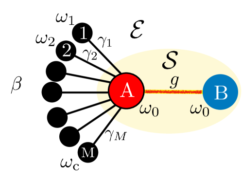
Figure 1: Schematic of the model: the composite system $\mathcal{S}$ is formed of two harmonic oscillators A and B of equal frequency $\omega_{0}$ which interact via an exchange Hamiltonian coupling characterized by the constant $g$. The subsystem A is also coupled with the modes $k\in\{1,2,\dots M\}$ of a thermal environment $\mathcal{E}$ at temperature $1/\beta$ (again the interaction is mediated by an exchange Hamiltonian with constants $\gamma_{k}$).

II The model

The model we consider is schematically described in Fig. 1. It consists into a bipartite system $\mathcal{S}$ composed of two resonant bosonic modes A and B of frequency $\omega_{0}$ and described by the ladder operators $a,a^{\dagger}$ and $b,b^{\dagger}$, that interact through an excitation preserving coupling characterized by an intensity parameter $g\geq 0$. Accordingly, setting $\hbar=1$, the free Hamiltonian of $\mathcal{S}$ reads

$$H_{\rm S}:=H_{\rm S,0}+H_{\rm S,g}\leavevmode\nobreak\ ,$$ (1)

$$H_{\rm S,0}:=\omega_{\rm A}a^{\dagger}a+\omega_{\rm B}b^{\dagger}b\leavevmode\nobreak\ ,{\rm\qquad with\qquad}\omega_{\rm A}=\omega_{\rm B}:=\omega_{0}\leavevmode\nobreak\ ,$$

$$H_{\rm S,g}:=g(a^{\dagger}b+{\rm h.c.})\leavevmode\nobreak\ ,$$

which can also be conveniently expressed as

$$H_{\rm S} = \omega_{+}\gamma_{+}^{\dagger}\gamma_{+}+\omega_{-}\gamma_{-}^{\dagger}\gamma_{-}\leavevmode\nobreak\ ,$$ (2)

with

$$\omega_{\pm} := \omega_{0}\pm g\leavevmode\nobreak\ \;,\qquad\gamma_{\pm}:=\frac{1}{\sqrt{2}}(a\pm b)\;,$$ (3)

being, respectively, the associated eigenmode frequencies and operators  emary2003chaos , the last obeying the commutation rules

$$\Big{[}\gamma_{-},\gamma_{+}\Big{]}_{-}=\Big{[}\gamma_{-},\gamma^{\dagger}_{+}\Big{]}_{-}=0\leavevmode\nobreak\ ,\leavevmode\nobreak\ \Big{[}\gamma_{\pm},\gamma^{\dagger}_{\pm}\Big{]}_{-}=1\leavevmode\nobreak\ .$$ (4)

Through the exclusive mediation of subsystem A, we then assume ${\cal S}$ to be connected with an external environment ${\cal E}$ formed of a collection of a large number $M$ of independent bosonic modes, no direct coupling being instead allowed between B and ${\cal E}$. Indicating with $c_{k},c_{k}^{\dagger}$ the ladder operators of the $k$-th mode of ${\cal E}$, we hence express the full Hamiltonian of the joint system $\mathcal{S}+\mathcal{E}$ as

$$H:=H_{\rm S}+H_{\rm E}+H_{1}\;,$$ (5)

with

$$H_{\rm E}:=\sum_{k=1}^{M}\omega_{k}c_{k}^{\dagger}c_{k}\leavevmode\nobreak\ ,\qquad H_{1}:=\sum_{k=1}^{M}\gamma_{k}(a^{\dagger}c_{k}+{\rm h.c.})\;,$$ (6)

being respectively the free Hamiltonian of the environment and the exchange coupling between A and ${\cal E}$. More in details, in our analysis we shall assume the frequencies $\omega_{k}$ of the environmental modes to be equally spaced with a cut-off value $\omega_{c}>\omega_{0}$, i.e.

$$\omega_{k}:=\frac{k}{M}\omega_{\rm c}\leavevmode\nobreak\ ,\hskip 56.9055ptk\in\{1,...,M\}\;,$$ (7)

and take the system-environment coupling constants $\gamma_{k}$ to have the form

$$\gamma_{k}:=\sqrt{\kappa(\omega_{0})\left(\frac{\omega_{k}}{\omega_{0}}\right)^{\alpha}\frac{\omega_{c}}{2\pi M}}\;,$$ (8)

with $\kappa(\omega_{0})$ controlling the effective strength of the interaction between A and ${\cal E}$. The parameter $\alpha\geq 0$ appearing in Eq. (8) gauges the bath’s dispersion relation by imposing the following form for the (rescaled) spectral density of the reservoirs modes hofer2017markovian

$$\kappa(\omega):=2\pi\sum_{k=1}^{M}\gamma_{k}^{2}\delta(\omega-\omega_{k})=\kappa(\omega_{0})\left(\frac{\omega}{\omega_{0}}\right)^{\alpha}\leavevmode\nobreak\ \Theta(\omega_{\rm c}-\omega)\;,$$ (9)

with $\Theta(x)$ being the Heaviside step function ($\alpha=1$, $\alpha>1$ and $\alpha<1$ being associated to the Ohmic, super-Ohmic, and sub-Ohmic scenarios respectively OHM ). Finally we shall assume the joint ${\cal S}+{\cal E}$ system to be initialized into a factorized state

$$\rho_{\rm SE}(0)=\rho_{\rm S}(0)\otimes\rho_{\rm E}(0)\;,$$ (10)

where the bath is in a thermal state of temperature $1/\beta>0$:

$$\rho_{\rm E}(0) := \frac{e^{-\beta H_{\rm E}}}{{\rm tr}[e^{-\beta H_{\rm E}}]}=\rho_{1}(\beta)\otimes\dots\otimes\rho_{M}(\beta)\leavevmode\nobreak\ ,$$ (11)

$$\rho_{k}(\beta) := \frac{e^{-\beta\omega_{k}c^{\dagger}_{k}c_{k}}}{{\rm tr}[e^{-\beta\omega_{k}c^{\dagger}_{k}c_{k}}]}\leavevmode\nobreak\ .$$ (12)

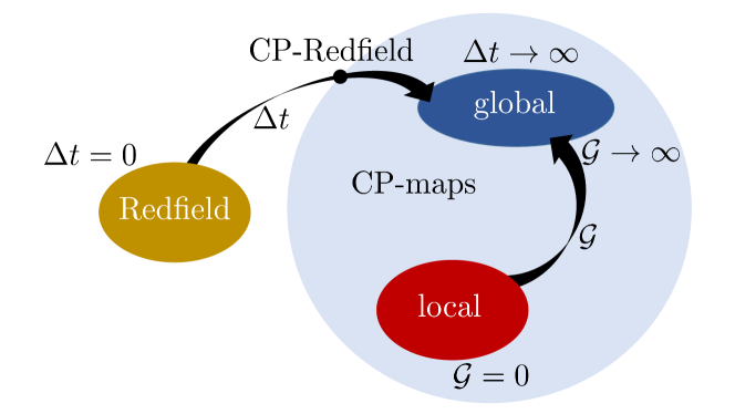
Figure 2: Schematic representation of the continuous transitions from the Redfield ME to the Global ME (25) passing through the coarse-grained Redfield MEs (13), and from the Local ME (28) to the Global ME using the time-dependent convex mixture (31). The dot indicates the completely positive map defined by the CP-Redfield ME obtained by saturating the bound in Eq. (23).

III Approximated equations for ${\cal S}$

In this section we review the different ME approaches one can use to effectively describe the evolution of the system ${\cal S}$ by integrating away the degrees of freedom of the environment ${\cal E}$. We shall start our presentation by introducing the coarse-grained regularized version of the Redfield equation farina2019psa , which includes the Global ME as a special case. We then introduce the local ME approach and finally discuss the phenomenological approach which employs convex combinations of local and global ME solutions. Since most of the derivations of the above expressions are discussed in details elsewhere (see e.g. breuer2002theory ) here we just give an overview of the methods involved and refer the interested reader to the Appendix A for further details.

III.1 From CP-Redfield ME to Global ME

The starting point of this section is the Redfield equation which one obtains by expressing the dynamical evolution of the joint system in the interaction picture, and enforcing the Born and, then, the Markov approximations breuer2002theory . The Born approximation assumes that the $\mathcal{S}+\mathcal{E}$ coupling is weak in such a way that the state of $\mathcal{E}$ is negligibly influenced by the presence of $\mathcal{S}$, while the Markov approximations assumes invariance of the interaction-picture system state over time-scales of order $\tau_{\rm E}$, the last being the time over which $\mathcal{E}$ loses the information coming from $\mathcal{S}$ and can be estimated from width of the bath correlation functions (see Appendix D).

As anticipated in the introductory section, the Redfield equation does not ensure completely positive evolutions and in certain cases neither positive evolution, hence preventing one from framing the obtained results with the probabilistic interpretation of quantum mechanics. To cure this issue we refer to the version of the partial secular approximation described in Ref. farina2019psa . Performing a coarse-grain averaging on the Redfield equation in interaction picture over a time interval $\Delta t$ that is much larger than the typical time scale of the system state in interaction picture, is a way to appropriately smooth the non-secular terms responsible of the non-positive character, even in a tight way. As schematically pictured in Fig. 2, by moving the parameter $\Delta t$ along the interval $[0,\infty[$ the reported technique is also capable to formally connect the original Redfield equation ($\Delta t=0$) and the full secular approximation ($\Delta t=\infty$) in a continuous way. Expressed in Schrödinger picture, the coarse-grained Redfield equation for the evolution of $\rho_{\rm S}$ for fixed coarse-graining time $\Delta t$, reads

$$\dot{\rho_{\rm S}}(t)=-i\Big{[}H_{\rm S}+H_{\rm LS}^{(\Delta t)},\rho_{\rm S}(t)\Big{]}_{-}$$ (13)

$$\qquad+\sum_{\sigma,\sigma^{\prime}=\pm}S_{\sigma\sigma^{\prime}}^{(\Delta t)}\Big{\{}\gamma^{(1)}_{\sigma\sigma^{\prime}}\Big{(}\gamma_{\sigma}^{\dagger}{\rho_{\rm S}}(t)\gamma_{\sigma^{\prime}}-\frac{1}{2}\Big{[}\gamma_{\sigma^{\prime}}\gamma_{\sigma}^{\dagger},{\rho_{\rm S}}(t)\Big{]}_{+}\Big{)}$$

$$\qquad\qquad+\gamma^{(2)}_{\sigma^{\prime}\sigma}\Big{(}\gamma_{\sigma^{\prime}}{\rho_{\rm S}}(t)\gamma_{\sigma}^{\dagger}-\frac{1}{2}\Big{[}\gamma_{\sigma}^{\dagger}\gamma_{\sigma^{\prime}},{\rho_{\rm S}}(t)\Big{]}_{+}\Big{)}\Big{\}},$$

where hereafter we shall use the symbols $\Big{[}\cdots,\cdots\Big{]}_{\mp}$ to represents commutator and anti-commutator relations, where $\gamma_{\pm}$ are the eigenmode operators of $H_{\rm S}$ introduced in Eq. (3), and where

$$H_{\rm LS}^{(\Delta t)}:=\sum_{\sigma,\sigma^{\prime}=\pm}S_{\sigma\sigma^{\prime}}^{(\Delta t)}(\eta_{\sigma\sigma^{\prime}}^{(1)}+\eta_{\sigma^{\prime}\sigma}^{(2)})\gamma^{\dagger}_{\sigma}\gamma_{\sigma^{\prime}}\leavevmode\nobreak\ ,$$ (14)

being the so called Lamb-shift Hamiltonian correction term. As indicated by the notation, the dependence of Eq. (13) upon the coarse-graining time interval $\Delta t$ is carried out by the tensor $S_{\sigma\sigma^{\prime}}^{(\Delta t)}$ of components

$$S_{\sigma\sigma^{\prime}}^{(\Delta t)} := {\rm sinc}\left(\tfrac{(\sigma-\sigma^{\prime})g\Delta t}{2}\right)$$

$$= \delta_{\sigma\sigma^{\prime}}+(1-\delta_{\sigma\sigma^{\prime}})\;{\rm sinc}(g\Delta t)\leavevmode\nobreak\ ,$$

with ${\rm sinc}(x):=\sin(x)/x$ being the cardinal sinus. The functional dependence of the right-hand-side of (13) upon the bath temperature is instead carried on by the tensors $\gamma^{(i)}_{\sigma\sigma^{\prime}}$ and $\eta^{(i)}_{\sigma\sigma^{\prime}}$. Specifically, for $\sigma,\sigma^{\prime}\in\{+,-\}$ and $i\in\{1,2\}$, these elements fulfill the constraints

$$\gamma^{(i)}_{\sigma\sigma^{\prime}}:=\frac{\gamma^{(i)}_{\sigma\sigma}+\gamma^{(i)}_{\sigma^{\prime}\sigma^{\prime}}}{2}+i(\eta^{(i)}_{\sigma\sigma}-\eta^{(i)}_{\sigma^{\prime}\sigma^{\prime}})\leavevmode\nobreak\ ,$$ (16)

$$\eta^{(i)}_{\sigma\sigma^{\prime}}:=-i\frac{\gamma^{(i)}_{\sigma\sigma}-\gamma^{(i)}_{\sigma^{\prime}\sigma^{\prime}}}{4}+\frac{\eta^{(i)}_{\sigma\sigma}+\eta^{(i)}_{\sigma^{\prime}\sigma^{\prime}}}{2}\leavevmode\nobreak\ ,$$ (17)

which allows one to express all of them in terms of their diagonal ($\sigma=\sigma^{\prime}$) components

$$\gamma_{\sigma\sigma}^{(1)} := \frac{1}{2}\leavevmode\nobreak\ \kappa(\omega_{\sigma})\leavevmode\nobreak\ \mathcal{N}(\omega_{\sigma})\leavevmode\nobreak\ ,$$ (18)

$$\gamma_{\sigma\sigma}^{(2)} := \frac{1}{2}\leavevmode\nobreak\ \kappa(\omega_{\sigma})\leavevmode\nobreak\ [1+\mathcal{N}(\omega_{\sigma})]\leavevmode\nobreak\ ,$$ (19)

$$\eta^{(1)}_{\sigma\sigma} := \frac{1}{2}\mathchoice{{\vbox{\hbox{$\textstyle-$}}\kern-4.86108pt}}{{\vbox{\hbox{$\scriptstyle-$}}\kern-3.25pt}}{{\vbox{\hbox{$\scriptscriptstyle-$}}\kern-2.29166pt}}{{\vbox{\hbox{$\scriptscriptstyle-$}}\kern-1.875pt}}\!\int_{0}^{\infty}d\epsilon\leavevmode\nobreak\ \frac{1}{2\pi}\frac{\kappa(\epsilon)\mathcal{N}(\epsilon)}{\epsilon-\omega_{\sigma}}\leavevmode\nobreak\ ,$$ (20)

$$\eta^{(2)}_{\sigma\sigma} := -\frac{1}{2}\mathchoice{{\vbox{\hbox{$\textstyle-$}}\kern-4.86108pt}}{{\vbox{\hbox{$\scriptstyle-$}}\kern-3.25pt}}{{\vbox{\hbox{$\scriptscriptstyle-$}}\kern-2.29166pt}}{{\vbox{\hbox{$\scriptscriptstyle-$}}\kern-1.875pt}}\!\int_{0}^{\infty}d\epsilon\leavevmode\nobreak\ \frac{1}{2\pi}\frac{\kappa(\epsilon)[1+\mathcal{N}(\epsilon)]}{\epsilon-\omega_{\sigma}}\;,$$ (21)

with $\kappa(\omega)$ the spectral density of the reservoirs defined in Eq. (9) and with

$$\mathcal{N}(\omega_{k}):=\mbox{Tr}[c_{k}^{\dagger}c_{k}\rho_{k}(\beta)]=\frac{1}{e^{\beta\omega_{k}}-1}\;,$$ (22)

being the Bose-Einstein factor of the mode $k$ of the thermal bath.

For $g\Delta t\rightarrow 0$, $S_{\sigma\sigma^{\prime}}^{(\Delta t)}$ assumes constant value $1$ for all $\sigma$ and $\sigma^{\prime}$: this corresponds to the pathological case of the (uncorrected) Redfield equation in which both the diagonal (secular) and the off-diagonal (non-secular) $\sigma,\sigma^{\prime}$ terms of the right-hand-side of Eq. (13) contribute at the same level to the dynamical evolution of $\rho_{\rm S}(t)$ paving the way to unwanted non-positive effects. As $g\Delta t$ increases the off-diagonal component $S_{+-}^{(\Delta t)}={\rm sinc}(g\Delta t)$ acts as the smoothing factor for the non-secular ($\sigma\neq\sigma^{\prime}$) part of the ME, which gets progressively depressed as the coarse-grain time interval $\Delta t$ gets comparable or even larger than the inverse of the energy scale $g$ of the system. Following Ref. farina2019psa one can then show that the model admits a (finite) threshold value for $\Delta t$ above which Eq. (13) acquires the explicit GKSL form that is necessary and sufficient to ensure complete positivity of the resulting evolution. Specifically, as discussed in details in Appendix B, such threshold is triggered by the inequality

$$|{S_{+-}^{(\Delta t)}}|\leq\min_{i\in\{1,2\}}\sqrt{\tfrac{\gamma_{++}^{(i)}\gamma_{--}^{(i)}}{\lvert\gamma_{+,-}^{(i)}\lvert^{2}}}\;.$$ (23)

In the following, the equation (13) at positivity threshold, i.e. with the choice of ${S_{+-}^{(\Delta t)}}$ tightly saturating the bound of Eq. (23), will be called CP-Redfield.

A numerical study of the condition (23) for some selected values of the system parameters is presented in Fig. 3.

\begin{overpic}[width=424.94574pt]{figs/pv1,oC3,g0,3__pos-th_Nb0__Nb0max_10.pdf}\end{overpic}

Figure 3: (Color online) Plot of the quantities in the right hand side of the inequality (23) for i=1 (black full line) and i=2 (red dashed line) as function of the bath temperature $1/\beta$ which we parametrize through $\mathcal{N}(\omega_{0})={1}/({e^{\beta\omega_{0}}-1})$. The blue region represents the values of $|{S_{+-}^{(\Delta t)}}|$ which satisfy the inequality (23) ensuring completely positive dynamics of the coarse-grain Redfield equation (13). We chose the parameters $g=0.3\omega_{0}$, $\omega_{c}=3\omega_{0}$, and $\alpha=1$ (Ohmic spectral density regime). Notice the logarithmic scale on the abscissa.

This plot makes it clear that the low temperature regime ($\mathcal{N}(\omega_{0})\ll 1$) constraints one to take very small values of $|{S_{+-}^{(\Delta t)}}|$ to guarantee the completely positive character of the evolution farina2019psa , while just a tiny correction is needed at high temperatures. These facts are in full agreement with the observation suarez1992memory ; cheng2005markovian ; ishizaki2009adequacy that the non-positivity character of the Redfield equation is enhanced at low temperature as a signature of the deviations from the Born-Markov assumptions underlying it hartmann2020accuracy . We stress that, in this context, non-positivity is originated by the multipartite nature of $\mathcal{S}$: indeed, as $g\rightarrow 0$, the right-hand side of Eq. (23) tends to 1 and consequently the non-positivity of the Redfield ME disappears in this limit. Notice finally that irrespectively from the value of $g$, Eq. (23) is trivially fulfilled in the asymptotic $g\Delta t\rightarrow\infty$ limit where $|{S_{+-}^{(\Delta t)}}|$ approaches the value zero leading to

$$S_{\sigma\sigma^{\prime}}^{(\infty)}=\delta_{\sigma\sigma^{\prime}}\;.$$ (24)

This condition identifies the full secular approximation of Eq. (13) that transforms such equation into the Global ME of the model which, for the sake of completeness, we report here in its explicit form

$$\dot{\rho}_{\rm S}(t)=-i\Big{[}H_{\rm S}+H_{\rm LS}^{\rm(glob)},\rho_{\rm S}(t)\Big{]}_{-}$$ (25)

$$\;+\sum_{\sigma=\pm}\Big{\{}\frac{1}{2}\kappa(\omega_{\sigma})\mathcal{N}(\omega_{\sigma})\Big{(}\gamma_{\sigma}^{\dagger}{\rho_{\rm S}}(t)\gamma_{\sigma}-\frac{1}{2}\Big{[}\gamma_{\sigma}\gamma_{\sigma}^{\dagger},{\rho_{\rm S}}(t)\Big{]}_{+}\Big{)}$$

$$\;+\frac{1}{2}\kappa(\omega_{\sigma})[1+\mathcal{N}(\omega_{\sigma})]\Big{(}\gamma_{\sigma}{\rho_{\rm S}}(t)\gamma_{\sigma}^{\dagger}-\frac{1}{2}\Big{[}\gamma_{\sigma}^{\dagger}\gamma_{\sigma},{\rho_{\rm S}}(t)\Big{]}_{+}\Big{)}\Big{\}}\leavevmode\nobreak\ ,$$

with

$$H_{\rm LS}^{\rm(glob)} := H_{\rm LS}^{(\infty)}=\sum_{\sigma=\pm}{\delta\omega_{\sigma}}\gamma^{\dagger}_{\sigma}\gamma_{\sigma}\,,$$ (26)

$${\delta\omega_{\sigma}} := \eta_{\sigma\sigma}^{(1)}+\eta_{\sigma\sigma}^{(2)}=\frac{1}{4\pi}\mathchoice{{\vbox{\hbox{$\textstyle-$}}\kern-4.86108pt}}{{\vbox{\hbox{$\scriptstyle-$}}\kern-3.25pt}}{{\vbox{\hbox{$\scriptscriptstyle-$}}\kern-2.29166pt}}{{\vbox{\hbox{$\scriptscriptstyle-$}}\kern-1.875pt}}\!\int_{0}^{\infty}d\epsilon\frac{\kappa(\epsilon)}{\omega_{\sigma}-\epsilon},$$ (27)

being the secular component of the Lamb-shift term hofer2017markovian .

III.2 Local ME

The Local ME for ${\cal S}$ is a GKSL equation characterized by Lindblad operators which act locally on the mode A. Explicitly it is given by

$$\dot{\rho_{\rm S}}(t)=-i\Big{[}H_{\rm S}+H_{\rm LS}^{\rm(loc)},\rho_{\rm S}(t)\Big{]}_{-}$$ (28)

$$\qquad+\kappa(\omega_{0})\mathcal{N}(\omega_{0})\Big{(}a^{\dagger}\rho_{\rm S}(t)a-\frac{1}{2}\Big{[}aa^{\dagger},\rho_{\rm S}(t)\Big{]}_{+}\Big{)}$$

$$\qquad+\kappa(\omega_{0})(1+\mathcal{N}(\omega_{0}))\Big{(}a\rho_{\rm S}(t)a^{\dagger}-\frac{1}{2}\Big{[}a^{\dagger}a,\rho_{\rm S}(t)\Big{]}_{+}\Big{)}\;,$$

with $\kappa(\omega_{0})$ and $\mathcal{N}(\omega_{0})$ defined as in the previous section and where now the Lamb-shift term is expressed as a modification of the local Hamiltonian of the A mode only, i.e.

$$H_{\rm LS}^{\rm(loc)} := \delta\omega_{\rm A}\leavevmode\nobreak\ a^{\dagger}a\,,$$ (29)

$$\delta\omega_{\rm A} := \frac{1}{2\pi}\mathchoice{{\vbox{\hbox{$\textstyle-$}}\kern-4.86108pt}}{{\vbox{\hbox{$\scriptstyle-$}}\kern-3.25pt}}{{\vbox{\hbox{$\scriptscriptstyle-$}}\kern-2.29166pt}}{{\vbox{\hbox{$\scriptscriptstyle-$}}\kern-1.875pt}}\!\int_{0}^{\infty}d\omega\frac{\kappa(\omega)}{\omega_{0}-\omega}.$$ (30)

Effectively Eq. (28) can be obtained starting from a Hamiltonian model for the global system ${\cal S}+{\cal E}$ where one initially completely neglects the presence of the B mode, enforces the same approximations that leads one to (25) (i.e. the Born, Markov, and full secular approximation), and finally introduces B and its coupling with A as an additive Hamiltonian contribution in the resulting expression. More formally as shown e.g. in Ref. hofer2017markovian , Eq. (28) can be derived in the weak internal coupling limit $g\tau_{\rm E}\ll 1$ ($\tau_{\rm E}$ being the bath memory time scale, see Appendix D for details) which allows one to treat the interaction between A and B as a perturbative correction with respect to the direct A-${\cal E}$ coupling – see Appendix A for more on this.

III.3 Convex mixing of Local and Global solutions

As we shall explicitly see in the next section (see Eq. (39)), the main advantage offered by the Global ME (25) is that it provides an accurate description of the steady state of ${\cal S}$ at least in the infinitesimally small ${\cal S}+{\cal E}$ coupling regime where on pure thermodynamic considerations one expects independent thermalization of the eigenmodes $\gamma_{\pm}$ of the system. On the contrary the steady state predicted by the Local ME (28) is wrong (even if increasingly accurate as $g/\omega_{0}\rightarrow 0$) because it implies the thermalization of the subsystems A and B regardless of the presence of the internal coupling $H_{\rm S,g}$. Conversely, the Local ME has the quality to predict Rabi oscillations between A and B at shorter time scales, that are completely neglected when adopting the Global ME.

In view of these observations a reasonable way of keeping local effects during the transient still maintaining an accurate steady state solution is to adopt an appropriate phenomenological ansatz describing the evolution of ${\cal S}$ in terms of quantum trajectories that interpolate between the solutions $\rho^{(\rm glob)}_{\rm S}(t)$ and $\rho^{(\rm loc)}_{\rm S}(t)$ of the Global and Local ME, see Fig. 2. The simplest of these construction is provided by the following time-dependent mixture

$$\rho^{(\rm mix)}_{\rm S}(t):=e^{-\mathcal{G}t}\rho^{(\rm loc)}_{\rm S}(t)+\left(1-e^{-\mathcal{G}t}\right)\rho^{(\rm glob)}_{\rm S}(t)\;.$$ (31)

In this expression $\mathcal{G}>0$ is an effective rate, whose inverse fix the time scale of the problem that determines when global thermalization effect start dominating the system dynamics. Accordingly Eq. (31) allows us to keep local effects for short time scales $t\lesssim\mathcal{G}^{-1}$ and the correct thermalization of the eigenmodes of the system at longer time scales $t\gg\mathcal{G}^{-1}$. The above formula can be interpreted as follows: the environment needs a finite amount of time to become aware of the presence of the part B because of its short time correlations (Markovian hypothesis). The specific value of $\mathcal{G}$ is a free variable in this model and works as a fitting parameter: its value can be even estimated quite roughly because of the relatively large time interval at intermediate time scales where the Global and Local approximations look alike (more on this later). It is finally worth observing that from the complete positivity properties of both the solutions of the Global and Local ME, it follows that (31) also fulfills such requirement (indeed convex combinations of completely positive transformations are also completely positive). On the contrary at variance with the original expressions (25) and (28), as well as the CP-Redfield expression (13), Eq. (31) will typically exhibit a non Markovian character and will not be possible to present it in the form of a GKSL differential equation. This property is a direct consequence of the fact that the set of Markovian evolutions is not closed under convex combinations  CONVEX .

IV Dynamics

In the study of the approximated equations introduced in the previous section, as well as for their comparison with the exact solution of the ${\cal S}+{\cal E}$ dynamics, an important simplification arises from the choice we made in fixing the initial condition of ${\cal E}$. Indeed thanks to Eqs. (11), (12) the resulting CP-Redfield, Global, and Local MEs, happen to be Gaussian processes serafini2017quantum which admit complete characterization only in terms of the first and second moments of the field operators $\gamma_{\pm}$ (notice that while the mixture (31) does not fit into the set of Gaussian processes – formally speaking it belongs to the convex-hull of such set – we can still resort to the above simplification by exploiting the fact that $\rho^{(\rm mix)}_{\rm S}(t)$ is explicitly given by the sum of the Global and Local ME solutions). Accordingly in studying the dynamics of our approximated schemes we can just focus on the functions $\langle\gamma_{\sigma}\rangle(t):=\mbox{Tr}[\gamma_{\sigma}\rho_{\rm S}(t)]$, $\langle\gamma_{\sigma}\gamma_{\sigma^{\prime}}\rangle(t):=\mbox{Tr}[\gamma_{\sigma}\gamma_{\sigma^{\prime}}\rho_{\rm S}(t)]$, and $\langle\gamma_{\sigma}^{{\dagger}}\gamma_{\sigma^{\prime}}\rangle(t):=\mbox{Tr}[\gamma_{\sigma}^{{\dagger}}\gamma_{\sigma^{\prime}}\rho_{\rm S}(t)]$ whose temporal dependence can be determined by solving a restricted set of coupled linear differential equations. We also observe that since the full Hamiltonian (5) conserves the total number of excitations in the ${\cal S}+{\cal E}$ model, coupling between excitations conserving and non-conserving moments are prevented cattaneo2019simmetry yielding further simplification in the analysis.

Having clarified these points, in what follows we shall focus on the special case where the input state of ${\cal S}$ is fixed assuming that both A and B are initialized in the ground states of their local Hamiltonians, i.e.

$$\rho_{\rm S}(0) = \ket{0}_{\rm A}\bra{0}\otimes\ket{0}_{\rm B}\bra{0}\leavevmode\nobreak\ ,$$ (32)

with $|{0}\rangle$ representing the zero Fock state of the corresponding mode. Under these conditions the input state is Gaussian serafini2017quantum and, evolved under CP-Redfield, Global, Local and the exact dynamics, will remain Gaussian at all time. Furthermore all the first order moments and all the non-excitation-conserving second order terms exactly nullify, i.e.

$$\langle\gamma_{\sigma}\rangle(t)=0\;,\qquad\langle\gamma_{\sigma}\gamma_{\sigma^{\prime}}\rangle(t)=0\;,$$ (33)

leaving only a restricted set of equations to be explicitly integrated. In particular, for the case of the coarse-grained Redfield equation (13) we get

$$\frac{d}{dt}\langle\gamma_{+}^{\dagger}\gamma_{+}\rangle(t) = -\frac{1}{2}\kappa(\omega_{+})[\langle\gamma_{+}^{\dagger}\gamma_{+}\rangle(t)-\mathcal{N}(\omega_{+})]$$

$$+\;S_{+-}^{(\Delta t)}\times\left\{2\leavevmode\nobreak\ {\rm Im}\left((\eta^{(1)}_{+-}+\eta^{(2)}_{-+})\langle\gamma_{-}\gamma_{+}^{\dagger}\rangle(t)\right)+{\rm Re}\left[(\gamma^{(1)}_{+-}-\gamma^{(2)}_{-+})\langle\gamma_{-}\gamma_{+}^{\dagger}\rangle(t)\right]\right\}\leavevmode\nobreak\ ,$$

$$\frac{d}{dt}\langle\gamma_{-}^{\dagger}\gamma_{-}\rangle(t) = -\frac{1}{2}\kappa(\omega_{-})[\langle\gamma_{-}^{\dagger}\gamma_{-}\rangle(t)-\mathcal{N}(\omega_{-})]$$

$$+\;S_{+-}^{(\Delta t)}\times\left\{-2\leavevmode\nobreak\ {\rm Im}\left((\eta^{(1)}_{+-}+\eta^{(2)}_{-+})\langle\gamma_{-}\gamma_{+}^{\dagger}\rangle(t)\right)+{\rm Re}\left[(\gamma^{(1)}_{+-}-\gamma^{(2)}_{-+})\langle\gamma_{-}\gamma_{+}^{\dagger}\rangle(t)\right]\right\}\leavevmode\nobreak\ ,$$

$$\frac{d}{dt}\langle\gamma_{-}\gamma_{+}^{\dagger}\rangle(t) = \{i(\omega_{+}+\delta\omega_{+}-\omega_{-}-\delta\omega_{-})-\frac{1}{4}[\kappa(\omega_{+})+\kappa(\omega_{-})]\}\langle\gamma_{-}\gamma_{+}^{\dagger}\rangle(t)$$

$$+\;S_{+-}^{(\Delta t)}\times\left\{i(\eta^{(1)}_{-+}+\eta^{(2)}_{+-})\left[\langle\gamma_{-}^{\dagger}\gamma_{-}\rangle(t)-\langle\gamma_{+}^{\dagger}\gamma_{+}\rangle(t)\right]+\gamma^{(1)}_{-+}+\frac{1}{2}(\gamma^{(1)}_{-+}-\gamma^{(2)}_{+-})\left[\langle\gamma_{-}^{\dagger}\gamma_{-}\rangle(t)+\langle\gamma_{+}^{\dagger}\gamma_{+}\rangle(t)\right]\right\}\leavevmode\nobreak\ ,$$

with initial values

$$\langle\gamma_{+}^{\dagger}\gamma_{+}\rangle(0) = \langle\gamma_{-}^{\dagger}\gamma_{-}\rangle(0)=\langle\gamma_{-}\gamma_{+}^{\dagger}\rangle(0)=0\leavevmode\nobreak\ ,$$ (35)

imposed by (32). In particular in the case of full secular approximation ($S_{+-}^{(\Delta t)}=0$) the above set of equations become

$$\frac{d}{dt}\langle\gamma_{+}^{\dagger}\gamma_{+}\rangle(t) = -\frac{1}{2}\kappa(\omega_{+})[\langle\gamma_{+}^{\dagger}\gamma_{+}\rangle(t)-\mathcal{N}(\omega_{+})]\;,$$ (36)

$$\frac{d}{dt}\langle\gamma_{-}^{\dagger}\gamma_{-}\rangle(t) = -\frac{1}{2}\kappa(\omega_{-})[\langle\gamma_{-}^{\dagger}\gamma_{-}\rangle(t)-\mathcal{N}(\omega_{-})]\;,$$

$$\frac{d}{dt}\langle\gamma_{-}\gamma_{+}^{\dagger}\rangle(t) = \{i(\omega_{+}+\delta\omega_{+}-\omega_{-}-\delta\omega_{-})$$

$$-\frac{1}{4}[\kappa(\omega_{+})+\kappa(\omega_{-})]\}\langle\gamma_{-}\gamma_{+}^{\dagger}\rangle(t)\;,$$

which yield the evolution of the moments for the Global ME (25). Similar considerations hold true for the Local ME (28). In this case following Refs. hofer2017markovian ; farina2019charger we get

$$\frac{d}{dt}\langle\gamma_{+}^{\dagger}\gamma_{+}\rangle(t) = -\frac{1}{2}\kappa(\omega_{0})[\langle\gamma_{+}^{\dagger}\gamma_{+}\rangle(t)-\mathcal{N}(\omega_{0})+{\rm Re}\langle\gamma_{-}\gamma_{+}^{\dagger}\rangle(t)]+\delta\omega_{\rm A}\leavevmode\nobreak\ {\rm Im}\langle\gamma_{-}\gamma_{+}^{\dagger}\rangle(t)\leavevmode\nobreak\ ,$$ (37)

$$\frac{d}{dt}\langle\gamma_{-}^{\dagger}\gamma_{-}\rangle(t) = -\frac{1}{2}\kappa(\omega_{0})[\langle\gamma_{-}^{\dagger}\gamma_{-}\rangle(t)-\mathcal{N}(\omega_{0})+{\rm Re}\langle\gamma_{-}\gamma_{+}^{\dagger}\rangle(t)]-\delta\omega_{\rm A}\leavevmode\nobreak\ {\rm Im}\langle\gamma_{-}\gamma_{+}^{\dagger}\rangle(t)\leavevmode\nobreak\ ,$$

$$\frac{d}{dt}\langle\gamma_{-}\gamma_{+}^{\dagger}\rangle(t) = [i2g-\frac{1}{2}\kappa(\omega_{0})]\langle\gamma_{-}\gamma_{+}^{\dagger}\rangle(t)+\frac{\kappa(\omega_{0})}{2}\{\mathcal{N}(\omega_{0})-\frac{1}{2}[\langle\gamma_{+}^{\dagger}\gamma_{+}\rangle(t)+\langle\gamma_{-}^{\dagger}\gamma_{-}\rangle(t)]\}+i\leavevmode\nobreak\ \frac{\delta\omega_{\rm A}}{2}[\langle\gamma_{-}^{\dagger}\gamma_{-}\rangle(t)-\langle\gamma_{+}^{\dagger}\gamma_{+}\rangle(t)]\leavevmode\nobreak\ ,$$

which, for a direct comparison with Eq. (36), we express here in terms of the eigenmodes $\gamma_{\pm}$.

IV.1 Evolution of the second moments

\begin{overpic}[width=173.44534pt]{figs/legend}\put(30.0,73.0){}\end{overpic}

\begin{overpic}[width=173.44534pt]{figs/moms-glob-30}\put(30.0,73.0){(a)}\end{overpic}

\begin{overpic}[width=173.44534pt]{figs/moms-glob-350}\put(30.0,73.0){}\put(-8.0,75.0){global}\end{overpic}

\begin{overpic}[width=173.44534pt]{figs/moms-loc-30}\put(30.0,73.0){(b)}\end{overpic}

\begin{overpic}[width=173.44534pt]{figs/moms-loc-350}\put(30.0,73.0){}\put(-8.0,75.0){local}\end{overpic}

\begin{overpic}[width=173.44534pt]{figs/moms-mix-30}\put(30.0,73.0){(c)}\end{overpic}

\begin{overpic}[width=173.44534pt]{figs/moms-mix-350}\put(30.0,73.0){}\put(-25.0,75.0){convex mixture}\end{overpic}

Figure 4: (Color online) Second order moments evaluated using the Global ME (a), the local ME (b), the convex mixture of Eq. (31) with $\mathcal{G}=0.4\kappa(\omega_{0})$ (c), compared with the ones predicted by the exact dynamics. As indicated by the legend continuous lines in the plots represent the quantities computed by solving the exact ${\cal S}+{\cal E}$ Hamiltonian model (5); dotted and dashed lines instead refer to the approximated solutions associated with Global, Local and Mixed approaches. Each panel contains two plots corresponding each to shorter (left) and longer (right) time scales. As clear from the right plot of panel (a), the Global ME approach provides a pretty good agreement with the exact solutions at large time scales, while fails in the short time domain. Exactly the opposite occurs for the Local ME approach presented in panel (b): here a good agreement with the exact solutions is found in the short time domain (left plot), while differences arise in the large time domain (right plot). The convex mixture approach (IV.1) finally appears to be able to maintain a good agreement with the exact results at times. In all the plots we used $\mathcal{N}(\omega_{0})=10$ (corresponding to $1/\beta\approx 10.5\omega_{0}$), $g=0.3\omega_{0}$, $\kappa(\omega_{0})=0.04\omega_{0}$, $\omega_{c}=3\omega_{0}$, $\alpha=1$.

A closer look at Eq. (36) reveals that in this case one has that for large enough $t$ we get

$$\langle\gamma^{\dagger}_{\rm\pm}\gamma_{\rm\pm}\rangle\Big{|}_{(\rm glob)}(\infty)=\mathcal{N(\omega_{\pm})}\;,\qquad\langle\gamma_{\rm-}\gamma^{\dagger}_{\rm+}\rangle\Big{|}_{(\rm glob)}(\infty)=0\;.$$ (38)

This enlightens the fact that, as anticipated at the beginning of Sec. III.3, the Global ME (25) imposes ${\cal S}$ to asymptotically converge toward the Gibbs thermal state

$$\rho^{(\rm glob)}_{\rm S}(\infty):=\frac{e^{-\beta H_{\rm S}}}{{\rm tr}[e^{-\beta H_{\rm S}}]}\;,$$ (39)

in agreement with what one would expect from purely thermodynamics considerations under weak-coupling conditions for the system-environment interactions. On the contrary the steady state predicted by the Local ME is wrong (even if increasingly accurate as $g/\omega_{0}\rightarrow 0$) because it implies the thermalization of the subsystems A and B regardless of the presence of the internal coupling $H_{\rm S,g}$. Indeed from Eq. (37) we get

$$\langle\gamma_{\pm}^{\dagger}\gamma_{\pm}\rangle\Big{|}_{(\rm loc)}(\infty)=\mathcal{N}(\omega_{0})\leavevmode\nobreak\ ,\qquad\langle\gamma_{-}\gamma_{+}^{\dagger}\rangle\Big{|}_{(\rm loc)}(\infty)=0$$ (40)

or equivalently

$$\langle a^{\dagger}a\rangle\Big{|}_{(\rm loc)}(\infty) = \langle b^{\dagger}b\rangle\Big{|}_{(\rm loc)}(\infty)=\mathcal{N}(\omega_{0})\leavevmode\nobreak\ ,$$ (41)

$$\langle ab^{\dagger}\rangle\Big{|}_{(\rm loc)}(\infty) = 0\;,$$ (42)

which identifies

$$\rho^{(\rm loc)}_{\rm S}(\infty):=\frac{e^{-\beta H_{\rm S,0}}}{{\rm tr}[e^{-\beta H_{\rm S,0}}]}\;,$$ (43)

as the new fixed point for the dynamical evolution (see also Appendix E). The discrepancy between the above expressions and Eqs. (38), (39) is even accentuated in the low temperature regime $\beta\omega_{0}\gg 1$, where in particular the ratio $\mathcal{N}(\omega_{-})/\mathcal{N}(\omega_{0})\simeq e^{\beta g}$ explodes exponentially.

The situation gets reversed at shorter time scales. Here the Local ME correctly presents coherent energy exchanges between A and B which instead the Global approach completely neglects. Indeed from Eq. (36) it follows that the Global ME predicts ${\rm Im}[\langle ab^{\dagger}\rangle(t)]=0$, the term being responsible of the Rabi oscillations between A and B. The Local ME on the contrary – when the Lamb-shift correction can be neglected – gives ${\rm Re}[\langle ab^{\dagger}\rangle(t)]=0$, the latter being proportional to the average internal interaction energy $\langle H_{\rm S,g}\rangle$.

The above observations are confirmed by the numerical study we present in the remaining of the section (see however also the material presented in Appendix E). In particular, in panels (a) and (b) of Fig. 4 the temporal evolution of the second order moments obtained by solving Eq. (36) and (37) are compared with the exact values of the corresponding quantities obtained by numerical integration of the exact ${\cal S}+{\cal E}$ Hamiltonian model along the lines detailed in Appendix D. In panel (c) of such figure we also present the results obtained by using the effective model of Sec. III.3, where according to Eq. (31) the expectation values of the relevant quantities are computed as

$$\langle\gamma_{\sigma}^{{\dagger}}\gamma_{\sigma^{\prime}}\rangle\Big{|}_{(\rm mix)}(t) = e^{-\mathcal{G}t}\langle\gamma_{\sigma}^{{\dagger}}\gamma_{\sigma^{\prime}}\rangle\Big{|}_{(\rm loc)}(t)$$

$$+\left(1-e^{-\mathcal{G}t}\right)\langle\gamma_{\sigma}^{{\dagger}}\gamma_{\sigma^{\prime}}\rangle\Big{|}_{(\rm glob)}(t)\;,$$

with $\langle\gamma_{\sigma}^{{\dagger}}\gamma_{\sigma^{\prime}}\rangle\Big{|}_{(\rm loc)}(t)$ and $\langle\gamma_{\sigma}^{{\dagger}}\gamma_{\sigma^{\prime}}\rangle\Big{|}_{(\rm glob)}(t)$ representing the solutions of Eq. (37) and Eq. (36) respectively. In our analysis the system parameters have been set in order to enforce ${\cal S}+{\cal E}$ weak-coupling conditions ($\omega_{0},\omega_{\pm}\gg\kappa(\omega_{0})$) to make sure that that the long term prediction (39) of the Global ME provides a proper description of the system dynamics. By the same token, the temperature of the bath has been fixed to be relatively high, i.e. $1/\beta\approx 10.5\omega_{0}$, to avoid to enhance correlation effects between the bath and the system which are not included in the Born and Markov approximations needed to derive both the Global and the Local ME hovhannisyan2020charging (a study of the impact of low temperature effects on the ${\cal S}+{\cal E}$ correlations is presented in Appendix D.2). Finally regarding the value of the phenomenological parameter ${\cal G}$ entering in (IV.1) we set it be equal to $0.4\kappa(\omega_{0})$ finding a relatively good agreement with the exact data at all times.

\begin{overpic}[width=212.47617pt]{figs/legend}\put(30.0,73.0){}\end{overpic}

\begin{overpic}[width=212.47617pt]{figs/moms-Rth-30}\put(30.0,73.0){(a)}\end{overpic}

\begin{overpic}[width=212.47617pt]{figs/moms-Rth-350}\put(30.0,73.0){} \put(-20.0,75.0){CP-Redfield} \end{overpic}

\begin{overpic}[width=212.47617pt]{figs/moms-R-30}\put(30.0,73.0){(b)}\end{overpic}

\begin{overpic}[width=212.47617pt]{figs/moms-R-350}\put(30.0,73.0){}\put(-15.0,75.0){Redfield} \end{overpic}

Figure 5: (Color online) Comparison between second order moments evaluated using the CP-Redfield (a) and Redfield (b) with the ones predicted by the exact dynamics. As in the case of Fig. 4 continuous lines represent the quantities computed by solving the exact ${\cal S}+{\cal E}$ Hamiltonian model (5) while dotted and dashed lines instead refer to the approximated solutions. Also each panel contains two plots corresponding each to shorter (left) and longer (right) time scales. In all the plots we used $\mathcal{N}(\omega_{0})=10$ (corresponding to $1/\beta\approx 10.5\omega_{0}$), $g=0.3\omega_{0}$, $\kappa(\omega_{0})=0.04\omega_{0}$, $\omega_{c}=3\omega_{0}$, $\alpha=1$ – same as those used in Fig. 4. The value of $\Delta t$ used to define CP-Redfield is such that ${S}^{(\Delta t)}_{+-}=0.989\leavevmode\nobreak\ ,$ which ensures the saturation of the inequality (23).

The convex combination (31) is not the only way of keeping the best from both the local and the global approximations. Indeed, by making a step back, one can consider the coarse-grained Redfield equations (IV) once that the pathology related to their non-positivity has been cured. A detailed study of the performances of this approach is presented in Fig. 5. Here, for the same values of the parameters used in Fig. 4, in panel (a) we exhibit the plots associated with the CP-Redfield equation obtained by fixing ${S_{+-}^{(\Delta t)}}$ in such a way to saturate the positivity bound (23), i.e. ${S}^{(\Delta t)}_{+-}=0.989$. As in the case of panel (c) of Fig. 5, we notice that CP-Redfield is in a good agreement with the exact data both at long and short time scales. As a check in panel (b) of Fig. 5 we also present the (uncorrected) Redfield equation obtained by setting in Eq. (IV) $\Delta t=0$, corresponding to have ${S_{+-}^{(\Delta t)}}=1$ which for the system parameters we choose gives a clear violation of the positivity bound (23). Interestingly enough, despite the fact that the resulting equation does not guarantee complete positivity of the associated evolution, we notice that also in this case one has an apparent good agreement with the exact results for all times.

\begin{overpic}[width=424.94574pt]{figs/gap1}\end{overpic}

Figure 6: (Color online) Plot of the local excitation gap $\langle a^{\dagger}a\rangle(t)-\langle b^{\dagger}b\rangle(t)$ for the different approximation methods and for the exact dynamics. Global ME (blue dashed line), Local ME (red dotted line), and convex Mixture approach (cyan dot-dashed-dashed line) predict an asymptotically zero value for such quantities. On the contrary Redfield (green dot-dashed line) and CP-Redfield (black dot-dot-dashed line) give an asymptotic final value for such quantity in agreement with the exact dynamics (magenta full and thicker line). In all the plots we used $\mathcal{N}(\omega_{0})=10$ (corresponding to $1/\beta\approx 10.5\omega_{0}$), $g=0.3\omega_{0}$, $\kappa(\omega_{0})=0.04\omega_{0}$, $\omega_{c}=3\omega_{0}$, $\alpha=1$ – same as those used in Figs. 4, 5. The value of $\Delta t$ used to define CP-Redfield is such that ${S}^{(\Delta t)}_{+-}=0.989\leavevmode\nobreak\ ,$ which ensures the saturation of the inequality (23).

In particular both CP-Redfield and Redfield equations appear to be able to capture a non-weak coupling correction to the asymptotic value of $2{\rm Re}\langle\gamma_{-}\gamma_{+}^{\dagger}\rangle(t)=\langle a^{\dagger}a\rangle(t)-\langle b^{\dagger}b\rangle(t)\leavevmode\nobreak\ ,$ an effect that is present in the exact model due to the fact that the subsystem A remains slightly correlated with the bath degrees of freedom, but which is not present when adopting neither Global, Local, or Mixed approximations (see Fig. 6). An evidence of this can be obtained by observing that from Eq. (IV) we have

$$2{\rm Re}\langle\gamma_{-}\gamma_{+}^{\dagger}\rangle(\infty)=\tfrac{S_{+-}^{(\Delta t)}}{\omega_{+}-\omega_{-}}$$

$$\times\mathchoice{{\vbox{\hbox{$\textstyle-$}}\kern-4.86108pt}}{{\vbox{\hbox{$\scriptstyle-$}}\kern-3.25pt}}{{\vbox{\hbox{$\scriptscriptstyle-$}}\kern-2.29166pt}}{{\vbox{\hbox{$\scriptscriptstyle-$}}\kern-1.875pt}}\!\int_{0}^{\infty}d\epsilon\leavevmode\nobreak\ \frac{\kappa(\epsilon)}{2\pi}\leavevmode\nobreak\ \left({\tfrac{\mathcal{N}(\epsilon)-\mathcal{N}(\omega_{+})}{\epsilon-\omega_{+}}-\tfrac{\mathcal{N}(\epsilon)-\mathcal{N}(\omega_{-})}{\epsilon-\omega_{-}}}\right)+O[\kappa(\omega_{0})^{2}]$$

which is exactly null for the Global ME ($S_{+-}^{(\Delta t)}=0$), but which is different from zero (and in good agreement with the exact result) both for the uncorrected Redfield equation ($S_{+-}^{(\Delta t)}=1$) and CP-Redfield (${S}^{(\Delta t)}_{+-}=0.989$).

\begin{overpic}[width=212.47617pt]{figs/avalc_1.pdf}\put(5.0,75.0){(a)}\end{overpic}

\begin{overpic}[width=212.47617pt]{figs/avalc_3.pdf}\put(5.0,75.0){(b)}\end{overpic}

Figure 7: (Color online) Plots of the quantity $\lambda_{\rm c}(t)$ of Eq. (46) for different approximation methods and using the exact result, at shorter (a) and longer (b) time scales. In all the plots we used $\mathcal{N}(\omega_{0})=10$ (corresponding to $1/\beta\approx 10.5\omega_{0}$), $g=0.3\omega_{0}$, $\kappa(\omega_{0})=0.04\omega_{0}$, $\omega_{c}=3\omega_{0}$, $\alpha=1$ – same as those used in Figs. 4-6. The value of $\Delta t$ used to define CP-Redfield is such that ${S}^{(\Delta t)}_{+-}=0.989\leavevmode\nobreak\ ,$ which saturates the inequality (23).

Despite the apparent success of the uncorrected Redfield equation reported above, a clear signature of its non-positivity can still be spotted by looking at a special functional of the second order moments of the model, i.e. the quantity

$$\lambda_{c}(t):=\frac{1}{2}{\rm min\{\leavevmode\nobreak\ eigenvalues}[\Gamma_{\rm S}(t)+i\Xi_{\rm S}]\leavevmode\nobreak\ \}\leavevmode\nobreak\ .$$ (46)

In the above definition $\Gamma_{\rm S}(t)$ and $\Xi_{\rm S}$ are respectively the covariance matrix and the symplectic form of the two-mode system ${\cal S}$. Expressed in terms of the eigenoperators $\gamma_{\pm}$ their elements are given by

$$[{\Gamma}_{\rm S}(t)]_{ij}:=\left\langle\Big{[}\boldsymbol{\Gamma}_{i}-\langle\boldsymbol{\Gamma}_{i}\rangle(t),\boldsymbol{\Gamma}_{j}^{\dagger}-\langle\boldsymbol{\Gamma}^{\dagger}_{j}\rangle(t)\Big{]}_{+}\right\rangle(t),$$ (47)

and

$$[\Xi_{\rm S}]_{ij}:=-i\left\langle\Big{[}\boldsymbol{\Gamma}_{i},\boldsymbol{\Gamma}_{j}^{\dagger}\Big{]}_{-}\right\rangle(t)=-i\begin{pmatrix}1&0&0&0\\ 0&-1&0&0\\ 0&0&1&0\\ 0&0&0&-1\end{pmatrix},$$ (48)

with $\boldsymbol{\Gamma}_{i}$ being the $i$-th component of the operator vector $\boldsymbol{\Gamma}:=(\gamma_{+},\gamma_{+}^{\dagger},\gamma_{-},\gamma_{-}^{\dagger})^{T}$. In particular due to the choice of the input state we made in Eq. (32), we get

$$\Gamma_{\rm S}(t)=\begin{pmatrix}2\langle\gamma_{+}^{\dagger}\gamma_{+}\rangle(t)+1&0&2\langle\gamma_{-}\gamma_{+}^{\dagger}\rangle(t)^{*}&0\\ 0&2\langle\gamma_{+}^{\dagger}\gamma_{+}\rangle(t)+1&0&2\langle\gamma_{-}\gamma_{+}^{\dagger}\rangle(t)\\ 2\langle\gamma_{-}\gamma_{+}^{\dagger}\rangle(t)&0&2\langle\gamma_{-}^{\dagger}\gamma_{-}\rangle(t)+1&0\\ 0&2\langle\gamma_{-}\gamma_{+}^{\dagger}\rangle(t)^{*}&0&2\langle\gamma_{-}^{\dagger}\gamma_{-}\rangle(t)+1\end{pmatrix}\leavevmode\nobreak\ ,$$ (49)

and hence

$$\frac{\Gamma_{\rm S}(t)+i\Xi_{\rm S}}{2}=\begin{pmatrix}\langle\gamma_{+}^{\dagger}\gamma_{+}\rangle(t)+1&0&\langle\gamma_{-}\gamma_{+}^{\dagger}\rangle(t)^{*}&0\\ 0&\langle\gamma_{+}^{\dagger}\gamma_{+}\rangle(t)&0&\langle\gamma_{-}\gamma_{+}^{\dagger}\rangle(t)\\ \langle\gamma_{-}\gamma_{+}^{\dagger}\rangle(t)&0&\langle\gamma_{-}^{\dagger}\gamma_{-}\rangle(t)+1&0\\ 0&\langle\gamma_{-}\gamma_{+}^{\dagger}\rangle(t)^{*}&0&\langle\gamma_{-}^{\dagger}\gamma_{-}\rangle(t)\end{pmatrix}\leavevmode\nobreak\ ,$$ (50)

$$\lambda_{c}(t)=\frac{1}{2}\{\langle\gamma_{+}^{\dagger}\gamma_{+}\rangle(t)+\langle\gamma_{-}^{\dagger}\gamma_{-}\rangle(t)-\sqrt{[\langle\gamma_{+}^{\dagger}\gamma_{+}\rangle(t)-\langle\gamma_{-}^{\dagger}\gamma_{-}\rangle(t)]^{2}+4|\langle\gamma_{-}\gamma_{+}^{\dagger}\rangle(t)|^{2}}\}\leavevmode\nobreak\ .$$ (51)

When evaluated on a proper state of the system, the Robertson-Schrödinger uncertainty relation inequality serafini2017quantum forces the spectrum of the above matrix to be non-negative – see Appendix C for details. Accordingly when $\rho_{\rm S}(t)$ is positive semi-definite (i.e. it is a physical state) one must have $\lambda_{c}(t)\geq 0$. The temporal evolution of $\lambda_{c}(t)$ is reported in Fig. 7 for the various approximation methods and for the exact dynamics: one notice that while Global, Local, and CP-Redfield always complies with the positivity requirement, the uncorrected Redfield equation exhibit negative values of $\lambda_{c}(t)$ at short time scales. Analytically, this can be seen from the short time scale trend of $\lambda_{c}(t)\leavevmode\nobreak\ ,$ which from Eq. (IV) can be determined as

$$\lambda_{c}(\delta t) \simeq \left(\tfrac{\gamma_{--}^{(1)}+\gamma_{++}^{(1)}}{2}\right)\Big{[}1-$$

$$\sqrt{1+4\big{(}{S_{+-}^{(\Delta t)}}^{2}-\tfrac{\gamma_{++}^{(1)}\gamma_{--}^{(1)}}{|\gamma_{+-}^{(1)}|^{2}}\big{)}\tfrac{|\gamma_{+-}^{(1)}|^{2}}{(\gamma_{--}^{(1)}+\gamma_{++}^{(1)})^{2}}}\leavevmode\nobreak\ \Big{]}\leavevmode\nobreak\ \delta t\;,$$

which tightly gives $\lambda_{c}(\delta t)\geq 0$ if and only if the complete positivity constraint (23) is fulfilled. Notice also that while none of the approximated methods are able to follow the whole exact behaviour $\lambda_{c}(t)$, CP-Redfield and Global provide good agreement in the long time limit, while CP-Redfield and Local correctly predict $\dot{\lambda_{c}}(0)=0$.

\begin{overpic}[width=212.47617pt]{figs/fid-loc-vs-glob-50}\put(30.0,73.0){(d)}\end{overpic}

\begin{overpic}[width=212.47617pt]{figs/fid-loc-vs-glob-400}\put(30.0,73.0){}\end{overpic}

Figure 8: Fidelity between the solutions $\rho^{(\rm loc)}_{\rm S}(t)$ and $\rho^{(\rm glob)}_{\rm S}(t)$ of the Local and Global MEs associated with the initial condition (32) at shorter (left) and longer (right) time scales. In the plots we used $\mathcal{N}(\omega_{0})=10$ (corresponding to $1/\beta\approx 10.5\omega_{0}$), $g=0.3\omega_{0}$, $\kappa(\omega_{0})=0.04\omega_{0}$, $\omega_{c}=3\omega_{0}$, $\alpha=1$ – same as those of Figs. 4-7.

IV.2 Fidelity Comparison

In this section we further discuss the difference between the various approximation methods, as well as their relation with the exact solution, evaluating the temporal evolution of the Uhlmann fidelity nielsen-chuang-book between the associated density matrices of ${\cal S}$. We remind that given $\rho^{(1)}_{\rm S}$ and $\rho^{(2)}_{\rm S}$ two quantum states of the system their fidelity is defined as the positive functional

$$\mathcal{F}(\rho^{(1)}_{\rm S},\rho^{(2)}_{\rm S}):=\left\|\sqrt{\rho^{(1)}_{\rm S}}\sqrt{\rho^{(2)}_{\rm S}}\right\|_{1}\;,$$ (53)

with $\|\Theta\|_{1}:=\mbox{Tr}[\sqrt{\Theta^{\dagger}\Theta}]$ being the trace norm of the operator $\Theta$. This quantity provides a bona-fide estimation of how close the two density matrices are, getting its maximum value 1 when $\rho^{(1)}_{\rm S}=\rho^{(2)}_{\rm S}$, and achieving zero value instead when the support of $\rho^{(1)}_{\rm S}$ and $\rho^{(2)}_{\rm S}$ are orthogonal, i.e. when they are perfectly distinguishable. In the case of two-mode Gaussian states serafini2017quantum with null first order moments, a relatively simple closed expression for $\mathcal{F}(\rho^{(1)}_{\rm S},\rho^{(2)}_{\rm S})$ is known in terms of the covariance matrices of the two density matrices  PhysRevA.86.022340 ; adesso2017loc-vs-glob ; hofer2017markovian . Specifically, in the eigenmode representation, one has

$$\mathcal{F}^{2}(\rho^{(1)}_{\rm S},\rho^{(2)}_{\rm S})=\frac{1}{\sqrt{\rm b}+\sqrt{\rm c}-\sqrt{(\sqrt{\rm b}+\sqrt{\rm c})^{2}-{\rm a}}}\leavevmode\nobreak\ ,$$ (54)

with

$${\rm a} := 2^{-4}\det[\Gamma^{(1)}_{\rm S}+\Gamma^{(2)}_{\rm S}]\leavevmode\nobreak\ ,$$ (55)

$${\rm b} := 2^{-4}\det[\Xi_{\rm S}\;\Gamma^{(1)}_{\rm S}\;\Xi_{\rm S}\;\Gamma^{(2)}_{\rm S}-\mathds{1}_{4}]\leavevmode\nobreak\ ,$$

$${\rm c} := 2^{-4}\det[\Gamma^{(1)}_{\rm S}+i\Xi_{\rm S}]\det[\Gamma^{(2)}_{\rm S}+i\Xi_{\rm S}]\leavevmode\nobreak\ ,$$

where $\Gamma^{(1)}_{\rm S}$, $\Gamma^{(2)}_{\rm S}$ being the covariance matrices of $\rho^{(1)}_{\rm S}$ and $\rho^{(2)}_{\rm S}$ defined in (47), and with $\Xi_{\rm S}$ the symplectic form given in Eq. (48) – see final part of Appendix C for details. In what follows we shall make extensive use of the identity (54) thanks to the fact that for the input state (32) we are considering in our analysis, the density matrix of ${\cal S}$ remains Gaussian at all times when evolved under Global, Local, CP-Redfield ME, as well as under the exact integration of the full ${\cal S}+{\cal E}$ Hamiltonian model. The same property unfortunately does not hold for the convex mixture (31) which is explicitly non-Gaussian (indeed it is a convex combination of Gaussian states). In this case hence the result of  PhysRevA.86.022340 can not be directly applied to compute $\mathcal{F}\left(\rho^{(\rm mix)}_{\rm S}(t),\rho^{(\rm exact)}_{\rm S}(t)\right)$. Still the concavity property nielsen-chuang-book of the $\mathcal{F}$ can be invoked to compute the following lower bound

$$\mathcal{F}\left(\rho^{(\rm mix)}_{\rm S}(t),\rho^{(\rm exact)}_{\rm S}(t)\right)\geq e^{-\mathcal{G}t}\mathcal{F}\left(\rho^{(\rm loc)}_{\rm S}(t),\rho^{(\rm exact)}_{\rm S}(t)\right)$$

$$\qquad\qquad\qquad+(1-e^{-\mathcal{G}t})\mathcal{F}\left(\rho^{(\rm glob)}_{\rm S}(t),\rho^{(\rm exact)}_{\rm S}(t)\right),$$ (56)

with the right-hand-side being provided by Gaussian terms. Finally the non-positivity of the (uncorrected) Redfield equation also gives rise to problems in the evaluation of the associated fidelity (as a matter of fact, in this case the quantity $\mathcal{F}\left(\rho^{(\rm red)}_{\rm S}(t),\rho^{(\rm exact)}_{\rm S}(t)\right)$ is simply ill defined). Aware of this fundamental limitation, but also of the fact that the departure from the positivity condition of the solution $\rho^{(\rm red)}_{\rm S}(t)$ of the Redfield equation is small, in our analysis we decided to present the real part of $\mathcal{F}^{2}\left(\rho^{(\rm red)}_{\rm S}(t),\rho^{(\rm exact)}_{\rm S}(t)\right)$.

To begin, in Fig. 8 we present the value of $\mathcal{F}^{2}(\rho^{(\rm loc)}_{\rm S}(t),\rho^{(\rm glob)}_{\rm S}(t))$: as clear from the plot, this quantity is sensibly different from 1 at short and at long time scales (confirming the observation of the previous section) while it is $\sim 1$ at intermediate time scales. In Fig. 9 instead we proceed with the comparison of the approximate solutions with the exact one. The reported plots confirm that the convex combination of the local and global solutions (31) is an effective ansatz to approximate the system evolution, giving a (lower) bound for the fidelity computed as in Eq. (56) that is close to 1 both at short and at long time scales. On the same footing we find the CP-Redfield equation which still remaining positive brings all the main qualities of the (full) Redfield ME. For completeness, in Fig. 10 we report two situations in which the Global ME and the local ME work extremely bad respectively. In Panel (a) we consider weaker internal coupling $g$ such that the local ME gives a satisfying result for the whole dynamics while the inadequacy of the Global ME during the transient is accentuated; In Panel (b) we decrease instead the temperature accentuating the inadequacy of the local ME in the steady prediction. In both the Panels we report the curve corresponding to the CP-Redfield approximation. The last follows either the local or the global curve depending on which one performs better in the two instances.

\begin{overpic}[width=212.47617pt]{figs/fid_1}\put(5.0,75.0){(a)}\end{overpic}

\begin{overpic}[width=212.47617pt]{figs/fid_2}\put(5.0,75.0){(b)}\end{overpic}

\begin{overpic}[width=212.47617pt]{figs/fid_3}\put(5.0,75.0){(c)}\end{overpic}

\begin{overpic}[width=212.47617pt]{figs/fid_4}\put(5.0,75.0){(d)}\end{overpic}

Figure 9: (Color online) Fidelity between approximated system states and the exact system state. Different curves refer to the kind of approximation (see the legend): Redfield, green dot-dashed line (using ${\rm Re}(\mathcal{F}^{2})$); CP-Redfield, black dot-dot-dashed line; local, red dotted line; global, blue dashed line; convex mixture of Eq. (31) with $\mathcal{G}=0.4\kappa(\omega_{0})$, magenta full line (using the lower bound given in the right-hand-side of Eq. (56)). The four panels differ just for the axes scales. In the plots we used $\mathcal{N}(\omega_{0})=10$ (corresponding to $1/\beta\approx 10.5\omega_{0}$), $g=0.3\omega_{0}$, $\kappa(\omega_{0})=0.04\omega_{0}$, $\omega_{c}=3\omega_{0}$, $\alpha=1$ – same as those of Figs. 4-8.

\begin{overpic}[width=212.47617pt]{figs/fid_g_0,04_N0_10}\put(5.0,75.0){(a)}\end{overpic}\begin{overpic}[width=212.47617pt]{figs/fid_g_0,3_N0_0,01}\put(5.0,75.0){(b)}\end{overpic}

Figure 10: (Color online) Fidelity between approximated system states and the exact system state for (a) $\mathcal{N}(\omega_{0})=10$, $g=0.04\omega_{0}$ (weaker internal coupling) and (b) $\mathcal{N}(\omega_{0})=0.01$ (low temperature regime), $g=0.3\omega_{0}$. As explained in the legend the black dot-dot-dashed line refer to the CP-Redfield solution (${S}^{(\Delta t)}_{+-}=0.9998$ in (a) and ${S}^{(\Delta t)}_{+-}=0.4813$ in (b)); the red dotted line to the Local ME solutions, and finally the blue dashed line to the Global ME solution. In all the plots we assumed $\alpha=1$ (Ohmic spectral density regime) and kept $\kappa(\omega_{0})=0.04\omega_{0}$, $\omega_{c}=3\omega_{0}$. Notice finally that in (b) the Fidelity is generally higher (see the different ordinate scales in (a) and (b)). This is due to the choice of the ground-state (32) as initial state, which implies that at low temperature such initial condition is just weakly modified.

V Conclusions

In the study of multipartite Markovian open quatum systems it has been widely discussed in literature whether the local dissipator or the global dissipator is more adapt to effectively reproduce the system dynamics hofer2017markovian ; rivas2010markovian ; adesso2017loc-vs-glob ; cattaneo2019psa . Here we have treated a case where the system is composed of two interacting harmonic oscillators A and B, with only A interacting with a thermal bath - collection of other harmonic oscillators - and we have analyzed the equilibration process of the system initially in the ground state with the finite bath temperature. We have shown that the “completely positive Redfield” equation — i.e. the cured version of the Redfield equation by means of coarse-grain averaging farina2019psa — and an appropriate time-dependent convex mixture of the local and global solutions (31) give rise to the most accurate semigroup approximations of the exact system dynamics, both during the time transient and for the steady state properties, going beyond the pure local and global approximations. The convex mixture of the local and global channels has been introduced phenomenologically for allowing at the same time coherent local energy exchange at short time scales between A and B and the steady state expected from the thermodynamics at long time scales, i.e. the global Gibbsian state. Future developments on this route may concern the search of a microscopic derivation of this (non-Markovian) quantum channel.

D. F and V. G. acknowledge support by MIUR via PRIN 2017 (Progetto di Ricerca di Interesse Nazionale): project QUSHIP (2017SRNBRK).

Appendix A Derivation of the coarse-grained Redfield and Local ME

In this section we provide details about the derivations of the coarse-grained Redfield (13) and Local (28) MEs. For (13) we make use of Refs. hofer2017markovian ; breuer2002theory and of the method to correct the non-positivity of the Redfield equation given in Ref. farina2019psa , while for (28) we follow the approach of Ref. hofer2017markovian .

Expressed in interaction picture the evolution of the joint state of ${\cal S}+{\cal E}$ induced by the Hamiltonian (5) is given by the Liouville-von Neumann equation

$$\dot{\tilde{\rho}}_{\rm SE}(t) = -i\Big{[}\tilde{H}_{1}(t),\tilde{\rho}_{\rm SE}(t)\Big{]}_{-}\leavevmode\nobreak\ ,$$ (57)

where given $U_{\rm 0}(t):=e^{i(H_{\rm S}+H_{\rm E})t}$ we have

$$\tilde{H}_{1}(t) := U_{\rm 0}(t)H_{1}U_{\rm 0}^{\dagger}(t)=a^{\dagger}(t)C(t)+h.c.$$ (58)

with $a^{\dagger}(t):=e^{iH_{\rm S,g}t}a^{\dagger}e^{-iH_{\rm S,g}t}$ and $C(t):=\sum_{k}\gamma_{k}c_{k}e^{-i(\omega_{k}-\omega_{0})t}$. Tracing out the environment degrees of freedom, Eq. (57) can be written as

$$\dot{\tilde{\rho_{\rm S}}}(t) = -i{\rm Tr}_{\rm E}\Big{[}\tilde{H}_{\rm 1}(t),\tilde{\rho}_{\rm SE}(0)\Big{]}_{-}$$

$$-\int_{0}^{t}{\rm Tr}_{\rm E}\Big{[}\tilde{H}_{\rm 1}(t),\Big{[}\tilde{H}_{\rm 1}(t^{\prime}),\tilde{\rho}_{\rm SE}(t^{\prime})\Big{]}_{-}\Big{]}_{-}dt^{\prime}\leavevmode\nobreak\ .$$

We assume now weak system-environment coupling such that the environment stays in its own Gibbs state (11) (invariant in interaction picture) for all the system dynamics and the SE state can be approximated by the tensor product

$$\tilde{\rho}_{\rm SE}(t)\simeq\tilde{\rho}_{\rm S}(t)\otimes{\rho}_{\rm E}(0).$$ (60)

Equation (60) means that the environment, being a macroscopic object, can be considered insensitive to the interaction with the system (Born approximation breuer2002theory ). On the contrary the system state is affected by the coupling with the environment. Being the first moments null over a thermal state, the first commutator in (A) is zero and by inserting the tensor product (60) such equation becomes

$$\dot{\tilde{\rho}}_{\rm S}(t)\simeq$$ (61)

$$\int_{0}^{t}dt^{\prime}c^{(1)}(t-t^{\prime})\left(a^{\dagger}(t^{\prime})\tilde{\rho}_{\rm S}(t^{\prime})a(t)-a(t)a^{\dagger}(t^{\prime})\tilde{\rho}_{\rm S}(t^{\prime})\right)+$$

$$c^{(2)}(t-t^{\prime})\left(a(t^{\prime})\tilde{\rho}_{\rm S}(t^{\prime})a^{\dagger}(t)-a^{\dagger}(t)a(t^{\prime})\tilde{\rho}_{\rm S}(t^{\prime})\right)+h.c.\,,$$

where $c^{(1)}(\tau)$ and $c^{(2)}(\tau)$ are bath correlation functions defined as

$$c^{(1)}(\tau) := \left<C^{\dagger}(\tau)C\right>=\sum_{k}\gamma_{k}^{2}\mathcal{N}(\omega_{k})e^{i(\omega_{k}-\omega_{0})\tau}\leavevmode\nobreak\ ,$$ (62)

$$c^{(2)}(\tau) := \left<C(\tau)C^{\dagger}\right>=\sum_{k}\gamma_{k}^{2}[1+\mathcal{N}(\omega_{k})]e^{-i(\omega_{k}-\omega_{0})\tau}\leavevmode\nobreak\ .$$

Next step is the Markovian assumption $\tau_{\rm E}\ll\delta t$, where $\delta t$ is the typical time scale of the state in interaction picture and $\tau_{\rm E}$ is the bath memory time scale, i.e. the characteristic width of the bath correlation functions (62). Such time scale separation allows to replace in Eq. (61) the upper integration bound with $+\infty$ and to neglect the $\tau:=t-t^{\prime}$ dependence of the state $\tilde{\rho}_{\rm S}$, leading to the Redfield equation (interaction picture):

$$\dot{\tilde{\rho}}_{\rm S}(t)\simeq\int_{0}^{\infty}d\tau\Big{[}c^{(1)}(\tau)$$ (63)

$$\qquad\times\left(a^{\dagger}(t-\tau)\tilde{\rho}_{\rm S}(t)a(t)-a(t)a^{\dagger}(t-\tau)\tilde{\rho}_{\rm S}(t)\right)$$

$$+c^{(2)}(\tau)\left(a(t-\tau)\tilde{\rho}_{\rm S}(t)a^{\dagger}(t)-a^{\dagger}(t)a(t-\tau)\tilde{\rho}_{\rm S}(t)\right)\Big{]}+h.c.$$

As described in Ref. hofer2017markovian , if the bath correlation functions are narrow enough with respect to the internal coupling time scale, i.e. $g\tau_{\rm E}\ll 1,$ in Eq. (63) one can approximate $a(t-\tau)\approx a(t)\leavevmode\nobreak\$ obtaining the interaction picture version of the Local ME (28), which is in Lindblad form without the need of any secular approximation. Alternatively, passing to the eigenmode basis of Eq. (3), Eq. (63) can be equivalently written as

$$\dot{\tilde{\rho}}_{\rm S}(t) = \frac{1}{2}\sum_{\sigma,\sigma^{\prime}}\Big{[}\Omega^{\rm(1)}_{\sigma}e^{i(\sigma-\sigma^{\prime})gt}\left(\gamma_{\sigma}^{\dagger}\tilde{\rho}_{\rm S}(t)\gamma_{\sigma^{\prime}}-\gamma_{\sigma^{\prime}}\gamma_{\sigma}^{\dagger}\tilde{\rho}_{\rm S}(t)\right)$$

$$+\Omega^{\rm(2)}_{\sigma^{\prime}}e^{i(\sigma-\sigma^{\prime})gt}\left(\gamma_{\sigma^{\prime}}\tilde{\rho}_{\rm S}(t)\gamma_{\sigma}^{\dagger}-\gamma_{\sigma}^{\dagger}\gamma_{\sigma^{\prime}}\tilde{\rho}_{\rm S}(t)\right)\Big{]}+h.c.$$

(64)

where

$$\Omega^{\rm(1)}_{\sigma} := \int_{0}^{\infty}d\tau c^{(1)}(\tau)e^{-i\sigma g\tau}\;,$$ (65)

$$\Omega^{\rm(2)}_{\sigma^{\prime}} := \int_{0}^{\infty}d\tau c^{(2)}(\tau)e^{i\sigma^{\prime}g\tau}\;.$$ (66)

Next step is to perform a coarse-grain average on Eq. (64) over a time interval $\Delta t\ll\delta t$, which amounts in applying the following substitution

$$e^{i(\sigma-\sigma^{\prime})gt} \longrightarrow \frac{1}{\Delta t}\int_{t-\Delta t/2}^{t+\Delta t/2}ds\leavevmode\nobreak\ e^{i(\sigma-\sigma^{\prime})gs}$$ (67)

$$= e^{i(\sigma-\sigma^{\prime})gt}{\rm sinc}\left(\frac{(\sigma-\sigma^{\prime})g\Delta t}{2}\right),$$

without affecting the system state in interaction picture. Equation (13) is eventually obtained by passing to the Schrödinger picture. Indeed the Lamb-shift and the dissipator coefficients of Eqs. (16) and (17) are related to the quantities $\Omega^{(i)}_{\sigma}$ as

$$\gamma^{(i)}_{\sigma\sigma^{\prime}}=\frac{1}{2}(\Omega^{(i)}_{\sigma}+{\Omega^{(i)}_{\sigma^{\prime}}}^{*})\leavevmode\nobreak\ ,$$ (68)

$$\eta^{(i)}_{\sigma\sigma^{\prime}}=\frac{1}{4i}(\Omega^{(i)}_{\sigma}-{\Omega^{(i)}_{\sigma^{\prime}}}^{*})\leavevmode\nobreak\ .$$ (69)

Appendix B Completely positive map requirement for the coarse-grained Redfield equation

To discuss the complete positivity condition for the coarse-grained Redfield equation let us observe that its dissipator is given by the last two lines in the right-hand-side of Eq. (13). Following Ref. farina2019psa we write them as

$$\sum_{i,\sigma,i^{\prime},\sigma^{\prime}}{\gamma}_{i^{\prime}\sigma^{\prime},i\sigma}\left(\mathcal{A}_{i^{\prime},\sigma^{\prime}}^{\dagger}\rho_{\rm S}(t)\mathcal{A}_{i,\sigma}-\frac{1}{2}\Big{[}\mathcal{A}_{i,\sigma}\mathcal{A}_{i^{\prime},\sigma^{\prime}}^{\dagger}\,,\,\rho_{\rm S}(t)\Big{]}_{+}\right),$$

with $\mathcal{A}_{1,\sigma}=\gamma_{\sigma}$, $\mathcal{A}_{2,\sigma}=\gamma_{\sigma}^{\dagger}$, and ${\gamma}_{i^{\prime}\sigma^{\prime},i\sigma}$ being the elements of the $4\times 4$ hermitian matrix

$${\gamma}_{I,J}=\begin{pmatrix}\gamma^{\rm(1)}_{++}&\gamma^{\rm(1)}_{+-}S_{+-}^{(\Delta t)}&0&0\\ \gamma^{\rm(1)}_{-+}S_{+-}^{(\Delta t)}&\gamma^{\rm(1)}_{--}&0&0\\ 0&0&\gamma^{\rm(2)}_{++}&\gamma^{\rm(2)}_{+-}S_{+-}^{(\Delta t)}\\ 0&0&\gamma^{\rm(2)}_{-+}S_{+-}^{(\Delta t)}&\gamma^{\rm(2)}_{--}\\ \end{pmatrix}.$$ (70)

Complete positivity of the evolution described by Eq. (13) can now be guaranteed by the imposing positiveness of the spectrum of (70), a condition which by explicit diagonalization leads to Eq. (23).

Appendix C Covariance matrices

Expressed in terms of the system canonical coordinates

$$x_{\rm A}:=(a+a^{\dagger})/\sqrt{2}\;, p_{\rm A}:=(a-a^{\dagger})/(\sqrt{2}i)\;,$$

$$x_{\rm B}:=(b+b^{\dagger})/\sqrt{2}\;, p_{\rm B}:=(b-b^{\dagger})/(\sqrt{2}i)\;,$$ (71)

the covariance matrix $\Sigma_{\rm S}$ associated with the quantum state $\rho_{\rm S}$ of the two-mode system ${\cal S}$ is defined as the $4\times 4$ real hermitian matrix

$$[\Sigma_{\rm S}]_{\alpha\beta}:=\left\langle\Big{[}\boldsymbol{r}_{{\rm S},\alpha}-\langle\boldsymbol{r}_{{\rm S},\alpha}\rangle,\boldsymbol{r}_{{\rm S},\beta}-\langle\boldsymbol{r}_{{\rm S},\beta}\rangle\Big{]}_{+}\right\rangle\;,$$ (72)

where as usual we adopt the shorthand notation $\langle\cdots\rangle:=\mbox{Tr}[\cdots\rho_{\rm S}]$, and where $\boldsymbol{r}_{{\rm S},\alpha}$ is the $\alpha$-th component of the operator vector $\boldsymbol{r}_{\rm S}:=(x_{\rm A},p_{\rm A},x_{\rm B},p_{\rm B})^{T}$. In this notation the symplectic form of the system is defined by the matrix $\Omega_{\rm S}$ of elements

$$\Omega_{\rm S}:=\begin{pmatrix}0&1&0&0\\ -1&0&0&0\\ 0&0&0&1\\ 0&0&-1&0\end{pmatrix}\leavevmode\nobreak\ ,$$ (73)

which embodies the canonical commutation rules of the model via the identity $\langle[\boldsymbol{r}_{{\rm S},\alpha},\boldsymbol{r}_{{\rm S},\beta}]_{-}\rangle=i[\Omega_{\rm S}]_{\alpha\beta}$. From the Robertson-Schrödinger uncertainty relations serafini2017quantum it hence follows, that for all choice of $\rho_{\rm S}$ we must have that the matrix $\Sigma_{\rm S}+i\Omega_{\rm S}$ is non-negative or equivalently that the following inequality must hold

$${\rm min\{\leavevmode\nobreak\ eigenvalues}[\Sigma_{\rm S}+i\Omega_{\rm S}]\leavevmode\nobreak\ \}\geq 0\;.$$ (74)

Equation (74) is at the origin of the study we presented in Fig. 7. We notice indeed that introducing the unitary matrix

$$\mathcal{V}:=\frac{1}{2}\begin{pmatrix}1&1&1&1\\ -i&i&-i&i\\ 1&1&-1&-1\\ -i&i&i&-i\end{pmatrix}\;,$$ (75)

from Eq. (3) the following identity holds,

$$\boldsymbol{r}_{\rm S} = {\cal V}\boldsymbol{\Gamma}_{\rm S}\;,$$ (76)

with $\boldsymbol{\Gamma}_{\rm S}$ the operator vector introduced in Eq. (47), which in turns implies

$$\Sigma_{\rm S}={\cal V}\Gamma_{\rm S}{\cal V}^{\dagger}\;,\qquad\Omega_{\rm S}={\cal V}\Xi_{\rm S}{\cal V}^{\dagger}\;,$$ (77)

with $\Xi_{\rm S}$ as in Eq. (48). Accordingly, we get

$$\Sigma_{\rm S}+i\Omega_{\rm S}={\cal V}\left(\Gamma_{\rm S}+i\Xi_{\rm S}\right){\cal V}^{\dagger}\;,$$ (78)

which finally allows us to translate Eq. (74) into the positivity condition for the quantity $\lambda_{c}(t)$ introduced in Eq (46).

Notice finally that the unitary relations (77) are also at the origin of Eqs. (54) and (55) which we derived from PhysRevA.86.022340 ; adesso2017loc-vs-glob ; hofer2017markovian via the identities

$$\det[\Gamma^{(1)}_{\rm S}+\Gamma^{(2)}_{\rm S}] = \det[\Sigma^{(1)}_{\rm S}+\Sigma^{(2)}_{\rm S}]\;,$$

$$\det[\Xi_{\rm S}\;\Gamma^{(1)}_{\rm S}\;\Xi_{\rm S}\;\Gamma^{(2)}_{\rm S}-\mathds{1}_{4}] = \det[\Omega_{\rm S}\;\Sigma^{(1)}_{\rm S}\;\Omega_{\rm S}\;\Sigma^{(2)}_{\rm S}-\mathds{1}_{4}]\;,$$

$$\det[\Gamma^{(j)}_{\rm S}+i\Xi_{\rm S}] = \det[\Sigma^{(j)}_{\rm S}+i\Omega_{\rm S}]\;,$$ (79)

where for $j=1,2$, $\Gamma^{(j)}_{\rm S}$ and $\Sigma^{(j)}_{\rm S}$ represent the covariance matrices (47) and (72) of the matrices $\rho_{\rm S}^{(j)}$.

Appendix D The exact model

In this section, following a procedure similar to rivas2010markovian , we discuss how to explicitly solve the exact dynamics of the Hamiltonian model for the joint system ${\cal S}+{\cal E}$.

Passing to the canonical variables of the full model, i.e. introducing the operators $x_{\rm A}=(a+a^{\dagger})/\sqrt{2}$, $p_{\rm A}=(a-a^{\dagger})/(\sqrt{2}i)$, $x_{\rm B}=(b+b^{\dagger})/\sqrt{2}$, $p_{\rm B}=(b-b^{\dagger})/(\sqrt{2}i)$ as in Eq. (C) and $x_{k}=(c_{k}+c_{k}^{\dagger})/\sqrt{2}$, $p_{k}=(c_{k}-c_{k}^{\dagger})/(\sqrt{2}i)$, the Hamiltonian (5) of $\mathcal{S}+{\cal E}$ can be written as

$$H=\frac{1}{2}\boldsymbol{r}^{T}\mathcal{H}\boldsymbol{r}+{\rm const}\,.$$ (80)

The vector operator $\boldsymbol{r}$ is the generalization of $\boldsymbol{r}_{\rm S}$ introduced in Sec. C that now contains the canonical coordinates of all the ${\cal S}+{\cal E}$ modes, i.e.

$$\boldsymbol{r} = (x_{\rm A},p_{\rm A},x_{\rm B},p_{\rm B},x_{1},p_{1},...,x_{M},p_{M})^{T}\;,$$ (81)

and $\mathcal{H}$ is a real symmetric $(2M+4)\times(2M+4)$ matrix, having non null elements only on the diagonal and on the first two rows and on the first two columns. This is because only the sub-system A is microscopically attached to the thermal bath:

$$\mathcal{H}=\begin{pmatrix}\omega_{\rm A}&0&g&0&\gamma_{1}&0&\ldots&\gamma_{M}&0\\ 0&\omega_{\rm A}&0&g&0&\gamma_{1}&\ldots&0&\gamma_{M}\\ g&0&\omega_{\rm B}&0&0&0&\ldots&0&0\\ 0&g&0&\omega_{\rm B}&0&0&\ldots&0&0\\ \gamma_{1}&0&0&0&\omega_{1}&0&\ldots&0&0\\ 0&\gamma_{1}&0&0&0&\omega_{1}&\ldots&0&0\\ \vdots&\vdots&\vdots&\vdots&\vdots&\vdots&\ddots&\vdots&\vdots\\ \gamma_{M}&0&0&0&0&0&\ldots&\omega_{M}&0\\ 0&\gamma_{M}&0&0&0&0&\ldots&0&\omega_{M}\\ \end{pmatrix}\leavevmode\nobreak\ .$$ (82)

Exploiting the above construction the expectation value of $\boldsymbol{r}$ can now be shown to evolve in time as serafini2017quantum

$$\langle\boldsymbol{r}(t)\rangle:=\mbox{Tr}[\boldsymbol{r}\rho_{\rm SE}(t)]=e^{\Omega\mathcal{H}t}\langle\boldsymbol{r}(0)\rangle\;,$$ (83)

where $\Omega$ is the symplectic form of the entire model, i.e. the $(2M+4)\times(2M+4)$ matrix

$$\Omega:=\bigoplus_{i=1}^{M+2}{\begin{pmatrix}0&1\\ -1&0\end{pmatrix}}\;,$$ (84)

whose elements embody the canonical commutation rules of entire ${\cal S}+{\cal E}$ system via the identity $\langle[\boldsymbol{r}_{\alpha},\boldsymbol{r}_{\beta}]_{-}\rangle=i\Omega_{\alpha\beta}$. Similarly the covariance matrix of elements

$$\Sigma_{\alpha\beta}(t) := \mbox{Tr}\left[\Big{[}\boldsymbol{r}_{\alpha}-\langle\boldsymbol{r}_{\alpha}(t)\rangle,\boldsymbol{r}_{\beta}-\langle\boldsymbol{r}_{\beta}(t)\rangle\Big{]}_{+}\rho_{\rm SE}(t)\right]$$ (85)

$$= \left\langle\Big{[}\boldsymbol{r}_{\alpha}(t)-\langle\boldsymbol{r}_{\alpha}(t)\rangle,\boldsymbol{r}_{\beta}(t)-\langle\boldsymbol{r}_{\beta}(t)\rangle\Big{]}_{+}\right\rangle,$$

can be shown to evolve as

$$\Sigma(t)=e^{\Omega\mathcal{H}t}\Sigma(0)e^{\mathcal{H}\Omega^{T}t}\;.$$ (86)

For future reference it is worth stressing that the $4\times 4$ principal minor of the matrix $\Sigma(t)$ (i.e. the sub-matrix obtained from the latter by taking the upper left $4\times 4$ part) corresponds to the covariance matrix $\Sigma_{\rm S}(t)$ of the ${\cal S}$ system alone, whose elements can be formally expressed as in Eq. (72).

In the evaluation of Eqs. (83), (86) one can resort to the exact diagonalization of the Hermitian matrix $\mathcal{M}$ defined as

$$\mathcal{M}:=i\Omega\mathcal{H}\leavevmode\nobreak\ .$$ (87)

Calling $(g_{1},\ldots,g_{2M+4})$ the eigenvalues of $\mathcal{M}$ and

$$V_{\alpha\beta}:=[\boldsymbol{\mathsf{g}}^{(\beta)}]_{\alpha}$$ (88)

the unitary matrix whose columns are the normalized eigenvectors $\boldsymbol{\mathsf{g}}^{(\alpha)}$ corresponding to the eigenvalues $g_{\alpha}$, the diagonal form of the matrix $\mathcal{M}$ is obtained as:

$$\mathrm{diag}(g_{1},\ldots,g_{2M+4})=V^{\dagger}\mathcal{M}V\leavevmode\nobreak\ .$$ (89)

Accordingly, we can now rewrite Eqs. (83), (86) in the form

$$\langle\boldsymbol{r}(t)\rangle = VE_{-}(t)V^{\dagger}\langle\boldsymbol{r}(0)\rangle$$

$$\Sigma(t) = VE_{-}(t)V^{\dagger}\Sigma(0)VE_{+}(t)V^{\dagger}\leavevmode\nobreak\ ,$$ (90)

with

$$E_{\mp}(t)=\mathrm{diag}\left(e^{\mp ig_{1}t},\ldots,e^{\mp ig_{2M+4}t}\right)\leavevmode\nobreak\ .$$ (91)

In summary, the exact dynamics is obtained thanks to the numerical diagonalization of the matrix $\mathcal{M}$ of Eq. (87) and by performing the matrix multiplications in Eq. (90). Regarding the initial conditions, we observe that in the case of the input state we have selected in Eqs. (10), (11) and (32), the initial covariance matrix reads as the direct sum

$$\Sigma(0)=\begin{pmatrix}\mathds{1}_{2}&\boldsymbol{0}&\boldsymbol{0}&\ldots&\boldsymbol{0}\\ \boldsymbol{0}&\mathds{1}_{2}&\boldsymbol{0}&\ldots&\boldsymbol{0}\\ \boldsymbol{0}&\boldsymbol{0}&[2\mathcal{N}(\omega_{1})+1]\mathds{1}_{2}&\ldots&\boldsymbol{0}\\ \vdots&\vdots&\vdots&\ddots&\vdots\\ \boldsymbol{0}&\boldsymbol{0}&\boldsymbol{0}&\ldots&[2\mathcal{N}(\omega_{M})+1]\mathds{1}_{2}\end{pmatrix}$$ (92)

with $\mathds{1}_{2}$ being the $2\times 2$ identity matrix and $\mathcal{N}(\omega_{k})$ being the Bose-Einstein mean occupation numbers introduced in Eq. (22). Regarding the first order moments instead, since $\langle\boldsymbol{r}(0)\rangle=0$ the evolution law of Eq. (83) leads to $\langle\boldsymbol{r}(t)\rangle=0$ for all $t\geq 0$.

D.1 Memory and recurrence time scales

\begin{overpic}[width=212.47617pt]{figs/corr__N0_10,0,g_0,3,kappaomega0_0,04,M_51,oC_3,0,tmax_120,0.pdf}\put(5.0,75.0){(a)}\end{overpic}\begin{overpic}[width=212.47617pt]{figs/corr__N0_10,0,g_0,3,kappaomega0_0,04,M_51,oC_3,0,tmax_8,0.pdf}\put(5.0,75.0){(b)}\end{overpic}

Figure 11: (Color online) Plot of the modulus of the bath correlation functions $c^{(1)}(\tau)$ and $c^{(2)}(\tau)$ (units $\omega_{0}^{2}$) defined in Eq. (62) that provide estimations of the recurrence time (a) and of the memory time (b). In Panel (a) we take $M=50$ oscillators in the thermal bath. We chose the parameters $\mathcal{N}(\omega_{0})=10$, $\kappa(\omega_{0})=0.04\omega_{0}$, $\omega_{c}=3\omega_{0}$ and $\alpha=1\leavevmode\nobreak\ .$

\begin{overpic}[width=212.47617pt]{figs/exactN0_10,0,g_0,3,kappaomega0_0,04,M_401,oC_3,0,tmax_800,0_energies__tfin200.pdf}\put(5.0,75.0){(a)}\end{overpic}\begin{overpic}[width=212.47617pt]{figs/exactN0_0,01,g_0,3,kappaomega0_0,04,M_401,oC_3,0,tmax_800,0_energies__tfin200.pdf}\put(10.0,75.0){(b)}\end{overpic}

\begin{overpic}[width=212.47617pt]{figs/newfig.pdf}\put(5.0,70.0){(c)}\end{overpic}

Figure 12: (Color online) Time evolution of the average components of the Hamiltonian (5) obtained by numerically solving the exact dynamics of the full ${\cal S}+{\cal E}$ model in the high temperature regime $\mathcal{N}(\omega_{0})=10$ (a), and in the low temperature regime $\mathcal{N}(\omega_{0})=0.01$ (b). As indicated by the legend the red dashed line corresponds to the local energy of mode A; the blue dot-dashed line to the local energy term of mode B; the green dotted line to the Hamiltonian A-B coupling term; and finally the black full line to the Hamiltonian ${\cal S}-{\cal E}$ coupling term. Notice that as the temperature decreases the incidence of the system-environment coupling gets relatively more consistent: this is explicitly shown in panel (c) where we report the ratio $\langle H_{1}\rangle/\langle H_{\rm S}\rangle$ for the two regimes. In all the plots we assumed $g=0.3\omega_{0}$, $\kappa(\omega_{0})=0.04\omega_{0}$, $\omega_{c}=3\omega_{0}$, and $\alpha=1$.

When resorting to numerical methods in solving the exact Hamiltonian model one should be aware of the fact that since it involves a finite number of parties (i.e. the system modes A and B and the $M$ environmental modes), it will be characterized by a recurrence time scale $T_{\rm rec}$ that, due to the various approximation involved in their derivation, leave no trace in the corresponding ME expressions. An estimation of such quantity can be retrieved directly from the periodicity of the correlation functions of Eq. (62) which leads us to (see Fig. 11a):

$$T_{\rm rec}=2\pi M/\omega_{c}\leavevmode\nobreak\ .$$ (93)

The choice of the parameters $\omega_{c}=3\omega_{0}$ and $M\approx 400$ hofer2017markovian ensures that the discretization does not play any role in the time window we have considered for all the plots.

The width of the correlation functions (62) also plays an important role in the model: it yields the time $\tau_{\rm E}$ which takes for the information that emerges from the system to get lost into the environment and never coming back breuer2002theory . Such time scale can’t be resolved by any approximation we have discussed so far, because of the Markovian assumption which is present in all of them. The estimation of this time scale is given by the half width at half maximum (see Fig. 11b) of $|c^{(1)}(\tau)|$ and $|c^{(2)}(\tau)|$. For $\mathcal{N}(\omega_{0})=10$ we get

$$\tau_{\rm E}\approx 3.8/\omega_{c}\leavevmode\nobreak\ .$$ (94)

D.2 Low temperature effects

It is well known that in the low temperature regime correlation effects between the bath and the system tent to arise, challenging the Born approximation used in the derivation of the Markovian MEs  hovhannisyan2020charging . An evidence of this fact is presented in Fig. 12 where the time evolution of the average components of the Hamiltonian (5) are presented for two different choices of the parameter $1/\beta$.

Appendix E On the thermalization of the system eigenmodes

We show here the dual counterparts of the moments reported in Figs. 4 and 5 in the basis of the eigenmodes (3), making clearer when these eigenmodes reach the correct thermalization or not depending on the implemented approximation. The second order moments in the $a$, $b$ basis and the ones in the $\gamma_{+}$, $\gamma_{-}$ basis are related each other as

$$\frac{1}{2}(\langle a^{\dagger}a\rangle-\langle b^{\dagger}b\rangle) = {\rm Re}\langle\gamma_{-}\gamma_{+}^{\dagger}\rangle\;,$$ (95)

$${\rm Im}\langle ab^{\dagger}\rangle = {\rm Im}\langle\gamma_{-}\gamma_{+}^{\dagger}\rangle\leavevmode\nobreak\ ,$$ (96)

$${\rm Re}\langle ab^{\dagger}\rangle = \frac{1}{2}(\langle\gamma_{+}^{\dagger}\gamma_{+}\rangle-\langle\gamma_{-}^{\dagger}\gamma_{-}\rangle)\leavevmode\nobreak\ ,$$ (97)

$$\langle a^{\dagger}a\rangle+\langle b^{\dagger}b\rangle = \langle\gamma_{+}^{\dagger}\gamma_{+}\rangle+\langle\gamma_{-}^{\dagger}\gamma_{-}\rangle\leavevmode\nobreak\ .$$ (98)

The steady state (39) is what one expects from thermodynamics. It implies $\langle\gamma^{\dagger}_{\rm\pm}\gamma_{\rm\pm}\rangle(\infty)=\mathcal{N(\omega_{\pm})}\leavevmode\nobreak\ ,\langle\gamma_{\rm-}\gamma^{\dagger}_{\rm+}\rangle(\infty)=0\leavevmode\nobreak\ .$ This result is captured by applying the global approximation (see Eqs. (36)), which under the initial conditions (35) gives

$$\langle\gamma_{-}\gamma_{+}^{\dagger}\rangle\Big{|}_{(\rm glob)}(t) = 0,$$ (99)

$$\langle\gamma_{\pm}^{\dagger}\gamma_{\pm}\rangle\Big{|}_{(\rm glob)}(t) = \mathcal{N}(\omega_{\pm})\left(1-e^{-\frac{1}{2}\kappa(\omega_{\pm})t}\right)\leavevmode\nobreak\ .$$ (100)

On the other hand, the local approximation fails just about the steady state properties. As discussed in farina2019charger , under the same initial conditions and when the Lamb-shift correction $\delta\omega_{\rm A}$ can be neglected, the local ME (see Eqs. (37)) leads to

$${\rm Re}\langle\gamma_{-}\gamma_{+}^{\dagger}\rangle\Big{|}_{(\rm loc)}(t)=\mathcal{N}(\omega_{0})\frac{e^{-\kappa(\omega_{0})t/2}}{\epsilon}\kappa(\omega_{0})\sin(\epsilon t/2)\leavevmode\nobreak\ ,$$

$${\rm Im}\langle\gamma_{-}\gamma_{+}^{\dagger}\rangle\Big{|}_{(\rm loc)}(t)=4\mathcal{N}(\omega_{0})\kappa(\omega_{0})g\frac{e^{-\kappa(\omega_{0})t/2}}{\epsilon^{2}}[1-\cos(\epsilon t/2)]\leavevmode\nobreak\ ,$$

$$\langle\gamma_{\pm}^{\dagger}\gamma_{\pm}\rangle\Big{|}_{(\rm loc)}(t)=\mathcal{N}(\omega_{0})$$

$$\qquad\times\{1-\frac{e^{-\kappa(\omega_{0})t/2}}{\epsilon^{2}}\left[16g^{2}-\kappa(\omega_{0})^{2}\cos(\epsilon t/2)\right]\}\leavevmode\nobreak\ ,$$

with $\epsilon:=\sqrt{(4g)^{2}-\kappa(\omega_{0})^{2}}$. Using the relations (95-98), the above equations imply in the $a,b$ basis:

$$\langle a^{\dagger}a\rangle\Big{|}_{(\rm loc)}(t)=\mathcal{N}(\omega_{0})\{1-\frac{e^{-\kappa(\omega_{0})t/2}}{\epsilon^{2}}$$

$$\qquad\quad\times\left[16g^{2}-\kappa(\omega_{0})\epsilon\sin(\epsilon t/2)-\kappa(\omega_{0})^{2}\cos(\epsilon t/2)\right]\}\leavevmode\nobreak\ ,$$

$$\langle b^{\dagger}b\rangle\Big{|}_{(\rm loc)}(t)=\mathcal{N}(\omega_{0})\{1-\frac{e^{-\kappa(\omega_{0})t/2}}{\epsilon^{2}}$$

$$\qquad\quad\times\left[16g^{2}+\kappa(\omega_{0})\epsilon\sin(\epsilon t/2)-\kappa(\omega_{0})^{2}\cos(\epsilon t/2)\right]\}\leavevmode\nobreak\ ,$$

$${\rm Im}\langle ab^{\dagger}\rangle\Big{|}_{(\rm loc)}(t)=4\mathcal{N}(\omega_{0})\kappa(\omega_{0})g\frac{e^{-\kappa(\omega_{0})t/2}}{\epsilon^{2}}[1-\cos(\epsilon t/2)]\leavevmode\nobreak\ ,$$

$${\rm Re}\langle ab^{\dagger}\rangle\Big{|}_{(\rm loc)}(t)=0\leavevmode\nobreak\ ,$$

i.e.

$$\langle H_{\rm S,g}\rangle\Big{|}_{(\rm loc)}(t)=0\leavevmode\nobreak\ .$$ (101)

In Fig. 13 we plot the moments in the eigenmodes basis, comparing the results obtained by the Global, Local, convex mixture, Redfield, CP-Redfield approximations with the ones predicted by the exact dynamics, by including this time also the Lamb-shift contributions. In the local case for instance the Lambshift implies a tiny splitting between $\langle\gamma_{+}^{\dagger}\gamma_{+}\rangle\Big{|}_{(\rm loc)}(t)$ and $\langle\gamma_{-}^{\dagger}\gamma_{-}\rangle\Big{|}_{(\rm loc)}(t)$ at short time scales (connected to a small but non-vanishing ${\rm Re}\langle ab^{\dagger}\rangle\Big{|}_{(\rm loc)}(t)$, see Eq. (97)). Again the convex mixture of the local and global approximations of Eq. (31) and the CP-Redfield equation yield a very good approximation either of the transient than of the steady state properties.

\begin{overpic}[width=104.07117pt]{figs/pm__globN010g0,3kappaomega00,04M400oC3tmax800_tfin30}\put(30.0,73.0){(a)}\end{overpic}\begin{overpic}[width=104.07117pt]{figs/pm__globN010g0,3kappaomega00,04M400oC3tmax800_tfin350}\put(30.0,73.0){}\put(-8.0,75.0){global}\end{overpic}

\begin{overpic}[width=104.07117pt]{figs/pm__locN010g0,3kappaomega00,04M400oC3tmax800_tfin30}\put(30.0,73.0){(b)}\end{overpic}\begin{overpic}[width=104.07117pt]{figs/pm__locN010g0,3kappaomega00,04M400oC3tmax800_tfin350}\put(30.0,73.0){}\put(-8.0,75.0){local}\end{overpic}

\begin{overpic}[width=104.07117pt]{figs/pm__mixN010g0,3kappaomega00,04M400oC3tmax800_tfin30}\put(30.0,73.0){(c)}\end{overpic}\begin{overpic}[width=104.07117pt]{figs/pm__mixN010g0,3kappaomega00,04M400oC3tmax800_tfin350}\put(30.0,73.0){}\put(-25.0,75.0){convex mixture}\end{overpic}

\begin{overpic}[width=104.07117pt]{figs/pm__RN010g0,3kappaomega00,04M400oC3tmax800_tfin30}\put(30.0,73.0){(d)}\end{overpic}\begin{overpic}[width=104.07117pt]{figs/pm__RN010g0,3kappaomega00,04M400oC3tmax800_tfin350}\put(30.0,73.0){}\put(-25.0,75.0){Redfield}\end{overpic}

\begin{overpic}[width=104.07117pt]{figs/pm__RthN010g0,3kappaomega00,04M400oC3tmax800_tfin30}\put(30.0,73.0){(e)}\end{overpic}\begin{overpic}[width=104.07117pt]{figs/pm__RthN010g0,3kappaomega00,04M400oC3tmax800_tfin350}\put(30.0,73.0){}\put(-25.0,75.0){CP-Redfield}\end{overpic}

\begin{overpic}[width=164.77771pt]{figs/pm_legend}\end{overpic}

Figure 13: (Color online) Comparison of second order moments in the eigenmodes basis evaluated using the global (a), local (b), convex mixture (c), Redfield (d), CP-Redfield (e) approximations with the ones predicted by the exact dynamics. As indicated by the legend continuous lines in the plots represent the quantities computed by solving the exact ${\cal S}+{\cal E}$ Hamiltonian model (5); dotted and dashed lines instead refer to the approximated solutions. Each panel contains two plots corresponding each to shorter (left) and longer (right) time scales. We chose the parameters $\mathcal{N}(\omega_{0})=10$, $g=0.3\omega_{0}$, $\kappa(\omega_{0})=0.04\omega_{0}$, $\omega_{c}=3\omega_{0}$ and $\alpha=1\leavevmode\nobreak\ .$