Semidefinite programming bounds for the average kissing number

Abstract.

The average kissing number of $\mathbb{R}^{n}$ is the supremum of the average degrees of contact graphs of packings of finitely many balls (of any radii) in $\mathbb{R}^{n}$. We provide an upper bound for the average kissing number based on semidefinite programming that improves previous bounds in dimensions $3$, …, $9$. A very simple upper bound for the average kissing number is twice the kissing number; in dimensions $6$, …, $9$ our new bound is the first to improve on this simple upper bound.

1. Introduction

A packing of balls in $\mathbb{R}^{n}$ is a finite set of interior-disjoint closed balls. The contact graph of a packing $\mathcal{P}$ is the graph with vertex set $\mathcal{P}$ in which two balls $X$ and $Y$ are adjacent if they intersect, that is, if they are tangent to each other.

Contact graphs of packings of disks on the plane are characterized by the Koebe-Andreev-Thurston theorem [16]: they are precisely the (simple) planar graphs. In higher dimensions, no such simple characterization is known (see the paper by Glazyrin [10] for a nice discussion), and therefore research has been focused on understanding the behavior of some specific parameters of contact graphs.

In this paper, we consider the average degree of contact graphs. More precisely, we are interested in the average kissing number of $\mathbb{R}^{n}$, namely

$$\kappa_{n}=\sup\{\,\overline{\delta}(G):\text{$G$ is the contact graph of a packing of balls in~{}$\mathbb{R}^{n}$}\,\},$$

where $\overline{\delta}(G)$ denotes the average degree of $G$.

Lower bounds for $\kappa_{n}$ can be obtained by constructions; a simple idea is to consider lattice packings. Given a lattice $\Lambda\subseteq\mathbb{R}^{n}$ with shortest vectors of length $d$, we consider the set of all balls of radius $d/2$ centered on the lattice points. These balls have disjoint interiors and so we have a packing of infinitely many balls. Each ball in this packing has the same number of tangent balls, called the kissing number of the lattice $\Lambda$. The lattice kissing number of $\mathbb{R}^{n}$, denoted by $\tau^{*}_{n}$, is the largest kissing number of any lattice in $\mathbb{R}^{n}$; immediately we have $\kappa_{n}\geq\tau^{*}_{n}$. Conway and Sloane [4, Table 1.2] list lower bounds for $\tau^{*}_{n}$, and hence for $\kappa_{n}$, for $n$ up to 128. For $n=3$, a construction of Eppstein, Kuperberg, and Ziegler [7] gives $\kappa_{3}\geq 12.612$, while $\tau_{3}^{*}=12$.

On the side of upper bounds, it is easy to see that $\kappa_{n}\leq 2\tau_{n}$, where $\tau_{n}$ is the kissing number of $\mathbb{R}^{n}$, that is, the maximum number of interior-disjoint unit balls that can simultaneously touch a central unit ball. Indeed, say $\mathcal{P}$ is a packing of balls and let $r(X)$ be the radius of the ball $X\in\mathcal{P}$; let $G=(\mathcal{P},E)$ be the contact graph of $\mathcal{P}$. In $G$, the number of neighbors of a ball $X\in\mathcal{P}$ that have radius at least $r(X)$ is at most the kissing number $\tau_{n}$. So

$$|E|\leq\sum_{X\in\mathcal{P}}|\{\,\{X,Y\}\in E:r(X)\leq r(Y)\,\}|\leq\tau_{n}|\mathcal{P}|,$$

whence the average degree of $G$ is $2|E|/|\mathcal{P}|\leq 2\tau_{n}$. Though simple, this bound is still the best known for all $n\geq 10$.

Kuperberg and Schramm [11] gave the first nontrivial upper bound for the average kissing number in dimension $3$, proving that $\kappa_{3}\leq 8+4\sqrt{3}=14.928\ldots$. Glazyrin [10] refined their approach and showed that $\kappa_{3}\leq 13.955$; he also extended their result to higher dimensions and managed to beat the upper bound of $2\tau_{n}$ for $n=4$ and $5$. In this paper, we use semidefinite programming to refine Glazyrin’s approach (see §§2 and 3 below), obtaining better upper bounds for $n=3$, …, $9$; see Table 1. In §4 we discuss an alternative approach related to the linear programming bound of Cohn and Elkies [3] for the sphere packing density.

Dimension	Lower bound	Previous upper bound	New upper bound
3	12.612	13.955	13.606
4	24	34.681	27.439
5	40	77.757	64.022
6	72	156	121.105
7	126	268	223.144
8	240	480	408.386
9	272	726	722.629

Table 1. Lower and upper bounds for the average kissing number. The lower bound in dimension 3 was given by Eppstein, Kuperberg, and Ziegler [7]; all other lower are in listed by Conway and Sloane [4, Table 1.2]. Upper bounds in dimensions $3$, …, $5$ are due to Glazyrin [10]; all other upper bounds are twice the best known upper bound for the kissing number; see Table 1 in Machado and Oliveira [13].

1.1. Notation and preliminaries

The Euclidean inner product on $\mathbb{R}^{n}$ is denoted by $x\cdot y=x_{1}y_{1}+\cdots+x_{n}y_{n}$ for $x$, $y\in\mathbb{R}^{n}$. The $(n-1)$-dimensional unit sphere is $S^{n-1}=\{\,x\in\mathbb{R}^{n}:\|x\|=1\,\}$; the distance between points $x$, $y\in S^{n-1}$ is $\arccos x\cdot y$. The surface measure on the $(n-1)$-dimensional sphere of radius $\rho$ is denoted by $\omega_{\rho}$; we write $\omega=\omega_{1}$.

A spherical cap in $S^{n-1}$ of center $x\in S^{n-1}$ and radius $\alpha$ is the set of all points in $S^{n-1}$ at distance at most $\alpha$ from $x$, namely

$$\{\,y\in S^{n-1}:x\cdot y\geq\cos\alpha\,\}.$$

The normalized area of this cap is

$$\frac{\omega(S^{n-2})}{\omega(S^{n-1})}\int_{\cos\alpha}^{1}(1-u^{2})^{(n-3)/2}\,du.$$

Spherical caps are defined similarly for spheres of radius other than 1. Of course, the normalized area of a cap of radius $\alpha$ is the same irrespective of the radius of the sphere, and is given by the formula above. The area of a spherical cap can be computed by a recurrence; see Appendix A.

Let $V$ be a measure space. A kernel is a real-valued square-integrable function on $V\times V$. If $f\colon V\to\mathbb{R}$ is square integrable, then $f\otimes f^{*}$ is the kernel that maps $(x,y)$ to $f(x)f(y)$.

2. Glazyrin’s upper bound

Glazyrin [10] refines and extends previous work by Kuperberg and Schramm [11] and obtains as a result the best upper bounds on the average kissing number in dimensions $3$, …, $5$. Here is a short description of Glazyrin’s approach, following his presentation. In §3 we will see how Glazyrin’s bounds can be improved with the help of semidefinite programming.

Fix $\rho>1$ and the dimension $n\geq 3$. For $r>0$, let $B_{r}$ be a ball of radius $r$ tangent to the ball of radius 1 centered at the origin. The intersection of $B_{r}$ with the sphere $\rho S^{n-1}$ of radius $\rho$ centered at the origin, if nonempty, is a spherical cap on $\rho S^{n-1}$. The normalized area of this spherical cap is denoted by $A_{n,\rho}(r)$, that is,

$$A_{n,\rho}(r)=\frac{\omega_{\rho}(B_{r}\cap\rho S^{n-1})}{\omega_{\rho}(\rho S^{n-1})},$$

which as a function of $r$ is monotonically increasing.

Lemma 2.1.

If $n\geq 3$, $\rho>1$, and $r>0$, then $A_{n,\rho}(r)+A_{n,\rho}(1/r)\geq 2A_{n,\rho}(1)$.

Proof.

If $\rho\geq 3$, then $A_{n,\rho}(1)=0$ and the result follows, so we assume $\rho<3$. For $s>0$, let $B_{s}$ be a ball of radius $s$ tangent to the ball of radius 1 centered at the origin. Let us assume first that both intersections $B_{r}\cap\rho S^{n-1}$ and $B_{1/r}\cap\rho S^{n-1}$ are nonempty and hence that both are spherical caps in $\rho S^{n-1}$; let $\alpha$ and $\beta$ denote their radii.

Figure 1. If the central circle, drawn with full line, has radius 1, if the circle drawn with dotted line has radius $\rho>1$, and if the smaller circle that touches the central circle has radius $s$, then the law of cosines gives $s^{2}=\rho^{2}+(1+s)^{2}-2\rho(1+s)\cos\alpha$.

Using the law of cosines (see Figure 1) we can determine both $\cos\alpha$ and $\cos\beta$ and as a consequence get

$$\cos\alpha+\cos\beta=\frac{\rho^{2}+3}{2\rho}.$$

Let $C$ denote the right-hand side above, so $C\in(1,2)$ since $1<\rho<3$. Write $x=\cos\alpha$; then $\cos\beta=C-x$. Use the formula for the area of a spherical cap to get

$$A_{n,\rho}(r)+A_{n,\rho}(1/r)=K\int_{x}^{1}(1-u^{2})^{(n-3)/2}\,du+K\int_{C-x}^{1}(1-u^{2})^{(n-3)/2}\,du,$$

where $K$ is a positive constant depending only on the dimension $n$.

From the above expression, if $f(x)$ is such that $A_{n,\rho}(r)+A_{n,\rho}(1/r)=Kf(x)$, then

$$f^{\prime}(x)=-(1-x^{2})^{(n-3)/2}+(1-(C-x)^{2})^{(n-3)/2}.$$

So $f$ is monotonically decreasing when $1-x^{2}\geq 1-(C-x)^{2}$, that is, when $x\in[C-1,C/2]$, and monotonically increasing when $x\in[C/2,1]$. A global minimum of $f$ is therefore attained at $x=C/2$, which implies that $\alpha=\beta$ and so $r=1/r$ and therefore $r=1$, proving the theorem when both $B_{r}\cap\rho S^{n-1}$ and $B_{1/r}\cap\rho S^{n-1}$ are nonempty.

Now say $B_{r}\cap\rho S^{n-1}$ is empty; then $B_{1/r}\cap\rho S^{n-1}$ is not empty. Note $r<r^{\prime}$, where $r^{\prime}=(\rho-1)/2$; moreover $B_{r^{\prime}}\cap\rho S^{n-1}$ is a single point and so $A_{n,\rho}(r^{\prime})=0$. Since also $B_{1/r^{\prime}}\cap\rho S^{n-1}\neq\emptyset$, we know that $A_{n,\rho}(r^{\prime})+A_{n,\rho}(1/r^{\prime})\geq 2A_{n,\rho}(1)$ and hence, since $A_{n,\rho}$ is monotonically increasing, we get

$$A_{n,\rho}(r)+A_{n,\rho}(1/r)\geq A_{n,\rho}(r^{\prime})+A_{n,\rho}(1/r^{\prime})\geq 2A_{n,\rho}(1),$$

as we wanted. ∎

Fix $\rho>1$ and consider a unit ball centered at the origin. Any configuration of pairwise interior-disjoint balls (of any radii) tangent to the central unit ball covers a certain fraction of the sphere $\rho S^{n-1}$ of radius $\rho$ centered at the origin. The supremum of this covered fraction taken over all possible configurations is denoted by $\operatorname{dens}_{n}(\rho)$.

Theorem 2.2.

If $n\geq 3$ and $1<\rho<3$, then

$$\kappa_{n}\leq\frac{\operatorname{dens}_{n}(\rho)}{A_{n,\rho}(1)}.$$

Proof.

Let $G=(\mathcal{P},E)$ be the contact graph of a packing $\mathcal{P}$ of balls in $\mathbb{R}^{n}$. Denote by $r(X)$ the radius of a ball $X\in\mathcal{P}$. On the one hand, applying Lemma 2.1 we get

$$\sum_{\{X,Y\}\in E}A_{n,\rho}(r(X)/r(Y))+A_{n,\rho}(r(Y)/r(X))\geq 2A_{n,\rho}(1)|E|.$$

On the other hand, writing $N(X)$ for the set of neighbors of $X\in\mathcal{P}$, we get

$$\begin{split}\sum_{\{X,Y\}\in E}A_{n,\rho}(r(X)/r(Y))+A_{n,\rho}(r(Y)/r(X))&=\sum_{X\in\mathcal{P}}\sum_{Y\in N(X)}A_{n,\rho}(r(Y)/r(X))\\ &\leq\operatorname{dens}_{n}(\rho)|\mathcal{P}|.\end{split}$$

Since $\rho<3$, we have $A_{n,\rho}(1)>0$. Putting it all together we then get

$$\frac{2|E|}{|\mathcal{P}|}\leq\frac{\operatorname{dens}_{n}(\rho)}{A_{n,\rho}(1)},$$

finishing the proof. ∎

Note that $A_{n,\rho}(1)$ is simply the normalized area of a spherical cap of radius $\alpha$ such that

$$\cos\alpha=\frac{\rho^{2}+3}{4\rho},$$

and so we can compute $A_{n,\rho}(1)$ explicitly for all $n\geq 3$. By using in Theorem 2.2 the trivial inequality $\operatorname{dens}_{n}(\rho)\leq 1$ and taking $\rho=\sqrt{3}$, we obtain upper bounds for $\kappa_{n}$: for $n=3$ we get the upper bound of $14.928\ldots$ from Kuperberg and Schramm [11]; for $n=4$ and $5$ we get the upper bounds $34.680\ldots$ and $77.756\ldots$ of Glazyrin [10]. The choice $\rho=\sqrt{3}$ is optimal when using the upper bound $\operatorname{dens}_{n}(\rho)\leq 1$.

Extending techniques of Florian [8, 9], Glazyrin [10] gives a better upper bound for $\operatorname{dens}_{3}(\sqrt{3})$, and so obtains $\kappa_{3}\leq 13.955$.

3. Refining Glazyrin’s approach using semidefinite programming

From Theorem 2.2 we see that better upper bounds for $\operatorname{dens}_{n}(\rho)$ have the potential to give us better upper bounds for the average kissing number. We will see now how semidefinite programming can be used to provide upper bounds for $\operatorname{dens}_{n}(\rho)$; these upper bounds lead to improved upper bounds for the average kissing number for $n=3$, …, $9$ (see Table 1).

For fixed $1<\rho<3$, the function $A_{n,\rho}(r)$ is increasing in $r$ and has a limit at infinity, which we denote by $A_{n,\rho}(\infty)$. It is actually easy to compute this limit: as $r$ increases, the ball of radius $r$ tangent to the central ball of radius $1$ resembles more and more a hyperplane tangent to the central ball, so $A_{n,\rho}(\infty)$ is the normalized area of a spherical cap of radius $\alpha$ such that $\cos\alpha=1/\rho$.

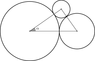
Figure 2. Here, all circles are tangent. If the central circle has radius $1$ and the other two have radii $r$ and $s$, then the law of cosines gives $(r+s)^{2}=(1+r)^{2}+(1+s)^{2}-2(1+r)(1+s)\cos\alpha$.

Say two interior-disjoint balls of radii $r$ and $s$ touch a central unit ball and let $x$ and $y$ be the contact points between each of the balls and the central ball. Apply the law of cosines (see Figure 2) to get

$$x\cdot y\leq\frac{1+r+s-rs}{1+r+s+rs}.$$ (1)

Denote the right-hand side above by $\operatorname{ip}(r,s)$.

If $F\colon[0,1]^{2}\to\mathbb{R}$ is a kernel and $U\subseteq[0,1]$ is a finite set, then the matrix $\bigl{(}F(u,v)\bigr{)}_{u,v\in U}$ is a principal submatrix of $F$. We denote by $P_{k}^{n}$ the Jacobi polynomial of degree $k$ and parameters $\alpha=\beta=(n-3)/2$, normalized so $P_{k}^{n}(1)=1$ (see the book by Szegö [17] for background on Jacobi polynomials).

The following theorem is our basic tool to find upper bounds for $\operatorname{dens}_{n}(\rho)$.

Theorem 3.1.

Let $n\geq 3$ be an integer, $\rho$ be such that $1<\rho<3$, and $R$ be such that $R>(\rho-1)/2$. Let $r$ be an increasing bijection from $[0,1]$ to $[(\rho-1)/2,R]$ and let $a\colon[0,1]\to\nobreak\mathbb{R}$ be such that $a(u)\geq A_{n,\rho}(r(u))^{1/2}$ for all $u\in[0,1]$ and $a(1)\geq\nobreak A_{n,\rho}(\infty)^{1/2}$.

Fix an integer $d>0$ and for every $k=0$, …, $d$ let $F_{k}\colon[0,1]^{2}\to\mathbb{R}$ be a kernel; write

$$f(t,u,v)=\sum_{k=0}^{d}F_{k}(u,v)P_{k}^{n}(t)\qquad\text{for~{}$t\in[-1,1]$ and~{}$u$, $v\in[0,1]$.}$$ (2)

If $f$ and the kernels $F_{k}$ are such that

1. every principal submatrix of $F_{0}-a\otimes a^{*}$ is positive semidefinite,

2. every principal submatrix of $F_{k}$ is positive semidefinite for $k=0$, …, $d$, and

3. $f(t,u,v)\leq 0$ whenever $-1\leq t\leq\operatorname{ip}(r(u),r(v))$,

then $\operatorname{dens}_{n}(\rho)\leq\max\{\,f(1,u,u):u\in[0,1]\,\}$.

This theorem is very similar to Theorem 1.2 of de Laat, Oliveira, and Vallentin [12]. They consider configurations of spherical caps of different radii, but the radii are taken from a finite list of possibilities; then the function $f$ is matrix valued. Here we work with configurations of balls of different radii, and the list of possible radii is infinite, namely the interval $[(\rho-1)/2,R]$. For this reason we work with the function $f$ as defined in the theorem above; $f$ can be seen as a kernel-valued function that assigns to each $t\in[-1,1]$ a kernel on $[0,1]^{2}$.

Proof.

Consider any configuration $\mathcal{P}$ of interior-disjoint balls of any radii tangent to the unit ball centered at the origin. Let $\Delta$ be the normalized area of $\rho S^{n-1}$ covered by this configuration and assume $\Delta>0$. Since a ball of radius less than $(\rho-1)/2$ tangent to the central unit ball does not intersect $\rho S^{n-1}$, we assume that each ball in $\mathcal{P}$ has radius at least $(\rho-1)/2$.

Given a ball $B\in\mathcal{P}$, consider the point $x\in S^{n-1}$ where it touches the central unit ball. If the radius of $B$ is in the interval $[(\rho-1)/2,R]$, then let $u\in[0,1]$ be such that $r(u)$ is the radius of $B$; otherwise, set $u=1$. Now $B$ will be represented by the pair $(x,u)$; let $I\subseteq S^{n-1}\times[0,1]$ be the set of pairs representing each ball in $\mathcal{P}$.

We will need the following claim: if every principal submatrix of $F\colon[0,1]^{2}\to\mathbb{R}$ is positive semidefinite and if $k\geq 0$ is an integer, then the matrix

$$\bigl{(}F(u,v)P_{k}^{n}(x\cdot y)\bigr{)}_{(x,u),(y,v)\in I}$$

is positive semidefinite.

The proof of this claim is as follows. Write

$$\begin{split}S&=\{\,x\in S^{n-1}:\text{$(x,u)\in I$ for some~{}$u\in[0,1]$}\,\}\quad\text{and}\\ T&=\{\,u\in[0,1]:\text{$(x,u)\in I$ for some~{}$x\in S^{n-1}$}\,\}.\end{split}$$

The addition theorem for Gegenbauer polynomials [2, Theorem 9.6.3] implies that there is a real finite-dimensional Hilbert space $H$ and vectors $p(x)\in H$ for $x\in S$ such that $P_{k}^{n}(x\cdot y)=\langle p(x),p(y)\rangle$ for all $x$, $y\in S$, where $\langle\cdot,\cdot\rangle$ denotes the inner product in $H$. Similarly, since every principal submatrix of $F$ is positive semidefinite, there is a real finite-dimensional Hilbert space, which we may assume to be $H$ as well, and vectors $q(u)\in H$ for $u\in T$ such that $F(u,v)=\langle q(u),q(v)\rangle$ for all $u$, $v\in T$. But then

$$F(u,v)P_{k}^{n}(x\cdot y)=\langle p(x)\otimes q(u),p(y)\otimes q(v)\rangle$$

for all $(x,u)$, $(y,v)\in I$, and the claim follows.

Since $P_{0}^{n}$ is the constant one polynomial, the claim just proved together with (i), (ii), and the definition of $f$ implies that the matrix

$$\bigl{(}f(x\cdot y,u,v)-a(u)a(v)\bigr{)}_{(x,u),(y,v)\in I}$$

is positive semidefinite. Hence

$$\sum_{(x,u),(y,v)\in I}f(x\cdot y,u,v)a(u)a(v)-a(u)^{2}a(v)^{2}\geq 0.$$

Since $\mathcal{P}$ is a configuration of interior-disjoint balls, if $(x,u)$, $(y,v)\in I$ then $-1\leq x\cdot y\leq\operatorname{ip}(r(u),r(v))$. Now use (iii) and split the sum on the left-hand side above into the diagonal and off-diagonal terms to get the inequality

$$\begin{split}0&\leq\sum_{(x,u),(y,v)\in I}f(x\cdot y,u,v)a(u)a(v)-a(u)^{2}a(v)^{2}\\ &\leq\sum_{(x,u)\in I}f(1,u,u)a(u)^{2}-\Biggl{(}\sum_{(x,u)\in I}a(u)^{2}\Biggr{)}^{2},\end{split}$$

so

$$\sum_{(x,u)\in I}a(u)^{2}\leq\max\{\,f(1,u,u):u\in[0,1]\,\}.$$

Finally, by the construction of $I$ and the properties satisfied by $a$ we know that $\Delta$ is at most the left-hand side above, and so the theorem follows. ∎

To use Theorem 3.1 we need to specify the kernels $F_{k}$. One way to do so is to fix an integer $N>0$ and functions $p_{0}$, …, $p_{N}\colon[0,1]\to\mathbb{R}$. Then, given a matrix $A\in\mathbb{R}^{(N+1)\times(N+1)}$, set

$$F(u,v)=\sum_{i,j=0}^{N}A_{ij}p_{i}(u)p_{j}(v).$$

It is easy to check that, if $A$ is positive semidefinite, then every principal submatrix of $F$ is positive semidefinite. Similarly, if $a=\alpha_{0}p_{0}+\cdots+\alpha_{N}p_{N}$ and the matrix $\bigl{(}A_{ij}-\alpha_{i}\alpha_{j}\bigr{)}_{i,j=0}^{N}$ is positive semidefinite, then every principal submatrix of $F-a\otimes a^{*}$ is positive semidefinite.

In this way, Theorem 3.1 can be rephrased as a semidefinite program. By choosing different functions $p_{0}$, …, $p_{N}$, one obtains different optimization problems, and there is an interplay between the functions chosen to specify the kernels and the quality of the approximation $a$ of $u\mapsto A_{n,\rho}(r(u))^{1/2}$ that one can obtain. In the next two sections we will use this approach to construct optimization problems that give bounds for $\operatorname{dens}_{n}(\rho)$ that lead to the new upper bounds for the average kissing number in Table 1; for the functions $p$ we will take alternately step functions and polynomials.

3.1. Step functions

Let us first set the $p_{i}$ to be step functions. Fix $R>(\rho-1)/2$ and let $r\colon[0,1]\to[(\rho-1)/2,R]$ be such that

$$r(u)=(R-(\rho-1)/2)u+(\rho-1)/2.$$ (3)

Note that $r$ is an increasing bijection between $[0,1]$ and $[(\rho-1)/2,R]$.

Now fix an integer $N>0$ and points $0=s_{0}<s_{1}<\cdots<s_{N}<s_{N+1}=1$. Let $S_{i}=[s_{i},s_{i+1})$ for $i=0$, …, $N-1$ and $S_{N}=[s_{N},s_{N+1}]$. Let $p_{i}$ be the function that is $1$ on $S_{i}$ and $0$ everywhere else.

The function $a$ is now simple to specify: for $u\in[0,1]$ set

$$a(u)=\begin{cases}A_{n,\rho}(r(s_{i+1}))^{1/2}&\text{if~{}$u\in S_{i}$ for some~{}$i<N$};\\ A_{n,\rho}(\infty)^{1/2}&\text{if~{}$u\in S_{N}$.}\end{cases}$$

Then $a$ is an upper approximation of the function $u\mapsto A_{n,\rho}(r(u))^{1/2}$ (since this is a monotonically increasing function) as needed in Theorem 3.1, and moreover $a$ is a linear combination of the $p_{i}$ functions.

Each kernel $F_{k}$ is parameterized by an $(N+1)\times(N+1)$ positive-semidefinite matrix $A_{k}$ as follows:

$$F_{k}(u,v)=\sum_{i,j=0}^{N}A_{k,ij}p_{i}(u)p_{j}(v)\qquad\text{for all~{}$u$, $v\in[0,1]$},$$

where $A_{k,ij}=(A_{k})_{ij}$. So the kernels $F_{k}$ are constant on the sets $S_{i}\times S_{j}$, and therefore $F_{k}$ can be quite naturally identified with $A_{k}$. For fixed $u$, $v\in[0,1]$, the function $t\mapsto f(t,u,v)$ defined in (2) is a polynomial on $t$; for $i$, $j=0$, …, $N$ we write $f_{ij}(t)$ for the common value that $f(t,u,v)$ assumes on $S_{i}\times S_{j}$, that is,

$$f_{ij}(t)=f(t,s_{i},s_{j})=\sum_{k=0}^{d}\sum_{i,j=0}^{N}A_{k,ij}p_{i}(s_{i})p_{j}(s_{j})P_{k}^{n}(t)=\sum_{k=0}^{d}A_{k,ij}P_{k}^{n}(t).$$

Say that $u\in S_{i}$ and $v\in S_{j}$; from (1) we have $\operatorname{ip}(r(u),r(v))\leq\operatorname{ip}(r(s_{i}),r(s_{j}))$. So to ensure that $f$ satisfies item (iii) of Theorem 3.1 we have to ensure that, for all $i$, $j=0$, …, $N$,

$$f_{ij}(t)\leq 0\qquad\text{whenever~{}$-1\leq t\leq\operatorname{ip}(r(s_{i}),r(s_{j}))$}.$$ (4)

Summarizing, if $a=\alpha_{0}p_{0}+\cdots+\alpha_{N}p_{N}$, then any feasible solution of the following optimization problem gives an upper bound for $\operatorname{dens}_{n}(\rho)$:

$${\begin{array}[]{r@{\ }l@{\quad}l}\min&\lx@intercol\max\{\,f_{ii}(1):\text{$i=0$, \ldots,~{}$N$}\,\}\hfil\lx@intercol\\ &\lx@intercol f_{ij}(t)=\sum_{k=0}^{d}A_{k,ij}P_{k}^{n}(t),\hfil\lx@intercol\\[4.30554pt] &f_{ij}(t)\leq 0&\text{whenever $-1\leq t\leq\operatorname{ip}(r(s_{i}),r(s_{j}))$},\\ &\bigl{(}A_{0,ij}-\alpha_{i}\alpha_{j}\bigr{)}_{i,j=0}^{N}&\text{is positive semidefinite,}\\[4.30554pt] &A_{k}\in\mathbb{R}^{(N+1)\times(N+1)}&\text{is positive semidefinite for~{}$k=0$, \ldots,~{}$d$.}\end{array}}$$ (5)

To model the nonpositivity constraints on the functions $f_{ij}$ we ensure nonpositivity on a finite sample of points in $[-1,\operatorname{ip}(r(s_{i}),r(s_{j}))]$. For the complete approach and a description of how the solutions found by a solver can be rigorously verified, see Appendix B.

Problem 5 can be used to give better bounds for the average kissing number in dimensions $5$, …, $9$; see Table 1. In dimension $3$, we could not beat Glazyrin’s bound using this problem; in dimension $4$, the bound provided is better than Glazyrin’s bound, but worse than the bound of §3.2 below. To obtain the bounds of Table 1, we used $\rho=2$, $N=30$, and $R\approx 184.25$; see the verification script (cf. Appendix B) for precise information.

3.2. Polynomials

We now take the functions $p_{i}$ to be polynomials. Fix an integer $N>0$ and let $p_{i}(u)=u^{i}$ for $i=0$, …, $N$. Fix $R>(\rho-1)/2$ and let $r\colon[0,1]\to[(\rho-1)/2,R]$ be such that

$$r(u)=(R-(\rho-1)/2)u^{2}+(\rho-1)/2.$$ (6)

Note that $r$ is an increasing bijection between $[0,1]$ and $[(\rho-1)/2,R]$. Note also that, in comparison with (3), we have $u^{2}$ instead of $u$ above; we could use $u$, but we noticed that this leads to a worse upper approximation $a$.

To get the function $a$ we solve a simple linear program that is set up as follows. We have variables $\alpha_{0}$, …, $\alpha_{N}$ for the coefficients of $p_{0}$, …, $p_{N}$. We fix some $\epsilon\geq 0$ and a finite sample $S$ of points in $[0,1]$ and consider the constraints

$$\begin{array}[]{ll}\alpha_{0}p_{0}(u)+\cdots+\alpha_{N}p_{N}(u)\geq A_{n,\rho}(r(u))^{1/2}+\epsilon&\text{for~{}$u\in S$},\\ \alpha_{0}p_{0}(1)+\cdots+\alpha_{N}p_{N}(1)\geq A_{n,\rho}(\infty)^{1/2}.\end{array}$$

The objective is to minimize

$$\max\{\,\alpha_{0}p_{0}(u)+\cdots+\alpha_{N}p_{N}(u)-A_{n,\rho}(r(u))^{1/2}:u\in S\,\}.$$

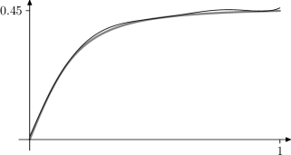
Figure 3. A polynomial of degree 6 (in black) that approximates $u\mapsto A_{3,\sqrt{3}}(r(u))^{1/2}$ (in gray) from above; here we take $R=\nobreak 30$. Note the jump at the end to make $a(1)\geq A_{3,\sqrt{3}}(\infty)$.

By taking a fine enough sample of points and a small positive $\epsilon\approx 10^{-5}$, the function $a=\alpha_{0}p_{0}+\cdots+\alpha_{N}p_{N}$ will satisfy the properties in Theorem 3.1, though this has to be verified (see Appendix C.1). If $N$ is large enough, the function $a$ should also be close enough to $u\mapsto A_{n,\rho}(r(u))^{1/2}$ (see Figure 3).

Each kernel $F_{k}$ is parameterized by an $(N+1)\times(N+1)$ positive-semidefinite matrix $A_{k}$ as follows:

$$F_{k}(u,v)=\sum_{i,j=0}^{N}A_{k,ij}p_{i}(u)p_{j}(v)\qquad\text{for all~{}$u$, $v\in[0,1]$}.$$

So the function $f$ defined in (2) is a polynomial on $t$, $u$, and $v$. Recalling (1), item (iii) in Theorem 3.1 then asks that $f(t,u,v)$ should be nonpositive on the semialgebraic set $\{\,(t,u,v):\text{$s_{i}(t,u,v)\geq 0$ for~{}$i=1$, \ldots,~{}$4$}\,\}$, where the $s_{i}$ are the following polynomials:

$$\begin{split}s_{1}&=t+1,\\ s_{2}&=1+r(u)+r(v)-r(u)r(v)-t(1+r(u)+r(v)+r(u)r(v)),\\ s_{3}&=u(1-u)+v(1-v),\quad\text{and}\\ s_{4}&=u(1-u)v(1-v);\end{split}$$ (7)

note that $s_{3}(t,u,v)\geq 0$ and $s_{4}(t,u,v)\geq 0$ if and only if $0\leq u\leq 1$ and $0\leq v\leq 1$.

The nonpositivity condition can then be restricted to a sum-of-squares condition: we require that there exist polynomials $q_{1}$, …, $q_{5}$, each a sum of squares, such that

$$f=-s_{1}q_{1}-s_{2}q_{2}-s_{3}q_{3}-s_{4}q_{4}-q_{5},$$ (8)

since then $f$ is clearly nonpositive in the required domain.

Finally, the upper bound on $\operatorname{dens}_{n}(\rho)$ is given by the maximum value of the function $u\mapsto f(1,u,u)$ on $[0,1]$; note that this function is a univariate polynomial on $u$ of degree $2N$. A theorem of Lukács [17, Theorem 1.21.1] says that this maximum is equal to the minimum $\lambda$ for which there are univariate polynomials $l_{1}$ and $l_{2}$, each a sum of squares, such that

$$\lambda-f(1,u,u)=l_{1}(u)+u(1-u)l_{2}(u).$$ (9)

Putting it all together, we get the following optimization problem, any feasible solution of which gives an upper bound for $\operatorname{dens}_{n}(\rho)$:

$${\begin{array}[]{r@{\ }l@{\quad}l}\min&\lambda\\ &f(t,u,v)=\sum_{k=0}^{d}\sum_{i,j=0}^{N}A_{k,ij}p_{i}(u)p_{j}(v)P_{k}^{n}(t),\\[4.30554pt] &\text{$q_{1}$, \ldots,~{}$q_{5}$ are sum-of-squares polynomials satisfying~{}\eqref{eq:sos-f},}\\[4.30554pt] &\text{$l_{1}$ and $l_{2}$ are sum-of-squares polynomials satisfying~{}\eqref{eq:sos-obj},}\\[4.30554pt] &\text{$\bigl{(}A_{0,ij}-\alpha_{i}\alpha_{j}\bigr{)}_{i,j=0}^{N}$ is positive semidefinite,}\\[4.30554pt] &\text{$A_{k}\in\mathbb{R}^{(N+1)\times(N+1)}$ is positive semidefinite for~{}$k=0$, \ldots,~{}$d$.}\end{array}}$$ (10)

Problem (10) can be rewritten as a semidefinite program, where each sum-of-squares polynomial is parameterized by a positive-semidefinite matrix. Appendix C.2 gives a detailed description of the semidefinite program we solve and an overview of how the solution found by the solver can be verified to be feasible.

The approach of this section provides better bounds for the average kissing number in dimensions $3$ and $4$; see Table 1. In higher dimensions we could not manage to obtain any bounds using this approach, since the problems are infeasible when polynomials of low degree are used, and too large when polynomials of high degree are used.

4. A direct linear programming bound

Suppose we want to find the average kissing number, but that we restrict ourselves to packings having balls of a few prescribed radii, say $r_{1}<\cdots<r_{N}$. How many neighbors can a vertex in the contact graph of such a packing have? Or, in other words, how many balls can touch a given ball in the packing? Certainly, the largest number of balls touching a central ball is attained when the central ball has the largest possible radius, $r_{N}$, and every ball touching it has the smallest possible radius, $r_{1}$. Hence the maximum degree of the contact graph, and by consequence its average degree, is at most the maximum number of interior-disjoint balls of radius $r_{1}$ that can simultaneously touch a central ball of radius $r_{N}$.

This is a simple upper bound for this restricted average kissing number, but one could object it is too local: the bound does not take the whole packing into account, ignoring the interaction between different balls. In particular, it is usually impossible for every vertex in the packing to have the maximum possible degree, since not every vertex can be the largest ball surrounded by several small balls.

The bound for the average kissing number given by Theorem 2.2 appears to be similarly local. It is based on the parameter $\operatorname{dens}_{n}(\rho)$, which is not defined in terms of a packing of balls and therefore cannot take into account the interaction between different balls in a packing. We discuss now an alternative idea, based on the linear programming bound of Cohn and Elkies [3] for the sphere packing density, which seems to overcome this issue.

A continuous (matrix-valued) function $f\colon\mathbb{R}^{n}\to\mathbb{R}^{N\times N}$ is of positive type if for every finite set $U\subseteq\mathbb{R}^{n}$ the block matrix

$$\bigl{(}f(x-y)\bigr{)}_{x,y\in U}$$

is positive semidefinite. Matrix-valued functions of positive type are straightforward extensions of functions of positive type; see e.g. the paper by de Laat, Oliveira, and Vallentin [12, §3] for more on such functions.

Theorem 4.1.

Let $r_{1}$, …, $r_{N}$ be any positive numbers. If $f\colon\mathbb{R}^{n}\to\mathbb{R}^{N\times N}$ is a continuous function of positive type such that

1. $f(x)_{ij}\leq 0$ if $\|x\|\geq r_{i}+r_{j}$ and

2. $f(x)_{ij}\leq-1$ if $\|x\|=r_{i}+r_{j}$,

then the average degree of the contact graph of a packing of balls of radii $r_{1}$, …, $r_{N}$ is at most $\max\{\,f(0)_{ii}:\text{$i=1$, \ldots,~{}$N$}\,\}$.

Proof.

Let $\mathcal{P}$ be a packing of balls of radii $r_{1}$, …, $r_{N}$ and let $I\subseteq\{1,\ldots,N\}\times\mathbb{R}^{n}$ be such that $(i,x)\in I$ if and only if $\mathcal{P}$ has a ball of radius $r_{i}$ centered at $x$. Since $f$ is of positive type we know that

$$\sum_{(i,x),(j,y)\in I}f(x-y)_{ij}\geq 0.$$

Let $G=(\mathcal{P},E)$ be the contact graph of the packing $\mathcal{P}$. Split the sum above into three parts: the diagonal terms, the terms corresponding to pairs of balls that do not touch, and the terms corresponding to pairs of balls that do touch. Since $f$ satisfies (i) and (ii) we get

$$\begin{split}0&\leq\sum_{(i,x)\in I}f(0)_{ii}+\sum_{\begin{subarray}{c}(i,x),(j,y)\in I\\ r_{i}+r_{j}\neq\|x-y\|\end{subarray}}f(x-y)_{ij}+\sum_{\begin{subarray}{c}(i,x),(j,y)\in I\\ r_{i}+r_{j}=\|x-y\|\end{subarray}}f(x-y)_{ij}\\ &\leq\sum_{(i,x)\in I}f(0)_{ii}-2|E|\\ &\leq|I|\max\{\,f(0)_{ii}:\text{$i=1$, \ldots,~{}$N$}\,\}-2|E|,\end{split}$$

whence $2|E|/|\mathcal{P}|\leq\max\{\,f(0)_{ii}:\text{$i=1$, \ldots,~{}$N$}\,\}$, and the theorem follows. ∎

This theorem gives a direct bound for the average kissing number instead of the rather indirect bound of Theorem 2.2 via the parameter $\operatorname{dens}_{n}(\rho)$. Moreover, we have a two-point bound, that takes into account interactions between pairs of balls in a packing.

Though Theorem 4.1 is stated for a finite number of possible radii, it can be easily extended to account for radii in any bounded interval $[a,b]$ if one uses kernel-valued functions. It is not immediately clear, however, how to adapt the theorem for packings of balls of arbitrary radii, and so Theorem 4.1 cannot be directly used to compute upper bounds for the average kissing number.

For any given radii $r_{1}$, …, $r_{N}$, it is possible to reduce the problem of finding functions satisfying the conditions in Theorem 4.1 to a semidefinite program; such a reduction was employed by de Laat, Oliveira, and Vallentin [12, §5] for a similar problem. In this way, concrete bounds can be computed.

The bound of Theorem 2.2 can be adapted to packings of balls of finitely many possible radii $r_{1}$, …, $r_{N}$, namely by changing the definition of $\operatorname{dens}_{n}(\rho)$. Fix $k=1$, …, $N$ and $\rho>1$; consider the unit ball centered at the origin. Any configuration of pairwise interior-disjoint balls of radii $r_{i}/r_{k}$, for $i=1$, …, $N$, covers a certain fraction of the sphere $\rho S^{n-1}$ of radius $\rho$ centered at the origin. Denote the supremum of this covered fraction, taken over all such configurations, by $\operatorname{dens}_{n}^{k}(\rho)$, and let

$$\operatorname{dens}_{n}(\rho)=\max\{\operatorname{dens}_{n}^{1}(\rho),\ldots,\operatorname{dens}_{n}^{N}(\rho)\}.$$

Following the proof of Theorem 2.2, we see that the average degree of the contact graph of any packing of balls of radii $r_{1}$, …, $r_{N}$ is at most

$$\frac{\operatorname{dens}_{n}(\rho)}{A_{n,\rho}(1)}.$$

Upper bounds for $\operatorname{dens}_{n}^{k}(\rho)$ can be computed using the approach of de Laat, Oliveira, and Vallentin [12, Theorem 1.2].

So it is possible to compare numerically, for different choices of radii, bounds given by Theorem 4.1 with bounds given by Theorem 2.2. The case $N=1$ is particularly simple, since then $\operatorname{dens}_{n}(\rho)$ is the kissing number $\tau_{n}$ of $\mathbb{R}^{n}$ times the area covered by the spherical cap, which is $A_{n,\rho}(1)$. So

$$\frac{\operatorname{dens}_{n}(\rho)}{A_{n,\rho}(1)}=\tau_{n},$$

and moreover any upper bound for the kissing number, like the linear programming bound of Delsarte, Goethals, and Seidel [5], gives an upper bound for the average degree of the contact graph. As for Theorem 4.1, we have observed numerically that it provides a worse upper bound than the linear programming bound for the kissing number. Surprisingly, when more than one radius is considered, the bound of Theorem 4.1 becomes even worse; Table 2 contains some results.

Radii	Adapted Theorem 2.2	Theorem 4.1
$1$	13.159	13.402
$1/2$, $1$	13.219	14.877
$1/3$, $1$	13.159	17.294
$1/4$, $1$	13.159	19.981
$1/5$, $1$	13.159	22.770
$1/6$, $1$	13.159	25.651
$1/3$, $1/2$, $1$	13.311	17.294
$1/4$, $1/2$, $1$	13.283	19.981
$1/4$, $1/3$, $1$	13.310	19.981
$1/5$, $1/3$, $1$	13.281	22.770
$1/4$, $1/3$, $1/2$, $1$	13.320	19.981

Table 2. Comparison between bounds for the average degree of contact graphs of packings of balls of given radii in dimension 3 given by the adaptation of Theorem 2.2 and Theorem 4.1. These bounds have been computed numerically.

Appendix A Computing the area of a spherical cap

To use Theorem 3.1 we need to be able to compute the normalized area of a spherical cap of radius $\alpha$ in $S^{n-1}$, which is given by

$$\frac{\omega(S^{n-2})}{\omega(S^{n-1})}\int_{\cos\alpha}^{1}(1-u^{2})^{(n-3)/2}\,du.$$

The factor before the integral can be computed, to any desired precision, by means of a recurrence. We will now derive a recurrence relation for the integral above, making it possible to compute the normalized area to any desired precision.

Let $s$ be a real number. The Taylor series of $u\mapsto(1-u)^{s}$ around $0$ is

$$\sum_{k=0}^{\infty}(-1)^{k}s(s-1)\cdots(s-k+1)\frac{u^{k}}{k!}=\sum_{k=0}^{\infty}(-s)_{k}\frac{u^{k}}{k!},$$

where for a real number $a$ and an integer $k\geq 0$ we denote by $(a)_{k}$ the shifted factorial:

$$(a)_{k}=\begin{cases}1,&\text{if~{}$k=0$;}\\ a(a+1)\cdots(a+k-1),&\text{otherwise.}\end{cases}$$

Substitute $u$ by $u^{2}$ and integrate term-by-term to get

$$\int(1-u^{2})^{s}\,du=\sum_{k=0}^{\infty}(-s)_{k}\frac{u^{2k+1}}{(2k+1)k!}=u\,{}_{2}F_{1}(1/2,-s;3/2;u^{2}),$$

where ${}_{2}F_{1}$ is the hypergeometric series [1, Chapter 15].

So we want to compute

$$F_{n}(u)={}_{2}F_{1}(1/2,-(n-3)/2;3/2;u^{2}).$$

Equation (15.2.11) in the book by Abramovitz and Stegun [1] gives us the relation

$$(c-b)\,{}_{2}F_{1}(a,b-1;c;z)+(2b-c-bz+az)\,{}_{2}F_{1}(a,b;c;z)\\ +b(z-1)\,{}_{2}F_{1}(a,b+1;c;z)=0.$$

Take $a=1/2$, $b=-(n-3)/2$, and $c=3/2$ to get an expression for $F_{n+2}(u)$ in terms of $F_{n}(u)$ and $F_{n-2}(u)$. It is now easy to obtain a recurrence; the base cases are

$$F_{3}(u) =1, F_{4}(u) =\frac{u(1-u^{2})^{1/2}+\arcsin u}{2u},$$

$$F_{5}(u) =1-u^{2}/3,\qquad\text{and} F_{6}(u) =\frac{u(5-2u^{2})(1-u^{2})^{1/2}+3\arcsin u}{8u}.$$

Appendix B The semidefinite program for step functions and rigorous verification

For each $i$, $j=0$, …, $N$, to implement the nonpositivity constraint for $f_{ij}$ in problem (5) we select a finite sample $\mathcal{S}_{ij}$ of points in $[-1,\operatorname{ip}(r(s_{i}),r(s_{j}))]$. Consider the matrix $W$ such that $W_{ij}=\alpha_{i}\alpha_{j}$ and fix $\epsilon>0$. To obtain an upper bound we solve the following semidefinite program, in which the role of the $A_{0}$ variable changes in comparison with (5):

$${\begin{array}[]{r@{\ }l@{\quad}l}\min&\max\{\,f_{ii}(1):\text{$i=0$, \ldots,~{}$N$}\,\}\\ &f_{ij}(t)=W_{ij}+\sum_{k=0}^{d}A_{k,ij}P_{k}^{n}(t),\\ &\text{$f_{ij}(t)\leq-\epsilon$\quad for~{}$t\in\mathcal{S}_{ij}$},\\ &\text{$A_{k}\in\mathbb{R}^{(N+1)\times(N+1)}$ is positive semidefinite for~{}$k=0$, \ldots,~{}$d$.}\end{array}}$$ (11)

In practice, we select samples of 50 points for each $i$, $j$ and set $\epsilon=10^{-5}$. We solve the resulting problem with standard solvers and obtain a tentative optimal value $z^{*}$. The next step is to remove the objective function and add it as a constraint, requiring that

$$\max\{\,f_{ii}(1):\text{$i=0$, \ldots,~{}$N$}\,\}\leq z^{*}+\eta,$$

where $\eta\approx 10^{-3}$. When we solve this feasibility problem, the solver returns a strictly feasible solution, that is, a solution in which every matrix $A_{k}$ is positive definite. We observed that this solution immediately satisfies the original nonpositivity constraints of (5).

To verify that we have indeed a feasible solution, we only have to verify that each $A_{k}$ is positive semidefinite and compute an upper bound on the value of $f_{ij}$ on $[-1,\operatorname{ip}(r(s_{i}),r(s_{j}))]$. Since each $A_{k}$ is actually positive definite, we use high-precision floating-point arithmetic to compute for each $A_{k}$ its Cholesky decomposition $L_{k}$. Then we replace $A_{k}$ by $L_{k}L_{k}^{\sf T}$, so $A_{k}$ becomes positive semidefinite by construction.

To get an upper bound for the value of $f_{ij}$ on the corresponding interval, we use interval arithmetic. We split the original interval into subintervals and evaluate $f_{ij}$ on each subinterval, obtaining for each subinterval an upper bound on the value of $f_{ij}$. In this way, we obtain an upper bound $u_{ij}$ on the value of $f_{ij}$ on the original interval.

Since the definition of $f_{ij}$ uses $W$, which in practice is computed numerically, it is not enough to have $u_{ij}\leq 0$. Indeed, if we use the exact value of $W_{ij}$ instead of an approximation, then $f_{ij}$ could change to a positive number. To prevent this from happening, we need to ensure that $u_{ij}$ is negative enough compared to the absolute error in the computation of $W_{ij}$. If we use the formulas of Appendix A to compute $W_{ij}$ using high-precision interval arithmetic, then we have a rigorous bound on the absolute error of each $W_{ij}$. This whole verification approach is implemented in a Sage [15] script included with the arXiv version of this paper.

Appendix C The semidefinite program for polynomial interpolation and rigorous verification

Two steps are required in order to obtain rigorous upper bounds for the average kissing number via the approach of §3.2. First, we must find a polynomial that approximates the spherical-cap-area function from above, and we must prove that this polynomial is really an upper bound for this function. Second, we must rewrite problem (10) as a semidefinite program, find good solutions for it, and prove that they are feasible. In this section, we will see how both steps can be carried out.

C.1. Verifying the approximation for $A_{n,\rho}$

In §3.2 we have seen how a polynomial $a$ satisfying the conditions described in Theorem 3.1 can be found. Here we quickly describe how it can be rigorously verified that a given polynomial $a$ satisfies these conditions; this verification approach is implemented in a Sage [15] script included with the arXiv version of this paper.

Say $\rho$ and $R$ are fixed and let $r(u)$ be defined as in (6). We want to prove that $a(u)^{2}-A_{n,\rho}(r(u))\geq 0$ for all $u\in[0,1]$ and moreover that $a(1)^{2}-A_{n,\rho}(\infty)\geq 0$; the difficulty lies in testing the validity of the first set of conditions.

Say we have an upper bound $M$ on the absolute value of the derivative of the function $f(u)=a(u)^{2}-A_{n,\rho}(r(u))$ on the interval $[0,1]$. For an integer $N\geq 1$, write $\epsilon=1/(N+1)$ and consider the points $u_{k}=k\epsilon$ for $k=0$, …, $N+1$. If $\eta$ is the minimum of $f$ on the points $u_{k}$, then the mean-value theorem implies that

$$f(u)\geq\eta-\epsilon M/2\qquad\text{for all~{}$u\in[0,1]$.}$$

So, as long as $\eta-\epsilon M/2\geq 0$, the function $f$ is nonnegative on $[0,1]$. Computing the function $f$ on lots of points yields a guess for $\eta$; then we find $N$ such that $\epsilon=1/(N+1)\leq 2\eta/M$ and try to test the function on the points $u_{k}$. This is the approach implemented in the verification script.

It remains to see how to compute the upper bound $M$ on the absolute value of the derivative of $f$. Since $a(u)$, and hence $a(u)^{2}$, is a polynomial, it is easy to compute an upper bound on the absolute value of the derivative of $a(u)^{2}$ rigorously using interval arithmetic.

Bounding the derivative of $A_{n,\rho}(r(u))$ is also simple. Indeed, recall that $A_{n,\rho}(s)$ equals

$$\frac{\omega(S^{n-2})}{\omega(S^{n-1})}\int_{x}^{1}(1-z^{2})^{(n-3)/2}\,dz,$$

where

$$x=\frac{\rho^{2}+2s+1}{2\rho(1+s)}.$$

So

$$A_{n,\rho}^{\prime}(s)=-\frac{\omega(S^{n-2})}{\omega(S^{n-1})}(1-x^{2})^{(n-3)/2}\frac{\rho^{2}-1}{2\rho(1+s)^{2}}.$$

Note that $0\leq x\leq 1$, so $|(1-x^{2})^{(n-3)/2}|\leq 1$. The rightmost fraction above is largest when $s=0$ and $|r^{\prime}(u)|=|2(R-(\rho-1)/2)u|\leq 2(R-(\rho-1)/2)$ for $u\in[0,1]$. Finally, apply the chain rule to get

$$\biggl{|}\frac{dA_{n,\rho}(r(u))}{du}\biggr{|}\leq\frac{\omega(S^{n-2})}{\omega(S^{n-1})}\frac{|\rho^{2}-1|}{\rho}(R-(\rho-1)/2)$$

for all $u\in[0,1]$.

C.2. The semidefinite program and how to verify feasibility

We quickly discuss how problem (10) is transformed into a semidefinite program and then how a provably feasible solution can be found for it.

To transform (10) into a semidefinite program, one has to encode each sum-of-squares polynomial in terms of positive-semidefinite matrices; here is the well-known recipe. Let $P_{1}$, …, $P_{m}$ be a basis of the space $\mathbb{R}[x_{1},\ldots,x_{n}]_{\leq k}$ of $n$-variable real polynomials of degree at most $k$ and for $x=(x_{1},\ldots,x_{n})$ let $v_{k}(x)$ be the vector such that

$$(v_{k}(x))_{i}=P_{i}(x)\qquad\text{for~{}$i=1$, \ldots,~{}$m$.}$$

We can see $v_{k}$ as a “vector” whose entries are the polynomials $P_{i}$.

A polynomial $p$ of degree $2k$ is a sum of squares if and only if there is a positive-semidefinite matrix $X$ such that

$$p(x)=\langle v_{k}(x)v_{k}(x)^{\sf T},X\rangle,$$

where $\langle A,B\rangle=\operatorname{tr}AB$ is the trace inner product between symmetric matrices $A$ and $B$. Note that above we have a polynomial identity: both the left and right-hand sides are polynomials that we require to be equal. This polynomial identity can be rewritten as a set of linear constraints on the entries of the matrix $X$: for each monomial of degree at most $2k$ we have one constraint relating the coefficient of the monomial on both left and right-hand sides.

The polynomials in (9) are univariate and have degree $2N$. So to model this constraint we use $v_{N}(u)=(1,u,u^{2},\ldots,u^{N})$.

Since the polynomial $f(t,u,v)$ is symmetric on $u$ and $v$, that is, $f(t,u,v)=f(t,v,u)$, and since the same holds for the polynomials $s_{1}$, …, $s_{4}$ in (7), we are able to further reduce the sizes of the positive-semidefinite matrices needed to encode (8).

Indeed, say that a sum-of-squares polynomial $p\in\mathbb{R}[t,u,v]$ is symmetric on $u$ and $v$. It is not necessarily true that there is a sum-of-squares decomposition $p=q_{1}^{2}+\cdots+q_{m}^{2}$ of $p$ in which every $q_{i}$ is symmetric. However, we have that

$$\mathbb{R}[t,u,v]=\mathbb{R}[t,u+v,uv]\oplus(u-v)\mathbb{R}[t,u+v,uv],$$

where $\mathbb{R}[t,u+v,uv]$ is the ring of polynomials symmetric on $u$ and $v$. So say $q_{i}=a_{i}+(u-v)b_{i}$, where $a_{i}$ and $b_{i}$ are symmetric. Then

$$\begin{split}p(t,u,v)&=(1/2)(p(t,u,v)+p(t,v,u))\\ &=\frac{1}{2}\sum_{i=1}^{m}a_{i}(t,u,v)^{2}+2(u-v)a_{i}(t,u,v)b_{i}(t,u,v)+(u-v)^{2}b_{i}(t,u,v)^{2}\\ &\phantom{=\frac{1}{2}\sum_{i=1}^{m}}\quad+a_{i}(t,v,u)^{2}+2(v-u)a_{i}(t,v,u)b_{i}(t,v,u)+(v-u)^{2}b_{i}(t,v,u)^{2}\\ &=\sum_{i=1}^{m}a_{i}(t,u,v)^{2}+(u-v)^{2}b_{i}(t,u,v)^{2}.\end{split}$$

For any given $k$, let $v_{k}(t,u,v)$ be obtained from a basis of $\mathbb{R}[t,u+v,uv]_{\leq k}$ as before. The above discussion implies that $p\in\mathbb{R}[t,u,v]$ of degree $2k$ is a symmetric sum of squares if and only if there are positive-semidefinite matrices $X$ and $X^{\prime}$ such that

$$p=\langle v_{k}v_{k}^{\sf T},X\rangle+\langle(u-v)^{2}v_{k-1}v_{k-1}^{\sf T},X^{\prime}\rangle.$$

Now it should be clear how (10) can be rewritten as a semidefinite program. Only one technical detail remains, namely how to determine the degrees of the sum-of-squares polynomials in (10). Here we use for each polynomial the smallest possible degree such that no term in the right-hand side of (8) has degree larger than $d+2N$, which is the degree of $f$.

The bounds for $n=3$ and $4$ in Table 1 were obtained by solving the semidefinite program described above with $d=10$ and $N=6$, $8$, respectively. To solve the problem we use the high-precision solver SDPA-GMP [14], but even so the solution found by the solver is not truly feasible. To extract a rational feasible solution from it we use the Julia library developed by Dostert, de Laat, and Moustrou [6]. This allows us to provide a rigorous upper bound for the average kissing number. The script to generate the semidefinite program and to obtain an exact rational solution is included with the arXiv version of this paper.

References

- [1] M. Abramowitz and I.A. Stegun, Handbook of mathematical functions with formulas, graphs, and mathematical tables, National Bureau of Standards Applied Mathematics Series 55, U.S. Government Printing Office, Washington, D.C., 1964.
- [2] G.E. Andrews, R. Askey, and R. Roy, Special Functions, Encyclopedia of Mathematics and its Applications 71, Cambridge University Press, Cambridge, 1999.
- [3] H. Cohn and N. Elkies, New upper bounds on sphere packings I, Annals of Mathematics 157 (2003) 689–714.
- [4] J.H. Conway and N.J.A. Sloane, Sphere Packings, Lattices, and Groups, Grundlehren der mathematischen Wissenschaften 290, Springer-Verlag, New York, 1988.
- [5] P. Delsarte, J.M. Goethals, and J.J. Seidel, Spherical codes and designs, Geometriae Dedicata 6 (1977) 363–388.
- [6] M. Dostert, D. de Laat, and P. Moustrou, Exact semidefinite programming bounds for packing problems, arXiv:2001.00256, 2020, 24pp.
- [7] D. Eppstein, G. Kuperberg, and G.M. Ziegler, Fat 4-polytopes and fatter 3-spheres, in: Discrete geometry, Monographs and Textbooks in Pure and Applied Mathematics 253, Dekker, New York, 2003, pp. 239–265.
- [8] A. Florian, Packing of incongruent circles on the sphere, Monatshefte für Mathematik 133 (2001) 111–129.
- [9] A. Florian, Remarks on my paper: “Packing of incongruent circles on the sphere”, Monatshefte für Mathematik 152 (2007) 39–43.
- [10] A. Glazyrin, Contact graphs of ball packings, arXiv:1707.02526, 2017, 15pp.
- [11] G. Kuperberg and O. Schramm, Average kissing numbers for non-congruent sphere packings, Mathematical Research Letters 1 (1994) 339–344.
- [12] D. de Laat, F.M. de Oliveira Filho, and F. Vallentin, Upper bounds for packings of spheres of several radii, Forum of Mathematics, Sigma 2 (2014) e23.
- [13] F.C. Machado and F.M. de Oliveira Filho, Improving the semidefinite programming bound for the kissing number by exploiting polynomial symmetry, Experimental Mathematics 27 (2018) 362–369.
- [14] M. Nakata, A numerical evaluation of highly accurate multiple-precision arithmetic version of semidefinite programming solver: SDPA-GMP,-QD and-DD, in: 2010 IEEE International Symposium on Computer-Aided Control System Design, 2010, pp. 29–34.
- [15] W.A. Stein et al., Sage Mathematics Software (Version 6.3), The Sage Development Team, 2014, http://www.sagemath.org.
- [16] K. Stephenson, Introduction to Circle Packing: The Theory of Discrete Analytic Functions, Cambridge University Press, Cambridge, 2005.
- [17] G. Szegö, Orthogonal Polynomials (Fourth Edition), American Mathematical Society Colloquium Publications Volume XXIII, American Mathematical Society, Providence, 1975.