Do Deep Minds Think Alike? Selective Adversarial Attacks for Fine-Grained Manipulation of Multiple Deep Neural Networks

Abstract

Recent works have demonstrated the existence of adversarial examples targeting a single machine learning system. In this paper we ask a simple but fundamental question of “selective fooling”: given multiple machine learning systems assigned to solve the same classification problem and taking the same input signal, is it possible to construct a perturbation to the input signal that manipulates the outputs of these multiple machine learning systems simultaneously in arbitrary pre-defined ways? For example, is it possible to selectively fool a set of “enemy” machine learning systems but does not fool the other “friend” machine learning systems? The answer to this question depends on the extent to which these different machine learning systems “think alike”. We formulate the problem of “selective fooling” as a novel optimization problem, and report on a series of experiments on the MNIST dataset. Our preliminary findings from these experiments show that it is in fact very easy to selectively manipulate multiple MNIST classifiers simultaneously, even when the classifiers are identical in their architectures, training algorithms and training datasets except for random initialization during training. This suggests that two nominally equivalent machine learning systems do not in fact “think alike” at all, and opens the possibility for many novel applications and deeper understandings of the working principles of deep neural networks.

1 Introduction

Recent works (Bhambri et al., 2019; Brunner et al., 2018; Carlini & Wagner, 2017; Kurakin et al., 2016; Goodfellow et al., 2014; Szegedy et al., 2013) have shown that the outputs of many machine learning systems can be significantly changed using very small carefully-chosen perturbations to the inputs. In many cases, it is possible to gain essentially complete control over the outputs of such systems with input perturbations that are imperceptible to human senses.

Such vulnerability to adversarial attacks poses a major challenge to building robust and reliable machine learning systems, and, as a result, understanding and mitigating this phenomenon has become a major focus of research. While this research has produced many interesting findings (Tramer et al., 2017; Carlini & Wagner, 2017; Fawzi et al., 2018; Brunner et al., 2018; Yi et al., 2019; Bhambri et al., 2019), theoretical explanations for, and practical defenses against, adversarial attacks both remain open problems at this time.

If we imagine machine learning systems to have perceptions, adversarial attacks can be thought of as illusions. This gives rise to the question: to what extent do different machine learning systems “see” the same features? In particular, we may ask whether two machine learning systems share the same illusions. We seek to answer this question by studying the extent to which it is possible to selectively manipulate multiple machine learning systems in different ways. In other words, we would like to know if it is possible to design input perturbations that simultaneously manipulate multiple machine learning systems into “seeing” different things.

The study of such more powerful attacks may help us understand the nature of adversarial attacks better. In addition, a study of such precise adversarial attacks may be of interest in its own right. For instance, the ability to precisely change the outputs of a set of selected machine learning systems while leaving other systems unaffected may allow the creation of adversarial attacks that fool “enemy” machine learning systems, but spare “friend” machine learning systems. This can potentially be useful in various security applications, for example, in evading detections by enemy forces in battlefields.

To our knowledge, adversarial attacks that selectively and differentially target multiple machine learning systems have not been studied in detail in previous works. However, many of the underlying ideas have been used in other contexts. Certainly, the idea of using multiple machine learning systems to augment each other in various ways in adversarial settings is not new. Many proposed defenses against adversarial attacks use auxiliary neural networks in various ways (Yin et al., 2019; Yi et al., 2019; Song et al., 2018; Samangouei et al., 2018), e.g., binary classifiers that are trained to detect adversarial inputs, or generative networks for retraining networks to reduce their vulnerability to such inputs. A common way to train adversarial generative networks is by using a discriminator network adversarially.

There also exists a significant volume of literature on transferability of adversarial attacks (Zheng et al., 2019; Lin et al., 2019; Kang et al., 2019; Adam et al., 2019; Fawzi et al., 2018; Tramer et al., 2017; Liu et al., 2016), i.e., the question of whether an attack designed for one machine learning system is effective against another system. Our formulation in this paper is related to transferability but is very different and significantly more general. Specifically, we consider adversarial perturbations that are simultaneously designed to attack multiple machine learning systems, and also to have potentially different effects on each attacked system. Before our investigation, even the existence of such highly precise and selective attacks is not clear. Our main objective in this paper is to investigate this selective attack, and perform an experimental study to provide preliminary answers to this and other related questions.

1.1 Summary of Objectives and Findings

Our overall objective is to construct adversarial attacks which selectively and precisely manipulate multiple machine learning systems. In particular, we seek general answers to the following fundamental questions.

1. How selective and precise can adversarial attacks be? Specifically, what is the largest number of different machine learning systems that can be simultaneously and selectively manipulated by the same adversarial input?

2. A trivial mathematical observation is that selective adversarial attacks targeting multiple machine learning systems simultaneously must require strictly larger perturbations than attacks targeting just one system. However, it is not clear how strong this relationship is. Thus, we would like to quantify the trade-off between how precise and selective an attack is, and how imperceptible it is to human and other senses.

3. We would like to understand the transferability of selective adversarial perturbations i.e. how selective adversarial perturbations designed to target a number of machine learning algorithms affect other machine learning systems that the attack was not designed for.

4. Finally, we would like to use selective adversarial attacks as a tool to gain insights into the internal workings of otherwise-opaque machine learning algorithms.

While our problem formulation is quite general, our experiments were focused on a set of $K=5$ deep neural network classifiers for the MNIST dataset. These $5$ classifiers are identical in their architectures, training procedures and data sets, differing only in their random initial weights. Each of the $5$ classifiers also had approximately equal (and very high) accuracy for their test data sets. Our preliminary findings from these experiments are summarized as follows.

1. The answer to whether we can construct adversarial attacks selectively targeting multiple machine learning systems simultaneously is a definite ’YES’. We propose novel optimization formulation to design adversarial attacks which selectively attack multiple machine learning systems. We have been able to successfully generate adversarial perturbations against $5$ MNIST classifiers to several sets of pre-specified target labels. For example, we can design attacks which selectively fool a set of “enemy” machine learning systems, but do not fool the other “friend” machine learning systems.

2. Mathematically we can show that the size of the optimal perturbations increases with the number of classifiers being targeted, a conclusion that seems intuitively reasonable. However, our algorithm for generating these perturbations in some cases actually yields small perturbations when attacking more systems. We offer some possible explanations for this counter-intuitive result.

3. Adversarial examples that are designed to attack multiple classifiers have significantly greater transferability to other classifiers.

The rest of the paper is organized as follows. Section 2 presents a brief survey of related works. Selective adversarial attacks are formally defined as an optimization problem in Section 3. Our experiments on selective adversarial attacks on $5$ MNIST classifiers are described in Section 4 . Section 5 concludes this paper.

Notations: We use $[N]$ to denote the set $\{1,2,\cdots,N\}$.

2 Background and Related Work

As noted earlier, the phenomenon of adversarial vulnerability has now become an important focus of research in machine learning since the work by Szegedy et al. (Szegedy et al., 2013) and there is now a vast and growing literature on this subject. The adversarial vulnerability has been observed in various tasks (Wang et al., 2020; Zhou et al., 2019; Bhambri et al., 2019; Zhao et al., 2019; Li et al., 2019; Khormali et al., 2019; Carlini & Wagner, 2018; Grosse et al., 2016) and for different machine learning systems especially deep neural networks (Zügner & Günnemann, 2019; Ko et al., 2019).

Adversarial attacks are a broad phenomenon that can be classified in several possible ways. One important distinction is between white-box attacks where the attacker has access to the internals of the machine learning systems being targeted (Szegedy et al., 2013; Goodfellow et al., 2014; Moosavi-Dezfooli et al., 2016; Carlini & Wagner, 2017; Madry et al., 2017; Bose et al., 2019) and corresponding defenses, (Meng et al., 2020; Zhang & Liang, 2019; Yi et al., 2019; shumailov_sitatapatra:_2019; Samangouei et al., 2018; Xie et al., 2018; Madry et al., 2017; Ilyas et al., 2017), and black box attacks (Yan et al., 2019; Meunier et al., 2019; Brunner et al., 2018; Papernot et al., 2017; Liu et al., 2016) and their defenses (shumailov_sitatapatra:_2019; Xie et al., 2018; Ilyas et al., 2017).

The fast gradient sign method (FGSM) (Szegedy et al., 2013; Goodfellow et al., 2014; Kurakin et al., 2016; Yi et al., 2019), the DeepFool method (Moosavi-Dezfooli et al., 2016), and the Carlini-Wagner (CW) attack (Carlini & Wagner, 2017) are three of the most popular algorithms for generating white-box attacks.

In adversarial attacks based on FGSM (Szegedy et al., 2013; Goodfellow et al., 2014), an adversarial sample is generated via

$$x_{adv}={\rm trunc}\left(x+\epsilon\cdot{\rm sign}(\nabla_{x}\ell(x,u))\right),$$ (1)

where $x\in\mathbb{R}^{M}$ is a benign sample, $\epsilon>0$ is a small positive constant, ${\rm sign}(\cdot)$ is an element-wise sign function, and $\nabla_{x}\ell(x,u)$ is the gradient of loss function $\ell$ with respect to the input $x$. The $u\in\{1,2,\cdots,L\}$ is the true label of $x$, and the ${\rm trunc}(\cdot)$ function is applied to guarantee that the adversarial sample is within a normal range, i.e., the pixels of an image should be within $[0,255]$.

It has been observed that adversarial samples designed for one machine learning system can also fool other machine learning systems (Liu et al., 2016; Papernot et al., 2017; Tramer et al., 2017; Dong et al., 2019). This transferability of adversarial samples allows us to design adversarial samples for a substitute system, and then use these samples to fool the target system. In sampling-based black-box attacking method, we initialize an adversarial sample which can be quite different from the benign sample, and then we gradually shrink the distance from the adversarial sample to the benign sample by randomly sampling a moving direction (Brunner et al., 2018; Narodytska & Kasiviswanathan, 2016). Different from the white-box attacks where the gradient can be easily calculated, the gradient-free black-box attack uses an estimate of the gradient to perform the searching of adversarial samples (Chen et al., 2017; Ilyas et al., 2018; Tu et al., 2019).

As one of the most important black-box attacking methods, the transferability of adversarial samples has received tremendous amount of attention recently (shumailov_sitatapatra:_2019; Zheng et al., 2019; Lin et al., 2019; Kang et al., 2019; Adam et al., 2019; Fawzi et al., 2018; Tramer et al., 2017; Liu et al., 2016). In (Liu et al., 2016), Liu et al. reported that though an adversarial sample generated for one system can fool another system, it cannot always fool the two systems into making the same wrong decision, e.g., being classified as in the same wrong class. This means that the adversarial samples can transfer, but their labels cannot always. The authors further proposed an ensemble-based approach to increase the transferability of targeted adversarial attacks to a single to-be-attacked black-box machine learning system. This topic was further studied by Adam et al. (Adam et al., 2019). In (Adam et al., 2019), the authors proposed to optimize the distance of the gradients of different models in training so that the transferability of adversarial attacks can be reduced. Another viewpoint of the adversarial transferability was proposed by Lin et al. (Lin et al., 2019), and they argued that the transferability of an adversarial sample is just like the generalization performance of a training learning system. Based on this, they proposed to improving the transferability via techniques similar to those used for improving the generalization performance of learning systems.

On the theoretical side, Tramer et al. made attempts to investigate the fundamental reasons accounting for the tranferability of adversarial samples (Tramer et al., 2017). They showed that for two different models, their decisions regions are highly overlapped, and also gave conditions on the data distribution for guaranteeing the transferability. Another line of theoretical work by Fawzi et al. (Fawzi et al., 2018) gave an upper bound on the probability for an adversarial sample to be transferable when the decision regions of learning systems are highly overlapped.

This paper focuses on white-box evasion attacks on classifier networks where the attacks can be optimally designed using iterative algorithms. These are, of course, the most favorable conditions for the attacker and allows for the design of the strongest and most powerful class of attacks.

3 Problem Statement: Optimal Selective Adversarial Attacks

We now formally define selective adversarial attacks as a constrained optimization problem.

Consider a set $\mathcal{M}\doteq\{M_{1},~{}M_{2},~{}\dots,~{}M_{N}\}$ of $N$ trained machine learning classifiers. The $i$-th ($i=1\dots N$) machine learning system $M_{i}$ maps an input vector $x\in\mathbb{R}^{M}$ to one label $u$: $f_{i}(x)=u\in\{1\dots L\}$, where $L$ is the number of labels, and $\{1\dots L\}$ is the set of labels. Let $f_{0}():\mathbb{R}^{M}\rightarrow\{1\dots L\}$ denote the ground-truth mapping, namely $u_{0}=f_{0}(x)$ is the “true label” of a given input $x$.

Machine learning classifiers typically work with high-dimensional inputs i.e. $M\gg 1$. We assume that each of the classifiers $\mathcal{M}_{i}$ are highly accurate i.e.:

$$\Pr\left(f_{i}(x)=f_{0}(x)\right) \approx 1,~{}\forall i=1\dots N$$ (2)

over a relevant test distribution $p(x)$ of the inputs $x$. Let $\underline{f}(\cdot)$ denote the vector function mapping an input $x\in\mathbb{R}^{M}$ to a vector of $N$ labels $\underline{u}=[u_{1}~{}u_{2}~{}\dots u_{N}]\in\{1\dots L\}^{N}$ i.e. $\underline{u}=\underline{f}(x)\doteq[f_{1}(x)~{}f_{2}(x)~{}\dots~{}f_{N}(x)]$. See Figure 2 and 2.

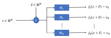
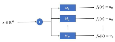
Figure 1: Conceptual framework of selective adversarial attack.

Figure 2: Conceptual framework of classification with multiple classifiers.

Consider some arbitrary input vector $x_{0}\in\mathbb{R}^{M}$, the corresponding true label $u_{0}\doteq f_{0}(x_{0})$, and an arbitrary set of $N$ “target labels” $\underline{u}_{t}\in\{1\dots L\}^{N}$. Note that if $x_{0}$ is chosen from the test distribution $p(x)$, then with high probability, all the $N$ classifiers produce the correct label to the unperturbed input vector $x_{0}$ i.e.

$$\Pr\left(\underline{f}(x_{0})=[u_{0}~{}u_{0}~{}\dots~{}u_{0}]\right) \approx 1$$ (3)

We now formally define an optimal selective adversarial attack as the smallest perturbation applied to the input vector $x_{0}$ that causes the $N$ classifiers $\mathcal{M}_{i},~{}i=1\dots N$ to output the target labels $\underline{u}_{t}$, each of which may be different from (or remains the same as) the true label $u_{0}$, and may be different from each other. Specifically the optimal selective perturbation $d(x_{0},\underline{u}_{t}):\mathbb{R}^{M}\times\{1\dots L\}^{N}\rightarrow\mathbb{R}^{M}$ for an input vector $x_{0}$ and the intended label set $\underline{u}_{t}$ is defined as:

$$d(x_{0},\underline{u}_{t}) \doteq\arg\min_{\delta\in\mathbb{R}^{M}}\lVert\delta\rVert,~{}$$

$$\mathrm{subject~{}to~{}} \underline{f}\left(x_{0}+\delta\right)\equiv\underline{u}_{t}$$ (4)

Remark. Note that in the definition (4), there is an implicit assumption that the constraint is feasible i.e. that there exists $x\in\mathbb{R}^{N}$ such that $\underline{f}(x)\equiv\underline{u}_{t}$ for any target label set $\underline{u}_{t}$. This, of course, is an assumption about the range of the functions $\underline{f}()$ describing the classifiers. Indeed it is a very strong assumption about how differently multiple nominally equivalent classifiers process their inputs. One of our objectives in this paper is to empirically test this assumption. Our findings in this paper surprisingly show that the constraint is often feasible under an arbitrary set of labels.

3.1 Selective Fooling

We now consider an interesting sub-class of selective adversarial attacks which we will call Selective Fooling. In this class of attacks, we choose a single adversarial target label $u_{a}$ that is different from the true label $u_{0}$ and design a perturbation that will cause a subset of $n<N$ classifiers in $\mathcal{M}$ to output the label $u_{a}$ while the remaining $N-n$ classifiers in $\mathcal{M}$ continue to output the true label $u_{0}$. In other words, we seek to selectively fool a subset of classifiers to output a particular target label $u_{a}$ while leaving the remaining ones unaffected.

Formally, Selective Fooling is a selective adversarial attack where the target label vector is set to be:

$$\underline{u}_{t}[i] =\begin{cases}&u_{a},~{}i\in\{1\dots n\},\\ &u_{0}~{}i\in\{n+1\dots N\}\end{cases}$$ (5)

for some $u_{a}\in\{1\dots L\}\setminus\{u_{0}\}$.

3.2 Selective Adversarial Attacks using Gradient Descent

We now discuss a simple method that extends previously known algorithms such as FGSM (Szegedy et al., 2013) that have been shown to be effective in generating adversarial examples to create selective adversarial perturbations. The basic idea is to formulate a cost function that serves as a proxy for the optimization problem in (4), and then use a gradient descent procedure to approximate a solution to (4).

Let $\mathbf{p}_{i}(x),~{}i=1\dots N,~{}x\in\mathbb{R}^{M}$ represent the probability distribution output by the classifier $M_{i}$ for the input vector $x$ over the $L$ possible labels $1\dots L$. Mathematically $\mathbf{p}_{i}(x)$ is a $1\times L$ vector that satisfies $\sum_{u=1}^{L}\mathbf{p}_{i,u}(x)\equiv 1,~{}\forall i,x$, where $\mathbf{p}_{i,u}(x)$ is the $u$-th element of $\mathbf{p}_{i}(x)$. In practice, $\mathbf{p}_{i}$ are typically calculated using a “softmax” function (Goodfellow et al., 2016) in the last layer of a deep neural network. Let $\mathbf{\delta}_{u},~{}u\in\{1\dots L\},$ be the $1\times L$ Kronecker delta vector i.e.:

$$\mathbf{\delta}_{u}[l] \doteq\begin{cases}1,&~{}l=u,\\ 0,~{}&\mathrm{otherwise}\end{cases}$$ (6)

Given a target label set $\underline{u}=[u_{1}~{}u_{2}~{}\dots~{}u_{N}]$, we define the following cost function $J(x),~{}x\in\mathbb{R}^{M}$:

$$J(x) =\sum_{i=1}^{N}\lVert\mathbf{p}_{i}(x)-\mathbf{\delta}_{u_{i}}\rVert^{2}$$ (7)

Our selective adversarial attack algorithm will iteratively reduce this proxy cost function by gradient descent. Of course a method for generating adversarial examples via gradient searches on the heuristic cost function in (7) can only approximate the optimal solution to (4). Indeed, we will see in our experimental results, that adversarial perturbations obtained from this cost function differs from the optimal solution in some interesting and counter-intuitive ways. We also remark that we can replace the cost function in (7) with other cost functions, such as cost functions using cross-entropy.

4 Experimental Results

We constructed a total of $N=5$ Convolutional Neural Networks with the architecture shown in Table 1. We trained each of them on the MNIST handwritten digit recognition dataset. All $N$ networks were identical except for a random initialization of their weights.

Layer name	Layer type
Input layer	input(28,28,1)
Layer 1	conv2d(32,3,3) + ReLU
Layer 2	conv2d(32,3,3) + ReLU + maxpool(2,2)
Layer 3	conv2d(64,3,3) + ReLU
Layer 4	conv2d(64,3,3) + ReLU + maxpool(2,2)
Layer 5	FC(200) + ReLU
Layer 6	FC(200) + ReLU
Layer 7	FC(10) + Softmax

Table 1: Architecture of neural networks in experiments. The FC is the fully connected layer, and the stride is 1 for convolution and maxpooling.

4.1 Training the Classifiers

We used a Stochastic Gradient Descent to minimize the softmax cross entropy function with a learning rate of $0.01$, a decay of $1e-6$, and a momentum of $0.9$ to train each of the $5$ networks. The models were trained using the MNIST training data, obtained from the Keras MNIST dataset, for $10$ epochs with $55,000$ images per epoch. The trained networks were evaluated on $10,000$ MNIST images from a separate test set. This resulted in all of the $5$ networks achieving an accuracy of at least $95\%$ accuracy on the test set. The models were trained using different random initializations of the network weight and bias parameters.

Next we describe the procedure we used to generate selective adversarial examples and a series of experiments that we performed using these trained networks.

4.2 Constructing Selective Adversarial Attacks

In all of our experiments, we used images with the true class label of ‘0’ (results for other digits are similar, and so we focus on label ‘0’ for our presentation ) from the aforementioned MNIST handwritten digit recognition dataset, and then constructed selective adversarial attacks designed to manipulate each of the $5$ networks in arbitrary pre-specified ways. We used modified versions of two popular algorithms to generate our adversarial examples: (a) the modified Carlini-Wagner (mCW) algorithm (Carlini & Wagner, 2017) and (b) the modified Fast Gradient Signed Method (mFGSM) (Szegedy et al., 2013; Kurakin et al., 2016).

The original Carlini-Wagner algorithm was designed to construct adversarial examples for a single classifier using a gradient descent procedure. We modified this algorithm to perform gradient descent on the loss function $J(x)$ as defined in (7). The following parameter values were used in our modified CW algorithm: confidence value $0.1$, learning rate $0.02$, the number of binary search steps $9$, and the max number of iterations $10,000$. Our modified FGSM algorithm also used the loss function very similar to (7) (with the cross-entropy function replacing the $l_{2}$ norm in (7)). In our experiments with the modified FGSM algorithm, we set the parameter $\epsilon=0.075$ with the maximum number of iterations fixed at $30$.

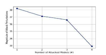
Figure 3: Average size of the adversarial perturbations generated by the mCW algorithm as a function of the number of attacked classifiers.

Figure 4: Average size of the mFGSM attack as a function of the number of attacked classifiers.

4.3 Selective Fooling Experiment with Two Classifiers

Our first set of experiments involved the simple sub-class of selective adversarial attacks defined in Section 3.1 with $N=2,~{}n=1$ i.e. we attempt to construct adversarial examples that successfully fool one of two classifiers while leaving the other classifier unaffected.

A total of $25$ images of the label $0$ were perturbed using both the mCW and mFGSM algorithms described earlier with random target labels. The mFGSM algorithm was able to successfully construct Selective Fooling attacks on all of the $25$ images. The mCW algorithm was also able to generate adversarial examples for a majority of images, but takes longer to converge than mFGSM.

This shows the existence of selective adversarial examples, at least for this simple special case of Selective Fooling attack, and suggests that it may indeed be feasible to construct adversarial examples that affect multiple classifiers in different ways (and surprisingly often in all the possible ways) and motivates a deeper study of selective adversarial attacks.

We also tested the effect of the adversarial examples generated by the mCW algorithm on a third classifier that was not involved in the construction of the attack; the confidence value of this third classifier in the true label ($0$) averaged over the $25$ images was calculated to be $0.778$. Roughly speaking, this shows that on average, a third classifier is approximately $75\%$ unaffected by the Selective Fooling attack. In contrast, the corresponding number for a non-selective fooling attack against just one classifier using the unmodified Carlini-Wagner algorithm was $0.843$ i.e. a third classifier was approximately $85\%$ unaffected by such a non-selective fooling attack. This seems somewhat counter-intuitive: we may expect that a selective attack that narrowly targets one classifier while leaving another classifier unaffected will be less likely to affect a third classifier. Below we consider a possible explanation for this and certain other similarly counter-intuitive results.

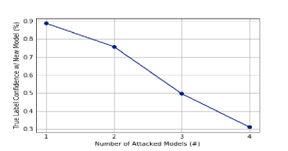
Figure 5: Confidence value in the true label for a fifth classifier as a function of the number of attacked classifiers.

Figure 6: Magnitude of the FGSM attack as the number of attacked models increases and the number of defended model decreases when observing the general $M$ and $n$ attacks for four total models.

4.4 Selective Fooling Experiment with Four Classifiers

1. One Attacked, Three Defended
   

2. Two Attacked, Two Defended
   

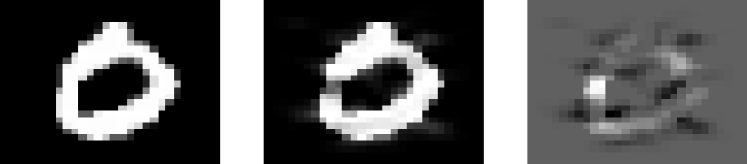
3. Three Attacked, One Defended
   

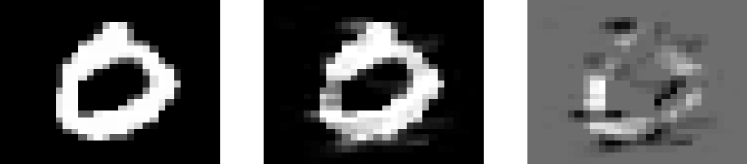
4. Four Attacked, None Defended
   

Figure 7: Examples of input images, their adversarial counterpart, and the perturbations added for cases where a) $n$=1, b) $n$=2, c) $n$=3, and d) $n$=4 classifiers are attacked via the mCW algorithm out of $N=4$ total.

In our next set of experiments, we constructed a series of Selective Fooling attacks with $N=4$ classifiers. Specifically, for a set of $25$ images with the true label of $u_{0}=0$ and for each of the $15$ non-empty subsets of the $4$ classifiers, we attempted to construct selective adversarial attacks to drive their outputs to a target label of $u_{a}=9$ using both the mCW and mFGSM algorithms. Surprisingly, both the mCW and mFGSM methods were able to successfully construct adversarial examples that successfully fooled each of the $2^{4}-1=15$ non-empty subsets of the $N=4$ classifiers while keeping the complementary subset of classifiers unfooled, for each of the $25$ images.

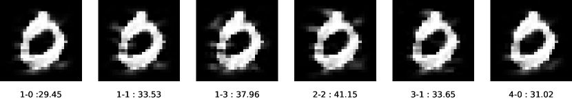
Figure 8: For an adversarial image attacking $m=N-n$ classifiers and defending $n$ classifiers, designated as $m-n$, we can see the magnitudes of the attacks for the unmodified Carlini-Wagner attack (1-0), the simplest attack and defend case (1-1), and the four subset cases (where the target labels are all set to $9$).

The average size of the perturbations measured as the sum of the absolute value of pixel differences between the input image and the adversarial image, is shown as a function of the number of targeted classifiers $n$ in Figs. 4 and 4 for the mCW and mFGSM algorithms respectively.

Discussion. The mere fact that there exists small perturbations which selectively and precisely attack every possible subset of classifiers is quite surprising. This suggests that these classifiers might look at very different features for classifications, and do not “think” alike, even though they share the same architectures and training data. Figures 4 and 4 suggest that on average we need smaller perturbations to attack more classifiers. We might expect that it would take larger perturbations to simultaneously change the outputs of two classifiers compared to one classifier. One possible explanation for this observation - as well as our earlier observation about transferability of the Selective Fooling attack - is that the attacks generated by the mCW and mFGSM algorithms are not close to being optimal; a search constrained to leave one or more classifiers unaffected leads to smaller perturbation perhaps because it is forced to keep more features of the original image intact as compared to an unconstrained search.

The confidence in the true label from a fifth classifier that was not involved in the generation of the adversarial examples is shown as a function of the size of the target set $n$ in Figure 6 for the mCW generated attacks. This plot is consistent with our intuitive expectation that an adversarial example that successfully attacks many classifiers simultaneously is also more statistically likely to transfer to a random classifier.

Adversarial example images for different values of $n$ are shown in Figure 7. Typical examples of adversarial images with varying $N$ and $n$ and their respective magnitudes can be seen in Fig. 8.

4.5 Attacking and Defending Subsets of Four Classifiers with Different Target Labels

Our final set of experiments involved a generalization of the Selected Fooling attack where a subset $n$ of $N=4$ classifiers were targeted to be attacked to $n$ different target labels chosen at random, while keeping the outputs of the remaining $N-n$ classifiers unchanged. Once again, the mFSGM algorithm was able to successfully generate adversarial examples for all $15$ non-empty subsets of the $N=4$ classifiers. The average size of the resulting perturbations as a function of $n$ is shown in Fig. 6.

5 Conclusions

We formulated the problem of selective adversarial attacks, and presented an experimental investigation of a generalized class of adversarial attacks that are designed to manipulate the outputs of multiple machine learning classifiers simultaneously in arbitrarily pre-defined ways. We formulated a novel optimization problem to search for such selective attacks, and applied modified versions of popular algorithms used for the construction of white-box adversarial examples to design targeted attacks on $5$ different trained classifiers for the MNIST dataset. Our results show that it is indeed possible to construct precisely targeted adversarial attacks that can arbitrarily modify the outputs of multiple classifiers while keeping another set of classifiers unaffected. These results motivate a deeper study of such selective adversarial attacks and also suggest that different classifiers that have nominally similar performance may in fact have very different decision regions.

References

- Adam et al. (2019) Adam, G., Smirnov, P., Haibe-Kains, B., and Goldenberg, A. Reducing adversarial example transferability using gradient regularization. arXiv:1904.07980 [cs.LG], April 2019.
- Bhambri et al. (2019) Bhambri, S., Muku, S., Tulasi, A., and Buduru, A. A study of black box adversarial attacks in computer cision. arXiv:1912.01667 [cs, stat], December 2019. arXiv: 1912.01667.
- Bose et al. (2019) Bose, A., Cianflone, A., and Hamiltion, W. Generalizable adversarial attacks using generative models. arXiv:1905.10864 [cs, stat], May 2019. arXiv: 1905.10864.
- Brunner et al. (2018) Brunner, T., Diehl, F., Le, M., and Knoll, A. Guessing smart: biased sampling for efficient black-box adversarial attacks. arXiv:1812.09803 [cs, stat], December 2018. arXiv: 1812.09803.
- Carlini & Wagner (2017) Carlini, N. and Wagner, D. Towards evaluating the robustness of neural networks. In 2017 IEEE Symposium on Security and Privacy (SP), pp. 39–57, May 2017. doi: 10.1109/SP.2017.49.
- Carlini & Wagner (2018) Carlini, N. and Wagner, D. Audio adversarial examples: targeted attacks on speech-to-text. arXiv:1801.01944 [cs], January 2018. arXiv: 1801.01944.
- Chen et al. (2017) Chen, P., Zhang, H., Sharma, Y., Yi, J., and Hsieh, C. ZOO: zeroth order optimization based black-box attacks to deep neural networks without training substitute models. Proceedings of the 10th ACM Workshop on Artificial Intelligence and Security - AISec ’17, pp. 15–26, 2017. doi: 10.1145/3128572.3140448. arXiv: 1708.03999.
- Dong et al. (2019) Dong, Y., Pang, T., Su, H., and Zhu, J. Evading defenses to transferable adversarial examples by translation-invariant attacks. arXiv:1904.02884 [cs.CV], April 2019.
- Fawzi et al. (2018) Fawzi, A., Fawzi, H., and Fawzi, O. Adversarial vulnerability for any classifier. arXiv:1802.08686 [cs, stat], February 2018. arXiv: 1802.08686.
- Goodfellow et al. (2014) Goodfellow, I., Shlens, J., and Szegedy, C. Explaining and harnessing adversarial examples. arXiv:1412.6572 [cs, stat], December 2014. arXiv: 1412.6572.
- Goodfellow et al. (2016) Goodfellow, I., Bengio, Y., Courville, A., and Bengio, Y. Deep learning, volume 1. MIT press Cambridge, 2016.
- Grosse et al. (2016) Grosse, K., Papernot, N., Manoharan, P., Backes, M., and McDaniel, P. Adversarial perturbations against deep neural networks for malware classification. arXiv:1606.04435 [cs], June 2016. arXiv: 1606.04435.
- Ilyas et al. (2017) Ilyas, A., Jalal, A., Asteri, E., Daskalakis, C., and Dimakis, A. The robust manifold defense: adversarial training using generative models. arXiv:1712.09196 [cs, stat], December 2017. arXiv: 1712.09196.
- Ilyas et al. (2018) Ilyas, A., Engstrom, L., Athalye, A., and Lin, J. Black-box adversarial attacks with limited queries and information. arXiv:1804.08598 [cs, stat], July 2018. arXiv: 1804.08598.
- Kang et al. (2019) Kang, D., Sun, Y., Brown, T., Hendrycks, D., and Steinhardt, J. Transfer of adversarial robustness between perturbation types. arXiv:1905.01034 [cs, stat], May 2019. arXiv: 1905.01034.
- Khormali et al. (2019) Khormali, A., Abusnaina, A., Chen, S., Nyang, D., and Mohaisen, A. COPYCAT: practical adversarial attacks on visualization-based malware detection. arXiv:1909.09735 [cs], September 2019. arXiv: 1909.09735.
- Ko et al. (2019) Ko, C., Lyu, Z., Weng, T., Daniel, L., Wong, N., and Lin, D. POPQORN: quantifying robustness of recurrent neural networks. arXiv:1905.07387 [cs, stat], May 2019. arXiv: 1905.07387.
- Kurakin et al. (2016) Kurakin, A., Goodfellow, I., and Bengio, S. Adversarial examples in the physical world. arXiv:1607.02533 [cs.CV], July 2016.
- Li et al. (2019) Li, F., Lai, L., and Cui, S. On the adversarial robustness of subspace learning. arXiv:1908.06210 [cs, eess, stat], August 2019. arXiv: 1908.06210.
- Lin et al. (2019) Lin, J., Song, C., He, K., Wang, L., and Hopcroft, J. Nesterov accelerated gradient and scale invariance for improving transferability of adversarial examples. arXiv:1908.06281 [cs, stat], August 2019. arXiv: 1908.06281.
- Liu et al. (2016) Liu, Y., Chen, X., Liu, C., and Song, D. Delving into transferable adversarial examples and black-box attacks. arXiv:1611.02770 [cs], November 2016. arXiv: 1611.02770.
- Madry et al. (2017) Madry, A., Makelov, A., Schmidt, L., Tsipras, D., and Vladu, A. Towards deep learning models resistant to adversarial attacks. arXiv:1706.06083 [cs, stat], June 2017. arXiv: 1706.06083.
- Meng et al. (2020) Meng, Y., Su, J., O’Kane, J., and Jamshidi, P. Ensembles of many diverse weak defenses can be strong: defending deep neural networks against adversarial attacks. arXiv:2001.00308 [cs, stat], January 2020. arXiv: 2001.00308.
- Meunier et al. (2019) Meunier, L., Atif, J., and Teytaud, O. Yet another but more efficient black-box adversarial attack: tiling and evolution strategies. arXiv:1910.02244 [cs], October 2019. arXiv: 1910.02244.
- Moosavi-Dezfooli et al. (2016) Moosavi-Dezfooli, S., Fawzi, A., and Frossard, P. DeepFool: a simple and accurate method to fool deep neural networks. pp. 2574–2582, 2016.
- Narodytska & Kasiviswanathan (2016) Narodytska, N. and Kasiviswanathan, S. Simple black-box adversarial perturbations for deep networks. arXiv:1612.06299 [cs, stat], December 2016. arXiv: 1612.06299.
- Papernot et al. (2017) Papernot, N., McDaniel, P., Goodfellow, I., Jha, S., Celik, Z., and Swami, A. Practical black-box attacks against machine learning. In Proceedings of the 2017 ACM on Asia Conference on Computer and Communications Security, ASIA CCS ’17, pp. 506–519, New York, NY, USA, 2017. ACM.
- Samangouei et al. (2018) Samangouei, P., Kabkab, M., and Chellappa, R. Defense-GAN: protecting classifiers against adversarial attacks using generative models. arXiv:1805.06605 [cs, stat], May 2018. arXiv: 1805.06605.
- Song et al. (2018) Song, Y., Kim, T., Nowozin, S., Ermon, S., and Kushman, N. PixelDefend: leveraging generative models to understand and defend against adversarial examples. arXiv:1710.10766 [cs], May 2018. arXiv: 1710.10766.
- Szegedy et al. (2013) Szegedy, C., Zaremba, W., Sutskever, I., Bruna, J., Erhan, D., Goodfellow, I., and Fergus, R. Intriguing properties of neural networks. arXiv:1312.6199 [cs], December 2013. arXiv: 1312.6199.
- Tramer et al. (2017) Tramer, F., Papernot, N., Goodfellow, I., Boneh, D., and McDaniel, P. The space of transferable adversarial examples. arXiv:1704.03453 [cs, stat], April 2017. arXiv: 1704.03453.
- Tu et al. (2019) Tu, C., Ting, P., Chen, P., Liu, ., Zhang, H., Yi, J., Hsieh, C., and Cheng, S. AutoZOOM: autoencoder-based zeroth order optimization method for attacking black-box neural networks. Proceedings of the AAAI Conference on Artificial Intelligence, 33(01):742–749, July 2019. ISSN 2374-3468. doi: 10.1609/aaai.v33i01.3301742.
- Wang et al. (2020) Wang, S., Nepal, S., Rudolph, C., Grobler, M., Chen, S., and Chen, T. Backdoor attacks against transfer learning with pre-trained deep learning models. arXiv:2001.03274 [cs], January 2020. arXiv: 2001.03274.
- Xie et al. (2018) Xie, C., Wu, Y., van der Maaten, L., Yuille, A., and He, K. Feature denoising for improving adversarial robustness. arXiv:1812.03411 [cs.CV], December 2018.
- Yan et al. (2019) Yan, Z., Guo, Y., and Zhang, C. Subspace attack: exploiting promising subspaces for query-efficient black-box attacks. arXiv:1906.04392 [cs], June 2019. arXiv: 1906.04392.
- Yi et al. (2019) Yi, J., Xie, H., Zhou, L., Wu, X., Xu, W., and Mudumbai, R. Trust but verify: an information-theoretic explanation for the adversarial fragility of machine learning systems, and a general defense against adversarial attacks. arXiv:1905.11381 [cs, stat], May 2019. arXiv: 1905.11381.
- Yin et al. (2019) Yin, X., Kolouri, S., and Rohde, G. Divide-and-conquer adversarial detection. arXiv:1905.11475 [cs, stat], May 2019. arXiv: 1905.11475.
- Zhang & Liang (2019) Zhang, Y. and Liang, P. Defending against whitebox adversarial attacks via randomized discretization. arXiv:1903.10586 [cs, stat], March 2019. arXiv: 1903.10586.
- Zhao et al. (2019) Zhao, Y., Shumailov, I., Cui, H., Gao, X., Mullins, R., and Anderson, R. Blackbox attacks on reinforcement learning agents using approximated temporal information. arXiv:1909.02918 [cs, stat], September 2019. arXiv: 1909.02918.
- Zheng et al. (2019) Zheng, H., Zhang, Z., Gu, J., Lee, H., and Prakash, A. Efficient adversarial training with transferable adversarial examples. arXiv:1912.11969 [cs], December 2019. arXiv: 1912.11969.
- Zhou et al. (2019) Zhou, Z., Guan, H., Bhat, M., and Hsu, J. Fake news detection via NLP is vulnerable to adversarial attacks. arXiv:1901.09657 [cs], January 2019. arXiv: 1901.09657.
- Zügner & Günnemann (2019) Zügner, D. and Günnemann, S. Adversarial attacks on graph neural networks via meta Learning. arXiv:1902.08412 [cs, stat], February 2019. arXiv: 1902.08412.