Neural Network-based Top Tagger with Two-Point Energy Correlations and Geometry of Soft Emissions

Abstract

Deep neural networks trained on jet images have been successful in classifying different kinds of jets. In this paper, we identify the crucial physics features that could reproduce the classification performance of the convolutional neural network in the top jet vs. QCD jet classification. We design a neural network that considers two types of substructural features: two-point energy correlations, and the IRC unsafe counting variables of a morphological analysis of jet images. The new set of IRC unsafe variables can be described by Minkowski functionals from integral geometry. To integrate these features into a single framework, we reintroduce two-point energy correlations in terms of a graph neural network and provide the other features to the network afterward. The network shows a comparable classification performance to the convolutional neural network. Since both networks are using IRC unsafe features at some level, the results based on simulations are often dependent on the event generator choice. We compare the classification results of Pythia 8 and Herwig 7, and a simple reweighting on the distribution of IRC unsafe features reduces the difference between the results from the two simulations.

1 Introduction

Interest in deep learning in collider physics Larkoski:2017jix ; Asquith:2018igt ; Guest:2018yhq ; Radovic:2018dip ; Abdughani:2019wuv has been growing in recent years. Many applications of deep learning have appeared in jet classification Almeida:2015jua ; deOliveira:2015xxd ; Komiske:2016rsd ; Butter:2017cot ; Dery:2017fap ; Kasieczka:2017nvn ; Louppe:2017ipp ; Cheng:2017rdo ; Egan:2017ojy ; Metodiev:2017vrx ; Komiske:2018cqr ; Macaluso:2018tck ; Andreassen:2018apy ; Lim:2018toa ; Qu:2019gqs ; Chakraborty:2019imr ; Andreassen:2019txo ; Chen:2019uar ; Cheng:2019isq ; Chen:2019apv ; Kasieczka:2020yyl , anomaly detection Heimel:2018mkt ; Farina:2018fyg ; Hajer:2018kqm ; Dillon:2019cqt ; Diefenbacher:2019ezd ; Blance:2019ibf ; Roy:2019jae ; Collins:2019jip ; Amram:2020ykb ; Nachman:2020lpy ; Andreassen:2020nkr , particle identification Guest:2016iqz ; ATL-PHYS-PUB-2017-003 ; CMS-DP-2017-005 , pileup mitigation Martinez:2018fwc ; Komiske:2017ubm ; Komiske:2018lor , event generation Bendavid:2017zhk ; Klimek:2018mza ; Otten:2019hhl ; Hashemi:2019fkn ; DiSipio:2019imz ; Butter:2019cae ; Carrazza:2019cnt ; SHiP:2019gcl ; Butter:2019eyo ; Bishara:2019iwh ; Bothmann:2020ywa ; Gao:2020vdv ; Gao:2020zvv ; Matchev:2020tbw ; Badger:2020uow , unfolding Andreassen:2019cjw ; Bellagente:2019uyp , and parton distribution functions Forte:2002fg ; Forte:2002us ; Rojo:2004iq ; DelDebbio:2004xtd ; DelDebbio:2007ee ; Ball:2008by ; Ball:2009mk ; Ball:2010de ; Ball:2010gb ; Ball:2011mu ; Lionetti:2011pw ; Ball:2012cx ; Ball:2013hta ; Carrazza:2013bra ; Carrazza:2013wua ; Ball:2014uwa ; Ball:2017nwa ; Bertone:2017tyb . Deep learning will be used more in the analysis of LHC run III data. Among those, jet classification using neural networks is one of the well-established areas. Several approaches have been proposed, and the performance of different models has been compared Kasieczka:2019dbj . For the classification between top jets and QCD jets, neural networks trained on low-level inputs showed a significant improvement in the classification performance compared to the previous methods Aaboud:2018psm .

Before the deep learning in jet classification, the classification using the jet substructure information achieved remarkable success. The particles coming from the decay of a boosted heavy particle give clear substructures inside the reconstructed jet. The substructure maybe characterized by various manners; for example, by going through the jet clustering sequence Butterworth:2008iy ; Thaler:2008ju ; Kaplan:2008ie ; Ellis:2009su ; CMS:2009lxa ; Plehn:2009rk ; Plehn:2010st ; Dasgupta:2013ihk ; Larkoski:2014wba , reclustering jet constituents into the jets with smaller radius to identify subjets Butterworth:2008iy ; Krohn:2009th ; Soper:2011cr ; Soper:2012pb ; Soper:2014rya , or the energy correlations Tkachov:1995kk ; Thaler:2010tr ; Jankowiak:2011qa ; Jankowiak:2012na ; Larkoski:2012eh ; Gallicchio:2012ez ; Larkoski:2013eya ; Larkoski:2014gra ; Moult:2016cvt ; Komiske:2017aww ; Chen:2019bpb . Note that such substructures are often defined by infrared and collinear (IRC) safe algorithms or observables which are theoretically more predictable. The IRC unsafe quantities are also used in the jet classification. For example, the number of charged tracks Gallicchio:2012ez is very useful quantity for the quark jet vs. gluon jet classification. In some cases, the IRC unsafe counting variable has an IRC safe counterpart such as soft drop multiplicity Frye:2017yrw .

The pattern of soft radiation is also important for the classification. For example, a color singlet boosted heavy particle has emission isolated in terms of soft activity unlike quark and gluon jets. The related substructure quantity has been incorporated in Higgs taggers Gallicchio:2010sw ; Gallicchio:2010dq and top taggers Hook:2011cq . Such soft particle distribution may also contribute to the jet classification using neural networks in order to improve the performance.

While the improvement using deep learning is impressive, the physics behind it has not been addressed. So far, the classifier based on a convolutional neural network (CNN) trained on the jet image performs well for selecting the top jets. It is numerically shown that the CNN uses IRC safe features mostly Choi:2018dag , but it is not easy to make an estimate of systematic uncertainties from various sources without knowing what kind of features of the jet is used in the model. Bayesian networks are capable of tracking those uncertainties Bollweg:2019skg ; Kasieczka:2020vlh , but it is also useful to identify the features in order to interpret the network outputs and uncertainties. The aim of this paper is to provide a convenient parametrization of the jet feature contributing to the classification using jet images.

In this paper, we address the question in the following steps. In section 2, we first introduce a graph neural network 1555942 ; 4700287 ; DBLP:journals/corr/RaposoSBPLB17 ; NIPS2017_7082 ; DBLP:journals/corr/abs-1806-01261 with constraints, and the network is more restrictive than CNN. Graph networks are flexible enough for analyzing multiple objects appears at the LHC, and have been studied in various contexts Henrion2017NeuralMP ; Martinez:2018fwc ; Komiske:2018cqr ; Qu:2019gqs ; Chen:2019apv ; Qasim:2019otl ; Abdughani:2018wrw ; Moreno:2019bmu ; Moreno:2019neq ; Ren:2019xhp ; Mikuni:2020wpr ; Bister:2020rfv . The graph network in this paper has access to only IRC safe two-point energy correlations Basham:1978bw ; Basham:1978zq ; Basham:1979zw ; Basham:1979gh ; Jankowiak:2011qa ; Jankowiak:2012na ; Larkoski:2012eh ; Lim:2018toa ; Chakraborty:2019imr . It was shown that the network has comparable performance to the CNN in the Higgs jet vs. QCD jet classification Chakraborty:2019imr . We use this network for top jet vs. QCD jet classification, and it is a good starting point toward the network whose top tagging performance is comparable to the CNN.

To integrate the IRC unsafe quantities to this framework, we formulate a sequence of novel morphological measures based on Minkowski functionals, in section 3. The sequence includes the number of pixels with finite energy deposit (active pixels), $N^{(0)}$, the number of pixels that touch the active pixels, $N^{(1)}$. These numbers can be considered as a discretized version of Minkowski functionals. They are formulated in a mathematical theory called integral geometry and describes geometric measures to the point distributions. The application of the Minkowski functionals has already been considered in the astrophysical analysis Mecke:1994ax ; Schmalzing:1995qn ; Schmalzing:1997aj ; Schmalzing:1997uc ; WINITZKI199875 ; Kerscher:2001ec ; Beisbart:2001gk ; Matsubara_2003 ; Hikage:2006fe ; G_ring_2013 ; klatt2017morphometric2 ; klatt2017morphometric3 ; Chingangbam:2017sap ; Pranav:2018pnu , and statistical mechanics PhysRevE.53.4794 ; 10.1007/3-540-45043-2_6 ; Mantz_2008 . We perform a morphological analysis to the distribution of soft activity in the jet.

When the first few elements of the Minkowski sequence are included in the graph network inputs, the new classifier has the same performance as the jet image CNN classifier, as shown in section 4. This means that the improvement of the CNN classifier comes from the geometric quantities of the pixels, and also it is summarized by just a few numbers of additional variables. Our result suggests that the CNN output is correlated to a few numbers of geometric quantities derived from the jet image.

In the collider study, event simulators are used extensively to estimate the signal and background distributions. The sequence of Minkowski functionals calculated from a jet image is IRC unsafe quantities, and the simulated data need to be calibrated by the experimental data. We propose an event reweighting method based on the IRC unsafe quantities for the calibration in section 5. We conclude in section 6.

2 IRC Safe Two-Point Energy Correlations and Relation Network

The jet classifier using a deep learning model trained on the jet image has achieved better performance compared with the other statistical methods. Still, it is not straightforward to identify the key physical features that contributed to the improvement, other than looking for the hidden data representations of the CNN deOliveira:2015xxd ; Kasieczka:2017nvn ; Lin:2018cin ; Farina:2018fyg , or checking the response of the network after perturbing the inputs Choi:2018dag . Note that organized networks whose hidden representations have physical interpretations Butter:2017cot ; Andreassen:2018apy ; Komiske:2018cqr ; Chakraborty:2019imr ; Cheng:2019isq allow us to interpret the results in terms of physics. For this purpose, we consider flexible and interpretable quantities derived from the jet image and use them as inputs to a jet classifier modeled by a multilayer perceptron (MLP). Additional inputs are considered until the performance of the classifier is equivalent to that of the best classifiers using the jet image.

We first introduce two-point energy correlation spectra $S_{2}$ Lim:2018toa ; Chakraborty:2019imr as a function of the distance between the jet constituents $R$,

$$S_{2,\mathbf{J}_{a}\mathbf{J}_{b}}(R) = S_{2,ab}(R)=\int d\vec{R}_{1}d\vec{R}_{2}\,P_{T,\mathbf{J}_{a}}(\vec{R}_{1})P_{T,\mathbf{J}_{b}}(\vec{R}_{2})\,\delta(R-R_{12}),$$ (1)

$$S_{2}(R) = S_{2,\mathbf{J}\mathbf{J}}(R),$$ (2)

where $S_{2,ab}$ is a shorthand notation of $S_{2,\mathbf{J}_{a}\mathbf{J}_{b}}$;

$$P_{T,\mathbf{J}_{a}}(\vec{R})=\sum_{i\in\mathbf{J}_{a}}p_{T,i}\,\delta(\vec{R}-\vec{R}_{i}),$$ (3)

is an energy flow of a subjet $\mathbf{J}_{a}$ of a jet $\mathbf{J}$; $a$ and $b$ are indices of the subjet. The $R_{ij}$ is the relative angular distance between two constituents, $\sqrt{(\eta_{i}-\eta_{j})^{2}+(\phi_{i}-\phi_{j})^{2}}$. The $S_{2,ab}$ is an IRC safe quantity. For the Higgs jet vs. QCD jet classification, an MLP trained on the transverse momenta, masses, and $S_{2}$’s of the jet and trimmed jet performs nearly as good as a CNN trained on jet images. In Chakraborty:2019imr , we relate $S_{2,ab}$ to the generic jet classifiers through its formal expansion with respect to the energy flow. This shows that $S_{2,ab}$ is flexible enough to describe many quantities for the classification of jets.

In this section, we first derive $S_{2,ab}$ in terms of a vertex-labeled fully-connected graph to integrate them into a framework of the graph network and extend it for further ML analysis. A graph is a set of the points and the lines connecting them, which are called vertices and edges, respectively. In our setup, each vertex of the graph corresponds to a jet constituent, and the inputs to the $i$-th vertex are the jet constituent momentum $p_{i}$. The labels of a vertex denote the subjets to which the constituent $i$ belongs. The graph network also has the other inputs $\bm{u}$ calculated from the given jet, for example, (sub)jet transverse momentum and mass. A schematic diagram of the graph is in figure 1. Each circle represents the jet constituent assigned to the corresponding vertex. The dot-dashed lines are the edges.

Figure 1: A schematic diagram of the graph representation of a jet used in this paper. Each vertex corresponds to a jet constituent, and a line between two circles represents the variable calculated from the two vertices. Each dashed rectangle represents a subjet that contains the enclosed jet constituents.

(a)

(b)

(c)

Figure 2: Schematic diagrams of the graph representations of jets. (a) and (b) are top jet images, and (c) is a QCD jet image. Lines represent the graphs on the jet images. The red solid lines are edges between the constituents of the trimmed jet $\mathbf{J}_{\mathrm{trim}}$. The green dashed lines are the edges between the constituents of $\mathbf{J}_{\mathrm{trim}}$ and the constituents of $\mathbf{J}\setminus\mathbf{J}_{\mathrm{trim}}$. The blue dot-dashed lines are edges between the constituents of $\mathbf{J}\setminus\mathbf{J}_{\mathrm{trim}}$. Note that we omitted some edges for readability.

We use a kind of graph network called a relation network (RN) DBLP:journals/corr/RaposoSBPLB17 ; NIPS2017_7082 that mainly utilizes correlations between two vertices. The reason for using this network is that the kernel of the parton shower model is 1 $\rightarrow$ 2 splitting of partons. The classifier can focus on the two-point correlations by using the relation network as a functional model. The classifier output $\bm{u}^{\prime}$ is the value of a functional model $\phi^{u}$ applied to the edge outputs $\bar{\bm{e}}_{ab}$, the vertex outputs $\bar{p}_{a}$, and the predefined inputs $\bm{u}$.

$$\bm{u}^{\prime}=\phi^{u}\left(\bar{\bm{e}}_{ab},\bar{\bm{p}}_{a},\bm{u}\right).$$ (4)

The edge output $\bar{\bm{e}}_{ab}$ is the aggregated two-point correlation between $\mathbf{J}_{a}$ and $\mathbf{J}_{b}$,

$$\bar{\bm{e}}_{ab} = \sum_{\begin{subarray}{c}i\in\mathbf{J}_{a}\\ j\in\mathbf{J}_{b}\end{subarray}}\phi^{e}_{ab}(p_{i},p_{j},\bm{u}),$$ (5)

where $\phi^{e}_{ab}(p_{i},p_{j},\bm{u})$ is a functional model of a two-point correlation assigned on edge linking two jet constituents $i$ and $j$. The vertex output $\bar{\bm{p}}_{a}$ is the aggregated one-point correlation of $\mathbf{J}_{a}$,

$$\quad\bar{\bm{p}}_{a}=\sum_{i\in\mathbf{J}_{a}}\phi^{v}_{a}(p_{i},\bm{u}),$$ (6)

where $\phi^{v}_{a}(p_{i},\bm{u})$ is a functional model of a one-point correlation assigned to a vertex that corresponds to a jet constituent $i$. The correlations $\bar{\bm{p}}_{a}$ and $\bar{\bm{e}}_{ab}$ are symmetric for the permutation of the jet constituents. We train $\bm{u}^{\prime}$ to be the logits for the classification.

We use energy correlators Tkachov:1995kk ; Komiske:2017aww for $\phi^{e}$ and $\phi^{v}$ to restrict $\bm{u}^{\prime}$ to be IRC safe. Namely, we consider the following IRC safe $C$-correlators for $\bar{\bm{p}}_{a}$ and $\bar{\bm{e}}_{ab}$,

$$\bar{\bm{p}}_{a} = \sum_{i\in\mathbf{J}_{a}}p_{T,i}w_{a}(\vec{R}_{i};\bm{u})\rightarrow p_{T,\mathbf{J}_{a}}w_{a}(\bm{u}),$$ (7)

$$\bar{\bm{e}}_{ab} = \sum_{\begin{subarray}{c}i\in\mathbf{J}_{a}\\ j\in\mathbf{J}_{b}\end{subarray}}p_{T,i}p_{T,j}w_{ab}(\vec{R}_{i},\vec{R}_{j};\bm{u})\rightarrow\sum_{i\in\mathbf{J}_{a}}\sum_{j\in\mathbf{J}_{b}}p_{T,i}p_{T,j}w_{ab}(R_{ij};\bm{u}),$$ (8)

where $p_{T,i}$ is the transverse momentum of the $i$-th constituent, $\vec{R}_{i}=(\eta_{i},\phi_{i})$ is the pseudorapidity-azimuthal coordinate of the $i$-th constituent. The functions $w_{a}$ and $w_{ab}$ are the angular weighting functions of one-point and two-point energy correlators, respectively. The last step of the equation comes from the assumption that the classifier does not depend on the absolute angular coordinates of the (sub)jet constituents but uses the relative angular distances.

The last expression in eq. (8) can be written in terms of an integral Lim:2018toa ,

$$\bar{\bm{e}}_{ab}=\int dR\,S_{2,ab}(R)w_{ab}(R,\bm{u}).$$ (9)

We may absorb the angular weighting functions $w_{ab}$ to $\phi^{u}$ so that the $S_{2,ab}$ and $p_{T,\mathbf{J}_{a}}$ can be considered as effective inputs to the network.

$$\bm{u}^{\prime}=\phi^{u}\left(S_{2,ab}(R),p_{T,\mathbf{J}_{a}},\bm{u}\right).$$ (10)

This setup is equivalent to the one using $S_{2,ab}$ as input, discussed in Lim:2018toa .

We now design a top tagger based on eq. (10). The structure of the graph is specified by the subjet label $a$ and $b$ of $S_{2,ab}$. We consider the following subjet labels for the top jet vs. QCD jet classification.

• the trimmed jet, $\mathbf{J}_{\mathrm{trim}}$, denoted by $h$,

• the compliment set of $\mathbf{J}_{\mathrm{trim}}$, $\mathbf{J}\setminus\mathbf{J}_{\mathrm{trim}}$, denoted by $s$,

• the leading $p_{T}$ subjet, $\mathbf{J}_{\mathrm{1}}$, denoted by $1$,

• the compliment set of $\mathbf{J}_{\mathrm{1}}$, $\mathbf{J}\setminus\mathbf{J}_{\mathrm{1}}$, denoted by $c$,

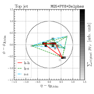
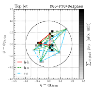
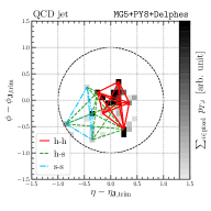
Examples of the vertex-labeled graphs are in figure 2. Note that the following relations hold for $S_{2}$ and $S_{2,ab}$,

$$S_{2}(R) = S_{2,hh}(R)+2S_{2,hs}(R)+S_{2,ss}(R),$$ (11)

$$= S_{2,11}(R)+2S_{2,1c}(R)+S_{2,cc}(R).$$ (12)

Because $S_{2,ss}$ contains only the correlations between soft constituents, which is theoretically unpredictable and less reliable experimentally, we define the following combinations as in Lim:2018toa .

$$S_{2,\mathrm{trim}}(R) = S_{2,hh}(R),$$ (13)

$$S_{2,\mathrm{soft}}(R) = 2S_{2,hs}(R)+S_{2,ss}(R).$$ (14)

The $S_{2,\mathrm{trim}}$ and $S_{2,\mathrm{soft}}$ distributions of the top jets and QCD jets in figure 2 are shown in figure 3.

In parton level, $S_{2,\mathrm{trim}}$ and $S_{2,\mathrm{soft}}$ of a top quark have up to four peaks of delta functions and written as follows if all partons are sufficiently high $p_{T}$.

$$S_{2,\mathrm{trim}}(R) = (p_{T,b}^{2}+p_{T,q}^{2}+p_{T,\bar{q}}^{2})\,\delta(R)$$ (15)

$$\vphantom{1}+2p_{T,b}p_{T,q}\delta(R-R_{bq})+2p_{T,b}p_{T,\bar{q}}\delta(R-R_{b\bar{q}})+2p_{T,q}p_{T,\bar{q}}\delta(R-R_{q\bar{q}}),$$

$$S_{2,\mathrm{soft}}(R) = 0.$$ (16)

Here, $b$ is a bottom quark from a top quark decay, and $q$ and $\bar{q}$ are quarks from the subsequent $W$ boson decay. Figure 3(a) is the $S_{2,\mathrm{trim}}$ of the top jet that has those four peaks clearly. This pattern is relatively rare for QCD jets. Figure 3(c) is the $S_{2,\mathrm{trim}}$ of a typical QCD jet.

In the case where the characteristic angular scales of the top quark, $R_{bq}$, $R_{b\bar{q}}$, and $R_{q\bar{q}}$, are close to each other, it is not possible to see all peak structures in the $S_{2,\mathrm{trim}}(R)$ distributions. Such an example is shown in figure 3(b), although the relative strength of the peaks in the $S_{2,\mathrm{trim}}$ distribution contains partial information of the three-prong structures.

(a)

(b)

(c)

Figure 3: The $S_{2}$ and $S_{2,\mathrm{trim}}$ distributions of the top jets and the QCD jet in figure 2. The dashed lines are the characteristic angular scales of the top jets in the parton level.

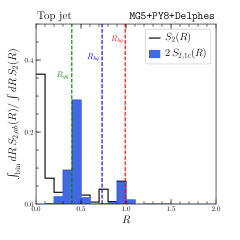
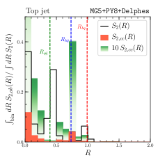
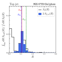
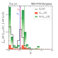
The information of the three-prong substructure is more clearly encoded in $S_{2,11}$, $S_{2,1c}$, and $S_{2,cc}$. The two-point correlations of the top jets corresponding to figure 2(a) and figure 2(b) are shown in figure 4 and figure 5, respectively. This decomposition of a given jet into $\mathbf{J}_{1}$ and $\mathbf{J}\setminus\mathbf{J}_{1}$ factorizes the identification of a three-prong structure into that of two-prong substructures and its relative position from the $\mathbf{J}_{1}$. Those $S_{2,ab}$ in parton level are as follows,

$$S_{2,11}(R) = p_{T,i_{1}}^{2}\delta(R),$$ (17)

$$2\,S_{2,1c}(R) = 2p_{T,i_{1}}p_{T,i_{2}}\delta(R-R_{i_{1}i_{2}})+2p_{T,i_{1}}p_{T,i_{3}}\delta(R-R_{i_{1}i_{3}}),$$ (18)

$$S_{2,cc}(R) = (p_{T,i_{2}}^{2}+p_{T,i_{3}}^{2})\delta(R)+2p_{T,i_{2}}p_{T,i_{3}}\delta(R-R_{i_{2}i_{3}}),$$ (19)

where $i_{k}$ is the $k$-th leading $p_{T}$ parton. Figure 4 shows that the two peaks are in $S_{2,1c}$ and the other two peaks are in $S_{2,cc}$. Figure 5 is the case where values of $R_{bq}$ and $R_{b\bar{q}}$ are similar. The $S_{2,cc}$ distribution has a peak at $R\approx 0.6$, and the peak intensity is comparable to that of the peak at $R=0$ because the $\mathbf{J}\setminus\mathbf{J}_{1}$ has a two-prong substructure. In addition, the $S_{2,1c}$ distribution suggests that the high $p_{T}$ constituents of $\mathbf{J}\setminus\mathbf{J}_{1}$ are away from $\mathbf{J}_{1}$ by a distance of $0.5$. Note that the analysis on $S_{2,1c}$ is essentially telescoping jets Chien:2013kca ; Chien:2017xrb with respect to $\mathbf{J}_{1}$.

Figure 4: $S_{2,1c}$ and $S_{2,cc}$ distributions of the top jet in figure 2(a). The intensity of $S_{2,cc}$ is much smaller than $S_{2}$ because the subleading $p_{T}$ jets have small transverse momenta. The magnified distribution of $S_{2,cc}$ is shown in the green histogram. The dashed lines are the characteristic angular scales at the parton level.

Figure 5: Same as figure 4 but the top jet in figure 2(b).

3 Morphological Analysis of Soft Emissions

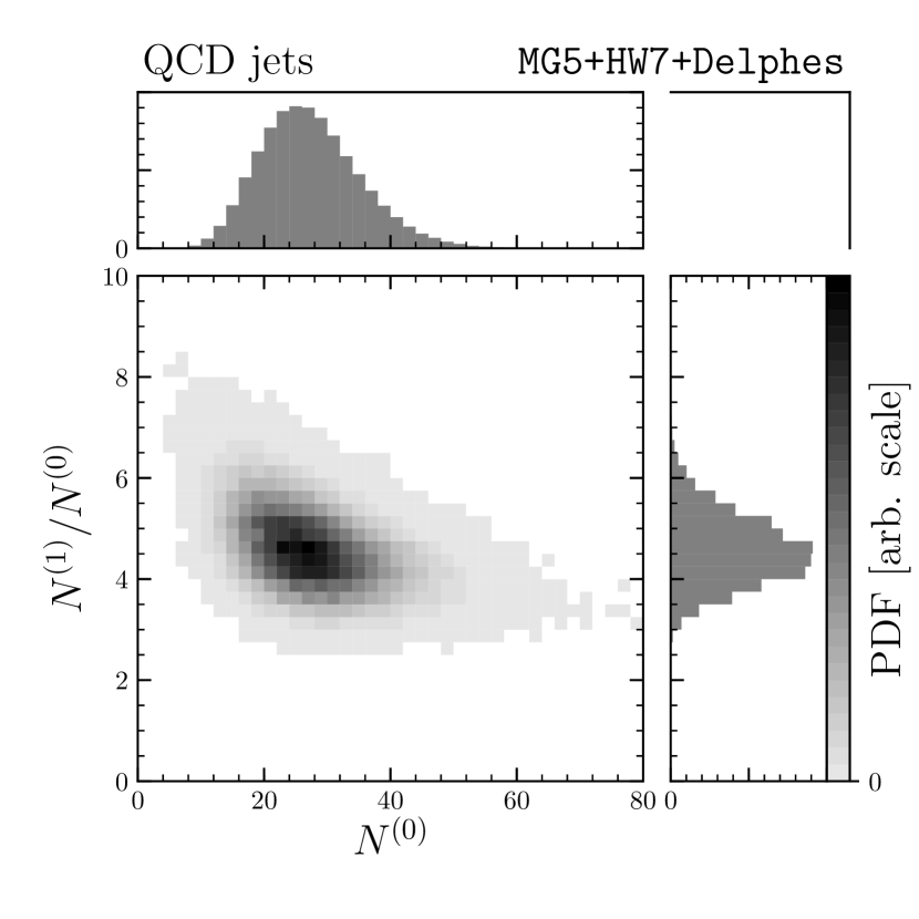
The number of particles of top jets and QCD jets is significantly different. For the boosted top quark decaying hadronically, i.e., $t\rightarrow bW\rightarrow bq\bar{q}^{\prime}$, the significant fraction of energy goes to color singlet $W$ boson. The number of particles in a top jet is less than that of a gluon jet with the same jet mass and momentum, and the particles are concentrated near the quark directions. The number of active pixels in the jet image, $N_{\mathrm{pixel}}$, is correlated to the number of particles in the jet, and therefore, it should be a crucial quantity of the jet image in the classification. This quantity is IRC unsafe as $E\rightarrow 0$ and depends on the physics at a low energy scale, and its accuracy of the theoretical prediction is limited. Indeed PY8 and HW7 predict significantly different pixel distributions for gluon jets, even though they are tuned to the experimental data.

To generalize the idea of $N_{\mathrm{pixel}}$, we introduce a morphological analysis of soft emissions on jet images. We consider two morphological operations: dilation, and filtering. Let $N^{(i)}$ be a number of pixels in a dilated image,

$$N^{(i)}=\#(\mathcal{V}^{(i)}),\quad i\in\{0,1,\cdots\},$$ (20)

where $\mathcal{V}^{(i)}$ is the Minkowski sum of the set of the $(\eta,\phi)$ coordinate vectors $\vec{R}_{i}$ of the active pixels, $\mathcal{V}^{(0)}$, and a set of discrete coordinate vectors on a square for dilation, i.e.,

$$\mathcal{V}^{(i)} = \mathcal{V}^{(0)}+\Delta R\times B^{(i)}=\{a+\Delta R\,b\ |\ a\in\mathcal{V}^{(0)},b\in B^{(i)}\},$$ (21)

$$B^{(i)} = \{(k,l)|k,l\in\{-i,-i+1,\cdots,i-1,i\}\}.$$ (22)

We denote a set of pixels whose centers belong to $\mathcal{V}^{(i)}$ as $\mathcal{P}^{(i)}$. Note that $\mathcal{P}^{(0)}$ is identical to the set of active pixels, and $N^{(0)}$ is $N_{\mathrm{pixel}}$. The set $\mathcal{P}^{(i)}$ is then a cover of the jet image, i.e., it is a union of the squares that attached to each active pixel. The covers obey a recurrence relation that $\mathcal{P}^{(i)}$ includes pixels in $\mathcal{P}^{(i-1)}$ and those touching one of the edges or corners of $\mathcal{P}^{(i-1)}$. This morphological mapping is illustrated in figure 6. Note that $N^{(i)}$ is proportional to the area $A^{(i)}$ of pixels in the cover $\mathcal{P}^{(i)}$ because each pixel has the same area $(\Delta R)^{2}$, i.e.,

$$A^{(i)}=(\Delta R)^{2}\times N^{(i)}.$$ (23)

For the analysis of soft activity, we consider a filtered image whose active pixels have $p_{T}$ larger than $E$. Let $N^{(i)}(E)$ be the number of active pixels in the filtered image. If we choose sufficiently large threshold $E$, the number $N^{(i)}(E)$ is relatively stable against the choice of the event simulators. The difference between the values of $N^{(i)}$ and $N^{(i)}(E)$ will provide us geometric information about the soft activity.

Figure 6: An illustration of the Minkowski sum in eq. (21). The most left figure shows the active pixels $\mathcal{P}^{(0)}$, the figure at the center shows the pixels whose centers are $B^{(1)}$, and $\mathcal{P}^{(1)}$ is shown in the right figure.

(a)

(b)

(c)

(d)

Figure 7: Illustrations of $\mathcal{P}^{(i)}$ for (a) an isolated pixel, (b) a line of pixels, (c) a $5\times 5$ square of pixels, (d) a ring of six pixels. For each plot, black pixels belongs to $P^{(0)}$; dark gray, light gray, blue pixels are the difference $P^{(i)}\setminus P^{(i-1)}$ for $i=1,2,3$, respectively.

The sequence of $N^{(i)}$ gives a quantitative description of the spatial distribution of pixels in the jet. Before going into some mathematical background, let us capture the idea using simple examples. Consider the relations between $N^{(0)}$ and $N^{(1)}$ of figure 7(a), figure 7(b), and figure 7(c):

1. Active pixels are separated by two or more pixels.

   $$N^{(1)}=9N^{(0)}$$ (24)

   This corresponds to the limit of sparse and scattered pixels.

2. Active pixels are aligned on a line.

   $$N^{(1)}=3N^{(0)}+6$$ (25)

   This case is the limit when soft activities come from a very narrow color string between two quarks at each end.

3. Active pixels are clustered in a square.

   $$N^{(1)}\sim(\sqrt{N^{(0)}}+2)^{2}$$ (26)

   This is the limit of a one-prong jet such as quark jet.

The ratio $N^{(1)}/N^{(0)}$ in large $N^{(0)}$ limit is approximately 9, 3, 1, respectively. If pixel clusters appear at small angular scale, $N^{(1)}/N^{(0)}$ is reduced. Therefore, $N^{(1)}/N^{(0)}$ quantifies the level of isolation of the pixels.

Figure 8: The Minkowski sum $\mathcal{P}^{(i)}$ of the top jet image and QCD jet image. For each plot, black pixels belongs to $P^{(0)}$ dark gray, light gray, blue pixels are the difference between $P^{(i)}-P^{(i-1)}$ for $i=1,2,3$, respectively.

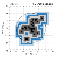
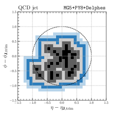
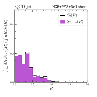
Figure 8 shows $\mathcal{P}^{(i)}$ of top and QCD jet images in figure 2(b) and figure 2(c), respectively. One quick observation is that $\mathcal{P}^{(i)}$ has some non-trivial structures for small $i$ ($i=0,1$), but the pixels quickly merge into a single cluster as the index $i$ increases. In the large angular scale ($i\geq 2$), the only relevant physics for the top jet vs. QCD jet classification is the color charge of the parent parton, and the $N^{(i)}$ does not carry significant additional information. In the next section, we show that $N^{(0)}$ and $N^{(1)}$ are sufficient to describe the soft structure contributing to the top jet and QCD jet classifier modeled by CNN.

The analysis based on the pixels can be generalized to the particle level analysis with a continuous parameter $R$ as follows. Let $\mathcal{P}(R)$ be a cover of particles on $(\eta,\phi)$ plane.

$$\mathcal{P}(R)=\bigcup_{i\in\mathbf{J}}B_{i}(R),$$ (27)

where $B_{i}(R)$ is a disk with radius $R$ and whose center is the direction vector $\vec{R}_{i}$ of a particle $i$. The area $A(R)$ of the cover $\mathcal{P}(R)$ is a quantity related to $N^{(i)}$, i.e., $A^{(i)}$ can be considered as a discrete analog of $A(R)$.

The change of $A(R)$ with respect to $R$ also quantifies the spacial distribution of particles. As far as all the disks are isolated, $A(R)/(\pi R^{2})$ is the number of particles. The ratio $A(R)/R^{2}$ decreases at the scale where the disks start overlapping. Therefore, the profile of $A(R)/R^{2}$ along $R$ encodes all the distances between particles.

A more general description of these morphological measures can be obtained from the integral geometry. According to Hadwiger’s theorem hadwigeb1956integralsatze , any geometric measure that has a notion of the size of a polyconvex set in Euclidean space $\mathbb{R}^{d}$ can be described by a set of functions called “Minkowski functionals.” The polyconvex set is a finite union of closed and bounded convex bodies. More precisely, the geometric measure $v$ should satisfy the following properties,

• Valuation: $v$ has a notion of size of a set. The value of $v$ of the empty set $\phi$ is zero, i.e, $v(\phi)=0$, and $v$ satisfies the following inclusion-exclusion property,

  $$v(B_{1}\cup B_{2})=v(B_{1})+v(B_{2})-v(B_{1}\cap B_{2})$$ (28)

  where $B_{1}$ and $B_{2}$ are polyconvex sets.

• Invariance: $v$ is invariant under any rotation and translation.

• Continuity: For any sequence of polyconvex sets $B_{n}$ that converges to $B$, its valuation $v(B_{n})$ also converges to $v(B)$.

Such geometric measures can be represented as a linear combination of $d+1$ Minkowski functionals $M_{i}$,

$$v(B)=\sum_{i=0}^{d}c_{i}M_{i}(B).$$ (29)

In $d=2$, we have three Minkowski functionals: area, perimeter, and Euler characteristic. Since $\mathcal{P}(R)$ on $(\eta,\phi)$ plane is a finite union of closed and bounded convex bodies $B_{i}(R)$, its geometry can be described by the Minkowski functionals. We already discussed the area $A(R)$ of $\mathcal{P}(R)$, and its perimeter $L(R)$ and Euler characteristic $\chi(R)$ are also useful quantities. The discrete analog of $L(R)$ and $\chi(R)$ can be used for analyzing jet images.

The Minkowski functionals show that $N^{(1)}$ carries independent information to $N^{(0)}$. We denote the perimeter and Euler characteristic of $\mathcal{P}^{(i)}$ as $L^{(i)}$ and $\chi^{(i)}$. If all the active pixels of a jet image are isolated enough, we may represent $A^{(1)}$ as $A^{(0)}+L^{(0)}\cdot(\Delta R)+4\chi^{(0)}\cdot(\Delta R)^{2}$ since $A^{(1)}$ is a valuation of $\mathcal{P}^{(0)}$. The relation between $N^{(0)}$ and $N^{(1)}$ is then as follows,

$$N^{(1)}=N^{(0)}+L^{(0)}/(\Delta R)+4\chi^{(0)}.$$ (30)

Note that this relation only holds when the squares attached to active pixels do not overlap each other. Once some squares start to overlap, the relation begins to deviate, and the persistence of this relation can be used as a morphological indicator for the topological change of $\mathcal{P}^{(i)}$. Therefore, $N^{(0)}$ and $N^{(1)}$ are effective variables for analyzing the geometry of soft particles of the jet image.

Figure 7(d) is an example that the sequence of $\mathcal{P}^{(i)}$ shows a non-trivial topological change. The sequence starts with six isolated pixels, $\mathcal{P}^{(1)}$ and $\mathcal{P}^{(2)}$ are a ring, and $\mathcal{P}^{(3)}$ is a single large cluster. The Euler characteristic $\chi^{(i)}$ and the perimeter $L^{(i)}$ of $\mathcal{P}^{(i)}$ are as follows.

$$\chi^{(i)} = (6,\ 0,\ 0,\ 1,\cdots)$$ (31)

$$\frac{L^{(i)}}{\Delta R} = (24,\ 52,\ 52,\ 54,\cdots).$$ (32)

The non-monotonic behavior of the sequence of Minkowski functionals for analyzing the topology of point distributions is often discussed in other literature Mecke:1994ax ; Schmalzing:1995qn . Utilizing this topological information for jet classification problems or global event topology analysis might be interesting, but the full analysis of the sequence of the Minkowski functionals is outside the scope of this paper.

Morphological analysis have been applied in physics to quantify the distribution of the objects. In Mecke:1994ax ; Schmalzing:1995qn , Minkowski functionals are used to identify the structure of the astrophysical objects. In more recent papers, persistence topology turns out to be useful tool for charcterizing seemingly random distribution of the points and applied in analysis of cosmic microwave background Cole:2017kve and string landscape Cole:2018emh . It is tempting to consider other roles of morphological analysis with Minkowski functionals in jet classifications.

4 Top Tagger based on Relation Network and Jet Morphology

In this section, we describe our setup of classifiers trained on the inputs discussed in the previous sections, $S_{2,ab}$ and $N^{(i)}$. These inputs are derivable from jet images, so the CNN performs better than those RNs in principle. We show that the deep learning on the small number of derived inputs reproduces the performance of the CNN. Therefore, those inputs are associated with the relevant physics for solving the classification problem. Moreover, the network using the derived inputs typically has less overfitting than that using the raw inputs.

4.1 Training Data and Model Implementation

We simulate top jet and QCD jet samples by Madgraph5 Alwall:2014hca , followed by Pythia 8 (PY8) Sjostrand:2014zea or Herwig 7 (HW7) Bellm:2015jjp ; Bahr:2008pv . The detector response of generated events is simulated by Delphes deFavereau:2013fsa . Jets are reconstructed by the anti-$k_{T}$ algorithm with radius parameter $R_{\mathbf{J}}=1.0$. The jet constituents are calorimeter towers with angular resolution approximately $\Delta R=0.1$. The details of the sample preparation are explained in appendix A.

We categorize the inputs to the RNs into the four sets: $\bm{x}_{\mathrm{trim}}$, $\bm{x}_{\mathbf{J}_{1}}$, $\bm{x}_{\mathrm{kin}}$, and $\bm{x}_{\mathrm{geometry}}$.

• $\bm{x}_{\mathrm{trim}}$ is a set of discretized $S_{2,\mathrm{trim}}$ and $S_{2,\mathrm{soft}}$ up to angular scale $R=1.5$,

  $$\bm{x}_{\mathrm{trim}} = (S_{2,\mathrm{trim}}^{(i)}|i=0,\cdots,14)\oplus(S_{2,\mathrm{soft}}^{(i)}|i=0,\cdots,14),$$ (33)

  where $S_{2,ab}^{(i)}$ is the binned spectrum of $S_{2,ab}$, with bin size $\Delta R$ in order to keep the same angular resolution to the jet image,

  $$S_{2,ab}^{(i)}=\frac{1}{\Delta R}\int_{i\Delta R}^{(i+1)\Delta R}dR\,S_{2,ab}(R)=\frac{1}{\Delta R}\sum_{\begin{subarray}{c}j\in\mathbf{J}_{a},k\in\mathbf{J}_{b}\\ R_{jk}\in[i\Delta R,(i+1)\Delta R)\end{subarray}}p_{T,j}p_{T,k}.$$ (34)

  We may consider the angular scale up to the diameter $2R_{\mathbf{J}}=2.0$, but $S_{2,\mathrm{trim}}^{(i)}$ and $S_{2,\mathrm{soft}}^{(i)}$ at such large $R$ are less useful Chakraborty:2019imr .

• $\bm{x}_{\mathbf{J}_{1}}$ is a set of discretized $S_{2,11}$, $S_{2,1c}$ and $S_{2,cc}$ as follows,

  $$\bm{x}_{\mathbf{J}_{1}} = (S_{2,11}^{(i)}|i=0,\cdots,3)\oplus(S_{2,1c}^{(i)}|i=0,\cdots,9)\oplus(S_{2,cc}^{i}|i=0,\cdots,14).$$ (35)

  Again, we consider spectra only up to the relevant angular scales. For $S_{2,11}^{(i)}$ and $S_{2,cc}^{(i)}$, the scale is the diameter of the corresponding subjet but too large angular scale is ignored. For $S_{2,1c}^{(i)}$, the scale is the jet radius because it is the correlation between the core part $\mathbf{J}_{1}$ and its surroundings.

• $\bm{x}_{\mathrm{kin}}$ is a set of global inputs,

  $$\bm{x}_{\mathrm{kin}}=(p_{T,\mathbf{J}},m_{\mathbf{J}},p_{T,\mathbf{J}_{\mathrm{trim}}},m_{\mathbf{J}_{\mathrm{trim}}},p_{T,\mathbf{J}\setminus\mathbf{J}_{1}},m_{\mathbf{J}\setminus\mathbf{J}_{1}}).$$ (36)

  In addition to the transverse momenta, we include the masses as the inputs because $2m_{\mathbf{J}_{a}}/p_{T,\mathbf{J}_{a}}$ is a characteristic angular scale of $\mathbf{J}_{a}$.

• $\bm{x}_{\mathrm{geometry}}$ is a set of the numbers of pixels of the jet images $\mathcal{P}^{(0)}$ and $\mathcal{P}^{(1)}$,

  $$\bm{x}_{\mathrm{geometry}} = (N^{(0)},N^{(1)},N^{(0)}(4\,\mathrm{GeV}),N^{(1)}(4\,\mathrm{GeV})).$$ (37)

We modularize the implementations of the model outputs $\bm{u}^{\prime}=\phi^{u}(\bm{x})$ to avoid the curse of dimensionality. When inputs are too many, there is a potential danger of overfitting due to sparsely distributed samples. In our previous work, we use $\sim 40$ inputs for the classification of Higgs jets and QCD jets Lim:2018toa ; Chakraborty:2019imr . The inputs for the classification of top jets and QCD jets are increased to $\sim 70$, and training of a simple MLP classifier on these inputs may have difficulties. Therefore, we compress $\bm{x}_{\mathrm{trim}}$ and $\bm{x}_{\mathbf{J}_{1}}$ to a smaller number of hidden variables $\bm{h}_{\mathrm{trim}}$ and $\bm{h}_{\mathbf{J}_{1}}$ by a neural network and get $\bm{u}^{\prime}$ from them. The following is the closed-form expression of $\mathrm{RN}_{S_{2}}$ that uses only the IRC safe inputs: $\bm{x}_{\mathrm{trim}}$, $\bm{x}_{\mathbf{J}_{1}}$, and $\bm{x}_{\mathrm{kin}}$.

$$\bm{h}_{\mathrm{trim}} = \mathrm{MLP}_{\mathrm{trim}}(\bm{x}_{\mathrm{trim}},\bm{x}_{\mathrm{kin}};\bm{\theta}_{\mathrm{trim}}),$$ (38)

$$\bm{h}_{\mathbf{J}_{1}} = \mathrm{MLP}_{\mathbf{J}_{1}}(\bm{x}_{\mathbf{J}_{1}},\bm{x}_{\mathrm{kin}};\bm{\theta}_{\mathbf{J}_{1}}),$$ (39)

$$\bm{u}^{\prime} = \mathrm{MLP}_{\mathrm{logit}}(\bm{h}_{\mathrm{trim}},\bm{h}_{\mathbf{J}_{1}},\bm{x}_{\mathrm{kin}};\bm{\theta}_{\mathrm{logit}}),$$ (40)

where $\mathrm{MLP}_{a}$ is a multilayer perceptron (MLP) and $\bm{\theta}_{a}$ are its trainable parameters. We provide $\bm{x}_{\mathrm{kin}}$ to each network to tell the characteristic angular scales directly. We use the exponential linear unit (ELU) DBLP:journals/corr/ClevertUH15 as the activation function of each MLP. The dimensions of $\bm{h}_{\mathrm{trim}}$ and $\bm{h}_{\mathbf{J}_{1}}$ are 5. The output $\bm{u}^{\prime}$ is a dimension two vector and will be transformed into the softmax outputs for the binary classification purpose.

$$\hat{y}^{i}=\frac{\mathrm{exp}(u^{\prime}_{i})}{\mathrm{exp}(u^{\prime}_{0})+\mathrm{exp}(u^{\prime}_{1})},\quad i=0,1$$ (41)

When the geometric information $\bm{x}_{\mathrm{geometry}}$ is included in the inputs, we use them as arguments of $\mathrm{MLP}_{\mathrm{logit}}$,

$$\bm{u}^{\prime} = \mathrm{MLP}_{\mathrm{logit}}(\bm{h}_{\mathrm{trim}},\bm{h}_{\mathbf{J}_{1}},\bm{x}_{\mathrm{kin}},\bm{x}_{\mathrm{geometry}};\bm{\theta}_{\mathrm{logit}})$$ (42)

We consider three additional relation networks that uses the geometric information: $\mathrm{RN}_{S_{2},N^{(0)}}$, $\mathrm{RN}_{S_{2},N^{(0)},N^{(0)}(4\,\mathrm{GeV})}$, and $\mathrm{RN}_{S_{2},N^{(0)},N^{(1)}}$. Their inputs are listed in table 1. The detailed implementations of these RNs are in appendix C.1.

model	$\bm{x}_{\mathrm{kin}}$	$\bm{x}_{\mathrm{trim}}$	$\bm{x}_{\mathbf{J}_{1}}$	$\bm{x}_{\mathrm{geometry}}$
				$N^{(0)}$	$N^{(0)}(4\,\mathrm{GeV})$	$N^{(1)}$	$N^{(1)}(4\,\mathrm{GeV})$
$\mathrm{RN}_{S_{2}}$	$\bigcirc$	$\bigcirc$	$\bigcirc$
$\mathrm{RN}_{S_{2},N^{(0)}}$	$\bigcirc$	$\bigcirc$	$\bigcirc$	$\bigcirc$
$\mathrm{RN}_{S_{2},N^{(0)},N^{(0)}(4\,\mathrm{GeV})}$	$\bigcirc$	$\bigcirc$	$\bigcirc$	$\bigcirc$	$\bigcirc$
$\mathrm{RN}_{S_{2},N^{(0)},N^{(1)}}$	$\bigcirc$	$\bigcirc$	$\bigcirc$	$\bigcirc$	$\bigcirc$	$\bigcirc$	$\bigcirc$

Table 1: The list of inputs used in each RN. The circle represents that the given input is used. The CNN trained on jet images can utilize all this information.

The softmax output is trained by minimizing the cross-entropy loss function. In addition, we marginalize the $p_{T,\mathbf{J}}$ distribution in the classification because the top jet samples and QCD jet samples have different $p_{T,\mathbf{J}}$ distributions. To do this, we train networks in a way that interpolates binary classifiers for the jets at given $p_{T,\mathbf{J}}$. The corresponding cross-entropy loss function $\mathcal{L}_{\mathrm{CE}}$ is as follows.

$$\mathrm{CE}(p_{T,\mathbf{J}};\bm{\theta}) = -\frac{1}{2}\sum_{Y=\mathrm{top,QCD}}\int d\tilde{\bm{x}}f_{\tilde{\bm{x}}|p_{T,\mathbf{J}}}(\tilde{\bm{x}};Y)\,\sum_{i=0,1}y_{Y}^{i}\log\hat{y}^{i}(\bm{x};\bm{\theta})$$ (43)

$$\mathcal{L}_{\mathrm{CE}}(\bm{\theta}) = \frac{1}{p_{T,\mathbf{J}}^{\max}-p_{T,\mathbf{J}}^{\min}}\int_{p_{T,\mathbf{J}}^{\min}}^{p_{T,\mathbf{J}}^{\max}}dp_{T,\mathbf{J}}\,\mathrm{CE}(p_{T,\mathbf{J}};\bm{\theta})$$ (44)

where $Y$ is a category label, $y_{\mathrm{top}}=(1,0)$, and $y_{\mathrm{QCD}}=(0,1)$. The function $f_{\tilde{\bm{x}}|p_{T,\mathbf{J}}}(\bm{\tilde{x}};Y)$ is the conditional probability density of $\tilde{\bm{x}}$ given $p_{T,\mathbf{J}}$, and $\tilde{\bm{x}}$ is $\bm{x}$ without $p_{T,\mathbf{J}}$.

The integral can be approximated by a Monte-Carlo integration,

$$\mathcal{L}_{\mathrm{CE}}(\bm{\theta}) \approx -\frac{1}{2}\sum_{Y=\mathrm{top,QCD}}\sum_{i_{Y}=1}^{N_{Y}}\frac{1}{f_{p_{T,\mathbf{J}}}(p_{T,\mathbf{J}}^{[i_{Y}]};Y)}\,\sum_{i=0,1}y_{Y}^{i}\log\hat{y}^{i}(\bm{x}^{[i_{Y}]};\bm{\theta})$$ (45)

where $f_{p_{T,\mathbf{J}}}(p_{T,\mathbf{J}};Y)$ is the probability density function of $p_{T,\mathbf{J}}$ given $Y$, and the variables with superscript $[i_{Y}]$ is the value at the $i_{Y}$-th sample in the training dataset of $Y$. The probability density function $f_{p_{T,\mathbf{J}}}(p_{T,\mathbf{J}};Y)$ is modeled by kernel density estimation (KDE) described in appendix B. The resulting loss function is essentially a cross-entropy with samples whose $p_{T,\mathbf{J}}$ distribution is reweighted to be uniform. In addition to this cross-entropy loss, $L_{2}$ regularizer $\mathcal{L}_{\mathrm{reg}}$ NIPS1988_156 ; NIPS1990_323 ; NIPS1991_563 with the weight decay constant $\lambda=0.001$ is added to regularize $\mathrm{MLP}_{a}$.

$$\mathcal{L}_{\mathrm{reg}}=\frac{\lambda}{2}\sum_{a}|\bm{W}_{a}|^{2}$$ (46)

where $\bm{W}_{a}$ are the weights of hidden layers in $\mathrm{MLP}_{a}$.

The training setup is as follows. We minimize the loss function $\mathcal{L}(\bm{\theta})=\mathcal{L}_{\mathrm{CE}}(\bm{\theta})+\mathcal{L}_{\mathrm{reg}}(\bm{\theta})$ by ADAM optimizer ADAM with learning rate 0.001, the first moment exponential moving average coefficient $\beta_{1}=0.9$, the second moment exponential moving average coefficient $\beta_{2}=0.999$, and stabilization constant $\epsilon=10^{-7}$. Batched samples are used in order to reduce overfitting. The weights of the MLP are initialized by the He initializer He_2015_ICCV , and the biases are initialized to be zero. We will use early stopping for the termination criterion, but there is a chance that the network is mildly overfitted to the validation dataset during learning the features of the rare events. If the gradients from the rare events distort the trained results for the dominant events, the network parameters have to be corrected again, and the training becomes noisy. The random overfitting to the validation sample occurs during this noisy learning on the rare events. To avoid this artifact, we use the exponential moving averages $\hat{\bm{\theta}}^{(t)}$ of the trainable parameters $\bm{\theta}^{(t)}$ at the epoch $t$ for the validation and testing. The details of the moving average can be found in appendix D. We monitor the loss $\mathcal{L}_{\mathrm{tot}}(\hat{\bm{\theta}})$ of the validation samples during the training and terminate the training if the loss function does not improve during 50 latter epochs. The networks and training setup is implemented in Keras chollet2015keras with TensorFlow tensorflow2015-whitepaper backend. Optimization on the batch number is performed by the grid search. We iterate the training for batch numbers, 20, 50, and 100 and two different random number seeds.

The results of the RN-based classifier will be compared to that of a CNN-based classifier. The CNN model is similar to that of the previous paper Chakraborty:2019imr but with more nodes and layers. The closed-form expression of the CNN is as follows,

$$\bm{h}_{\mathrm{image}} = \mathrm{CNN}_{\mathrm{image}}(\bm{x}_{\mathrm{image}};\bm{\theta}_{\mathrm{CNN}})$$ (47)

$$\bm{u}^{\prime} = \mathrm{MLP}_{\mathrm{logit}}(\bm{h}_{\mathrm{image}},\bm{x}_{\mathrm{kin}};\bm{\theta}_{\mathrm{MLP}}),$$ (48)

where $\bm{x}_{\mathrm{image}}$ is energy deposits of the preprocessed jet image described in appendix C.2. The module $\mathrm{CNN}_{\mathrm{image}}$ consists of 6 two-dimensional convolutional layers with $3\times 3$ filters and ELU activations. We insert two $2\times 2$ max-pooling layers after the third and sixth convolutional layers. The $\bm{h}_{\mathrm{image}}$ are the flattened outputs of the $\mathrm{CNN}_{\mathrm{image}}$. The model outputs $\bm{u}^{\prime}$ are from an MLP analyzing $\bm{h}_{\mathrm{image}}$ together with the kinematic information $\bm{x}_{\mathrm{kin}}$. The detailed implementation of this CNN is in appendix C.2. The training setup is the same as that of the RNs, but we check batch numbers 100, 200, and 500 instead because of the limitation of GPU memory.

4.2 Classification results

Figure 9: The ROC curves of the networks trained on PY8 samples.

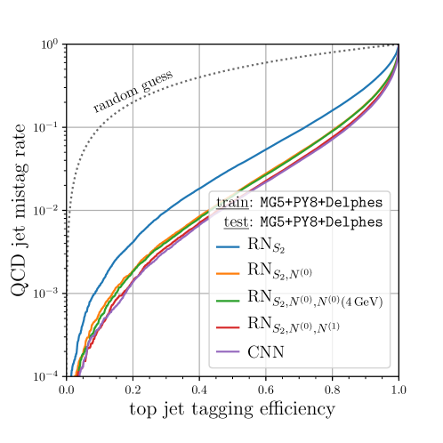
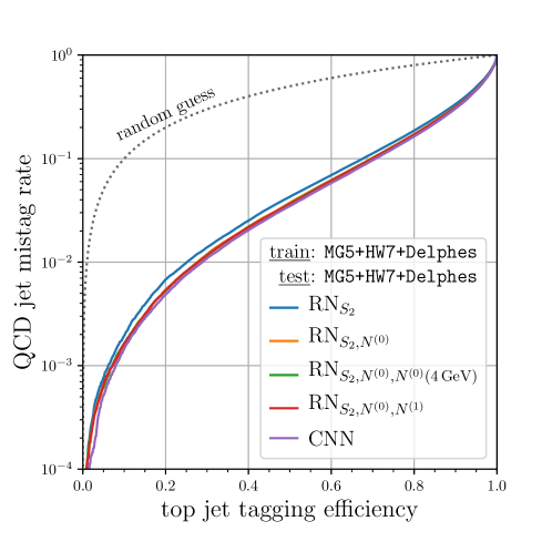
Figure 9 shows the ROC curves of the networks trained on PY8 samples. The AUC, which is the upper area of each curve, of $\mathrm{RN}_{S_{2}}$, $\mathrm{RN}_{S_{2},N^{(0)}}$, $\mathrm{RN}_{S_{2},N^{(0)},N^{(1)}}$, and $\mathrm{CNN}$ are 0.8990, 0.9352, 0.9442, and 0.9465, respectively. There is a large gap between the ROC curves of $\mathrm{RN}_{S_{2}}$ and $\mathrm{CNN}$. This gap is partially filled by including an additional input $N^{(0)}$, as shown in the ROC curve of $\mathrm{RN}_{S_{2},N^{(0)}}$. Surprisingly, when we consider all the geometric inputs $\bm{x}_{\mathrm{geometry}}$, the ROC curve of $\mathrm{RN}_{S_{2},N^{(0)},N^{(1)}}$ is almost equal to that of the CNN. Therefore, the inputs $\bm{x}_{\mathrm{trim}}$, $\bm{x}_{\mathbf{J}_{1}}$, $\bm{x}_{\mathrm{kin}}$, and $\bm{x}_{\mathrm{geometry}}$ can be considered as useful middle-level variables for modeling the top jet classifier.

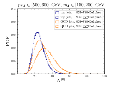
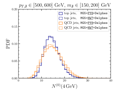
The reason for a big gap between the ROC curves of $\mathrm{RN}_{S_{2}}$ and $\mathrm{CNN}$ is the difference in $N^{(0)}$ distributions between top jet samples and QCD jet samples. The QCD jets in this paper are leading $p_{T}$ jets of $pp\rightarrow jj$ so that they are mostly gluon jets, which have a large $N^{(0)}$ than a jet from a color triplet parton. In addition, PY8 predicts significantly higher $N^{(0)}$ of gluon jets than HW7, as in figure 10. Similar situations have been pointed out for the counting variables such as the charged track multiplicity Gallicchio:2012ez , and the soft drop multiplicity Frye:2017yrw .

Figure 10: $N^{(0)}$ and $N^{(0)}(4\,\mathrm{GeV})$ distributions of PY8 and HW7 data sets. The blue histograms are for the top jets, and the orange histograms are for QCD jets. The solid lines are for PY8 generated samples, and the dashed lines are for HW7 generated samples.

The situation may be compared with the classification of Higgs jets and QCD jets, studied in Lim:2018toa . In this case, the difference between the ROC curves of $\mathrm{RN}_{S_{2}}$ and $\mathrm{CNN}$ is tiny. QCD jet samples in the study are leading $p_{T}$ jets of $pp\rightarrow Zj$ with invisibly decaying $Z$ boson, and most of the samples are the quark jets. The difference in the $N^{(0)}$ distribution of the Higgs jets and QCD jets is small, and therefore, $N^{(0)}$ does not play an important role there.

The remaining gap between the ROC curves of $\mathrm{RN}_{S_{2},N^{(0)}}$ and $\mathrm{CNN}$ is almost filled by including $N^{(1)}$ in the analysis. As discussed in the previous section, the ratio $N^{(1)}/N^{(0)}$ is a morphological measure that quantifies the level of clustering of the pixels. Therefore, $N^{(1)}$ is useful for distinguishing compact top jets from QCD jets whose number of pixels is the same. The similarity of two ROC curves indicates that the information summarized in the Minkowski functionals is used in the jet image analysis.

Not only $\mathrm{RN}_{S_{2},N^{(0)},N^{(1)}}$ gives a comparable result to $\mathrm{CNN}$, but it is also significantly more stable. We compare the softmax output $\hat{y}^{0}$ of a network $\mathcal{N}$ and the output of the same network trained with a different random seed, and we call the alternative output $\hat{y}^{\prime\,0}$. The change of the seed affects the shuffling of the events between batches and alters the initialization of the network. Since the training of the neural network is not a convex optimization in general, the network output difference $\Delta\hat{y}^{0}[\mathcal{N}]=\hat{y}^{\prime\,0}[\mathcal{N}]-\hat{y}^{0}[\mathcal{N}]\neq 0$. In figure 11, we show the histogram of two outputs $(\hat{y}^{0},\hat{y}^{\prime\,0})$ for $\mathrm{RN}_{S_{2},N^{(0)},N^{(1)}}$ and $\mathrm{CNN}$. The distribution for $\mathrm{RN}_{S_{2},N^{(0)},N^{(1)}}$ is narrower than that for $\mathrm{CNN}$. This shows that training of $\mathrm{RN}_{S_{2},N^{(0)},N^{(1)}}$ is more stable.

The better training stability of $\mathrm{RN}$ is due to the difference in the inputs of the functional model. The pair of preprocessed jet image and $\bm{x}_{\mathrm{kin}}$ contain more information than the two-point energy correlations and Minkowski functionals. Hence, $\mathrm{CNN}$ could approximate a wider variety of functions of jet constituents than $\mathrm{RN}$. In other words, the training of CNN requires more effort in order to scan over larger space of functions. The training of a simpler model is much stable than that of a complex model because of less number of inputs and trainable parameters. A simpler model has a potential danger of underfitting, but it is less severe in $\mathrm{RN}$ because $S_{2,ab}$ and $N^{(i)}$ are reasonable set for describing functional space of energy correlation and geometry of the jet constituents, respectively.

Figure 11: The distribution of softmax output of the classifiers for different random seed. upper two figures for $\hat{y}^{0}[\mathrm{RN}_{S_{2},N^{(0)},N^{(1)}}]$, and the bottom two figures for $\hat{y}^{0}[\mathrm{RN}_{S_{2},N^{(0)},N^{(1)}}]$. The left figures are top jets and the right figures are QCD jets.

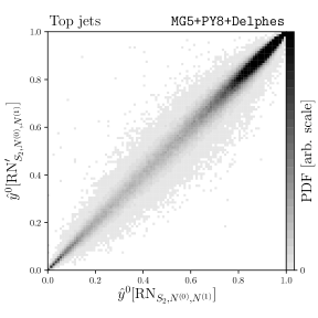
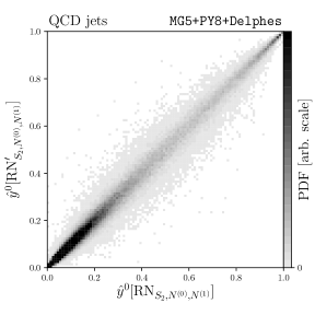
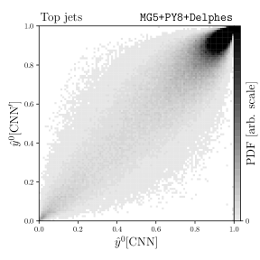
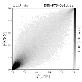
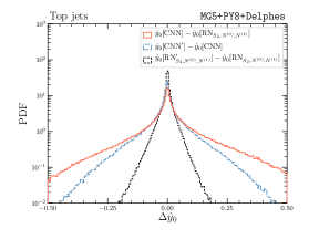
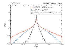
We now compare the outputs $\hat{y}^{0}[\mathrm{CNN}]$ and $\hat{y}^{0}[\mathrm{RN}]=\hat{y}^{0}[\mathrm{RN}_{S_{2},N^{(0)},N^{(1)}}]$. Figure 12 shows the distributions of $\Delta\hat{y}^{0}[\mathrm{RN}]$, $\Delta\hat{y}^{0}[\mathrm{CNN}]$, and $\Delta\hat{y}^{0}[\mathrm{CNN},\mathrm{RN}]=\hat{y}^{0}[\mathrm{CNN}]-\hat{y}^{0}[\mathrm{RN}]$. The mean and standard deviation of these differences are summarized in table 2. All the $\Delta\hat{y}^{0}$ distributions are sharply peaked approximately at $\Delta\hat{y}^{0}=0$, which indicates that the classifiers make the same decision for the majority of the events. Since the training of the $\mathrm{CNN}$ is less stable than that of $\mathrm{RN}$, the standard deviation $\sigma(\Delta\hat{y}^{0}[\mathrm{CNN}])$ of $\Delta\hat{y}^{0}[\mathrm{CNN}]$ is much larger than $\sigma(\Delta\hat{y}^{0}[\mathrm{RN}])$ of $\Delta\hat{y}^{0}[\mathrm{RN}]$. The standard deviation of $\Delta\hat{y}^{0}[\mathrm{CNN},\mathrm{RN}]$ is larger than the error $\sqrt{\sigma(\Delta\hat{y}^{0}(\mathrm{CNN}))^{2}+\sigma(\Delta\hat{y}(\mathrm{RN}))^{2}}$, which is 0.091 for the top jet samples and 0.095 for the QCD jet samples. This indicates that the outputs of $\mathrm{RN}$ and $\mathrm{CNN}$ are highly correlated, but there are still some differences. We repeat the same analysis on non-typical events, which satisfies $0.15<\hat{y}^{0}<0.85$ for one of $\mathrm{RN}$ or $\mathrm{CNN}$. The results are similar, but the standard deviations are larger by a factor 1.5 because we removed samples easy to classify.

output difference	top jet samples		QCD jet samples
	average	deviation	average	deviation
$\Delta\hat{y}^{0}[\mathrm{RN}]$$\Delta\hat{y}^{0}[\mathrm{CNN},\mathrm{RN}]$ $=\hat{y}^{\prime 0}[\mathrm{RN}]-\hat{y}^{0}[\mathrm{RN}]$	$-9.56\times 10^{-4}$	0.0271	$-1.65\times 10^{-4}$	0.0279
$\Delta\hat{y}^{0}[\mathrm{CNN}]$$\Delta\hat{y}^{0}[\mathrm{CNN},\mathrm{RN}]$ $=\hat{y}^{\prime 0}[\mathrm{CNN}]-\hat{y}^{0}[\mathrm{CNN}]$	$-1.46\times 10^{-3}$	0.0867	$-6.14\times 10^{-3}$	0.0911
$\Delta\hat{y}^{0}[\mathrm{CNN},\mathrm{RN}]$ $=\hat{y}^{0}[\mathrm{CNN}]-\hat{y}^{0}[\mathrm{RN}]$	$\phantom{-}6.98\times 10^{-3}$	0.1410	$\phantom{-}3.10\times 10^{-3}$	0.1440
$\Delta\hat{y}^{0}[\mathrm{CNN},\mathrm{RN}]=$ $\hat{y}^{\prime 0}[\mathrm{CNN}]-\hat{y}^{0}[\mathrm{RN}]$	$\phantom{-}5.51\times 10^{-3}$	0.1370	$\phantom{-}9.26\times 10^{-3}$	0.1420
after selection: $0.15<\hat{y}^{0}[\mathrm{RN}_{S_{2},N^{(0)},N^{(1)}}]<0.85$ or $0.15<\hat{y}^{0}[\mathrm{CNN}]<0.85$
$\Delta\hat{y}^{0}[\mathrm{RN}]$$\Delta\hat{y}^{0}[\mathrm{CNN},\mathrm{RN}]$ $=\hat{y}^{\prime 0}[\mathrm{RN}]-\hat{y}^{0}[\mathrm{RN}]$	$-1.60\times 10^{-3}$	0.0403	$-1.06\times 10^{-3}$	0.0409
$\Delta\hat{y}^{0}[\mathrm{CNN}]$$\Delta\hat{y}^{0}[\mathrm{CNN},\mathrm{RN}]$ $=\hat{y}^{\prime 0}[\mathrm{CNN}]-\hat{y}^{0}[\mathrm{CNN}]$	$\phantom{-}3.64\times 10^{-3}$	0.129	$\phantom{-}3.51\times 10^{-3}$	0.131
$\Delta\hat{y}^{0}[\mathrm{CNN},\mathrm{RN}]=\hat{y}^{0}[\mathrm{CNN}]-\hat{y}^{0}[\mathrm{RN}]$	$\phantom{-}1.61\times 10^{-2}$	0.215	$\phantom{-}3.50\times 10^{-3}$	0.217
$\Delta\hat{y}^{0}[\mathrm{CNN},\mathrm{RN}]=$ $\hat{y}^{\prime 0}[\mathrm{CNN}]-\hat{y}^{0}[\mathrm{RN}]$	$\phantom{-}1.97\times 10^{-2}$	0.206	$\phantom{-}9.39\times 10^{-3}$	0.210

Table 2: Average and standard deviation of the output difference $\Delta y^{0}$.

Figure 12: The difference of softmax output for various models, $\Delta\hat{y}^{0}[\mathrm{RN}]$, $\Delta\hat{y}^{0}[\mathrm{CNN}]$, and $\Delta\hat{y}^{0}[\mathrm{CNN},\mathrm{RN}]$ for top jets and QCD jets.

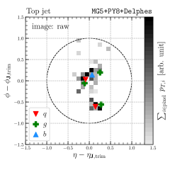
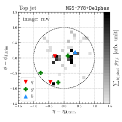
In order to understand the cases on which $\mathrm{RN}_{S_{2},N^{(0)},N^{(1)}}$ and $\mathrm{CNN}$ gives us extremely different answers, we show two examples in figure 13. To choose jets with stable $\mathrm{CNN}$ predictions, the selected jets have similar $\hat{y}^{0}[\mathrm{CNN}]$ and $\hat{y}^{\prime 0}[\mathrm{CNN}]$. For the left jet image, $\mathrm{CNN}$ judges the jet as a top jet while $\mathrm{RN}$ does not. The $b$ quark and one of the light quarks accidentally overlap in this event. This type of event is certainly not typical. The probability that the angle $R_{bq}$ or $R_{b\bar{q}}$ is less than 0.2 is 5.6% without considering spin-correlation. For the right jet image, $\mathrm{CNN}$ judges that the jet is a QCD jet, but $\mathrm{RN}$ does not. It is a two-prong jet with many soft radiations and a small $p_{T}$ subjet from a quark due to longitudinal decay of W boson. In the longitudinal decay, one of the quark goes backward to the boost direction, but these jets suppressed in the phase space. Because both of the top jets are not typical, it is not surprising the two different models give very different results for those events.

Figure 13: Jets images of top jets that $\mathrm{RN}_{S_{2},N^{(0)},N^{(1)}}$ and $\mathrm{CNN}$ give different answers. The network outputs of each jet image are as follows: (left) $\hat{y}^{0}[\mathrm{RN}_{S_{2},N^{(0)},N^{(1)}}]=0.0795$, $\hat{y}^{0}[\mathrm{CNN}]=0.908$, $\hat{y}^{\prime 0}[\mathrm{CNN}]=0.883$, (right) $\hat{y}^{0}[\mathrm{RN}_{S_{2},N^{(0)},N^{(1)}}]=0.836$, $\hat{y}^{0}[\mathrm{CNN}]=0.0905$, $\hat{y}^{\prime 0}[\mathrm{CNN}]=0.101$,

We have checked if more aggressive training on these rare events improves the performance, for example, relaxing the regularizer setup. The AUCs of $\mathrm{RN}$ and $\mathrm{CNN}$ with the weight decay constant $\lambda=10^{-4}$ are 0.9461 and 0.9465, respectively. There are tiny improvements in the classification performance, but it comes together with overfitting. The validation loss $\mathcal{L}(\hat{\bm{\theta}})$ and training loss $\mathcal{L}({\bm{\theta}})$ are 0.3044, and 0.2969 for $\mathrm{RN}$; 0.3201, and 0.2971 for $\mathrm{CNN}$, respectively. The $\mathcal{L}(\hat{\bm{\theta}})$ and $\mathcal{L}({\bm{\theta}})$ in the original setup are 0.3076, and 0.3049 for $\mathrm{RN}_{S_{2},N^{(0)},N^{(1)}}$; 0.3338, and 0.3371 for the $\mathrm{CNN}$. The difference between the training and validation loss is much bigger in $\lambda=10^{-4}$ setup, which is a sign of overfitting.

4.3 Alternative vertex label choice

Vertex label is a hyperparameter of the RNs, and we use labels based on the trimmed jet and leading $p_{T}$ subjet in order to explicitly identify hard substructures and subleading $p_{T}$ substructures. Other labels may be used depending on the purpose. For example, trimming may be replaced with recursive soft drop (RSD) Larkoski:2014wba ; Dreyer:2018tjj for better analytic tractability of the two-point energy correlations. Let $\mathbf{J}_{r}$ be the groomed jet by the RSD, and $r$ be its vertex label. We define $S_{2,\mathrm{RSD}}$ and $S_{2,\mathrm{RSD}^{c}}$,

$$S_{2,\mathrm{RSD}}(R) = S_{2,rr}(R),$$ (49)

$$S_{2,\mathrm{RSD}^{c}}(R) = S_{2}(R)-S_{2,rr}(R),$$ (50)

corresponding to $S_{2,\mathrm{trim}}$ and $S_{2,\mathrm{soft}}$, respectively. Figure 14 shows the $S_{2,\mathrm{RSD}}$ distribution of the top jets and QCD jet in figure 2, but the difference is small. The two-point energy correlation related to the soft activity that satisfies the soft drop condition may be included in $S_{2,\mathrm{RSD}}$.

(a)

(b)

(c)

Figure 14: The $S_{2}$ and $S_{2,\mathrm{RSD}}$ distributions of the top jets and the QCD jet in figure 2. The dashed lines are the characteristic angular scales of the top jets in the parton level.

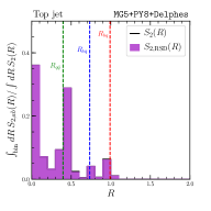
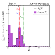
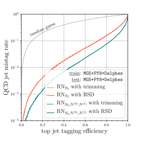
Figure 15 shows the ROC curves of $\mathrm{RN}_{S_{2}}$ and $\mathrm{RN}_{S_{2},N^{(0)},N^{(1)}}$ after replacing inputs $S_{2,\mathrm{trim}}$, $S_{2,\mathrm{soft}}$, $p_{T,\mathbf{J}_{h}}$, and $m_{\mathbf{J}_{h}}$ to $S_{2,\mathrm{RSD}}$, $S_{2,\mathrm{RSD}^{c}}$, $p_{T,\mathbf{J}_{r}}$, and $m_{\mathbf{J}_{r}}$, respectively. The performance does not change much because the change of inputs is simply a rearrangement of $S_{2}$ bins related to the soft activity that satisfies the soft drop condition. Therefore, the impact on the top jet classification performance due to the change of groomer is small.

Figure 15: The ROC curves of $\mathrm{RN}_{S_{2}}$ and $\mathrm{RN}_{S_{2},N^{(0)},N^{(1)}}$ with trimming or RSD.

4.4 Discussion on other top taggers

So far, we compare the performance of the RNs to that of the CNN. In this subsection, we comment on other top taggers.

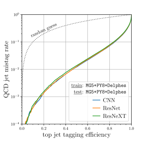
In Kasieczka:2019dbj , ParticleNet Qu:2019gqs ; 10.1145/3326362 and ResNeXt Xie_2017_CVPR show a better performance in the top jet classification than the CNN. One may wonder if additional features should be included in the RN inputs to reproduce their performance. However, the networks on figure 5 of Kasieczka:2019dbj are not trained on inputs at the same angular resolution. It is not clear if the better networks learn additional physical features. The ResNeXt and CNN in Kasieczka:2019dbj use jet images with pixel size 0.025 and 0.04, respectively. We especially find that the performances of ResNeXt and CNN trained on jet images with pixel size 0.1 are similar. Figure 16 shows their ROC curves.

The ResNet 7780459 and ResNeXt in Figure 16 are the CNN after replacing the chain of the convolutional layers to ResNet 7780459 or ResNeXt modules described in appendix C.2. Note that the skip connections in those residual learning networks are for solving the degradation problem 7780459 without deteriorating the universal approximation property of the filter direction of convolutional layers. If there is no performance degradation due to the depth of the networks, all of those networks should perform similarly. If we change the pixel size from 0.1 to 0.025, the jet image size changes from $30\times 30$ to $120\times 120$ and we may need a CNN with more layers or larger filter sizes in order to cover the whole $(\eta,\phi)$ range. The skip connections may be required to train the network efficiently. Figure 16 shows that the CNN is sufficient for the classification in our case.

The ResNeXt in Kasieczka:2019dbj shows a similar performance to the ParticleNet. The ParticleNet is a graph neural network that uses angular coordinates directly, and the angular resolution is not explicitly considered in the inputs. However, since Delphes provides each constituent’s angular position after uniform smearing over corresponding calorimeter bin range deFavereau:2013fsa , the inputs of the ParticleNet has implicit angular resolution 0.0174 and 0.1 if the constituent is from electromagnetic and hadronic calorimeter, respectively. The jet images for the ResNeXt uses pixel width $0.025$, so that the loss of information due to pixelation is small. We leave further investigation between our RNs to those networks in future publications.

Figure 16: The ROC curves of the CNN and its variants: ResNet and ResNeXt.

5 Reweighting Distributions of IRC Unsafe Morphological Features

In section 4, we perform the analysis using sample generated by PY8, but in this section, we compare the result with the analysis using another event generator and discuss the systematic uncertainties associated with simulations. Because event generation involves the modeling of soft radiation, the generated events are model-dependent, and the simulator has to be tuned to experimental data. Describing the distribution of particles in the jet in all circumstances is not trivial. Indeed, the simulated distributions of different generators are often significantly different in an extreme kinematic regime, and sometimes neither of them agrees with experimental data. The question is how precisely these simulated events should agree with the data. For the analysis mainly using high $p_{T}$ objects, the effects of soft physics are small. On the other hand, a neural network based jet classifier trained on jet images are capable of utilizing the pattern of soft radiation. If the agreement between observed and simulated data are “sufficiently good”, we could rely on the simulated data. In reality, there are yet significant deviations between the MC predictions and experimental data, and the calibrations are necessary. Because we know that the less controlled IRC unsafe quantities, such as $N^{(0)}$ and $N^{(1)}$, play an important role in the classification, we focus on calibrating the difference between the experimental and simulated data of those quantities.

To see the systematical error coming from the mismodeling of the parton shower and hadronization, we perform the same classification analysis with different event generators and compare the results. We choose HW7 and PY8 for the comparison. The two event generators are quite different in modeling of the soft and collinear radiations. HW7 uses the angular-ordered shower Gieseke:2003rz and the cluster hadronization model. Webber:1983if ; Bahr:2008pv . PY8 uses $p_{T}$ ordered-shower Sjostrand:2004ef and the string model of hadronization Andersson:1983ia ; Sjostrand:1984ic . The comparison of the radiation pattern of QCD jets is available in various literature Larkoski:2013eya ; Larkoski:2014pca ; Gras:2017jty . The prediction of the gluon jet distributions differs significantly in each simulator while it more or less agrees with each other for the quark jets. It is pointed out that prediction is sensitive to the color reconnection modeling.

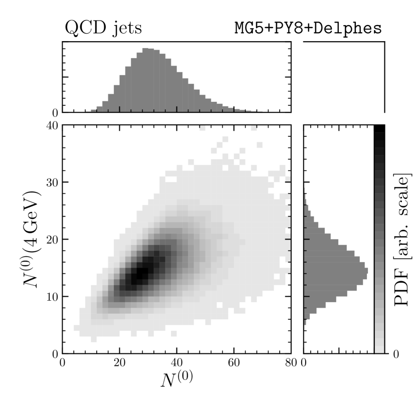
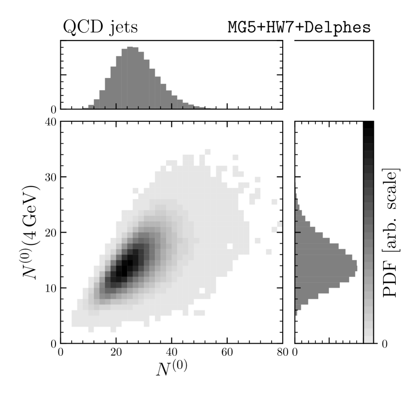
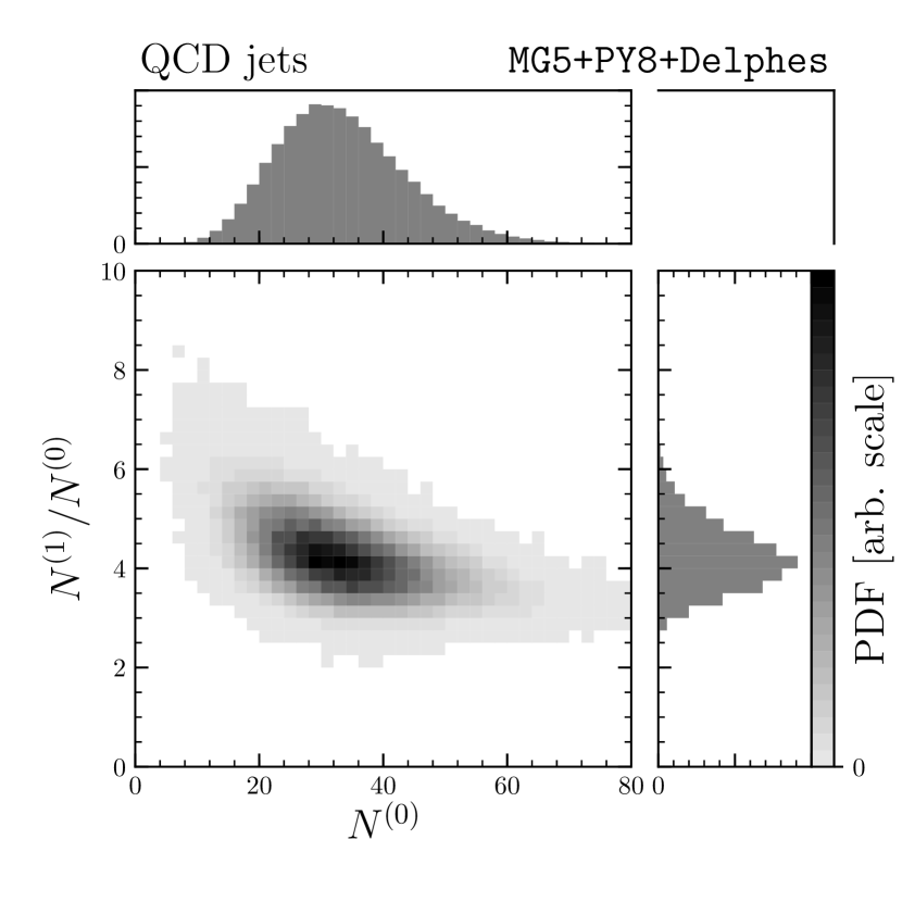
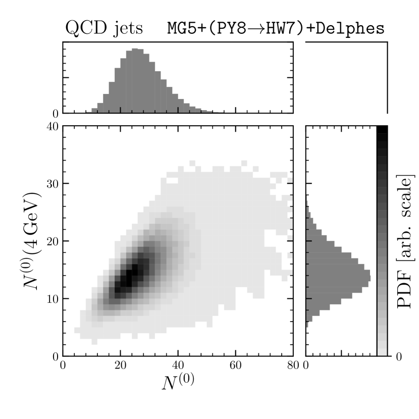
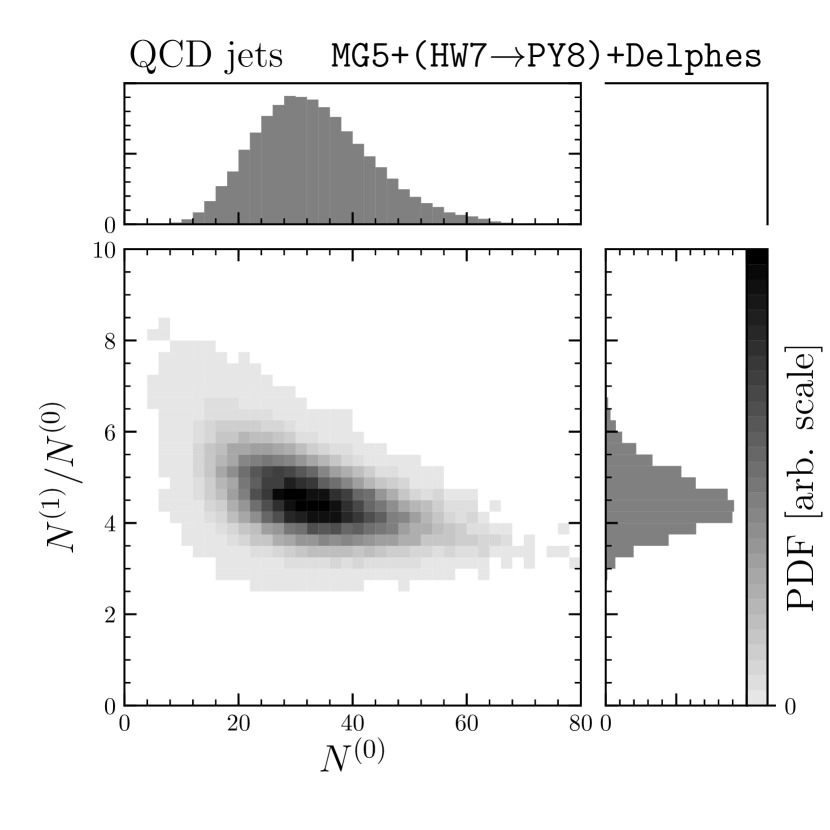
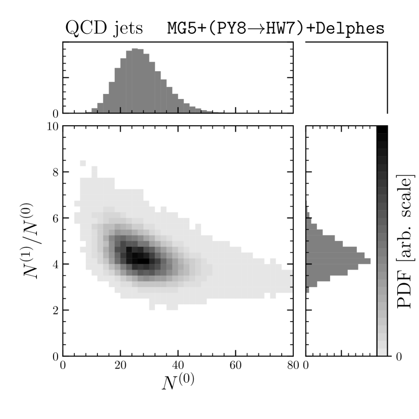
In figure 17, we show the $(N^{(0)},N^{(0)}(4\,\mathrm{GeV}))$ distributions of the QCD jet samples. The $N^{(0)}$ distribution simulated by PY8 is broader than that simulated by HW7. The tail of the $N^{(0)}$ distribution exceeds 60 for PY8, but it vanishes at there for HW7. On the other hand, the $N^{(0)}(4\,\mathrm{GeV})$ distributions of PY8 and HW7 are similar, as shown in figure 10. The active pixels with $p_{T}>4\,\mathrm{GeV}$ correspond to the particles from high $p_{T}$ partons in the shower. Predictions on those partons in the two generators tend to agree, and the predicted $N^{(0)}(4\,\mathrm{GeV})$ distributions are also similar. The $N^{(1)}/N^{(0)}$ distributions of PY8 and HW7 are also similar, as shown in figure 18. Therefore, $N^{(0)}$ should play an important role in the classification.

(a)

(b)

Figure 17: $(N^{(0)},N^{(0)}(4\,\mathrm{GeV}))$ distributions for (a) PY8 and (b) HW7

(a)

(b)

Figure 18: $(N^{(0)},N^{(1)}/N^{(0)})$ distributions for (a) PY8 and (b) HW7

The separation of the top jets and QCD jets is worse for HW7 compared with PY8 discussed in previous sections. The AUC of the top jet vs. QCD jet classification predicted by HW7 is smaller than that predicted by PY8. In figure 19, we show the ROC curves of each classifier trained on HW7 events. The performance of the $\mathrm{RN}_{S_{2}}$ is similar to that trained on PY8 events. Once $N^{(0)}$ is additionally considered in the classification, the performance is improved. However, the improvement from adding $N^{(0)}$ is significantly smaller in HW7, because the $N^{(0)}$ distributions of top jets and QCD jets are close, as shown in figure 10.

Figure 19: The ROC curves of the networks trained on HW7 samples.

In the previous analysis, we have shown that inputs $N^{(0)}$, $N^{(0)}(4\,\mathrm{GeV})$, $N^{(1)}$, and $N^{(1)}(4\,\mathrm{GeV})$ in addition to $S_{2,ab}$ is good enough for building a neural network that fits the CNN output. At the same time, this indicates that tuning of the event generator focusing on these counting variables can be an efficient way to obtain the simulated data that gives consistent results with the experimental data.

If the difference between the simulated and experimental data is not too large, reweighting simulated events is useful for reducing the difference. We consider reweighting based on the marginal distribution of interested variables $\bm{x}$. Let $\rho_{\mathrm{true}}(\bm{x})$ and $\rho_{\mathrm{MC}}(\bm{x})$ be the $\bm{x}$ distributions with true and simulated events, respectively. The new weight $w_{\mathrm{new}}^{[i_{Y}]}$ of the event $i_{Y}$ is given as follows,

$$w_{\mathrm{new}}^{[i_{Y}]}=\frac{\rho_{\mathrm{true}}(\bm{x}^{[i_{Y}]})}{\rho_{\mathrm{MC}}(\bm{x}^{[i_{Y}]})}\cdot w_{\mathrm{old}}^{[i_{Y}]},$$ (51)

where $w_{\mathrm{old}}^{[i_{Y}]}$ is the weight before reweighting.

Let us perform an exercise to correct $(N^{(0)},N^{(0)}(4\,\mathrm{GeV}))$ distribution, assuming that either one of the distributions $\rho_{\texttt{PY8}{}}$ and $\rho_{\texttt{HW7}{}}$ simulated by PY8 and HW7 is $\rho_{\mathrm{true}}$ while the other is $\rho_{\mathrm{MC}}$. We consider the reweighting of these two variables in order to consider a non-trivial case that some of the variables are correlated. The reweighting factor ${\rho_{\mathrm{true}}(N^{(0)},N^{(0)}(4\,\mathrm{GeV}))}/{\rho_{\mathrm{MC}}(N^{(0)},N^{(0)}(4\,\mathrm{GeV}))}$ is calculated using the normalized histogram of $(N^{(0)},N^{(0)}(4\,\mathrm{GeV}))$, as stated in appendix E. The $N^{(1)}$ distribution in figure 20 still disagree after the reweighing, but the deviation is minor. Because the sample size is limited, we do not attempt to correct all those distribution in this paper.

Figure 20: The $N^{(1)}$ and $N^{(1)}(4\,\mathrm{GeV})$ distributions of PY8, HW7, and reweighted HW7 samples.

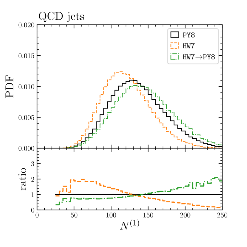
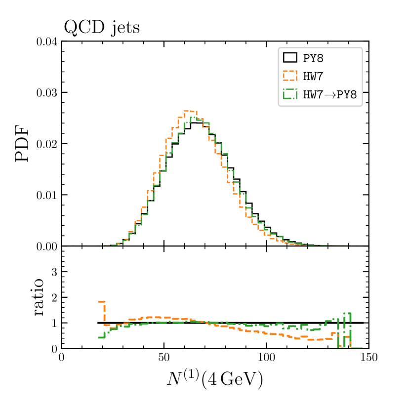
Figure 21 shows the $\hat{y}^{0}$ distributions for QCD jet samples, of the models trained on PY8 samples. The orange dashed, black solid, and green dot-dashed histograms are the $\hat{y}^{0}$ distributions with HW7, PY8, and reweighted HW7 samples, respectively.

Figure 21(a) shows the $\hat{y}^{0}$ distributions of $\mathrm{RN}_{S_{2}}$. This classifier does not use $N^{(0)}$ and $N^{(0)}(4\,\mathrm{GeV})$ explicitly, but the distribution of reweighted HW7 samples comes quite close to that of PY8 samples. The score difference comes from the difference of $S_{2}$ distribution. The $S_{2,\mathrm{soft}}$ distribution of HW7 samples is 10% smaller than that of PY8 samples. The reweighting reduces the difference because $N^{(0)}$ and $S_{2,\mathrm{soft}}$ are correlated. The Pearson correlation coefficient between $N^{(0)}$ and $S_{2,\mathrm{soft}}^{(i)}$ is 0.3 for both PY8 and HW7. The bin-by-bin ratio of the average $\langle S_{2,\mathrm{soft}}^{(i)}\rangle$ between HW7 and PY8 samples is about 0.9. The average $\langle S_{2,\mathrm{soft}}^{(i)}\rangle$ of HW7 samples increases after the reweighting and the $S_{2,\mathrm{soft}}$ distributions get closer to each other. On the other hand, the reweighting increases the disagreement of $p_{T,\mathbf{J}}$ distribution. The sum of the weights of the reweighted HW7 samples with $p_{T,\mathbf{J}}\sim 500\,\mathrm{GeV}$ is about 20% larger than that of PY8 samples. We marginalized $p_{T,\mathbf{J}}$ during the training so that the impact on the $\hat{y}^{0}$ distribution is minimal. Therefore, the agreement seen in figure 21(a) is mainly due to the correction of $S_{2,ab}$, and it is encouraging.

(a)

(b)

(c)

(d)

Figure 21: The $\hat{y}^{0}$ distributions of PY8 and HW7 test samples for the model trained on the PY8 events. The neural networks used in the plots are (a) $\mathrm{RN}_{S_{2}}$, (b) $\mathrm{RN}_{S_{2},N^{(0)},N^{(0)}(4\,\mathrm{GeV})}$, (c) $\mathrm{RN}_{S_{2},N^{(0)},N^{(1)}}$, and (d) $\mathrm{CNN}$.

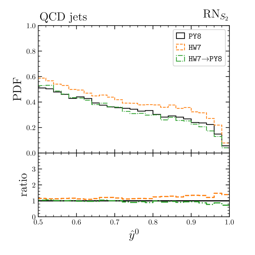
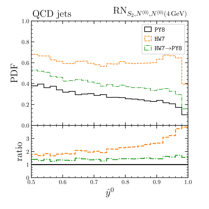
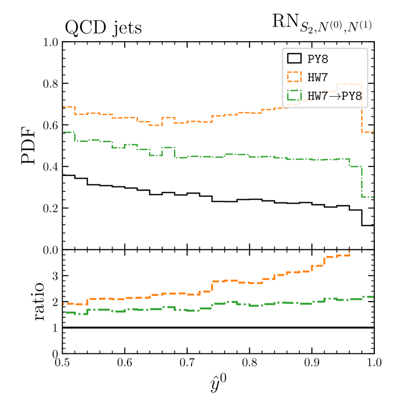
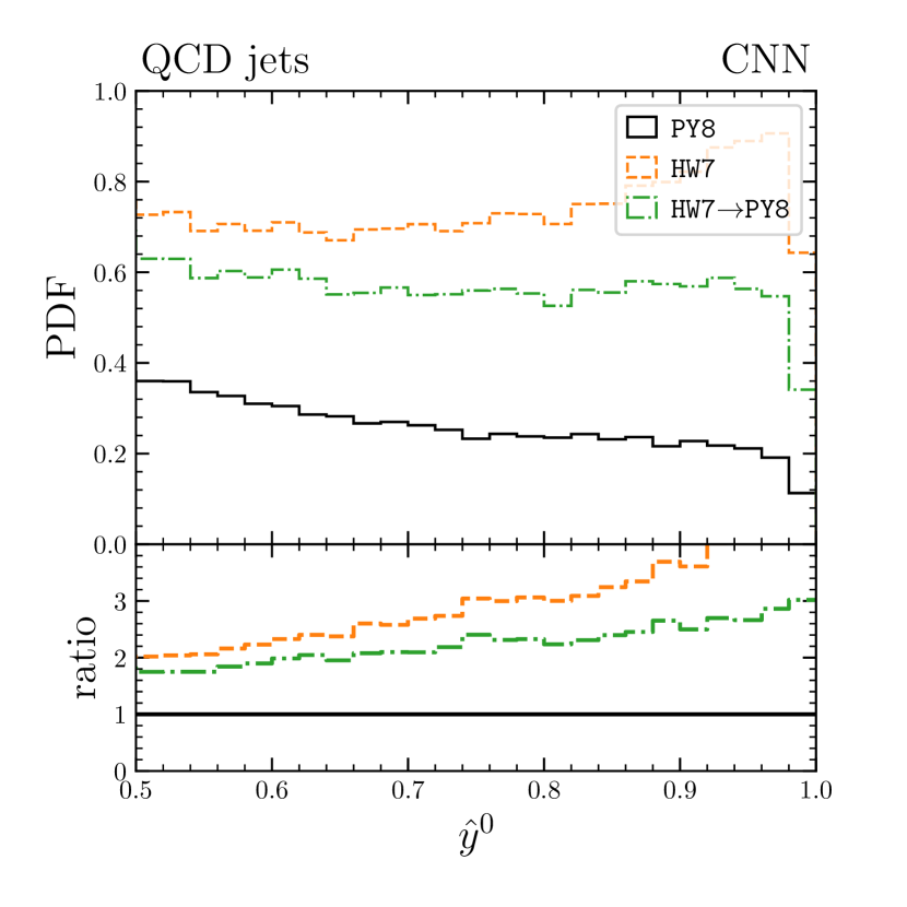
Figure 21(b) shows the $\hat{y}^{0}$ distributions of $\mathrm{RN}_{S_{2},N^{(0)},N^{(0)}(4\,\mathrm{GeV})}$. For $\hat{y}^{0}\sim 1$, the ratio of the $\hat{y}^{0}$ distributions of HW7 and PY8 exceeds 4, and the distribution of HW7 samples even peaks near $\hat{y}^{0}\sim 1$. This means that the model trained on PY8 samples focuses on a particular region in order to get high purity top samples, but the HW7 samples are still populated in the region. In the situation that the HW7 distribution is “true” while PY8 samples are used to build the top jet vs. QCD jet classifier, we overestimate the top quark event rate by dijet contamination; adding the variables whose “true distributions” are not well understood could cause the problem of this kind.

The ratio between weighted HW7 and PY8 distributions is constant. This is nice in order to avoid the systematics along with tightening the cut to reject QCD events. On the other hand, the ratio of the reweighted HW7 samples is much larger than that in figure 21(a). The deviation should come from the mismodeling of the correlation between $N^{(0)}$ and other parameters. The difference is even larger if one includes $N^{(1)}$ in the inputs, as shown in figure 21(c). The ratio between the weighted HW7 and PY8 sample is now nearly a factor of two larger at $y\sim 1$ and even increasing. This disagreement is not surprising given the very poor sample of HW7 in the high $N^{(0)}$ region. Finally, figure 21(d) is the $\hat{y}^{0}$ distribution of the CNN model. The distributions looks quite similar to those in figure 21(c) before reweighting, but the ratio of the distributions of reweighted HW7 events and PY8 events is larger than that of $\mathrm{RN}_{S_{2},N^{(0)},N^{(1)}}$.

Figure 22 shows the $\hat{y}^{0}$ distributions of the model $\mathrm{RN}_{S_{2},N^{(0)},N^{(0)}(4\,\mathrm{GeV})}$ trained on HW7 events. Recall that the QCD jets in PY8 samples cover the phase space of the QCD jets simulated by HW7, and the reweighting is then effective for transforming the PY8 samples to HW7 samples. The opposite is not true because there are QCD jets which are not in HW7 generated samples. The reweighting is not exact because we have only a small number of events in some phase space region, and we see some deviation in $\hat{y}$ distribution, as shown in figure 21(b). If one wishes to describe real data by assigning an appropriate weight for each simulated events, it is better to use a generator setup that covers wider phase space so that we can correct the event distribution by using experimental data afterwords.

Figure 22: The score distribution of PY8 and HW7 test sample for the model trained by the HW7 events.

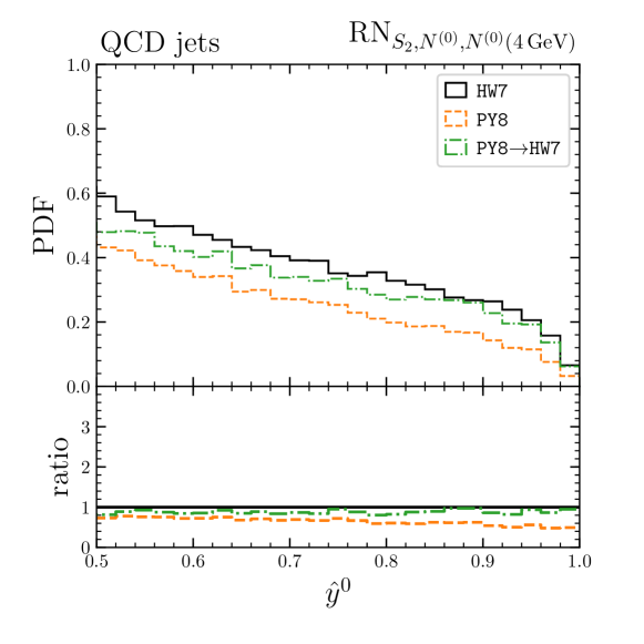
The disagreement between PY8 and HW7 samples remains after the reweighting in this exercise. We do not proceed to reweight distributions other than the $(N^{(0)},N^{(0)}(4\,\mathrm{GeV}))$ distribution in this paper because of the statistical limitation. Neural network-based reweighing Andreassen:2019nnm can be helpful for adjusting full phase-space, but it is beyond the scope of this paper. The difference between the two generators is too large to achieve perfect agreement simply by reweighting. Because $N^{(0)}$ and $N^{(1)}$ are important quantities for describing the neural network-based classifier, those generators may be tuned carefully to reproduce the distribution of soft activities in jet images.

6 Discussions

In this paper, we have identified essential quantities that the CNN on a jet image is using for the top jet vs. QCD jet classification. The discovered quantities consist of both IRC safe and IRC unsafe observables. The former includes the IRC safe two-point energy correlation, jet spectrum, as a function of the distance between two jet constituents. The latter is an IRC unsafe Minkowski sequence inspired from the Minkowski functionals that describes morphological information on the set of jet constituents. It gives a quantitative measure of the area that is occupied by the particles inside jets. The first element of the Minkowski sequence is the number of active pixels in the jet image, $N^{(0)}$, and the second element $N^{(1)}$ is the sum of the $N^{(0)}$ and the number of the pixels adjacent to the active pixels. These quantities are derivable from a jet image, and the relation network (RN) trained on these quantities (along with kinematic observables) has equivalent performance to the CNN.

The IRC safe quantities are theoretically more controlled, especially different event simulators predict consistent distributions. On the other hand, the IRC unsafe quantities are described by phenomenological models tuned by the experimental data. The classification performance of RN agrees with that of CNN only when we include IRC unsafe Minkowski sequences among the inputs. The similarity of the performance indicates that the top jet classifier based on CNN uses the geometric information of soft radiation, and we have succeeded in reproducing the CNN predictions using fewer degrees of freedom.

We also point out that the training of the RN is more stable than the CNN. The stability comes from the fact that the RN classifiers use a restricted set of derived inputs from the jet images, and the loss function of the RN is less complicated than that of CNN. We measure the variation of the training results by randomly swapping the event orders in the batch training and using a different initial parameter in the networks. The variation of the RN output is about factor 3 smaller than that of the CNN output, as we have seen in table 2.

As the IRC safe inputs, we choose the jet spectrum Lim:2018toa ; Chakraborty:2019imr , which is aggregated two-point energy correlation as the function of the $\Delta R$. We introduce the various improvements on the jet spectrum from the previous paper. In this paper, it is derived from a constrained graph network. A vertex of the graph network corresponds to a jet constituent, while each vertex carries information of the constituent momentum and the subjet ID to which the constituent belongs. The edges links between two vertices and represent the two-point correlation between the two constituents. For the classification of top jets and QCD jets, we find that the correlation among the trimmed jet and the correlation between the leading subjet and the other constituents, and their geometry are especially useful in the classification. We systematically include the three-point structure of the top quark in the two-point energy correlations after removing the leading subjet. The modularized networks process the two-point correlations separately with global kinematical inputs so that the combined network accepts significantly more inputs without inflating the parameters in the hidden layers.

The classifiers using the IRC unsafe quantities, such as soft pixels of jet image or the Minkowski sequence, could suffer from systematic uncertainties of the simulation. After the identification of the key morphological quantities, we can minimize efforts on calibration by focusing on the $N^{(0)}$ and $N^{(1)}$ distributions. The distributions may be corrected relatively easily by reweighting events to calibrate the distributions to the observed data. We demonstrate that the reweighting of the simulated events to reproduce the true $N^{(0)}$ distributions greatly reduce the systematic error of the classifiers. Such tuning of the data reduces the systematic uncertainties in the ML classifications that depend on the simulated events.

In summary, we propose an approach to replace a complex neural network using the low level inputs into a simple network using the processed inputs motivated from a physics point of view. To this end, we show surprising evidence that the CNN output depends on the geometrical measures expressed by discritized version of the Minkowski functionals. These morphological quantities improve jet classification significantly. The study of jet morphology from the data, and comparison to the prediction from event simulation might be an exciting direction to persuade. We think the variables may be further extended not only for jet physics but also for the analysis of event geometry or anomaly searches.

Appendix A Setup for Monte-Carlo Event Simulation

We generate $pp\rightarrow t\bar{t}$ and $pp\rightarrow jj$ events for top jet and QCD jet samples, respectively. The symbol $j$ represents gluon or (anti-)quark other than the top quark. The parton level events are generated by Madgraph5 2.6.6 Alwall:2014hca . The center of mass energy is 13 TeV. Produced top quarks are forced to decay into $bW$ and the subsequent $W$ boson decays into two quarks including $b$-quarks. Since we are only interested in boosted top quarks, we generate events with outgoing partons whose $p_{T}$ is larger than 450 GeV. Numbers of the generated $pp\rightarrow t\bar{t}$ and $pp\rightarrow jj$ events with this preselection are 5 million and 10 million, respectively. The renormalization and factorization scales are set to be $H_{T}/2$, where $H_{T}$ is the sum of the transverse energy of each parton, and the parton distribution function is NNPDF23_lo_as_0130_qed Ball:2012cx ; Ball:2013hta ; Carrazza:2013bra ; Carrazza:2013wua . Two parton shower and hadronization simulations are considered in this paper: Pythia 8.226 Sjostrand:2014zea with Monash tune Skands:2014pea and Herwig 7.1.3 Bellm:2015jjp ; Bahr:2008pv with default tune herwigtune ; Gieseke:2012ft . The pile-ups are not included but the underlying events and multi-parton interactions are considered.

We use Delphes 3.4.1 deFavereau:2013fsa for detector simulation with its default ATLAS detector configuration. Jets are reconstructed from calorimeter towers whose $(\eta,\phi)$ resolutions at electromagnetic and hadronic calorimeters in $|\eta|<2.5$ are assumed to be (0.0174,$1^{\circ}$) and (0.1, $10^{\circ}$), respectively. Anti-$k_{T}$ jet clustering algorithm Cacciari:2008gp with radius parameter $R_{\mathbf{J}}=1.0$ implemented in fastjet 3.3.0 Cacciari:2011ma ; Cacciari:2005hq is used to cluster these calorimeter towers into jets. The leading $p_{T}$ jets with its transverse momentum $p_{T,\mathbf{J}}\in[500,600]$ GeV and mass $m_{\mathbf{J}}\in[150,200]$ GeV are selected for the analysis. In addition, a top jet sample is required to have quarks from the originating top quark within $R_{\mathbf{J}}$ from the jet axis. After this selection, we have about 950,000 top jets and 350,000 QCD jets. Half of them are used for the training and th others are used for testing. For jet trimming, we use $k_{T}$ algorithm Catani:1993hr ; Ellis:1993tq with radius 0.2 and keep subjets whose energy fraction is larger than 0.05. The leading $p_{T}$ subjet $\mathbf{J}_{1}$ is the highest $p_{T}$ anti-$k_{T}$ subjet Cacciari:2008gp with radius 0.2.

Note that we have not used matched sample, so that the modeled $p_{T,\mathbf{J}}$ distribution is not precise beyond the leading order accuracy. Nevertheless, the changes due to recoiling from extra radiation are not a main interest in this paper, so we use this samples by presuming that the top jets and QCD jets are factorizable.

Appendix B Kernel Density Estimation of $p_{T,\mathbf{J}}$ Distribution

We use the kernel density estimation (KDE) on a finite interval $[p_{T,\mathbf{J}}^{\min},p_{T,\mathbf{J}}^{\max}]$ to model the event-by-event weight $f_{p_{T,\mathbf{J}}}(p_{T,\mathbf{J}};Y)$ in eq. (45). First, we transform $p_{T\,jet}$ into a logit $t(p_{T,\mathbf{J}})$ in order to make the domain unbounded.

$$t(p_{T,\mathbf{J}})={\mathrm{logit}}\left(\frac{p_{T,\mathbf{J}}-p_{T,\mathbf{J}}^{\min}}{p_{T,\mathbf{J}}^{\max}-p_{T,\mathbf{J}}^{\min}}\right)=-\log\frac{p_{T,\mathbf{J}}-p_{T,\mathbf{J}}^{\min}}{p_{T,\mathbf{J}}^{\max}-p_{T,\mathbf{J}}}$$ (52)

The KDE of the sampled logits, $t(p_{T,\mathbf{J}}^{[i_{N_{Y}}]})$ is used to estimate the probability density function $f_{P_{T,\mathbf{J}}}(p_{T,\mathbf{J}};Y)$.

$$f_{P_{T,\mathbf{J}}}(p_{T,\mathbf{J}};Y)\approx\frac{t^{\prime}(p_{T,\mathbf{J}})}{N_{Y}}\sum_{i_{Y}=1}^{N_{Y}}K_{h}(t(p_{T,\mathbf{J}})-t(p_{T,\mathbf{J}}^{[i_{Y}]})),\quad t^{\prime}(p_{T,\mathbf{J}})=\frac{p_{T,\mathbf{J}}^{\max}-p_{T,\mathbf{J}}^{\min}}{(p_{T,\mathbf{J}}^{\max}-p_{T,\mathbf{J}})(p_{T,\mathbf{J}}-p_{T,\mathbf{J}}^{\min})}$$ (53)

where $K_{h}$ is a scaled kernel whose bandwith parameter is $h$. In particular, a gaussian kernel with bandwith $h=0.25$ is used for the KDE.

$$K_{h}(x)=\frac{1}{h}K\left(\frac{x}{h}\right),\quad K(x)=\frac{1}{\sqrt{2\pi}}\exp\left(-\frac{x^{2}}{2}\right)$$ (54)

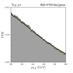
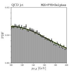
However, $t^{\prime}(p_{T,\mathbf{J}})$ is singular at $p_{T,\mathbf{J}}^{\min}$ and $p_{T,\mathbf{J}}^{\max}$, and the estimation of the probability density near the boundary is less precise. Instead of using samples after the selection $p_{T,\mathbf{J}}\in[500,600]$ GeV, we use a selection with broader $p_{T,\mathbf{J}}$ range, $[450,650]$ GeV for KDE only in order to avoid the effects from the singularities. The KDE is then normalized for $p_{T,\mathbf{J}}\in[500,600]$ GeV afterward. We show the normalized histogram of $p_{T,\mathbf{J}}$ and the KDE in figure 23.

Figure 23: The histogram and modeled probability density distribution of $p_{T,\mathbf{J}}$ for (left) top jet samples and (right) QCD jet samples. Solid black line is the KDE. The vertical bar is the statistical uncertainty of each bin. The green and yellow bands are pointwise statistical uncertainty of the KDE calculated from squared sum of the summands.

Appendix C Network Implementations

C.1 Relation Networks

The relation networks used in this paper are implemented as follows. The module for analyzing the energy correlation with jet trimming, $\bm{h}_{\mathrm{trim}}=\mathrm{MLP}_{\mathrm{trim}}(\bm{x}_{\mathrm{trim}},\bm{x}_{\mathrm{kin}})$, consists of two hidden layers,

$$\bm{h}^{(1)}_{\mathrm{trim}} = \mathrm{FC}(\bm{z}_{\mathrm{trim}},\bm{z}_{\mathrm{kin}})$$ , size: 200, activation: ELU

$$\bm{h}^{(2)}_{\mathrm{trim}} = \mathrm{FC}(\bm{h}^{(1)}_{\mathrm{trim}})$$ , size: 200, activation: ELU

$$\bm{h}_{\mathrm{trim}} = \mathrm{FC}(\bm{h}^{(2)}_{\mathrm{trim}})$$ , size: 5, activation: linear (55)

where $\bm{z}_{i}$ is the standardized inputs of $\bm{x}_{i}$, and $\mathrm{FC}$ is a fully-connected layer with a given output size and activation function. Note that we do not apply $L_{2}$ regularization for the $\mathrm{FC}$s with linear activation. The module for analyzing the energy correlation of $\mathbf{J}_{1}$ and $\mathbf{J}\setminus\mathbf{J}_{1}$ is as follows.

$$\bm{h}^{(1)}_{\mathbf{J}_{1}} = \mathrm{FC}(\bm{z}_{\mathbf{J}_{1}},\bm{z}_{\mathrm{kin}})$$ , size: 200, activation: ELU

$$\bm{h}^{(2)}_{\mathbf{J}_{1}} = \mathrm{FC}(\bm{h}^{(1)}_{\mathbf{J}_{1}})$$ , size: 200, activation: ELU

$$\bm{h}_{\mathbf{J}_{1}} = \mathrm{FC}(\bm{h}^{(2)}_{\mathbf{J}_{1}})$$ , size: 5, activation: linear (56)

The logits $\bm{u}^{\prime}$ for the binary classification is implemented as follows.

$$\bm{h}^{(1)}_{{\mathrm{logit}}} = \mathrm{FC}(\bm{h}_{\mathrm{trim}},\bm{h}_{\mathbf{J}_{1}},\bm{z}_{\mathrm{kin}})$$ , size: 200, activation: ELU

$$\bm{h}^{(2)}_{{\mathrm{logit}}} = \mathrm{FC}(\bm{h}^{(1)}_{{\mathrm{logit}}})$$ , size: 200, activation: ELU

$$\bm{u}^{\prime} = \mathrm{FC}(\bm{h}^{(2)}_{{\mathrm{logit}}})$$ , size: 2, activation: linear (57)

For the relation networks with inputs $\bm{x}_{\mathrm{geometry}}$, we replace $\bm{h}^{(1)}_{{\mathrm{logit}}}$ of eq. (C.1) as follows.

$$\bm{h}^{(1)}_{{\mathrm{logit}}} = \makebox[0.0pt][l]{ $\mathrm{FC}(\bm{h}_{\mathrm{trim}},\bm{h}_{\mathbf{J}_{1}},\bm{z}_{\mathrm{geometry}})$, }\phantom{000000000000000000000000}\makebox[0.0pt][l]{ size: 200, }\phantom{00000000000}\textrm{activation: ELU},$$ (58)

C.2 Convolutional Neural Networks

Our convolutional neural networks are trained on the preprocessed jet images obtained as in Chakraborty:2019imr . We recluster given jet constituents by $k_{T}$ algorithm Catani:1993hr ; Ellis:1993tq with radius parameter $R_{\mathbf{J}}=0.2$ and translate the $(\eta,\phi)$ coordinate so that the leading $p_{T}$ subjet axis is at $(0,0)$. If a subleading $p_{T}$ subjet exists, we rotate the $(\eta,\phi)$ corordinate about the origin so that the subjet is on the positive $y$-axis on the rotated coordinate. If a third leading $p_{T}$ subjet exists with a negative $x$ coordinate, we reflect the coordinate to across the $y$ axis so that the third leading $p_{T}$ subjet always has a positive $x$ coordinate. The preprocessed jet image $\bm{x}_{\mathrm{image}}$ is a two-dimensional $p_{T}$-weighted histogram of those regularized constituents on a range $[-1.5,1.5]\otimes[-1.5,1.5]$ with bin size $0.1\times 0.1$. The energy deposit of each pixel is standardized thereafter.

The vanilla CNN of this paper consists of six convolutional layers with a filter size $3\times 3$. The standardized image $\bm{z}_{\mathrm{image}}$ of $\bm{x}_{\mathrm{image}}$ is fed into a chain of convolutional layers as follows.

$$\bm{h}^{(1)}_{\mathrm{CNN}} = \makebox[0.0pt][l]{ $\mathrm{CONV}(\bm{z}_{\mathrm{image}})$, }\phantom{0000000000000000000}\makebox[0.0pt][l]{ size: $30\times 30\times 16$, }\phantom{000000000000000000}\makebox[0.0pt][l]{ filter size: $3\times 3$, }\phantom{00000000000000000}\textrm{activation: ELU},$$

$$\bm{h}^{(2)}_{\mathrm{CNN}} = \makebox[0.0pt][l]{ $\mathrm{CONV}(\bm{h}^{(1)}_{\mathrm{CNN}})$, }\phantom{0000000000000000000}\makebox[0.0pt][l]{ size: $30\times 30\times 16$, }\phantom{000000000000000000}\makebox[0.0pt][l]{ filter size: $3\times 3$, }\phantom{00000000000000000}\textrm{activation: ELU},$$

$$\bm{h}^{(3)}_{\mathrm{CNN}} = \makebox[0.0pt][l]{ $\mathrm{CONV}(\bm{h}^{(2)}_{\mathrm{CNN}})$, }\phantom{0000000000000000000}\makebox[0.0pt][l]{ size: $30\times 30\times 16$, }\phantom{000000000000000000}\makebox[0.0pt][l]{ filter size: $3\times 3$, }\phantom{00000000000000000}\textrm{activation: ELU},$$

$$\bm{h}^{(3,\mathrm{POOL})}_{\mathrm{CNN}} = \mathrm{POOL}(\bm{h}^{(3)}_{\mathrm{CNN}}) 15\times 15\times 16 2\times 2$$ , size: , pool size: ,

$$\bm{h}^{(4)}_{\mathrm{CNN}} = \makebox[0.0pt][l]{ $\mathrm{CONV}(\bm{h}^{(3,\mathrm{POOL})}_{\mathrm{CNN}})$, }\phantom{0000000000000000000}\makebox[0.0pt][l]{ size: $15\times 15\times 8$, }\phantom{000000000000000000}\makebox[0.0pt][l]{ filter size: $3\times 3$, }\phantom{00000000000000000}\textrm{activation: ELU},$$

$$\bm{h}^{(5)}_{\mathrm{CNN}} = \makebox[0.0pt][l]{ $\mathrm{CONV}(\bm{h}^{(4)}_{\mathrm{CNN}})$, }\phantom{0000000000000000000}\makebox[0.0pt][l]{ size: $15\times 15\times 8$, }\phantom{000000000000000000}\makebox[0.0pt][l]{ filter size: $3\times 3$, }\phantom{00000000000000000}\textrm{activation: ELU},$$

$$\bm{h}^{(6)}_{\mathrm{CNN}} = \makebox[0.0pt][l]{ $\mathrm{CONV}(\bm{h}^{(5)}_{\mathrm{CNN}})$, }\phantom{0000000000000000000}\makebox[0.0pt][l]{ size: $15\times 15\times 8$, }\phantom{000000000000000000}\makebox[0.0pt][l]{ filter size: $3\times 3$, }\phantom{00000000000000000}\textrm{activation: ELU},$$

$$\bm{h}^{(6,\mathrm{POOL})}_{\mathrm{CNN}} = \mathrm{POOL}(\bm{h}^{(6)}_{\mathrm{CNN}}) 7\times 7\times 8 2\times 2$$ , size: , pool size: ,

$$\bm{h}^{(7)}_{\mathrm{CNN}} = \makebox[0.0pt][l]{ $\mathrm{FC}(\bm{h}^{(6,\mathrm{POOL})}_{\mathrm{CNN}})$, }\phantom{0000000000000000000}\makebox[0.0pt][l]{ size: $200$, }\phantom{000000000000}\textrm{activation: ELU},$$

$$\bm{h}_{\mathrm{CNN}} = \makebox[0.0pt][l]{ $\mathrm{FC}(\bm{h}^{(7)}_{\mathrm{CNN}})$, }\phantom{0000000000000000000}\makebox[0.0pt][l]{ size: $100$, }\phantom{000000000000}\textrm{activation: linear},$$ (59)

where $\mathrm{CONV}$ is a two-dimensional convolutional layer with a given filter size and activation function, and $\mathrm{POOL}$ is a max-pooling layer with a given pool size. The output size consists of three numbers: the first two numbers represent output image width and height, and the third number is the number of filters. We simply put $\bm{h}_{\mathrm{CNN}}$ to $\mathrm{MLP}_{{\mathrm{logit}}}$ by replacing eq. (C.1) to the following.

$$\bm{h}^{(1)}_{{\mathrm{logit}}} = \mathrm{FC}(\bm{h}_{\mathrm{CNN}},\bm{z}_{\mathrm{kin}})$$ , size: 200, activation: ELU (60)

The ResNet in section 4.4 consists of convolutional layers $\bm{h}^{(i+1,\mathrm{res})}_{\mathrm{ResNet}}$ with skip connection $\bm{h}^{(i+1,\mathrm{shortcut})}_{\mathrm{ResNet}}$. We define a ResNet module of input image $\bm{h}^{(i)}_{\mathrm{ResNet}}$ as follows.

$$\bm{h}^{(i+1,\mathrm{res})}_{\mathrm{ResNet}} = \mathrm{CONV}\circ\mathrm{ELU}\circ\mathrm{CONV}(\bm{h}^{(i)}_{\mathrm{ResNet}})$$ ,

$$\bm{h}^{(i+1,\mathrm{shortcut})}_{\mathrm{ResNet}} = \begin{cases}\bm{h}^{(i)}_{\mathrm{ResNet}}&\textrm{if $\bm{h}^{(i)}_{\mathrm{ResNet}}$ and $\bm{h}^{(i+1)}_{\mathrm{ResNet}}$ has the same size, }\\ \mathrm{CONV}_{1\times 1}(\bm{h}^{(i)}_{\mathrm{ResNet}})&\textrm{otherwise,}\end{cases}$$

$$\bm{h}^{(i+1)}_{\mathrm{ResNet}} = \mathrm{ResNet}(\bm{h}^{(i)}_{\mathrm{ResNet}})=\mathrm{ELU}(\bm{h}^{(i+1,\mathrm{res})}_{\mathrm{ResNet}}+\bm{h}^{(i+1,\mathrm{shortcut})}_{\mathrm{ResNet}})$$ (61)

where $\mathrm{CONV}_{1\times 1}$ is a convolutional layer with filter size $1\times 1$. The hyperparameters of other $\mathrm{CONV}$ will be specified later. All the convolutional operations above do not have any activation function. If input image size and output image size are different, we use strided convolution on $\mathrm{CONV}(\bm{h}^{(i)}_{\mathrm{ResNet}})$. We build a ResNet by replacing the chain of convolutional layers in eq. (59) to the following chain of six ResNet modules.

$$\bm{h}^{(1)}_{\mathrm{ResNet}} = \mathrm{ResNet}(\bm{z}_{\mathrm{image}}) 30\times 30\times 16 3\times 3$$ , size: , filter size: ,

$$\bm{h}^{(2)}_{\mathrm{ResNet}} = \mathrm{ResNet}(\bm{h}^{(1)}_{\mathrm{ResNet}}) 30\times 30\times 16 3\times 3$$ , size: , filter size: ,

$$\bm{h}^{(3)}_{\mathrm{ResNet}} = \mathrm{ResNet}(\bm{h}^{(2)}_{\mathrm{ResNet}}) 15\times 15\times 8 3\times 3$$ , size: , filter size: , stride: 2,

$$\bm{h}^{(4)}_{\mathrm{ResNet}} = \mathrm{ResNet}(\bm{h}^{(3)}_{\mathrm{ResNet}}) 15\times 15\times 8 3\times 3$$ , size: , filter size: ,

$$\bm{h}^{(5)}_{\mathrm{ResNet}} = \mathrm{ResNet}(\bm{h}^{(4)}_{\mathrm{ResNet}}) 8\times 8\times 8 3\times 3$$ , size: , filter size: , stride: 2,

$$\bm{h}^{(6)}_{\mathrm{ResNet}} = \mathrm{ResNet}(\bm{h}^{(5)}_{\mathrm{ResNet}}) 8\times 8\times 8 3\times 3$$ , size: , filter size: ,

$$\bm{h}^{(1)}_{{\mathrm{logit}}} = \mathrm{FC}(\bm{h}^{(6)}_{\mathrm{ResNet}},\bm{z}_{\mathrm{kin}})$$ , size: 200, activation: ELU. (62)

The ResNeXt in section 4.4 uses multiple chains of convolutional layers for the residual learning parts $\bm{h}_{\mathrm{ResNet}}^{(i+1,\mathrm{res})}$ in the ResNet. The ResNeXt module with four parallel chains of convolutional layers is defined as follows.

$$\bm{h}^{(i+1,j)}_{\mathrm{ResNeXt}} = \mathrm{ELU}\circ\mathrm{CONV}\circ\mathrm{ELU}\circ\mathrm{CONV}_{1\times 1}(\bm{h}^{(i)}_{\mathrm{ResNeXt}}),$$

$$\bm{h}^{(i+1,\mathrm{res})}_{\mathrm{ResNeXt}} = \mathrm{CONV}_{1\times 1}\left(\bigoplus_{j=1}^{4}\bm{h}^{(i+1,j)}_{\mathrm{ResNeXt}}\right),$$

$$\bm{h}^{(i+1,\mathrm{shortcut})}_{\mathrm{ResNeXt}} = \mathrm{CONV}_{1\times 1}(\bm{h}^{(i)}_{\mathrm{ResNeXt}}),$$

$$\bm{h}^{(i+1)}_{\mathrm{ResNet}} = \mathrm{ResNeXt}(\bm{h}^{(i)}_{\mathrm{ResNeXt}})=\mathrm{ELU}\left(\bm{h}^{(i+1,\mathrm{res})}_{\mathrm{ResNeXt}}+\bm{h}^{(i+1,\mathrm{shortcut})}_{\mathrm{ResNeXt}}\right),$$ (63)

where the direct sum of the images represents a stacked image along the filter dimension. Since we use many convolutional layers already, we use three of those modules for the image analyzer.

$$\bm{h}^{(1)}_{\mathrm{ResNeXt}} = \mathrm{ResNeXt}(\bm{z}_{\mathrm{image}}) 30\times 30\times 16 3\times 3$$ , size: , filter size: ,

$$\bm{h}^{(2)}_{\mathrm{ResNeXt}} = \mathrm{ResNeXt}(\bm{h}^{(1)}_{\mathrm{ResNeXt}}) 30\times 30\times 16 3\times 3$$ , size: , filter size: ,

$$\bm{h}^{(3)}_{\mathrm{ResNeXt}} = \mathrm{ResNeXt}(\bm{h}^{(2)}_{\mathrm{ResNeXt}}) 15\times 15\times 8 3\times 3$$ , size: , filter size: , stride: 2,

$$\bm{h}^{(1)}_{{\mathrm{logit}}} = \mathrm{FC}(\bm{h}^{(3)}_{\mathrm{ResNeXt}},\bm{z}_{\mathrm{kin}})$$ , size: 200, activation: ELU

Appendix D Updating Trainable Parameters with Moving Averages

The moving average of a network parameter in section 4.1 is evaluated as follows. An updated parameter $\bm{\theta}^{(t)}$ at an epoch $t$ is accumulated into a moving average $\bar{\bm{\theta}}^{(t)}$,

$$\bar{\bm{\theta}}^{(t)}=\begin{cases}0&t<t_{0}\\ \alpha\bar{\bm{\theta}}^{(t-1)}+(1-\alpha)\bm{\theta}^{(t)}&t\geq t_{0}\end{cases}$$ (64)

where $\alpha=0.9$. We accumulate only the updated parameters at the epochs after $t_{0}=50$. The solution to the recurrence relation is as follows,

$$\bar{\bm{\theta}}^{(t)}=\sum_{u=t_{0}}^{t}\alpha^{t-u}(1-\alpha)\bm{\theta}^{(u)}.$$ (65)

As a side effect of the epoch selection, the sum of the weights in the average is not 1. As $\bm{\theta}^{(u)}$ approaches its optimum $\bm{\theta}_{0}$, $\bar{\bm{\theta}}^{(t)}$ approaches to $(1-\alpha^{t-t_{0}+1})\bm{\theta}_{0}$. The factor $1-\alpha^{t-t_{0}+1}$ should be corrected to make the moving average also converging to $\bm{\theta}_{0}$. We use the following unbiased moving average $\hat{\bm{\theta}}^{(t)}$ of the sequence of $\bm{\theta}^{(t)}$ for the validation and testing,

$$\hat{\bm{\theta}}^{(t)}=\frac{1}{1-\alpha^{t-t_{0}+1}}\bar{\bm{\theta}}^{(t)}\;\mathrm{for}\;t\geq t_{0}.$$ (66)

Appendix E Evaluation of the Reweighting Factor

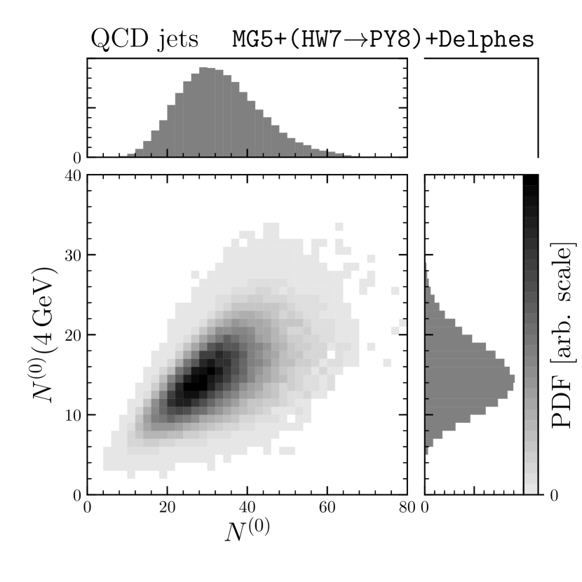
In section 5, we reweight the HW7 generated events to PY8 generated events by using $(N^{(0)},N^{(0)}(4\,\mathrm{GeV}))$ distribution. Since the two numbers are correlated as shown in figure 17, we transform the data first and calculate the reweighting factor using normalized histograms in order to ensure the efficiency of the reweighting. The transformation of $(N^{(0)},N^{(0)}(4\,\mathrm{GeV}))$ is defined as follows.

$$(x,y)\rightarrow(x^{\prime},y^{\prime})=(x,c_{1}-c_{2}y/x+c_{3}x),$$ (67)

where $c_{1}=3/2$, $c_{2}=2$, and $c_{3}=-1/60$. For each event, the reweighting factor in eq. (51) is calculated by the ratio of the corresponding bin values, $\rho_{\texttt{PY8}{}}/\rho_{\texttt{HW7}{}}$, where $\rho_{A}$ is the bin value of $(x^{\prime},y^{\prime})$ histogram with events generated by $A$. The reweighting factor for PY8 generated events to obtain distributions of HW7 generated events can be obtained by a similar procedure. The reweighted $(N^{(0)},N^{(0)}(4\,\mathrm{GeV}))$ distribution and $(N^{(0)},N^{(1)}/N^{(0)})$ distribution are shown in figure 24 and figure 25, respectively.

(a)

(b)

Figure 24: $(N^{(0)},N^{(0)}(4\,\mathrm{GeV}))$ distribution for (a) the weighted HW7 samples to reproduce PY8 distribution and (b) the weighted PY8 samples to reproduce HW7 distribution.

(a)

(b)

Figure 25: $N_{\mathrm{pixel}}$ vs $N_{1}/N_{\mathrm{pixel}}$ for (a) the weigthed HW7 sample to reproduce PY8 distribution and (b) the weighted PY8 sample. to reproduce HW7 distribution

References

- (1) A. J. Larkoski, I. Moult and B. Nachman, Jet Substructure at the Large Hadron Collider: A Review of Recent Advances in Theory and Machine Learning, Phys. Rept. 841 (2020) 1–63, [1709.04464].
- (2) R. Kogler et al., Jet Substructure at the Large Hadron Collider: Experimental Review, Rev. Mod. Phys. 91 (2019) 045003, [1803.06991].
- (3) D. Guest, K. Cranmer and D. Whiteson, Deep Learning and its Application to LHC Physics, Ann. Rev. Nucl. Part. Sci. 68 (2018) 161–181, [1806.11484].
- (4) A. Radovic, M. Williams, D. Rousseau, M. Kagan, D. Bonacorsi, A. Himmel et al., Machine learning at the energy and intensity frontiers of particle physics, Nature 560 (2018) 41–48.
- (5) M. Abdughani, J. Ren, L. Wu, J. M. Yang and J. Zhao, Supervised deep learning in high energy phenomenology: a mini review, Commun. Theor. Phys. 71 (2019) 955, [1905.06047].
- (6) L. G. Almeida, M. Backović, M. Cliche, S. J. Lee and M. Perelstein, Playing Tag with ANN: Boosted Top Identification with Pattern Recognition, JHEP 07 (2015) 086, [1501.05968].
- (7) L. de Oliveira, M. Kagan, L. Mackey, B. Nachman and A. Schwartzman, Jet-images — deep learning edition, JHEP 07 (2016) 069, [1511.05190].
- (8) P. T. Komiske, E. M. Metodiev and M. D. Schwartz, Deep learning in color: towards automated quark/gluon jet discrimination, JHEP 01 (2017) 110, [1612.01551].
- (9) A. Butter, G. Kasieczka, T. Plehn and M. Russell, Deep-learned Top Tagging with a Lorentz Layer, SciPost Phys. 5 (2018) 028, [1707.08966].
- (10) L. M. Dery, B. Nachman, F. Rubbo and A. Schwartzman, Weakly Supervised Classification in High Energy Physics, JHEP 05 (2017) 145, [1702.00414].
- (11) G. Kasieczka, T. Plehn, M. Russell and T. Schell, Deep-learning Top Taggers or The End of QCD?, JHEP 05 (2017) 006, [1701.08784].
- (12) G. Louppe, K. Cho, C. Becot and K. Cranmer, QCD-Aware Recursive Neural Networks for Jet Physics, JHEP 01 (2019) 057, [1702.00748].
- (13) T. Cheng, Recursive Neural Networks in Quark/Gluon Tagging, Comput. Softw. Big Sci. 2 (2018) 3, [1711.02633].
- (14) S. Egan, W. Fedorko, A. Lister, J. Pearkes and C. Gay, Long Short-Term Memory (LSTM) networks with jet constituents for boosted top tagging at the LHC, 1711.09059.
- (15) E. M. Metodiev, B. Nachman and J. Thaler, Classification without labels: Learning from mixed samples in high energy physics, JHEP 10 (2017) 174, [1708.02949].
- (16) P. T. Komiske, E. M. Metodiev and J. Thaler, Energy Flow Networks: Deep Sets for Particle Jets, JHEP 01 (2019) 121, [1810.05165].
- (17) S. Macaluso and D. Shih, Pulling Out All the Tops with Computer Vision and Deep Learning, JHEP 10 (2018) 121, [1803.00107].
- (18) A. Andreassen, I. Feige, C. Frye and M. D. Schwartz, JUNIPR: a Framework for Unsupervised Machine Learning in Particle Physics, Eur. Phys. J. C79 (2019) 102, [1804.09720].
- (19) S. H. Lim and M. M. Nojiri, Spectral Analysis of Jet Substructure with Neural Networks: Boosted Higgs Case, JHEP 10 (2018) 181, [1807.03312].
- (20) H. Qu and L. Gouskos, ParticleNet: Jet Tagging via Particle Clouds, Phys. Rev. D101 (2020) 056019, [1902.08570].
- (21) A. Chakraborty, S. H. Lim and M. M. Nojiri, Interpretable deep learning for two-prong jet classification with jet spectra, JHEP 07 (2019) 135, [1904.02092].
- (22) A. Andreassen, I. Feige, C. Frye and M. D. Schwartz, Binary JUNIPR: an interpretable probabilistic model for discrimination, Phys. Rev. Lett. 123 (2019) 182001, [1906.10137].
- (23) Y.-C. J. Chen, C.-W. Chiang, G. Cottin and D. Shih, Boosted and tagging with jet charge and deep learning, Phys. Rev. D101 (2020) 053001, [1908.08256].
- (24) T. Cheng, Interpretability Study on Deep Learning for Jet Physics at the Large Hadron Collider, in 33rd Annual Conference on Neural Information Processing Systems, 11, 2019. 1911.01872.
- (25) K.-F. Chen and Y.-T. Chien, Deep Learning Jet Substructure from Two-Particle Correlation, 1911.02020.
- (26) G. Kasieczka and D. Shih, DisCo Fever: Robust Networks Through Distance Correlation, 2001.05310.
- (27) T. Heimel, G. Kasieczka, T. Plehn and J. M. Thompson, QCD or What?, SciPost Phys. 6 (2019) 030, [1808.08979].
- (28) M. Farina, Y. Nakai and D. Shih, Searching for New Physics with Deep Autoencoders, Phys. Rev. D 101 (2020) 075021, [1808.08992].
- (29) J. Hajer, Y.-Y. Li, T. Liu and H. Wang, Novelty Detection Meets Collider Physics, Phys. Rev. D 101 (2020) 076015, [1807.10261].
- (30) B. M. Dillon, D. A. Faroughy and J. F. Kamenik, Uncovering latent jet substructure, Phys. Rev. D100 (2019) 056002, [1904.04200].
- (31) S. Diefenbacher, H. Frost, G. Kasieczka, T. Plehn and J. M. Thompson, CapsNets Continuing the Convolutional Quest, SciPost Phys. 8 (2020) 023, [1906.11265].
- (32) A. Blance, M. Spannowsky and P. Waite, Adversarially-trained autoencoders for robust unsupervised new physics searches, JHEP 10 (2019) 047, [1905.10384].
- (33) T. S. Roy and A. H. Vijay, A robust anomaly finder based on autoencoder, 1903.02032.
- (34) J. H. Collins, K. Howe and B. Nachman, Extending the search for new resonances with machine learning, Phys. Rev. D99 (2019) 014038, [1902.02634].
- (35) O. Amram and C. M. Suarez, Tag N’ Train: A Technique to Train Improved Classifiers on Unlabeled Data, 2002.12376.
- (36) B. Nachman and D. Shih, Anomaly Detection with Density Estimation, Phys. Rev. D 101 (2020) 075042, [2001.04990].
- (37) A. Andreassen, B. Nachman and D. Shih, Simulation Assisted Likelihood-free Anomaly Detection, Phys. Rev. D 101 (2020) 095004, [2001.05001].
- (38) D. Guest, J. Collado, P. Baldi, S.-C. Hsu, G. Urban and D. Whiteson, Jet Flavor Classification in High-Energy Physics with Deep Neural Networks, Phys. Rev. D94 (2016) 112002, [1607.08633].
- (39) ATLAS collaboration, Identification of Jets Containing -Hadrons with Recurrent Neural Networks at the ATLAS Experiment, Tech. Rep. ATL-PHYS-PUB-2017-003, CERN, Geneva, Mar, 2017.
- (40) CMS collaboration, Heavy flavor identification at CMS with deep neural networks, Tech. Rep. CMS-DP-2017-005, Mar, 2017.
- (41) J. Arjona Martínez, O. Cerri, M. Pierini, M. Spiropulu and J.-R. Vlimant, Pileup mitigation at the Large Hadron Collider with graph neural networks, Eur. Phys. J. Plus 134 (2019) 333, [1810.07988].
- (42) P. T. Komiske, E. M. Metodiev, B. Nachman and M. D. Schwartz, Pileup Mitigation with Machine Learning (PUMML), JHEP 12 (2017) 051, [1707.08600].
- (43) P. T. Komiske, E. M. Metodiev, B. Nachman and M. D. Schwartz, Learning to Remove Pileup at the LHC with Jet Images, J. Phys. Conf. Ser. 1085 (2018) 042010.
- (44) J. Bendavid, Efficient Monte Carlo Integration Using Boosted Decision Trees and Generative Deep Neural Networks, 1707.00028.
- (45) M. D. Klimek and M. Perelstein, Neural Network-Based Approach to Phase Space Integration, 1810.11509.
- (46) S. Otten, S. Caron, W. de Swart, M. van Beekveld, L. Hendriks, C. van Leeuwen et al., Event Generation and Statistical Sampling for Physics with Deep Generative Models and a Density Information Buffer, 1901.00875.
- (47) B. Hashemi, N. Amin, K. Datta, D. Olivito and M. Pierini, LHC analysis-specific datasets with Generative Adversarial Networks, 1901.05282.
- (48) R. Di Sipio, M. Faucci Giannelli, S. Ketabchi Haghighat and S. Palazzo, DijetGAN: A Generative-Adversarial Network Approach for the Simulation of QCD Dijet Events at the LHC, JHEP 08 (2020) 110, [1903.02433].
- (49) A. Butter, T. Plehn and R. Winterhalder, How to GAN LHC Events, SciPost Phys. 7 (2019) 075, [1907.03764].
- (50) S. Carrazza and F. A. Dreyer, Lund jet images from generative and cycle-consistent adversarial networks, Eur. Phys. J. C79 (2019) 979, [1909.01359].
- (51) SHiP collaboration, C. Ahdida et al., Fast simulation of muons produced at the SHiP experiment using Generative Adversarial Networks, JINST 14 (2019) P11028, [1909.04451].
- (52) A. Butter, T. Plehn and R. Winterhalder, How to GAN Event Subtraction, 1912.08824.
- (53) F. Bishara and M. Montull, (Machine) Learning Amplitudes for Faster Event Generation, 1912.11055.
- (54) E. Bothmann, T. Janßen, M. Knobbe, T. Schmale and S. Schumann, Exploring phase space with Neural Importance Sampling, SciPost Phys. 8 (2020) 069, [2001.05478].
- (55) C. Gao, J. Isaacson and C. Krause, i-flow: High-Dimensional Integration and Sampling with Normalizing Flows, 2001.05486.
- (56) C. Gao, S. Höche, J. Isaacson, C. Krause and H. Schulz, Event Generation with Normalizing Flows, Phys. Rev. D 101 (2020) 076002, [2001.10028].
- (57) K. T. Matchev and P. Shyamsundar, Uncertainties associated with GAN-generated datasets in high energy physics, 2002.06307.
- (58) S. Badger and J. Bullock, Using neural networks for efficient evaluation of high multiplicity scattering amplitudes, 2002.07516.
- (59) A. Andreassen, P. T. Komiske, E. M. Metodiev, B. Nachman and J. Thaler, OmniFold: A Method to Simultaneously Unfold All Observables, Phys. Rev. Lett. 124 (2020) 182001, [1911.09107].
- (60) M. Bellagente, A. Butter, G. Kasieczka, T. Plehn and R. Winterhalder, How to GAN away Detector Effects, SciPost Phys. 8 (2020) 070, [1912.00477].
- (61) S. Forte, L. Garrido, J. I. Latorre and A. Piccione, Neural network parametrization of deep inelastic structure functions, JHEP 05 (2002) 062, [hep-ph/0204232].
- (62) S. Forte, J. I. Latorre, L. Magnea and A. Piccione, Determination of alpha(s) from scaling violations of truncated moments of structure functions, Nucl. Phys. B643 (2002) 477–500, [hep-ph/0205286].
- (63) J. Rojo and J. I. Latorre, Neural network parametrization of spectral functions from hadronic tau decays and determination of QCD vacuum condensates, JHEP 01 (2004) 055, [hep-ph/0401047].
- (64) NNPDF collaboration, L. Del Debbio, S. Forte, J. I. Latorre, A. Piccione and J. Rojo, Unbiased determination of the proton structure function F(2)**p with faithful uncertainty estimation, JHEP 03 (2005) 080, [hep-ph/0501067].
- (65) NNPDF collaboration, L. Del Debbio, S. Forte, J. I. Latorre, A. Piccione and J. Rojo, Neural network determination of parton distributions: The Nonsinglet case, JHEP 03 (2007) 039, [hep-ph/0701127].
- (66) NNPDF collaboration, R. D. Ball, L. Del Debbio, S. Forte, A. Guffanti, J. I. Latorre, A. Piccione et al., A Determination of parton distributions with faithful uncertainty estimation, Nucl. Phys. B809 (2009) 1–63, [0808.1231].
- (67) NNPDF collaboration, R. D. Ball, L. Del Debbio, S. Forte, A. Guffanti, J. I. Latorre, A. Piccione et al., Precision determination of electroweak parameters and the strange content of the proton from neutrino deep-inelastic scattering, Nucl. Phys. B823 (2009) 195–233, [0906.1958].
- (68) R. D. Ball, L. Del Debbio, S. Forte, A. Guffanti, J. I. Latorre, J. Rojo et al., A first unbiased global NLO determination of parton distributions and their uncertainties, Nucl. Phys. B838 (2010) 136–206, [1002.4407].
- (69) NNPDF collaboration, R. D. Ball, V. Bertone, F. Cerutti, L. Del Debbio, S. Forte, A. Guffanti et al., Reweighting NNPDFs: the W lepton asymmetry, Nucl. Phys. B 849 (2011) 112–143, [1012.0836].
- (70) R. D. Ball, V. Bertone, F. Cerutti, L. Del Debbio, S. Forte, A. Guffanti et al., Impact of Heavy Quark Masses on Parton Distributions and LHC Phenomenology, Nucl. Phys. B849 (2011) 296–363, [1101.1300].
- (71) S. Lionetti, R. D. Ball, V. Bertone, F. Cerutti, L. Del Debbio, S. Forte et al., Precision determination of using an unbiased global NLO parton set, Phys. Lett. B701 (2011) 346–352, [1103.2369].
- (72) R. D. Ball et al., Parton distributions with LHC data, Nucl. Phys. B867 (2013) 244–289, [1207.1303].
- (73) NNPDF collaboration, R. D. Ball, V. Bertone, S. Carrazza, L. Del Debbio, S. Forte, A. Guffanti et al., Parton distributions with QED corrections, Nucl. Phys. B877 (2013) 290–320, [1308.0598].
- (74) NNPDF collaboration, S. Carrazza, Towards the determination of the photon parton distribution function constrained by LHC data, PoS DIS2013 (2013) 279, [1307.1131].
- (75) NNPDF collaboration, S. Carrazza, Towards an unbiased determination of parton distributions with QED corrections, in Proceedings, 48th Rencontres de Moriond on QCD and High Energy Interactions: La Thuile, Italy, March 9-16, 2013, pp. 357–360, 2013. 1305.4179.
- (76) NNPDF collaboration, R. D. Ball et al., Parton distributions for the LHC Run II, JHEP 04 (2015) 040, [1410.8849].
- (77) NNPDF collaboration, R. D. Ball et al., Parton distributions from high-precision collider data, Eur. Phys. J. C77 (2017) 663, [1706.00428].
- (78) NNPDF collaboration, V. Bertone, S. Carrazza, N. P. Hartland, E. R. Nocera and J. Rojo, A determination of the fragmentation functions of pions, kaons, and protons with faithful uncertainties, Eur. Phys. J. C77 (2017) 516, [1706.07049].
- (79) A. Butter et al., The Machine Learning Landscape of Top Taggers, SciPost Phys. 7 (2019) 014, [1902.09914].
- (80) ATLAS collaboration, M. Aaboud et al., Performance of top-quark and -boson tagging with ATLAS in Run 2 of the LHC, Eur. Phys. J. C79 (2019) 375, [1808.07858].
- (81) J. M. Butterworth, A. R. Davison, M. Rubin and G. P. Salam, Jet substructure as a new Higgs search channel at the LHC, Phys. Rev. Lett. 100 (2008) 242001, [0802.2470].
- (82) J. Thaler and L.-T. Wang, Strategies to Identify Boosted Tops, JHEP 07 (2008) 092, [0806.0023].
- (83) D. E. Kaplan, K. Rehermann, M. D. Schwartz and B. Tweedie, Top Tagging: A Method for Identifying Boosted Hadronically Decaying Top Quarks, Phys. Rev. Lett. 101 (2008) 142001, [0806.0848].
- (84) S. D. Ellis, C. K. Vermilion and J. R. Walsh, Techniques for improved heavy particle searches with jet substructure, Phys. Rev. D80 (2009) 051501, [0903.5081].
- (85) CMS collaboration, A Cambridge-Aachen (C-A) based Jet Algorithm for boosted top-jet tagging, Tech. Rep. CMS-PAS-JME-09-001, CERN, 2009. Geneva, Jul, 2009.
- (86) T. Plehn, G. P. Salam and M. Spannowsky, Fat Jets for a Light Higgs, Phys. Rev. Lett. 104 (2010) 111801, [0910.5472].
- (87) T. Plehn, M. Spannowsky, M. Takeuchi and D. Zerwas, Stop Reconstruction with Tagged Tops, JHEP 10 (2010) 078, [1006.2833].
- (88) M. Dasgupta, A. Fregoso, S. Marzani and G. P. Salam, Towards an understanding of jet substructure, JHEP 09 (2013) 029, [1307.0007].
- (89) A. J. Larkoski, S. Marzani, G. Soyez and J. Thaler, Soft Drop, JHEP 05 (2014) 146, [1402.2657].
- (90) D. Krohn, J. Thaler and L.-T. Wang, Jet Trimming, JHEP 02 (2010) 084, [0912.1342].
- (91) D. E. Soper and M. Spannowsky, Finding physics signals with shower deconstruction, Phys. Rev. D84 (2011) 074002, [1102.3480].
- (92) D. E. Soper and M. Spannowsky, Finding top quarks with shower deconstruction, Phys. Rev. D87 (2013) 054012, [1211.3140].
- (93) D. E. Soper and M. Spannowsky, Finding physics signals with event deconstruction, Phys. Rev. D89 (2014) 094005, [1402.1189].
- (94) F. V. Tkachov, Measuring multi - jet structure of hadronic energy flow or What is a jet?, Int. J. Mod. Phys. A12 (1997) 5411–5529, [hep-ph/9601308].
- (95) J. Thaler and K. Van Tilburg, Identifying Boosted Objects with N-subjettiness, JHEP 03 (2011) 015, [1011.2268].
- (96) M. Jankowiak and A. J. Larkoski, Jet Substructure Without Trees, JHEP 06 (2011) 057, [1104.1646].
- (97) M. Jankowiak and A. J. Larkoski, Angular Scaling in Jets, JHEP 04 (2012) 039, [1201.2688].
- (98) A. J. Larkoski, QCD Analysis of the Scale-Invariance of Jets, Phys. Rev. D86 (2012) 054004, [1207.1437].
- (99) J. Gallicchio and M. D. Schwartz, Quark and Gluon Jet Substructure, JHEP 04 (2013) 090, [1211.7038].
- (100) A. J. Larkoski, G. P. Salam and J. Thaler, Energy Correlation Functions for Jet Substructure, JHEP 06 (2013) 108, [1305.0007].
- (101) A. J. Larkoski, I. Moult and D. Neill, Power Counting to Better Jet Observables, JHEP 12 (2014) 009, [1409.6298].
- (102) I. Moult, L. Necib and J. Thaler, New Angles on Energy Correlation Functions, JHEP 12 (2016) 153, [1609.07483].
- (103) P. T. Komiske, E. M. Metodiev and J. Thaler, Energy flow polynomials: A complete linear basis for jet substructure, JHEP 04 (2018) 013, [1712.07124].
- (104) H. Chen, M.-X. Luo, I. Moult, T.-Z. Yang, X. Zhang and H. X. Zhu, Three Point Energy Correlators in the Collinear Limit: Symmetries, Dualities and Analytic Results, 1912.11050.
- (105) C. Frye, A. J. Larkoski, J. Thaler and K. Zhou, Casimir Meets Poisson: Improved Quark/Gluon Discrimination with Counting Observables, JHEP 09 (2017) 083, [1704.06266].
- (106) J. Gallicchio and M. D. Schwartz, Seeing in Color: Jet Superstructure, Phys. Rev. Lett. 105 (2010) 022001, [1001.5027].
- (107) J. Gallicchio, J. Huth, M. Kagan, M. D. Schwartz, K. Black and B. Tweedie, Multivariate discrimination and the Higgs + W/Z search, JHEP 04 (2011) 069, [1010.3698].
- (108) A. Hook, M. Jankowiak and J. G. Wacker, Jet Dipolarity: Top Tagging with Color Flow, JHEP 04 (2012) 007, [1102.1012].
- (109) S. Choi, S. J. Lee and M. Perelstein, Infrared Safety of a Neural-Net Top Tagging Algorithm, JHEP 02 (2019) 132, [1806.01263].
- (110) S. Bollweg, M. Haußmann, G. Kasieczka, M. Luchmann, T. Plehn and J. Thompson, Deep-Learning Jets with Uncertainties and More, SciPost Phys. 8 (2020) 006, [1904.10004].
- (111) G. Kasieczka, M. Luchmann, F. Otterpohl and T. Plehn, Per-Object Systematics using Deep-Learned Calibration, 2003.11099.
- (112) M. Gori, G. Monfardini and F. Scarselli, A new model for learning in graph domains, in Proceedings. 2005 IEEE International Joint Conference on Neural Networks, 2005., vol. 2, pp. 729–734 vol. 2, July, 2005. DOI.
- (113) F. Scarselli, M. Gori, A. C. Tsoi, M. Hagenbuchner and G. Monfardini, The graph neural network model, IEEE Transactions on Neural Networks 20 (Jan, 2009) 61–80.
- (114) D. Raposo, A. Santoro, D. G. T. Barrett, R. Pascanu, T. P. Lillicrap and P. W. Battaglia, Discovering objects and their relations from entangled scene representations, CoRR abs/1702.05068 (2017) , [1702.05068].
- (115) A. Santoro, D. Raposo, D. G. Barrett, M. Malinowski, R. Pascanu, P. Battaglia et al., A simple neural network module for relational reasoning, in Advances in Neural Information Processing Systems 30 (I. Guyon, U. V. Luxburg, S. Bengio, H. Wallach, R. Fergus, S. Vishwanathan et al., eds.), pp. 4967–4976. Curran Associates, Inc., 2017.
- (116) P. W. Battaglia, J. B. Hamrick, V. Bapst, A. Sanchez-Gonzalez, V. F. Zambaldi, M. Malinowski et al., Relational inductive biases, deep learning, and graph networks, CoRR abs/1806.01261 (2018) , [1806.01261].
- (117) I. Henrion, J. Brehmer, J. Bruna, K. Cho, K. Cranmer, G. Louppe et al., Neural message passing for jet physics, in Proceedings of the Deep Learning for Physical Sciences (DLPS) 2017 workshop at the 31st Annual Conference on Neural Information Processing Systems (NeurlIPS), 2017.
- (118) S. R. Qasim, J. Kieseler, Y. Iiyama and M. Pierini, Learning representations of irregular particle-detector geometry with distance-weighted graph networks, Eur. Phys. J. C79 (2019) 608, [1902.07987].
- (119) M. Abdughani, J. Ren, L. Wu and J. M. Yang, Probing stop pair production at the LHC with graph neural networks, JHEP 08 (2019) 055, [1807.09088].
- (120) E. A. Moreno, O. Cerri, J. M. Duarte, H. B. Newman, T. Q. Nguyen, A. Periwal et al., JEDI-net: a jet identification algorithm based on interaction networks, Eur. Phys. J. C80 (2020) 58, [1908.05318].
- (121) E. A. Moreno, T. Q. Nguyen, J.-R. Vlimant, O. Cerri, H. B. Newman, A. Periwal et al., Interaction networks for the identification of boosted decays, 1909.12285.
- (122) J. Ren, L. Wu and J. M. Yang, Unveiling CP property of top-Higgs coupling with graph neural networks at the LHC, Phys. Lett. B802 (2020) 135198, [1901.05627].
- (123) V. Mikuni and F. Canelli, ABCNet: An attention-based method for particle tagging, 2001.05311.
- (124) T. Bister, M. Erdmann, J. Glombitza, N. Langner, J. Schulte and M. Wirtz, Identification of Patterns in Cosmic-Ray Arrival Directions using Dynamic Graph Convolutional Neural Networks, 2003.13038.
- (125) C. L. Basham, L. S. Brown, S. D. Ellis and S. T. Love, Energy Correlations in electron - Positron Annihilation: Testing QCD, Phys. Rev. Lett. 41 (1978) 1585.
- (126) C. L. Basham, L. S. Brown, S. D. Ellis and S. T. Love, Energy Correlations in electron-Positron Annihilation in Quantum Chromodynamics: Asymptotically Free Perturbation Theory, Phys. Rev. D19 (1979) 2018.
- (127) C. L. Basham and S. T. Love, Energy Correlations in Electron - Positron Annihilation: Sensitivity of Quantum Chromodynamics Tests to Gluon Spin, Phys. Rev. D20 (1979) 340.
- (128) C. L. Basham, L. S. Brown, S. D. Ellis and S. T. Love, Energy Correlations in Perturbative Quantum Chromodynamics: A Conjecture for All Orders, Phys. Lett. 85B (1979) 297–299.
- (129) K. R. Mecke, T. Buchert and H. Wagner, Robust morphological measures for large scale structure in the universe, Astron. Astrophys. 288 (1994) 697–704, [astro-ph/9312028].
- (130) J. Schmalzing, M. Kerscher and T. Buchert, Minkowski functionals in cosmology, Proc. Int. Sch. Phys. Fermi 132 (1996) 281–291, [astro-ph/9508154].
- (131) J. Schmalzing and T. Buchert, Beyond genus statistics: A Unifying approach to the morphology of cosmic structure, Astrophys. J. 482 (1997) L1–L4, [astro-ph/9702130].
- (132) J. Schmalzing and K. M. Gorski, Minkowski functionals used in the morphological analysis of cosmic microwave background anisotropy maps, Mon. Not. Roy. Astron. Soc. 297 (1998) 355, [astro-ph/9710185].
- (133) S. Winitzki and A. Kosowsky, Minkowski functional description of microwave background gaussianity, New Astronomy 3 (1998) 75 – 99.
- (134) M. Kerscher, K. Mecke, P. Schuecker, H. Bohringer, L. Guzzo, C. A. Collins et al., Non-gaussian morphology on large scales: Minkowski functionals of the reflex cluster catalogue, Astron. Astrophys. 377 (2001) 1, [astro-ph/0105150].
- (135) C. Beisbart, T. Buchert and H. Wagner, Morphometry of spatial patterns, Physica A293 (2001) 592–604, [astro-ph/0007459].
- (136) T. Matsubara, Statistics of smoothed cosmic fields in perturbation theory. i. formulation and useful formulae in second-order perturbation theory, The Astrophysical Journal 584 (feb, 2003) 1–33, [astro-ph/0006269].
- (137) C. Hikage, E. Komatsu and T. Matsubara, Primordial Non-Gaussianity and Analytical Formula for Minkowski Functionals of the Cosmic Microwave Background and Large-scale Structure, Astrophys. J. 653 (2006) 11–26, [astro-ph/0607284].
- (138) D. Göring, M. A. Klatt, C. Stegmann and K. Mecke, Morphometric analysis in gamma-ray astronomy using Minkowski functionals, Astronomy & Astrophysics 555 (Jun, 2013) A38.
- (139) M. A. Klatt and K. Mecke, Morphometric analysis in gamma-ray astronomy using Minkowski functionals: II. Joint structure quantification, 1710.03542.
- (140) M. A. Klatt and K. Mecke, Morphometric analysis in gamma-ray astronomy using Minkowski functionals: III. Sensitivity increase via a refined structure quantification, 1710.03543.
- (141) P. Chingangbam, V. Ganesan, K. P. Yogendran and C. Park, On Minkowski Functionals of CMB polarization, Phys. Lett. B771 (2017) 67–73, [1705.04454].
- (142) P. Pranav, R. van de Weygaert, G. Vegter, B. J. T. Jones, R. J. Adler, J. Feldbrugge et al., Topology and Geometry of Gaussian random fields I: on Betti Numbers, Euler characteristic and Minkowski functionals, Mon. Not. Roy. Astron. Soc. 485 (2019) 4167–4208, [1812.07310].
- (143) K. R. Mecke, Morphological characterization of patterns in reaction-diffusion systems, Phys. Rev. E 53 (May, 1996) 4794–4800.
- (144) K. R. Mecke, Additivity, convexity, and beyond: Applications of minkowski functionals in statistical physics, in Statistical Physics and Spatial Statistics (K. R. Mecke and D. Stoyan, eds.), (Berlin, Heidelberg), pp. 111–184, Springer Berlin Heidelberg, 2000.
- (145) H. Mantz, K. Jacobs and K. Mecke, Utilizing minkowski functionals for image analysis: a marching square algorithm, Journal of Statistical Mechanics: Theory and Experiment 2008 (dec, 2008) P12015.
- (146) J. Lin, M. Freytsis, I. Moult and B. Nachman, Boosting with Machine Learning, JHEP 10 (2018) 101, [1807.10768].
- (147) Y.-T. Chien, Telescoping jets: Probing hadronic event structure with multiple R ’s, Phys. Rev. D90 (2014) 054008, [1304.5240].
- (148) Y.-T. Chien, A. Emerman, S.-C. Hsu, S. Meehan and Z. Montague, Telescoping jet substructure, 1711.11041.
- (149) H. Hadwigeb, Integralsätze im konvexring, Abhandlungen aus dem Mathematischen Seminar der Universität Hamburg 20 (1956) 136–154.
- (150) A. Cole and G. Shiu, Persistent Homology and Non-Gaussianity, JCAP 1803 (2018) 025, [1712.08159].
- (151) A. Cole and G. Shiu, Topological Data Analysis for the String Landscape, JHEP 03 (2019) 054, [1812.06960].
- (152) J. Alwall, R. Frederix, S. Frixione, V. Hirschi, F. Maltoni, O. Mattelaer et al., The automated computation of tree-level and next-to-leading order differential cross sections, and their matching to parton shower simulations, JHEP 07 (2014) 079, [1405.0301].
- (153) T. Sjöstrand, S. Ask, J. R. Christiansen, R. Corke, N. Desai, P. Ilten et al., An Introduction to PYTHIA 8.2, Comput. Phys. Commun. 191 (2015) 159–177, [1410.3012].
- (154) J. Bellm et al., Herwig 7.0/Herwig++ 3.0 release note, Eur. Phys. J. C76 (2016) 196, [1512.01178].
- (155) M. Bahr et al., Herwig++ Physics and Manual, Eur. Phys. J. C58 (2008) 639–707, [0803.0883].
- (156) DELPHES 3 collaboration, J. de Favereau, C. Delaere, P. Demin, A. Giammanco, V. Lemaître, A. Mertens et al., DELPHES 3, A modular framework for fast simulation of a generic collider experiment, JHEP 02 (2014) 057, [1307.6346].
- (157) D. Clevert, T. Unterthiner and S. Hochreiter, Fast and Accurate Deep Network Learning by Exponential Linear Units (ELUs), in The International Conference on Learning Representations (ICLR), 2016. 1511.07289.
- (158) S. J. Hanson and L. Y. Pratt, Comparing biases for minimal network construction with back-propagation, in Advances in Neural Information Processing Systems 1 (D. S. Touretzky, ed.), pp. 177–185. Morgan-Kaufmann, 1989.
- (159) A. S. Weigend, D. E. Rumelhart and B. A. Huberman, Generalization by weight-elimination with application to forecasting, in Advances in Neural Information Processing Systems 3 (R. P. Lippmann, J. E. Moody and D. S. Touretzky, eds.), pp. 875–882. Morgan-Kaufmann, 1991.
- (160) A. Krogh and J. A. Hertz, A simple weight decay can improve generalization, in Advances in Neural Information Processing Systems 4 (J. E. Moody, S. J. Hanson and R. P. Lippmann, eds.), pp. 950–957. Morgan-Kaufmann, 1992.
- (161) D. P. Kingma and J. Ba, Adam: A method for stochastic optimization, in The 3rd International Conference for Learning Representations, 2014. 1412.6980.
- (162) K. He, X. Zhang, S. Ren and J. Sun, Delving deep into rectifiers: Surpassing human-level performance on imagenet classification, in The IEEE International Conference on Computer Vision (ICCV), December, 2015. 1502.01852.
- (163) F. Chollet et al., “Keras.” https://keras.io, 2015.
- (164) M. Abadi, A. Agarwal, P. Barham, E. Brevdo, Z. Chen, C. Citro et al., “TensorFlow: Large-scale machine learning on heterogeneous systems.” https://www.tensorflow.org/, 2015.
- (165) F. A. Dreyer, L. Necib, G. Soyez and J. Thaler, Recursive Soft Drop, JHEP 06 (2018) 093, [1804.03657].
- (166) Y. Wang, Y. Sun, Z. Liu, S. E. Sarma, M. M. Bronstein and J. M. Solomon, Dynamic graph cnn for learning on point clouds, ACM Trans. Graph. 38 (Oct., 2019) , [1801.07829].
- (167) S. Xie, R. Girshick, P. Dollar, Z. Tu and K. He, Aggregated residual transformations for deep neural networks, in The IEEE Conference on Computer Vision and Pattern Recognition (CVPR), July, 2017. 1611.05431.
- (168) K. He, X. Zhang, S. Ren and J. Sun, Deep residual learning for image recognition, in 2016 IEEE Conference on Computer Vision and Pattern Recognition (CVPR), pp. 770–778, June, 2016. 1512.03385. DOI.
- (169) S. Gieseke, P. Stephens and B. Webber, New formalism for QCD parton showers, JHEP 12 (2003) 045, [hep-ph/0310083].
- (170) B. R. Webber, A QCD Model for Jet Fragmentation Including Soft Gluon Interference, Nucl. Phys. B238 (1984) 492–528.
- (171) T. Sjostrand and P. Z. Skands, Transverse-momentum-ordered showers and interleaved multiple interactions, Eur. Phys. J. C39 (2005) 129–154, [hep-ph/0408302].
- (172) B. Andersson, G. Gustafson, G. Ingelman and T. Sjostrand, Parton Fragmentation and String Dynamics, Phys. Rept. 97 (1983) 31–145.
- (173) T. Sjostrand, Jet Fragmentation of Nearby Partons, Nucl. Phys. B248 (1984) 469–502.
- (174) A. J. Larkoski, J. Thaler and W. J. Waalewijn, Gaining (Mutual) Information about Quark/Gluon Discrimination, JHEP 11 (2014) 129, [1408.3122].
- (175) P. Gras, S. Höche, D. Kar, A. Larkoski, L. Lönnblad, S. Plätzer et al., Systematics of quark/gluon tagging, JHEP 07 (2017) 091, [1704.03878].
- (176) A. Andreassen and B. Nachman, Neural Networks for Full Phase-space Reweighting and Parameter Tuning, 1907.08209.
- (177) P. Skands, S. Carrazza and J. Rojo, Tuning PYTHIA 8.1: the Monash 2013 Tune, Eur. Phys. J. C74 (2014) 3024, [1404.5630].
- (178) J. Bellm et al., “Minimum-bias and underlying-event tunes.” https://herwig.hepforge.org/tutorials/mpi/tunes.html, 2015.
- (179) S. Gieseke, C. Rohr and A. Siodmok, Colour reconnections in Herwig++, Eur. Phys. J. C72 (2012) 2225, [1206.0041].
- (180) M. Cacciari, G. P. Salam and G. Soyez, The Anti-k(t) jet clustering algorithm, JHEP 04 (2008) 063, [0802.1189].
- (181) M. Cacciari, G. P. Salam and G. Soyez, FastJet User Manual, Eur. Phys. J. C72 (2012) 1896, [1111.6097].
- (182) M. Cacciari and G. P. Salam, Dispelling the myth for the jet-finder, Phys. Lett. B641 (2006) 57–61, [hep-ph/0512210].
- (183) S. Catani, Y. L. Dokshitzer, M. H. Seymour and B. R. Webber, Longitudinally invariant clustering algorithms for hadron hadron collisions, Nucl. Phys. B406 (1993) 187–224.
- (184) S. D. Ellis and D. E. Soper, Successive combination jet algorithm for hadron collisions, Phys. Rev. D48 (1993) 3160–3166, [hep-ph/9305266].