1

Nonconvex Sparse Regularization for Deep Neural Networks and its Optimality

Ilsang Ohn^1
1Department of Applied and Computational Mathematics and Statistics, University of Notre Dame, Notre Dame, IN 46556, USA
Yongdai Kim^2
2Department of Statistics, Seoul National University, Seoul 08826, Republic of Korea

Abstract

Recent theoretical studies proved that deep neural network (DNN) estimators obtained by minimizing empirical risk with a certain sparsity constraint can attain optimal convergence rates for regression and classification problems. However, the sparsity constraint requires to know certain properties of the true model, which are not available in practice. Moreover, computation is difficult due to the discrete nature of the sparsity constraint. In this paper, we propose a novel penalized estimation method for sparse DNNs, which resolves the aforementioned problems existing in the sparsity constraint. We establish an oracle inequality for the excess risk of the proposed sparse-penalized DNN estimator and derive convergence rates for several learning tasks. In particular, we prove that the sparse-penalized estimator can adaptively attain minimax convergence rates for various nonparametric regression problems. For computation, we develop an efficient gradient-based optimization algorithm that guarantees the monotonic reduction of the objective function.

Keywords: Deep neural network, Adaptiveness, Penalization, Minimax optimality, Sparsity

1 Introduction

Sparse learning of deep neural networks (DNN) has received much attention in artificial intelligence and statistics. In artificial intelligence, there are a lot of evidences (Han et al., 2015; Frankle and Carbin, 2018; Louizos et al., 2018) to support that sparse DNN can reduce the complexity of a leaned DNN significantly (in terms of the number of parameters as well as the numbers of hidden layers and hidden nodes) without hampering prediction accuracy much. By doing so, we can reduce memory and energy consumption at the prediction phase.

In statistics, recent studies about DNNs for nonparametric regression and classification (Schmidt-Hieber, 2020; Imaizumi and Fukumizu, 2019; Suzuki, 2019; Bauer and Kohler, 2019; Kim et al., 2021) proved that a DNN estimator minimizing an empirical risk with a certain sparsity constraint achieves the minimax optimality for a wide class of functions including smooth functions, piecewise smooth functions and smooth decision boundaries. However, there are still two unanswered questions. The first question is how to choose a suitable level of sparsity, which depends on the unknown smoothness and/or the unknown intrinsic dimensionality of the true function. The second question is computation. Learning a deep architecture with a given sparsity constraint is computationally intractable since we need to explore a large number of possible configurations of sparsity pattern in the network parameter.

More recently, Kohler and Langer (2021) showed that the empirical risk minimizer over fully connected (i.e., non-sparse) DNNs can have minimax optimality also. Although removing the sparse constraint circumvents the related computation issue, their result is still nonadaptive because the appropriate number of hidden nodes should depend on the unknown smoothness of the true regression function.

In this paper, we propose a novel learning method of sparse DNNs for nonparametric regression and classification, which answers the aforementioned two questions in the sparsity-constrained empirical risk minimization (ERM) method. The proposed learning algorithm is to learn a DNN by minimizing the penalized empirical risk, which is the sum of the empirical risk and the clipped $L_{1}$ penalty (Zhang, 2010b). By choosing the position of the clipping in the clipped $L_{1}$ penalty carefully, we establish an oracle inequality for the excess risk of the proposed sparse DNN estimator and derive convergence rates for several learning tasks. In particular, it will be shown that the proposed DNN estimator can adaptively attain minimax convergence rates for various nonparametric regression problems.

Although nonconvex penalties such as the clipped $L_{1}$ penalty are popular for high-dimensional linear regressions (Fan and Li, 2001; Zhang, 2010a), they are not popularly used for DNN. Instead, $L_{1}$ norm-based penalties such as Lasso and Group Lasso are popular (Liu et al., 2015; Wen et al., 2016). This would be partly because of the convexity of the $L_{1}$ penalty. For computation with the clipped $L_{1}$ penalty, we develop an mini-batch optimization algorithm by combining the proximal gradient descent algorithm (Parikh et al., 2014) and the concave-convex procedure (CCCP) (Yuille and Rangarajan, 2003). The CCCP is a procedure to replace the clipped $L_{1}$ penalty by its tight convex upper bound to make the optimization problem be $L_{1}$ penalized, and the proximal gradient descent algorithm is a mini-batch optimization algorithm for $L_{1}$ penalized optimization problems.

1.1 Notation

We denote by $\mathbbm{1}(\cdot)$ the indicator function. Let $\mathbb{R}$ be the set of real numbers and $\mathbbm{N}$ be the set of natural numbers. Let $\mathbbm{N}_{0}\mathrel{\mathop{\ordinarycolon}}=\mathbbm{N}\cup\{0\}.$ Let $[m]\mathrel{\mathop{\ordinarycolon}}=\{1,2,\dots,m\}$ for $m\in\mathbbm{N}$. For two real numbers $a$ and $b$, we write $a\vee b\mathrel{\mathop{\ordinarycolon}}=\max\{a,b\}$ and $a\wedge b\mathrel{\mathop{\ordinarycolon}}=\min\{a,b\}$. For a real valued vector $\mathbf{x}\equiv(x_{1},\dots,x_{d})\in\mathbb{R}^{d}$, we let $\mathinner{\!\left\lVert\mathbf{x}\right\rVert}_{0}\mathrel{\mathop{\ordinarycolon}}=\sum_{j=1}^{d}\mathbbm{1}(x_{j}\neq 0)$, $\mathinner{\!\left\lVert\mathbf{x}\right\rVert}_{p}\mathrel{\mathop{\ordinarycolon}}=\mathinner{\left(\sum_{j=1}^{d}|x_{j}|^{p}\right)}^{1/p}$ for $p\in[1,\infty)$ and $\mathinner{\!\left\lVert\mathbf{x}\right\rVert}_{\infty}\mathrel{\mathop{\ordinarycolon}}=\max_{1\leq j\leq d}|x_{j}|$. For a real-valued function $f\mathrel{\mathop{\ordinarycolon}}\mathcal{X}\mapsto\mathbb{R}$, we let $\mathinner{\!\left\lVert f\right\rVert}_{\infty,\mathcal{X}}\mathrel{\mathop{\ordinarycolon}}=\sup_{\mathbf{x}\in\mathcal{X}}|f(\mathbf{x})|.$ If the domain of the function $f$ is clear in the context, we omit the subscript $\mathcal{X}$ to write $\mathinner{\!\left\lVert f\right\rVert}_{\infty}\mathrel{\mathop{\ordinarycolon}}=\mathinner{\!\left\lVert f\right\rVert}_{\infty,\mathcal{X}}$. For $p\in[1,\infty)$ and a distribution $\mathsf{Q}$ on $\mathcal{X}$, let $\|f\|_{p,Q}\mathrel{\mathop{\ordinarycolon}}=\mathinner{\left(\int|f(\mathbf{x})|^{p}\mathrm{d}\mathsf{Q}(\mathbf{x})\right)}^{1/p}$. For two positive sequences $\{a_{n}\}_{n\in\mathbb{N}}$ and $\{b_{n}\}_{n\in\mathbb{N}}$, we write $a_{n}\lesssim b_{n}$ or $b_{n}\gtrsim a_{n}$ if there exists a positive constant $C>0$ such that $a_{n}\leq Cb_{n}$ for any $n\in\mathbb{N}$. We also write $a_{n}\asymp b_{n}$ if $a_{n}\lesssim b_{n}$ and $a_{n}\gtrsim b_{n}$.

1.2 Deep neural networks

A DNN with $L\in\mathbbm{N}$ layers, $N_{l}\in\mathbbm{N}$ many nodes at the $l$-th hidden layer for $l=[L]$, input of dimension $N_{0}$, output of dimension $N_{L+1}$ and nonlinear activation function $\rho\mathrel{\mathop{\ordinarycolon}}\mathbb{R}\mapsto\mathbb{R}$ is expressed as

$$f(\mathbf{x})=A_{L+1}\circ\rho_{L}\circ A_{L}\circ\cdots\circ\rho_{1}\circ A_{1}(\mathbf{x}),$$ (1)

where $A_{l}\mathrel{\mathop{\ordinarycolon}}\mathbb{R}^{N_{l-1}}\mapsto\mathbb{R}^{N_{l}}$ is an affine linear map defined by $A_{l}(\mathbf{x})=\mathbf{W}_{l}\mathbf{x}+\mathbf{b}_{l}$ for given $N_{l}\times N_{l-1}$ dimensional weight matrix $\mathbf{W}_{l}$ and $N_{l}$ dimensional bias vector $\mathbf{b}_{l}$, and $\rho_{l}\mathrel{\mathop{\ordinarycolon}}\mathbb{R}^{N_{l}}\mapsto\mathbb{R}^{N_{l}}$ is an element-wise nonlinear activation map defined as $\rho_{l}(\mathbf{z})\mathrel{\mathop{\ordinarycolon}}=(\rho(z_{1}),\dots,\rho(z_{N_{l}}))^{\top}$. We let $\bm{\uptheta}(f)$ denote a parameter, which is a concatenation of all the weight matrices and the bias vectors, of the DNN $f$. That is,

$$\bm{\uptheta}(f)\mathrel{\mathop{\ordinarycolon}}=\mathinner{(\text{vec}(\mathbf{W}_{1})^{\top},\mathbf{b}_{1}^{\top},\dots,\text{vec}(\mathbf{W}_{L+1})^{\top},\mathbf{b}_{L+1}^{\top})}^{\top},$$

where $\text{vec}(\mathbf{W})$ transforms the matrix $\mathbf{W}$ into the corresponding vector by concatenating the column vectors.

We let $\mathcal{F}_{\rho,d,o}^{\textsc{dnn}}$ be the class of DNNs which take $d$-dimensional input (i.e., $N_{0}=d$) to produce $o$-dimensional output (i.e., $N_{L+1}=o$) and use the activation function $\rho\mathrel{\mathop{\ordinarycolon}}\mathbb{R}\mapsto\mathbb{R}$. In this paper, we focus on real-valued DNNs, i.e., $o=1,$ but the results in this paper can be extended easily for the case of $o\geq 2.$

For a given DNN $f$, we let $\textsf{depth}(f)$ denote the depth (i.e., the number of hidden layers) and $\textsf{width}(f)$ denote the width (i.e., the maximum of the numbers of hidden nodes at each layer) of the DNN $f$. Throughout this paper, we consider a class of DNNs with some constraints on the architecture, parameter and output value of a DNN such that

$$\mathcal{F}^{\textsc{dnn}}_{\rho}(L,N,B,F)\mathrel{\mathop{\ordinarycolon}}=\big{\{}f\in\mathcal{F}_{\rho,d,1}^{\textsc{dnn}}\mathrel{\mathop{\ordinarycolon}} \textsf{depth}(f)\leq L,\textsf{width}(f)\leq N,$$ (2)

$$\|\bm{\uptheta}(f)\|_{\infty}\leq B,\|f\|_{\infty}\leq F\big{\}}$$

for positive constants $L$, $N$, $B$ and $F$. We consider $C$-Lipschitz $\rho$ for some $C>0.$ That is, there exists $C>0$ such that $|\rho(z_{1})-\rho(z_{2})|\leq C|z_{1}-z_{2}|$ for any $z_{1},z_{2}\in\mathbb{R}$. The ReLU activation function $x\mapsto\max\{0,x\}$ and the sigmoid activation function $x\mapsto 1/(1+\textup{e}^{-x})$, which are the two most popularly used activation functions, are both $C$-Lipschitz. Various $C$-Lipschitz activation functions are listed in Section B.1.

1.3 Empirical risk minimization algorithm with sparsity constraint and its nonadaptiveness

Most studies about DNNs for nonparametric regression (Bauer and Kohler, 2019; Suzuki, 2019; Imaizumi and Fukumizu, 2019, 2020; Schmidt-Hieber, 2020; Tsuji and Suzuki, 2021) consider the ERM method with a certain sparsity constraint which can be summarized as follows. Let $(\mathbf{X}_{1},Y_{1}),\ldots,(\mathbf{X}_{n},Y_{n})$ be $n$ many input-output pairs which are assumed to be independent random vectors identically distributed according to $\mathsf{P}$ on $\mathcal{X}\times\mathcal{Y}$, where $\mathcal{X}$ is a compact subset of $\mathbb{R}^{d}$ and $\mathcal{Y}$ is a subset of $\mathbb{R}$. First, a class of sparsity constrained DNNs with sparsity level $S>0$ is defined as

$$\mathcal{F}^{\textsc{dnn}}_{\rho}(L,N,B,F,S)\mathrel{\mathop{\ordinarycolon}}=\big{\{}f\in\mathcal{F}^{\textsc{dnn}}_{\rho}(L,N,B,F)\mathrel{\mathop{\ordinarycolon}}\|\bm{\uptheta}(f)\|_{0}\leq S\big{\}}.$$ (3)

Then for a given loss $\ell\mathrel{\mathop{\ordinarycolon}}\mathcal{Y}\times\mathbb{R}\rightarrow\mathbb{R}_{+},$ the sparsity-constrained ERM estimator is defined as

$$\hat{f}_{n}^{\textsc{erm}}\in\operatorname*{\arg\!\min}_{f\in\mathcal{F}^{\textsc{dnn}}_{\rho}(L_{n},N_{n},B_{n},F_{n},S_{n})}\frac{1}{n}\sum_{i=1}^{n}\ell(Y_{i},f(\mathbf{X}_{i}))$$ (4)

with suitably chosen architecture parameters $L_{n},N_{n},B_{n},F_{n}$ and sparsity $S_{n}.$

It has been proven that the estimator $\hat{f}_{n}^{\textsc{erm}}$ attains minimax optimality in various supervised learning tasks, but most results are nonadaptive (Bauer and Kohler, 2019; Suzuki, 2019; Imaizumi and Fukumizu, 2019, 2020; Schmidt-Hieber, 2020; Tsuji and Suzuki, 2021; Kim et al., 2021). To be more specific, let $f_{\ell}^{\star}\mathrel{\mathop{\ordinarycolon}}=\operatorname*{\arg\!\min}_{f\in\mathcal{F}}\mathsf{E}\ell(Y,f(\mathbf{X}))$, where $\mathcal{F}$ is a set of all real-valued measurable function on $\mathcal{X}$. Define the excess risk of a function $f$ as

$$\mathcal{E}_{\mathsf{P}}(f)\mathrel{\mathop{\ordinarycolon}}=\mathsf{E}\ell(Y,f(\mathbf{X}))-\mathsf{E}\ell(Y,f_{\ell}^{\star}(\mathbf{X})).$$

If $\ell$ is the square loss, the activation function is the ReLU and $f_{\ell}^{\star}$ belongs to the class of Hölder functions of smootheness $\alpha>0$ with radius $R$ (see 14 in Section 3 for the definition of Hölder functions), Schmidt-Hieber (2020) proves that the convergence rate of the excess risk $\mathcal{E}_{\mathsf{P}}(\hat{f}_{n}^{\textsc{erm}})$ is $O(n^{-\frac{2\alpha}{2\alpha+d}}\log^{3}n),$ which is is minimax optimal up to a logarithmic factor, provided that $L_{n}\lesssim\log n$, $N_{n}\lesssim n^{\nu_{1}},B_{n}\lesssim n^{\nu_{2}}$ and $S_{n}\asymp n^{\frac{d}{2\alpha+d}}\log n$ for some positive constants $\nu_{1}$ and $\nu_{2}.$ That is, the sparsity level $S_{n}$ for attaining the minimax optimality depends on the smoothness $\alpha$ of the true function $f_{\ell}^{\star}$ which is unknown. This nonadaptiveness still exists for classification. For details, see Kim et al. (2021).

1.4 Outline

The rest of the paper is organized as follows. In Section 2, we propose a sparse penalized learning method for DNNs. In Section 3, we provide the oracle inequalities for the proposed sparse DNN estimator. Based on these oracle inequalities, we derive the convergence rates of our estimator for several supervised learning problems. In Section 4, we develop a computational algorithm. In Section 5, we conduct numerical study to assess the finite-sample performance of our estimator. Concluding remarks follow in Section 6, and the proofs are gathered in Appendix A. Approximation properties of DNNs with various activation functions are provided in Appendix B.

2 Learning sparse deep neural networks with the clipped $L_{1}$ penalty

In this paper, we consider the penalized empirical risk minimizer over DNNs, which is defined as

$$\hat{f}_{n}\in\operatorname*{\arg\!\min}_{f\in\mathcal{F}_{n}^{\textsc{dnn}}}\mathinner{\left[\frac{1}{n}\sum_{i=1}^{n}\ell\left(Y_{i},f(\mathbf{X}_{i})\right)+J_{n}(f)\right]},$$ (5)

where $\mathcal{F}_{n}^{\textsc{dnn}}$ is a certain class of DNNs and $J_{n}(f)$ a sparse penalty function. We call $\hat{f}_{n}$ the sparse-penalized DNN estimator. For the sparse penalty $J_{n}(f),$ we propose to use the clipped $L_{1}$ penalty given by

$$J_{n}(f)\mathrel{\mathop{\ordinarycolon}}=J_{\lambda_{n},\tau_{n}}(f)\mathrel{\mathop{\ordinarycolon}}=\lambda_{n}\mathinner{\!\left\lVert\bm{\uptheta}(f)\right\rVert}_{\mathsf{clip},\tau_{n}},$$ (6)

for tuning parameters $\lambda_{n}>0$ and $\tau_{n}>0,$ where $\|\cdot\|_{\mathsf{clip},\tau}$ denotes the clipped $L_{1}$ norm with a clipping threshold $\tau>0$ (Zhang, 2010b) defined as

$$\|\bm{\uptheta}\|_{\mathsf{clip},\tau}\mathrel{\mathop{\ordinarycolon}}=\sum_{j=1}^{p}\left(\frac{|\theta_{j}|}{\tau}\wedge 1\right)$$ (7)

for a $p$-dimensional vector $\bm{\uptheta}\equiv(\theta_{j})_{j\in[p]}.$

The clipped $L_{1}$ norm can be viewed as a continuous relaxation of the $L_{0}$ norm $\|\bm{\uptheta}\|_{0}$. Figure 1 compares the $L_{0}$ and the clipped $L_{1}$ norms. The continuity of the clipped $L_{1}$ norm makes the optimization 5 much easier than that with the $L_{0}$ norm, which will be discussed in Section 4.

The clipped $L_{1}$ norm has been used for sparse high dimensional linear regression by Zhang (2010b) which yields an estimator having the oracle property. The main results of this paper is that with suitable choices for $\lambda_{n}$ and $\tau_{n}$, which do depend on neither training data nor the true distribution, the sparse-penalized DNN estimator 5 with the clipped $L_{1}$ penalty can adaptively attain minimax optimality.

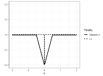
Figure 1: The clipped $L_{1}$ and $L_{0}$ penalties

3 Main results

In this section, we provide theoretical justifications of the sparse-penalized DNN estimator (5) in both regression and binary classification tasks. We prove that minimax optimal convergence rates of the excess risk can be obtained adaptively for various nonparametric regression and classification tasks.

3.1 Nonparametric regression

We first consider a nonparametric regression task, where the response $Y\in\mathbb{R}$ and input $\mathbf{X}\in[0,1]^{d}$ are generated from the model

$$Y=f^{\star}(\mathbf{X})+\epsilon,\quad\mathbf{X}\sim\mathsf{P}_{\mathbf{X}},$$ (8)

where $f^{\star}\mathrel{\mathop{\ordinarycolon}}[0,1]^{d}\mapsto\mathbb{R}$ is the unknown true regression function, $\mathsf{P}_{\mathbf{X}}$ is a distribution on $[0,1]^{d}$ and $\epsilon$ is an error variable independent to the input variable $\mathbf{X}$. For technical simplicity, we focus on the sub-Gaussian error such that

$$\mathsf{E}(\textup{e}^{t\epsilon})\leq\textup{e}^{t^{2}\sigma^{2}/2}$$ (9)

for any $t\in\mathbbm{R}$ for some $\sigma>0$. We denote by $\mathcal{P}_{\sigma,F^{\star}}$ the set of distributions $(\mathbf{X},Y)$ satisfying the model 8:

$$\mathcal{P}_{\sigma,F^{\star}}\mathrel{\mathop{\ordinarycolon}}=\mathinner{\left\{\mbox{Model \lx@cref{refnum}{eq:model_reg}}\mathrel{\mathop{\ordinarycolon}}\mathsf{E}(\textup{e}^{t\epsilon})\leq\textup{e}^{t^{2}\sigma^{2}/2},\forall t\in\mathbbm{R},\|f^{\star}\|_{\infty}\leq F^{\star}\right\}}.$$

The problem is to estimate the unknown true regression function $f^{\star}$ based on given training data $\{(\mathbf{X}_{1},Y_{i})\}_{i\in[n]}\sim\mathsf{P}^{n}$ where $\mathsf{P}\in\mathcal{P}_{a,F^{\star}}$. We evaluate the performance of an estimator $\hat{f}$ by the expected $L_{2}(\mathsf{P}_{\mathbf{X}})$ error

$$\mathsf{E}\mathinner{\left[\|\hat{f}-f^{\star}\|^{2}_{2,\mathsf{P}_{\mathbf{X}}}\right]},$$

where the expectation is taken over the training data and

$$\|\hat{f}-f^{\star}\|^{2}_{2,\mathsf{P}_{\mathbf{X}}}\mathrel{\mathop{\ordinarycolon}}=\int|\hat{f}(\mathbf{x})-f^{\star}(\mathbf{x})|^{2}\mathrm{d}\mathsf{P}_{\mathbf{X}}(\mathbf{x}).$$

The following theorem provides an oracle inequality for the expected $L_{2}(\mathsf{P}_{\mathbf{X}})$ error of the sparse-penalized DNN estimator.

Theorem 1.

Assume that the true generative model $\mathsf{P}$ is in $\mathcal{P}_{\sigma,F^{\star}}$. Let $F>0$ and let $\{L_{n}\}_{n\in\mathbbm{N}}$, $\{N_{n}\}_{n\in\mathbbm{N}}$ and $\{B_{n}\}_{n\in\mathbbm{N}}$ be positive sequences such that $L_{n}\lesssim\log n$, $N_{n}\lesssim n^{\nu_{1}}$, $1\leq B_{n}\lesssim n^{\nu_{2}}$ for some $\nu_{1},\nu_{2}>0$. Then the sparse-penalized DNN estimator defined by

$$\hat{f}_{n}\in\operatorname*{\arg\!\min}_{f\in\mathcal{F}^{\textsc{dnn}}_{n}}\mathinner{\left[\frac{1}{n}\sum_{i=1}^{n}(Y_{i}-f(\mathbf{X}_{i}))^{2}+\lambda_{n}\mathinner{\!\left\lVert\bm{\uptheta}(f)\right\rVert}_{\mathsf{clip},\tau_{n}}\right]},$$ (10)

with $\mathcal{F}^{\textsc{dnn}}_{n}=\mathcal{F}^{\textsc{dnn}}_{\rho}(L_{n},N_{n},B_{n},F)$, $\lambda_{n}\asymp\log^{5}n/n$ and $-\log\tau_{n}\geq A\log^{2}n$ for sufficiently large $A>0$, satisfies

$$\mathsf{E}\mathinner{\left[\mathinner{\lVert\hat{f}_{n}-f^{\star}\rVert}_{2,\mathsf{P}_{\mathbf{X}}}^{2}\right]}\leq 2\inf_{f\in\mathcal{F}^{\textsc{dnn}}_{n}}\mathinner{\left\{\mathinner{\!\left\lVert f-f^{\star}\right\rVert}_{2,\mathsf{P}_{\mathbf{X}}}^{2}+\lambda_{n}\mathinner{\!\left\lVert\bm{\uptheta}(f)\right\rVert}_{\mathsf{clip},\tau_{n}}\right\}}\vee\frac{C_{\sigma,F^{\star}}\log^{2}n}{n}$$ (11)

for some constant $C_{\sigma,F^{\star}}>0$ depending only on $\sigma$ and $F^{\star}$, where the expectation is taken over the training data.

The following theorem, which is a corollary of Theorem 1, provides a useful tool to derive convergence rates of the sparse-penalized DNN estimator for various classes of functions to which the true regression function $f^{\star}$ belongs.

Theorem 2.

Let $\{L_{n}\}_{n\in\mathbbm{N}}$, $\{N_{n}\}_{n\in\mathbbm{N}}$, $\{B_{n}\}_{n\in\mathbbm{N}}$ and $F>0$ be as in Theorem 1. Moreover, let $F^{\star}>0$ and let $\mathcal{F}^{\star}$ be a set of some real-valued functions on $[0,1]^{d}$. Assume that there are constants $\kappa>0$, $r>0$, $\epsilon_{0}>0$ and $C>0$ such that

$$\sup_{f^{\diamond}\in\mathcal{F}^{\star}\mathrel{\mathop{\ordinarycolon}}\|f^{\diamond}\|_{\infty}\leq F^{\star}}\inf_{f\in\mathcal{F}^{\textsc{dnn}}_{\rho}(L_{n},N_{n},B_{n},F,S_{n,\epsilon})}\|f-f^{\diamond}\|_{2,\mathsf{P}_{\mathbf{X}}}\leq\epsilon$$ (12)

with $S_{n,\epsilon}\mathrel{\mathop{\ordinarycolon}}=C\epsilon^{-\kappa}\log^{r}n$ for any $\epsilon\in(0,\epsilon_{0})$ and $n\in\mathbbm{N}.$ Then the sparse-penalized DNN estimator defined by 10 with $\mathcal{F}^{\textsc{dnn}}_{n}=\mathcal{F}^{\textsc{dnn}}_{\rho}(L_{n},N_{n},B_{n},F)$ satisfies

$$\sup_{\mathsf{P}\in\mathcal{P}_{\sigma,F^{\star}}\mathrel{\mathop{\ordinarycolon}}f^{\star}\in\mathcal{F}^{\star}}\mathsf{E}\mathinner{\left[\mathinner{\lVert\hat{f}_{n}-f^{\star}\rVert}_{2,\mathsf{P}_{\mathbf{X}}}^{2}\right]}\lesssim n^{-\frac{2}{\kappa+2}}\log^{5+r}n.$$ (13)

If there exist positive constants $\nu_{1}$ and $\nu_{2}$ in Theorem 1 with which the condition 12 holds for wide classes of $\mathcal{F}^{\star}$, then the convergence rate of the sparse-penalized estimator can be adaptive to the choice of $\mathcal{F}^{\star}.$ In the followings, we list up several examples where the sparse-penalized estimator is adaptively minimax optimal (up to a logarithmic factor). Before this, we consider the two types of activation functions given below because the constant $\nu_{2}$ differs for these two types of activation functions.

Definition 3.

A function $\rho\mathrel{\mathop{\ordinarycolon}}\mathbb{R}\to\mathbb{R}$ is continuous piecewise linear if it is continuous and there exist a finite number of break points $a_{1}\leq a_{2}\leq\cdots\leq a_{K}\in\mathbb{R}$ with $K\in\mathbbm{N}$ such that $\rho^{\prime}(a_{k}-)\neq\rho^{\prime}(a_{k}+)$ for every $k\in[K]$ and $\rho(x)$ is linear on $(-\infty,a_{1}]$, $[a_{1},a_{2}]$, $\dots$, $[a_{K-1},a_{K}]$, $[a_{K},\infty)$.

Definition 4.

A function $\rho\mathrel{\mathop{\ordinarycolon}}\mathbb{R}\to\mathbb{R}$ is locally quadratic if there exits an open interval $(a,b)\subset\mathbb{R}$ on which $\rho$ is three times continuously differentiable with bounded derivatives and there exists $t\in(a,b)$ such that $\rho^{\prime}(t)\neq 0$ and $\rho^{\prime\prime}(t)\neq 0$.

Examples of continuous piecewise linear and locally quadratic activation functions are ReLU and sigmoid functions, respectively. Other activation functions are listed in Section B.1.

Hölder functions

The Hölder space of smoothness $\alpha>0$ with radius $R>0$ is defined as

$$\mathcal{H}^{\alpha,R}(\mathcal{X})\mathrel{\mathop{\ordinarycolon}}=\left\{f\mathrel{\mathop{\ordinarycolon}}\mathcal{X}\mapsto\mathbb{R}\mathrel{\mathop{\ordinarycolon}}\|f\|_{\mathcal{H}^{\alpha}(\mathcal{X})}\leq R\right\},$$ (14)

where $\|f\|_{\mathcal{H}^{\alpha}(\mathcal{X})}$ denotes the Hölder norm defined by

$$\|f\|_{\mathcal{H}^{\alpha}(\mathcal{X})}\mathrel{\mathop{\ordinarycolon}}= \sum_{\mathbf{m}\in\mathbbm{N}_{0}^{d}\mathrel{\mathop{\ordinarycolon}}\|\mathbf{m}\|_{1}\leq\left\lfloor{\alpha}\right\rfloor}\|\partial^{\mathbf{m}}f\|_{\infty}$$

$$+\sum_{\mathbf{m}\in\mathbbm{N}_{0}^{d}\mathrel{\mathop{\ordinarycolon}}\|\mathbf{m}\|_{1}=\left\lfloor{\alpha}\right\rfloor}\sup_{\mathbf{x}_{1},\mathbf{x}_{2}\in\mathcal{X},\mathbf{x}_{1}\neq\mathbf{x}_{2}}\frac{|\partial^{\mathbf{m}}f(\mathbf{x}_{1})-\partial^{\mathbf{m}}f(\mathbf{x}_{2})|}{|\mathbf{x}_{1}-\mathbf{x}_{2}|^{\alpha-\left\lfloor{\alpha}\right\rfloor}}.$$

Here, $\partial^{\mathbf{m}}f$ denotes the partial derivative of $f$ of order $\mathbf{m}$.

Yarotsky (2017) and Schmidt-Hieber (2020) proved that for $\mathcal{H}^{\alpha,R}([0,1]^{d})$, the class of DNNs $\mathcal{F}^{\textsc{dnn}}_{\rho}(L_{n},N_{n},B_{n},F,S)$ with the ReLU activation $\rho$ and

$$L_{n}\asymp\log n,\quad N_{n}\gtrsim n^{\frac{d}{2\alpha+d}},\quad B_{n}=1,\quad F>F^{\star}$$

satisfies the condition 12 with $\kappa=d/\alpha$ and $r=1$ for all $\alpha>0.$ Hence, for $L_{n}\asymp\log n$, $N_{n}\asymp n$, $B_{n}=B\geq 1$, $F>F^{\star}$ and the ReLU activation function $\rho$, Theorem 2 implies that the convergence rate of the sparse-penalized DNN estimator defined by 10 with $\mathcal{F}^{\textsc{dnn}}_{n}=\mathcal{F}^{\textsc{dnn}}_{\rho}(L_{n},N_{n},B_{n},F)$ is given by

$$n^{-\frac{2\alpha}{2\alpha+d}}\log^{6}n,$$ (15)

which is the minimax optimal (up to a logarithmic factor). That is, the sparse-penalized DNN estimator is minimax-optimal adaptively to the smootheness $\alpha.$

Also Theorem 1 of Ohn and Kim (2019) (which is presented in Theorem 12 in Appendix B for reader’s convenience) shows that similar approximation results hold for piecewise linear activation function with $B_{n}\asymp 1$ and locally quadratic activation functions with $B_{n}\asymp n^{4}.$

Composition structured functions

The curse of dimensionality can be avoided by certain structural assumptions on the regression function. Schmidt-Hieber (2020) considered so-called composition structured regression functions which include a single-index model (Gaiffas and Lecué, 2007), an additive model (Stone, 1985; Buja et al., 1989) and a generalized additive model with an unknown link function (Horowitz et al., 2007) as special cases. This class is specified as follows. Let $q\in\mathbbm{N}$, $\mathbf{d}\mathrel{\mathop{\ordinarycolon}}=(d_{1},\dots,d_{q+1})\in\mathbbm{N}^{q+1}$ with $d_{1}\mathrel{\mathop{\ordinarycolon}}=d$ and $d_{q+1}=1$, $\mathbf{t}\mathrel{\mathop{\ordinarycolon}}=(t\textdagger_{1},\dots,t_{q+1})\in\prod_{j=1}^{q+1}[d_{j}]$, and $\bm{\alpha}\mathrel{\mathop{\ordinarycolon}}=(\alpha_{1},\dots,\alpha_{q})\in\mathbb{R}^{q}$. We denote by $\mathcal{G}^{\textsc{comp}}(q,\bm{\alpha},\mathbf{d},\mathbf{t},R)$ a set of composition structured function given by

$$\mathcal{G}^{\textsc{comp}}(q,\bm{\alpha},\mathbf{d},\mathbf{t},R)$$ (16)

$$\mathrel{\mathop{\ordinarycolon}}=\big{\{}f=g_{q}\circ\cdots\circ g_{1}\mathrel{\mathop{\ordinarycolon}}g_{j}=(g_{j,k})_{k\in[d_{j+1}]}\mathrel{\mathop{\ordinarycolon}}[a_{j},b_{j}]^{d_{j}}\mapsto[a_{j+1},b_{j+1}]^{d_{j+1}},$$

$$\hskip 113.81102ptg_{j,k}\in\mathcal{H}^{\alpha_{j},R}([a_{j},b_{j}]^{t_{j}})\mbox{ for some $|a_{j}|\vee|b_{j}|\leq R$}\big{\}}.$$

Letting $\alpha^{*}_{j}\mathrel{\mathop{\ordinarycolon}}=\alpha_{j}\prod_{h=j+1}^{q}(\alpha_{h}\wedge 1)$ for each $j\in[q-1]$ and $\alpha_{q}^{*}\mathrel{\mathop{\ordinarycolon}}=\alpha_{q}$, Schmidt-Hieber (2020) showed that for the function class $\mathcal{G}^{\textsc{comp}}(q,\bm{\alpha},\mathbf{d},\mathbf{t},R)$ in LABEL:eq:compose, the class of DNNs $\mathcal{F}^{\textsc{dnn}}_{\rho}(L_{n},N_{n},B_{n},F,S)$ with the ReLU activation $\rho$ and

$$L_{n}\asymp\log n,\quad N_{n}\gtrsim\max_{j\in[q]}n^{\frac{t_{j}}{2\alpha^{*}_{j}+t_{j}}},\quad B_{n}=1,\quad F>F^{\star}$$

satisfies the condition 12 with

$$\kappa=\max_{j\in[q]}\frac{t_{j}}{\alpha^{*}_{j}}$$

and $r=1$. Thus for $L_{n}\asymp\log n$, $N_{n}\asymp n$, $B_{n}=B\geq 1$, $F>F^{\star}$ and the ReLU activation function $\rho$, the sparse-penalized DNN estimator defined by 10 with $\mathcal{F}^{\textsc{dnn}}_{n}=\mathcal{F}^{\textsc{dnn}}_{\rho}(L_{n},N_{n},B_{n},F)$ attains the rate

$$\max_{j\in[q]}n^{-\frac{2\alpha^{*}_{j}}{2\alpha^{*}_{j}+t_{j}}}\log^{6}n,$$ (17)

which is minimax optimal up to a logarithmic factor. Theorem 15 in Appendix B shows that a similar approximation result holds for the piecewise linear activation functions with $B_{n}\asymp 1$ and hence the corresponding sparse-penalized DNN estimator is minimax optimal adaptively to $(\alpha_{j}\mathrel{\mathop{\ordinarycolon}}j\in[q])$.

For locally quadratic activation functions, a situation is tricky. In Appendix B, we succeeded in proving only that there exists $\nu_{2}>0$ satisfies Theorem 2 only when there exists $\xi>0$ such that $\min_{j\in[q]}\alpha_{j}>\xi.$ That is, the sparse-penalized DNN estimator is adaptively minimax optimal only for sufficiently smooth functions. However, we think that this minor incompleteness would be mainly due to technical limitations.

Piecewise smooth functions

Petersen and Voigtlaender (2018) and Imaizumi and Fukumizu (2019) introduced a notion of piecewise smooth functions, which have a support divided into several pieces with smooth boundaries and are smooth only within each of the pieces. Let $M\in\mathbbm{N}$, $K\in\mathbbm{N}$, $\alpha>0$, $\beta>0$ and $R>0$. Formally, the class of piecewise smooth functions is defined as

$$\mathcal{G}^{\textsc{piece}}(\alpha,\beta,M,K,R)\mathrel{\mathop{\ordinarycolon}}=\big{\{}f\mathrel{\mathop{\ordinarycolon}} f(\mathbf{x})=\sum_{m=1}^{M}g_{m}(\mathbf{x})\prod_{k\in[K]}\mathbbm{1}\mathinner{\left(x_{j_{m,k}}\geq h_{m,k}(\mathbf{x}_{-j_{m,k}})\right)},$$ (18)

$$g_{m}\in\mathcal{H}^{\alpha,R}([0,1]^{d}),h_{m,k}\in\mathcal{H}^{\beta,R}([0,1]^{d-1}),j_{m,k}\in[d]\big{\}}.$$

Petersen and Voigtlaender (2018) and Imaizumi and Fukumizu (2019) showed that for the function class $\mathcal{G}^{\textsc{piece}}(\alpha,\beta,M,K,R)$ in 18, the class of DNNs $\mathcal{F}^{\textsc{dnn}}_{\rho}(L_{n},N_{n},B_{n},F,S)$ with the ReLU activation function and

$$L_{n}\asymp\log n,\quad N_{n}\gtrsim n^{\frac{d}{2\alpha+d}}\vee n^{\frac{d-1}{\beta+d-1}},\quad B_{n}\gtrsim n^{\frac{\alpha}{2\alpha+d}}\vee n^{\frac{\beta}{2(\beta+d-1)}},\quad F>F^{\star}$$

satisfies the condition 12 with

$$\kappa=\frac{d}{\alpha}\vee\frac{2(d-1)}{\beta}$$

and $r=1$, provided that the marginal distribution $\mathsf{P}_{\mathbf{X}}$ of the input variable admits a density $\frac{\mathrm{d}\mathsf{P}_{\mathbf{X}}}{\mathrm{d}\mu}$ with respect to the Lebesgue measure $\mu$ and $\sup_{\mathbf{x}\in[0,1]^{d}}\frac{\mathrm{d}\mathsf{P}_{\mathbf{X}}}{\mathrm{d}\mu}(\mathbf{x})\leq C$ for some $C>0$. Hence for $L_{n}\asymp\log n$, $N_{n}\asymp n$, $B_{n}\asymp n$, $F>F^{\star}$ and the ReLU activation function $\rho$, the sparse-penalized DNN estimator defined by 10 with $\mathcal{F}^{\textsc{dnn}}_{n}=\mathcal{F}^{\textsc{dnn}}_{\rho}(L_{n},N_{n},B_{n},F)$ attains the rate

$$\mathinner{\left\{n^{-\frac{2\alpha}{2\alpha+d}}\vee n^{-\frac{\beta}{\beta+d-1}}\right\}}\log^{6}n,$$ (19)

which is minimax optimal up to a logarithmic factor.

Theorem 17 in Appendix B shows that a similar DNN approximation result holds for piecewise linear activation functions with $B_{n}\asymp n$ and locally quadratic activation functions with $B_{n}\asymp n^{4}$. Hence the sparse-penalized DNN estimator with the activation function being either piecewise linear or locally quadratic is also minimax optimal adaptively to $\alpha$ and $\beta$.

Besov and mixed smooth Besov functions

Suzuki (2019) proved the minimax optimality of the ERM estimator with a certain sparsity constraint for the estimation of a regression function in the Besov space or the mixed smooth Besov space. Similarly to the other function spaces, we can prove that the sparse-penalized DNN estimator is minimax optimal adaptively for the Besov space or the mixed smooth Besov space using Theorem 2 along with Proposition 1 and Theorem 1 of Suzuki (2019), respectively. We omit the details due to the limitation of spaces.

Summary of the network architecture

In Table 1, we summarize the minimal values of the network architecture parameters $\nu_{1}$ and $\nu_{2}$ that attain the adaptive optimality according to the type of activation function and the class of true regression functions. Note that any values of the architecture parameters larger than the corresponding minimal values in the table also lead to the adaptive optimality. Thus, users can select $\nu_{1}$ and $\nu_{2}$ based on the prior information about the true regression function and the results in the table without resorting to a tuning procedure. The choice $\nu_{1}=1$ is allowed regardless of the true regression function and the choice of the activation function. Any $\nu_{1}$ larger than 1 can be used but additional computation is needed since more hidden nodes are used. For $\nu_{2}$, we may need a very large value, in particular, when we use the locally quadratic activation function and the true regression function is of composition structured. But since the boundness restriction of the parameter does not affect its computational complexity and thus we recommend to use a sufficiently large $\nu_{2}.$

Table 1: Summary of the minimal values of the network architecture parameters $\nu_{1}$ and $\nu_{2}$ that attain the adaptive optimality according to the activation function and the class of true regression functions. Here, $\xi$ denotes the lower bound of the smoothness $(\alpha_{j}\mathrel{\mathop{\ordinarycolon}}j\in[q]).$

True regression function	Activation function	$\nu_{1}$	$\nu_{2}$
Hölder smooth	Piecewise linear	1	0
	Locally quadratic	1	4
Composition structured	Piecewise linear	1	0
	Locally quadratic	1	$4+\frac{1}{2}\max\{0,\xi^{-q+1}-4\}$
Piecewise smooth	Piecewise linear	1	1
	Locally quadratic	1	4

3.2 Classification with strictly convex losses

In this section, we consider a binary classification problem. The goal of classification is to find a real-valued function $f$ (called a decision function) such that $f(\mathbf{x})$ is a good prediction of the label $y\in\{-1,1\}$ for a new sample $(\mathbf{x},y)$. In practice, the margin-based loss function, which evaluates the quality of the prediction by $f$ for a sample $(\mathbf{x},y)$ based on its margin $yf(\mathbf{x})$, is popularly used. Examples of the margin based loss functions are the 0-1 loss $\mathbbm{1}(yf(\mathbf{x})<0)$, hinge loss $(1-yf(\mathbf{x}))\vee 0$, exponential loss $\exp(-yf(\mathbf{x}))$ and logistic loss $\log(1+\exp(-yf(\mathbf{x})))$. Here we focus on strictly convex losses which include the exponential and the logistic losses. Note that the logistic loss is popularly used for learning a DNN classifier in practice under the name of cross-entropy.

We assume that the label $Y\in\{-1,1\}$ and input $\mathbf{X}\in[0,1]^{d}$ are generated from the model

$$Y|\mathbf{X}=\mathbf{x}\sim 2\mathsf{Bernoulli}(\eta(\mathbf{x}))-1,\quad\mathbf{X}\sim\mathsf{P}_{\mathbf{X}},$$ (20)

where $\eta(\mathbf{x})$ is called a conditional class probability and $\mathsf{P}_{\mathbf{X}}$ is a distribution on $[0,1]^{d}$. The aim is to find a real-valued function $f$ so that the excess risk of $f$ given by:

$$\mathcal{E}_{\mathsf{P}}(f)\mathrel{\mathop{\ordinarycolon}}=\mathsf{E}(\ell(Yf(\mathbf{X})))-\mathsf{E}(\ell(Yf_{\ell}^{\star}(\mathbf{X})))$$

close to zero as possible, where $\ell$ is a given margin-based loss function, $f_{\ell}^{\star}=\operatorname*{\arg\!\min}_{f\in\mathcal{F}}\mathsf{E}(\ell(Yf(\mathbf{X})))$ is the optimal decision function and $\mathcal{F}$ is a set of all real-valued measurable functions on $[0,1]^{d}$. We assume that $\|f_{\ell}^{\star}\|_{\infty}\leq F^{\star}$ for some $F^{\star}>0$. This assumption is satisfied if the conditional class probability $\eta(\mathbf{x})$ satisfies $\inf_{\mathbf{x}\in[0,1]^{d}}\eta(\mathbf{x})\wedge(1-\eta(\mathbf{x}))\geq\eta_{0}$ for some $\eta_{0}>0$, i.e., $\eta$ is bounded away from 0 and 1, for the exponential and logistic losses. This is because $f_{\ell}^{\star}(\mathbf{x})=\log(\eta(\mathbf{x})/(1-\eta(\mathbf{x}))).$ We denote by $\mathcal{Q}_{F^{\star}}$ the set of distributions satisfying the above assumption, that is,

$$\mathcal{Q}_{F^{\star}}=\mathinner{\left\{\mbox{Model \lx@cref{refnum}{eq:model_reg_cls}}\mathrel{\mathop{\ordinarycolon}}\|f_{\ell}^{\star}\|_{\infty}\leq F^{\star}\right\}}.$$

The following theorem states the oracle inequality for the excess risk of the sparse-penalized DNN estimator based on a strictly convex margin-based loss function.

Theorem 5.

Let $\ell$ be a strictly convex margin-based loss function with continuous first and second derivatives. Assume that the true generative model $\mathsf{P}$ is in $\mathcal{Q}_{F^{\star}}$. Let $F>0$ and let $\{L_{n}\}_{n\in\mathbbm{N}}$, $\{N_{n}\}_{n\in\mathbbm{N}}$ and $\{B_{n}\}_{n\in\mathbbm{N}}$ be positive sequences such that $L_{n}\lesssim\log n$, $N_{n}\lesssim n^{\nu_{1}}$, $1\leq B_{n}\lesssim n^{\nu_{2}}$ for some $\nu_{1},\nu_{2}>0$. Then the sparse-penalized DNN estimator defined by

$$\hat{f}_{n}\in\operatorname*{\arg\!\min}_{f\in\mathcal{F}^{\textsc{dnn}}_{n}}\mathinner{\left[\frac{1}{n}\sum_{i=1}^{n}\ell(Y_{i}f(\mathbf{X}_{i}))+\lambda_{n}\mathinner{\!\left\lVert\bm{\uptheta}(f)\right\rVert}_{\mathsf{clip},\tau_{n}}\right]}$$ (21)

with $\mathcal{F}^{\textsc{dnn}}_{n}=\mathcal{F}^{\textsc{dnn}}_{\rho}(L_{n},N_{n},B_{n},F)$, $\lambda_{n}\asymp\log^{3}n/n$ and $-\log\tau_{n}\geq A\log^{2}n$ for sufficiently large $A>0$, satisfies

$$\mathsf{E}\mathinner{\left[\mathcal{E}_{\mathsf{P}}(\hat{f}_{n})\right]}\leq 2\inf_{f\in\mathcal{F}^{\textsc{dnn}}_{n}}\mathinner{\left\{\mathcal{E}_{\mathsf{P}}(f)+\lambda_{n}\mathinner{\!\left\lVert\bm{\uptheta}(f)\right\rVert}_{\mathsf{clip},\tau_{n}}\right\}}\vee\frac{C\log n}{n},$$ (22)

for some universal constant $C>0$, where the expectation is taken over the training data.

The following theorem, which is a corollary of Theorem 5, is an extension of Theorem 2 for strictly convex margin-based loss functions.

Theorem 6.

Let $\{L_{n}\}_{n\in\mathbbm{N}}$, $\{N_{n}\}_{n\in\mathbbm{N}}$ and $\{B_{n}\}_{n\in\mathbbm{N}}$ and $F>0$ be as in Theorem 5. Moreover, let $F^{\star}>0$ and let $\mathcal{F}^{\star}$ be a set of some real-valued functions on $[0,1]^{d}$. Assume that there are constants $\kappa>0$, $r>0$, $\epsilon_{0}>0$ and $C>0$ such that

$$\sup_{f^{\diamond}\in\mathcal{F}^{\star}\mathrel{\mathop{\ordinarycolon}}\|f^{\diamond}\|_{\infty}\leq F^{\star}}\inf_{f\in\mathcal{F}^{\textsc{dnn}}_{\rho}(L_{n},N_{n},B_{n},F,S_{n,\epsilon})}\|f-f^{\diamond}\|_{2,\mathsf{P}_{\mathbf{X}}}\leq\epsilon,$$ (23)

with $S_{n,\epsilon}\mathrel{\mathop{\ordinarycolon}}=C\epsilon^{-\kappa}\log^{r}n$ for any $\epsilon\in(0,\epsilon_{0})$ and $n\in\mathbbm{N}.$ Then the sparse-penalized DNN estimator defined by 21 with $\mathcal{F}^{\textsc{dnn}}_{n}=\mathcal{F}^{\textsc{dnn}}_{\rho}(L_{n},N_{n},B_{n},F)$ satisfies

$$\sup_{\mathsf{P}\in\mathcal{Q}_{F^{\star}}\mathrel{\mathop{\ordinarycolon}}f_{\ell}^{\star}\in\mathcal{F}^{\star}}\mathsf{E}\mathinner{\left[\mathcal{E}_{\mathsf{P}}(\hat{f}_{n})\right]}\lesssim n^{-\frac{2}{\kappa+2}}\log^{3+r}n.$$ (24)

As is done in Section 3.1, we can obtain the convergence rate of the excess risk using Theorem 6 when the optimal decision function $f_{\ell}^{\star}$ belongs to one of the function classes considered in Section 3.1. For example, if the optimal decision function $f_{\ell}^{\star}$ is in Hölder space with smoothness $\alpha>0$, the the excess risk of the sparse-penalized DNN estimator defined by 21 with a piecewise linear activation function and $\nu_{2}=0$ converges to zero at a rate $n^{-\frac{2\alpha}{2\alpha+d}}\log^{4}n$.

4 Computation

In this section, we propose a scalable optimization algorithm to solve the problem 5. Due to the nonlinearity of DNNs, finding the global optimum of 5 is almost impossible. There are various gradient based optimization algorithms which effectively reduce the empirical risk $\mathcal{L}_{n}(\bm{\uptheta})\mathrel{\mathop{\ordinarycolon}}=n^{-1}\sum_{i=1}^{n}\ell(Y_{i},f(\mathbf{X}_{i}|\bm{\uptheta}))$ (Duchi et al., 2011; Kingma and Ba, 2014; Luo et al., 2019; Liu et al., 2019), where $f(\cdot|\bm{\uptheta})$ denotes the DNN with parameter $\bm{\uptheta}$. These algorithms, however, would not work well since not only the empirical risk but also the penalty are nonconvex. To make the problem simpler, we propose to replace the clipped $L_{1}$ penalty by its convex tight upper bound. The idea of using the convex upper bound is proposed under the name of the CCCP (Yuille and Rangarajan, 2003), the difference of convex functions (DC) programming (Tao and An, 1997) and the majorize-minimization (MM) algorithm (Lange, 2013).

Note that the clipped $L_{1}$ penalty is decomposed as the sum of the convex and concave parts as

$$\|\bm{\uptheta}\|_{\mathsf{clip},\tau}\mathrel{\mathop{\ordinarycolon}}=\sum_{j=1}^{p}\left(\frac{|\theta_{j}|}{\tau}\wedge 1\right)=\frac{1}{\tau}\sum_{j=1}^{p}|\theta_{j}|-\frac{1}{\tau}\sum_{j=1}^{p}(|\theta_{j}|-\tau)\mathbbm{1}(|\theta_{j}|\geq\tau),$$ (25)

where $p$ denotes the dimension of $\bm{\uptheta}$ and the first term of the right-hand side is convex while the second term is concave in $\bm{\uptheta}$. For given current solution $\hat{\bm{\uptheta}}^{(t)},$ the tight convex upper bound of the second term $-\frac{1}{\tau}\sum_{j=1}^{p}(|\theta_{j}|-\tau)\mathbbm{1}(|\theta_{j}|\geq\tau)$ at the current solution $\hat{\theta}^{(t)}_{j}$ is given as

$$-\frac{1}{\tau}\sum_{j=1}^{p}\textup{sign}\mathinner{\left(\hat{\theta}^{(t)}_{j}\right)}\mathinner{\left(\theta_{j}-\tau\right)}\mathbbm{1}\mathinner{\left(|\hat{\theta}^{(t)}_{j}|>\tau\right)}.$$ (26)

By replacing $-\frac{1}{\tau}\sum_{j=1}^{p}(|\theta_{j}|-\tau)\mathbbm{1}(|\theta_{j}|\geq\tau)$ with the tight convex upper bound 26, the objective function becomes

$$Q^{*}(\bm{\uptheta}|\hat{\bm{\uptheta}}^{(t)})\mathrel{\mathop{\ordinarycolon}}=\mathcal{L}_{n}(\bm{\uptheta})-\left\langle{\frac{\lambda}{\tau}\mathbf{h}_{\tau}^{(t)}},{\bm{\uptheta}-\tau\mathbf{1}}\right\rangle+\frac{\lambda}{\tau}\|\bm{\uptheta}\|_{1},$$ (27)

where

$$\mathbf{h}_{\tau}^{(t)}\mathrel{\mathop{\ordinarycolon}}=\mathinner{\bigl{(}\textup{sign}(\hat{\bm{\uptheta}}^{(t)}_{j})\mathbbm{1}\mathinner{(|\hat{\bm{\uptheta}}^{(t)}_{j}|>\tau)}\bigr{)}}_{j\in[p]}.$$

The following proposition justifies the use of 27.

Proposition 7.

For any parameter $\tilde{\bm{\uptheta}}$ satisfying $Q^{*}(\tilde{\bm{\uptheta}}|\hat{\bm{\uptheta}}^{(t)})\leq Q^{*}(\hat{\bm{\uptheta}}^{(t)}|\hat{\bm{\uptheta}}^{(t)})$, we have $Q(\tilde{\bm{\uptheta}})\leq Q(\hat{\bm{\uptheta}}^{(t)}),$ where

$$Q(\bm{\uptheta})\mathrel{\mathop{\ordinarycolon}}=\mathcal{L}_{n}(\bm{\uptheta})+\lambda\|\bm{\uptheta}\|_{\mathsf{clip},\tau}.$$

Proof.

By definition of $Q^{*}(\cdot|\hat{\bm{\uptheta}}^{(t)})$, $Q^{*}(\hat{\bm{\uptheta}}^{(t)}|\hat{\bm{\uptheta}}^{(t)})=Q(\hat{\bm{\uptheta}}^{(t)})$ and $Q(\tilde{\bm{\uptheta}})\leq Q^{*}(\tilde{\bm{\uptheta}}|\hat{\bm{\uptheta}}^{(t)})$, which lead to the desired result. ∎

We apply the proximal gradient descent algorithm (Parikh et al., 2014) to minimize $Q^{*}(\bm{\uptheta}|\hat{\bm{\uptheta}}^{(t)})$. That is, we iteratively update the solution as

$$\hat{\bm{\uptheta}}^{(t,k+1)}=\operatorname*{\arg\!\min}_{\bm{\uptheta}}\mathinner{\left[\frac{\lambda}{\tau}\|\bm{\uptheta}\|_{1}+\left\langle{\nabla\mathcal{L}_{n}(\hat{\bm{\uptheta}}^{(t,k)})-\frac{\lambda}{\tau}\mathbf{h}_{\tau}^{(t)}},{\bm{\uptheta}}\right\rangle+\frac{1}{2\eta_{t}}\mathinner{\!\left\lVert\bm{\uptheta}-\hat{\bm{\uptheta}}^{(t,k)}\right\rVert}_{2}^{2}\right]}$$ (28)

for $k\in\mathbbm{N}_{0}$ with $\hat{\bm{\uptheta}}^{(t,0)}\mathrel{\mathop{\ordinarycolon}}=\hat{\bm{\uptheta}}^{(t)},$ where $\nabla\mathcal{L}_{n}(\hat{\bm{\uptheta}}^{(t,k)})$ is the gradient of $\mathcal{L}_{n}(\bm{\uptheta})$ at $\bm{\uptheta}=\hat{\bm{\uptheta}}^{(t,k)}$ and $\eta_{t}$ is a pre-specified learning rate. Then, we let $\hat{\bm{\uptheta}}^{(t+1)}=\hat{\bm{\uptheta}}^{(t,k_{t}^{*}+1)},$ where

$$k_{t}^{*}\mathrel{\mathop{\ordinarycolon}}=\inf\mathinner{\left\{k\in\mathbbm{N}_{0}\mathrel{\mathop{\ordinarycolon}}Q^{*}\mathinner{\bigl{(}\hat{\bm{\uptheta}}^{(t,k+1)}|\hat{\bm{\uptheta}}^{(t)}\bigr{)}}\leq Q^{*}\mathinner{\bigl{(}\hat{\bm{\uptheta}}^{(t)}|\hat{\bm{\uptheta}}^{(t)}\bigr{)}}\right\}}\wedge\bar{k},$$

and $\bar{k}$ is the pre-specified maximum number of iterations. The proximal gradient algorithm is known to reduce $Q^{*}(\bm{\uptheta}|\hat{\bm{\uptheta}}^{(t)})$ well and thus the proposed algorithm which combines the CCCP and proximal gradient descent algorithm is expected to decrease the objective function $Q(\bm{\uptheta})$ monotonically by Proposition 7. As an empirical evidence, Figure 2 draws the curve of the objective function value versus iteration number for a simulated data, which amply shows the monotonicity of our algorithm.

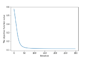
Figure 2: The objective function value versus iteration

Note that 28 has the closed form solution given as

$$\hat{\theta}^{(t,k+1)}_{j}=\mathinner{\left(u_{\tau,\lambda,j}^{(t,k)}-\textup{sign}(u_{\tau,\lambda,j}^{(t,k)})\eta_{t}\frac{\lambda}{\tau}\right)}\mathbbm{1}\mathinner{\left(\mathinner{\!\left\lvert u_{\tau,\lambda,j}^{(t,k)}\right\rvert}\geq\eta_{t}\frac{\lambda}{\tau}\right)},$$ (29)

where

$$u_{\tau,\lambda,j}^{(t,k)}\mathrel{\mathop{\ordinarycolon}}=\hat{\theta}_{j}^{(t,k)}-\eta_{t}\mathinner{\left(\nabla\mathcal{L}_{n}(\hat{\bm{\uptheta}}^{(t,k)})_{j}-\frac{\lambda}{\tau}h_{\tau,j}^{(t)}\right)}$$

for $j\in[p]$. The solution 29 is a soft-thresholded version of $u_{\tau,\lambda,j}^{(t,k)}$, which is sparse. Thus we can obtain a sparse estimate of the DNN parameter during the training procedure without any post-training pruning algorithm such as Han et al. (2015); Li et al. (2016).

5 Numerical studies

5.1 Regression with simulated data

In this section, we carry out simulation studies to illustrate the finite-sample performance of the sparse-penalized DNN estimator (SDNN). We compare the sparse-penalized DNN estimator with other popularly used regression estimators: kernel ridge regression (KRR), $k$-nearest neighbors (kNN), random forest (RF), and non-sparse DNN (NSDNN).

For kernel ridge regression we used a radial basis function (RBF) kernel. For both the non-sparse and sparse DNN estimators, we used a network architecture of 5 hidden layers with the numbers of hidden nodes $(100,100,100,100,100)$. The non-sparse DNN is learned with popularly used optimizing algorithm Adam (Kingma and Ba, 2014) with learning rate $10^{-3}$.

We select tuning parameters associated with each estimator by optimizing the performance on a held-out validation data set whose size is one fifth of the size of the training data. The tuning parameters include the scale parameter of the RBF kernel, a degree of regularization for kernel ridge regression, the number of neighbors for $k$-nearest neighbors, the depth of the trees for the random forest and the two tuning parameters $\lambda$ and $\tau$ in the clipped $L_{1}$ penalty.

We first generate 10-dimensional input $\mathbf{x}$ from the uniform distribution on $[0,1]^{10},$ and generate the corresponding response $Y$ from $Y=f^{\star}(\mathbf{x})+\epsilon$ for some function $f^{\star}$, where $\epsilon$ is a standard normal error. The functions used for $f^{\star}$ are as listed below:

$$f_{1}^{\star}(\mathbf{x}) =c_{1}\sum_{j=1}^{10}(-1)^{j}j^{-1}x_{j}$$

$$f_{2}^{\star}(\mathbf{x}) =c_{2}\sin(\|\mathbf{x}\|_{1})$$

$$f_{3}^{\star}(\mathbf{x}) =c_{3}\mathinner{\left[x_{1}x_{2}^{2}-x_{3}+\log\mathinner{\left(x_{4}+4x_{5}+\exp(x_{6}x_{7}-5x_{5})\right)}+\tan(x_{8}+0.1)\right]}$$

$$f_{4}^{\star}(\mathbf{x}) =c_{4}\mathinner{\left[\exp\mathinner{\left(3x_{1}+x_{2}^{2}-\sqrt{x_{3}+5}\right)}+0.01\cot\mathinner{\left(\frac{1}{0.01+|x_{4}-2x_{5}+x_{6}|}\right)}\right]}$$

$$f_{5}^{\star}(\mathbf{x}) =c_{5}\mathinner{\left[3\exp(\|\mathbf{x}\|_{2})\mathbbm{1}\mathinner{\left(x_{2}\geq x_{3}^{2}\right)}+x_{3}^{x_{4}}-x_{5}x_{6}x_{7}^{4}\right]}$$

$$f_{6}^{\star}(\mathbf{x}) =c_{6}\big{[}4x_{1}x_{2}x_{3}x_{4}\mathbbm{1}\mathinner{\left(x_{3}+x_{4}\geq 1,x_{5}\geq x_{6}\right)}+\tan(\|\mathbf{x}\|_{1})\mathbbm{1}\mathinner{\left(x_{1}^{2}x_{7}x_{8}\geq x_{9}x_{10}^{3}\right)}\big{]}.$$

The functions $f_{1}^{\star}$ and $f_{2}^{\star}$ are globally smooth functions, $f_{3}^{\star}$ and $f_{4}^{\star}$ are composition structured functions and $f_{5}^{\star}$ and $f_{6}^{\star}$ are piecewise smooth functions. The constants $c_{1},\dots,c_{6}$ are chosen so that the error variance becomes $5\%$ of the variance of the response.

The performance of each estimator is measured by the empirical $L_{2}$ error computed based on newly generated $10^{5}$ simulated data. Figure 3 draws the boxplots of the empirical $L_{2}$ errors of the 5 estimators over 50 simulation replicates for the six true functions. We see that the sparse-penalized DNN estimator outperforms the other competing estimators for the all 6 true functions, even though it is less stable compared to the other stable estimators (KRR, KNN and RF).

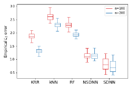
(a) $f_{1}^{\star}$

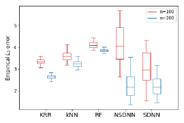
(b) $f_{2}^{\star}$

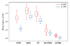
(c) $f_{3}^{\star}$

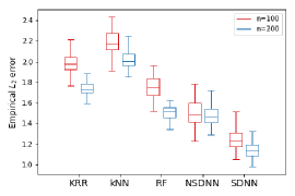
(d) $f_{4}^{\star}$

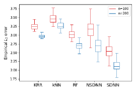
(e) $f_{5}^{\star}$

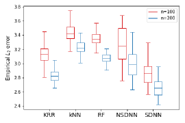
(f) $f_{6}^{\star}$

Figure 3: Simulation results for the true functions $f_{1}^{\star},\dots,f_{6}^{\star}$, respectively. We draw the boxplots of the empirical $L_{2}$ errors of the 5 estimators from 50 simulation replicates.

Table 2 presents the sparsity, which is defined as the percentage of non-zero parameters, of the sparse-penalized DNN estimate for each simulation setup. The sparsity ranges from 20% for estimating the simple linear function $f_{1}^{\star}$ to 68% for estimating the more complex piecewise smooth function $f_{5}^{\star}$. This result indicates that the sparse-penalized DNN estimator can improve the prediction accuracy compared to the non-sparse DNN by removing redundant parameters adaptively to the “complexity” of the true function, as our theory suggests.

Table 2: The averaged sparsity (the percentage of non-zero parameters) and standard deviation in the paranthesis over 50 simulation replicates.

True function	Sample size
	$n=100$	$n=200$
$f_{1}^{\star}$	22.87% (4.21%)	20.5% (3.4%)
$f_{2}^{\star}$	52.96% (8.67%)	58.27% (8.69%)
$f_{3}^{\star}$	45.23% (7.88%)	47.16% (5.24%)
$f_{4}^{\star}$	37.38% (6.95%)	39.29% (6.93%)
$f_{5}^{\star}$	65.94% (9.12%)	67.43% (8.65%)
$f_{6}^{\star}$	61.56% (10.64%)	67.0% (8.46%)

5.2 Classification with real data sets

We compare the sparse-penalized DNN estimator with other competing estimators by analyzing the following four data sets from the UCI repository:

• Haberman: Haberman’s survival data set contains 306 patients who had undergone surgery for breast cancer at the University of Chicago’s Billings Hospital. The task is to predict whether each patient survives after 5 years after the surgery or not.

• Retinopathy: This data set contains features extracted from 1,151 eye’s images. The task is to predict whether an eye’s image contains signs of diabetic retinopathy or not based on the other features.

• Tic-tac-toe: This data set contains all the 957 possible board configurations at the end of tic-tac-toe games which are encoded to 27 input variables. The task it to predict the winner of the game.

• Promoter: This data set consists of A, C, G, T nucleotides at 57 positions for 106 gene sequences, and each nucleotide is encoded to a 3-dimensional one-hot vector. The task is to predict whether a gene is promoters or non-promoter.

For competing estimators, we considered a support vector machine (SVN), $k$-nearest neighbors (kNN), random forest (RF), and non-sparse DNN (NSDNN). For the support vector machine, we used the RBF kernel. The tuning parameters in each methods are selected by evaluation on a validation data set whose size is one fifth of the size of whole training data.

We splits the whole data into training and test data sets with the ratio 7:3, then evaluate the classification accuracy of each learned estimator on the test data set. We repeat this splits 50 times. Table 3 presents the averaged classification accuracy over 50 training-test splits. The proposed sparse-penalized DNN estimator is the best for Tic-tac-toe and Promoter data sets, and the second best for the other two data sets. Moreover, the sparse-penalized DNN estimator is similarly stable to the other competitors.

Table 3: The averaged classification accuracies and standard errors in the paranthesis over 50 training-test splits of the four UCI data sets.

Data	Haberman	Retinopathy	Tic-tac-toe	Promoter
$(n,d)$	(214, 3)	(805, 19)	(669, 27)	(74, 171)
SVM	0.7298 (0.0367)	0.5737 (0.0282)	0.8467 (0.0243)	0.7887 (0.1041)
kNN	0.7587 (0.0366)	0.6436 (0.0263)	0.9714 (0.0102)	0.8012 (0.0649)
RF	0.7365 (0.0377)	0.665 (0.0263)	0.9777 (0.0103)	0.8725 (0.0582)
NSDNN	0.7328 (0.0464)	0.7158 (0.0293)	0.9735 (0.0107)	0.8594 (0.062)
SDNN	0.752 (0.0382)	0.6987 (0.0375)	0.98 (0.0085)	0.8769 (0.0474)

To understand the suboptimal accuracy of the sparse-penalized DNN estimator for the two data sets Haberman and Retinopathy, which are of relatively low input dimensional, we conduct an additional toy experiment that examines an effect of the input dimension. We consider the following probability model for generating simulated data. For a given input dimension $d\in\mathbbm{N}$, let $\mathbf{X}$ be a random vector following the uniform distribution on $[0,1]^{d}$. Then for a given $\mathbf{X}=\mathbf{x}$, the random variable $Y\in\{-1,1\}$ has the probability mass $\mathsf{P}(Y=1|\mathbf{X}=\mathbf{x})=(1+\exp(-g^{\star}(\mathbf{x})))^{-1}$, where $g^{\star}$ is a function given by

$$g^{\star}(\mathbf{x})=\sum_{j=1}^{\left\lfloor{d/2}\right\rfloor}x_{j}^{2}-\mu$$

for a constant $\mu\in\mathbb{R}$. We choose $\mu$ so that $\mathsf{E}g^{\star}(\mathbf{X})=0$. For each input dimension $d\in\{5,20,35,50\}$, we generate 50 training data sets with size $n=100$ from the above probability model. Then we apply the five estimators considered in this section to the simulated data sets and obtain classification accuracies computed on the test data set independently generated from the same probability model.

The result is presented in Figure 4, where the averaged classification accuracies over 50 simulation replicates for each estimators are reported. For the smallest $d,$ the non-DNN estimators perform better than both the non-sparse and sparse-penalized DNN estimators. However, as the input dimension increases, the performance of the sparse-penalized DNN estimator is improved quickly and it becomes superior to the other competitors. This result explains partly why the sparse-penalized DNN estimator does not perform best for the two low dimensional data sets Haberman $(d=3)$ and Retinopathy $(d=19)$.

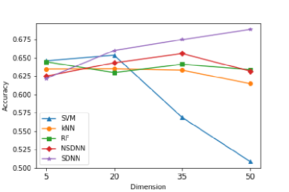
Figure 4: The averaged classification accuracies over 50 simulation replicates with varying input dimensions.

6 Conclusion

In this paper, we proposed a sparse-penalized DNN estimator leaned with the clipped $L_{1}$ penalty and proved the theoretical optimiality. An interesting conclusion is that the sparse-penalized DNN estimator is extremely flexible so that it achieves the optimal minimax convergence rate (up to a logarithmic factor) without using any information about the true function for various situations. Moreover, we proposed an efficient and scalable optimization algorithm so that the sparse-penalized DNN estimator can be used in practice without much difficulty.

There are several possible future works. For binary classification, we only consider the strictly convex losses which are popular in learning DNNs. We have not considered convex but not strictly convex losses such as the hinge loss. We expect that the sparse-penalized DNN estimator learned with the hinge loss and the clipped $L_{1}$ penalty can attain the minimax optimal convergence rates for estimation of a decision boundary.

In this paper, we only considered a fully connected DNN. We may use a more structured architecture such as the convolutional neural network when the information of the structure of the true function is available. It would be interesting to investigating how much structured neural networks are helpful compared to simple fully connected neural networks.

Theoretical properties of generative models such as generative adversarial networks (Goodfellow et al., 2014) and variational autoencoders (Kingma and Welling, 2013) have not been fully studied even though some results are available (Liang, 2018; Briol et al., 2019; Uppal et al., 2019). A difficulty in generative models would be that we have to work with functions where the dimension of the range is larger than the dimension of the domain.

Appendix A Proofs

For notational simplicity, we only consider a 1-Lipschitz activation function $\rho$ with $\rho(0)=0$. Extensions of the proofs for general $C$-Lipschitz activation functions with arbitrary value of $\rho(0)$ can be done easily.

A.1 Covering numbers of the DNN classes

We provide a covering number bound for a class of DNNs with a certain sparsity constraint. Let $\mathcal{F}$ be a given class of real-valued functions defined on $\mathcal{X}$. Let $\delta>0$. A collection $\{f_{i}\mathrel{\mathop{\ordinarycolon}}i\in[N]\}$ is called a $\delta$-covering set of $\mathcal{F}$ with respect to the norm $\|\cdot\|$ if, for all $f\in\mathcal{F}$, there exists $f_{i}$ in the collection such that $\|f-f_{i}\|\leq\delta$. The cardinality of the minimal $\delta$-covering set is called the $\delta$-covering number of $\mathcal{F}$ with respect to the norm $\|\cdot\|$ , and is denoted by $\mathcal{N}(\delta,\mathcal{F},\|\cdot\|)$. The following proposition gives the covering number bound of the class of DNNs with the $L_{0}$ sparsity constraint.

Proposition 8 (Proposition 1 of Ohn and Kim (2019)).

Let $L\in\mathbbm{N}$, $N\in\mathbbm{N}$, $B\geq 1$, $F>0$ and $S>0$. Then for any $\delta>0$,

$$\log\mathcal{N}\mathinner{\left(\delta,\mathcal{F}_{\rho}^{\textsc{dnn}}(L,N,B,F,S),\|\cdot\|_{\infty}\right)}\leq 2S(L+1)\log\mathinner{\left(\frac{(L+1)(N+1)B}{\delta}\right)}.$$ (30)

The following lemma is a technical one.

Lemma 9.

Let $L\in\mathbbm{N}$, $N\in\mathbbm{N}$ and $B\geq 1.$ For any two DNNs $f_{1},f_{2}\in\mathcal{F}_{\rho}(L,N,B,\infty)$, we have

$$\|f_{1}-f_{2}\|_{\infty,[0,1]^{d}}\leq(L+1)(B(N+1))^{L+1}\mathinner{\!\left\lVert\bm{\uptheta}(f_{1})-\bm{\uptheta}(f_{2})\right\rVert}_{\infty}$$

Proof.

For $f\in\mathcal{F}_{\rho}(L,N,B,\infty)$ expressed as

$$f(\mathbf{x})=A_{L+1}\circ\rho_{L}\circ A_{L}\circ\cdots\circ\rho_{1}\circ A_{1}(\mathbf{x}),$$

we define $[f]_{l}^{-}\mathrel{\mathop{\ordinarycolon}}[0,1]^{d}\mapsto\mathbb{R}^{N-1}$ and $[f]_{l}^{+}\mathrel{\mathop{\ordinarycolon}}\mathbb{R}^{N-1}\mapsto\mathbb{R}$ for $l\in\{2,\dots,L\}$ by

$$[f]^{-}_{l}(\cdot) \mathrel{\mathop{\ordinarycolon}}=\rho_{l-1}\circ A_{l-1}\circ\cdots\circ\rho_{1}\circ A_{1}(\cdot),$$

$$[f]^{+}_{l}(\cdot) \mathrel{\mathop{\ordinarycolon}}=A_{L+1}\circ\rho_{L}\circ A_{L}\circ\cdots\rho_{l}\circ\mathsf{A}_{l}\circ\rho_{l-1}(\cdot).$$

Corresponding to the last and first layer, we define $f^{-}_{1}(\mathbf{x})=\mathbf{x}$ and $f^{+}_{L+2}(\mathbf{x})=\mathbf{x}$. Note that $f=[f]^{+}_{l+1}\circ A_{l}\circ[f]^{-}_{l}$.

Let $\mathbf{W}_{l}$ and $\mathbf{b}_{l}$ be the weight matrix and bias vector at the $l$-th hidden layer of $f$. Note that both the numbers of rows and columns of $\mathbf{W}_{l}$ are less than $N-1$. Thus for any $\mathbf{x}\in[0,1]^{d}$

$$\mathinner{\!\left\lVert[f]^{-}_{l}(\mathbf{x})\right\rVert}_{\infty} \leq\mathinner{\!\left\lVert\mathbf{W}_{l-1}[f]^{-}_{l-1}(\mathbf{x})+\mathbf{b}_{l-1}\right\rVert}_{\infty}$$

$$\leq(N+1)B\mathinner{\lVert[f]^{-}_{l-1}(\mathbf{x})\rVert}_{\infty}+B$$

$$\leq(N+1)B\mathinner{\left(\mathinner{\lVert[f]^{-}_{l-1}(\mathbf{x})\rVert}_{\infty}\vee 1\right)}$$

$$\leq(N+1)B\mathinner{\left(((N+1)B\mathinner{\lVert[f]^{-}_{l-2}(\mathbf{x})\rVert}_{\infty}\vee 1)\vee 1\right)}$$

$$\leq((N+1)B)^{2}\mathinner{\left(\mathinner{\lVert[f]^{-}_{l-2}(\mathbf{x})\rVert}_{\infty}\vee 1\right)}$$

$$\leq((N+1)B)^{l-1}\mathinner{\left(\mathinner{\lVert\mathbf{x}\rVert}_{\infty}\vee 1\right)}$$

$$=((N+1)B)^{l-1},$$

where the fifth inequality follows from the assumption that $(N+1)B\geq 1$. Similarly, we can show that for any $\mathbf{z}_{1},\mathbf{z}_{2}\in\mathbb{R}^{N}$,

$$\mathinner{\!\left\lvert[f]^{+}_{l+1}(\mathbf{z}_{1})-[f]^{+}_{l+1}(\mathbf{z}_{2})\right\rvert}\leq((N+1)B)^{L+1-l}\|\mathbf{z}_{1}-\mathbf{z}_{2}\|_{\infty}.$$

For $f_{1},f_{2}\in\mathcal{F}_{\rho}(L,N,B,\infty)$, letting $A_{j,l}$ be the affine transform at the $l$-th hidden layer of $f_{j}$ for $j=1,2$, we have for any $\mathbf{x}\in[0,1]^{d}$,

$$|f_{1}(\mathbf{x})-f_{2}(\mathbf{x})| \leq\mathinner{\!\left\lvert\sum_{l=1}^{L+1}\mathinner{\left[[f_{1}]^{+}_{l+1}\circ A_{1,l}\circ[f_{2}]^{-}_{l}(\mathbf{x})-[f_{1}]^{+}_{l+1}\circ A_{2,l}\circ[f_{2}]^{-}_{l}(\mathbf{x})\right]}\right\rvert}$$

$$\leq\sum_{l=1}^{L+1}((N+1)B)^{L+1-l}\mathinner{\!\left\lVert(A_{1,l}-A_{2,l})\circ[f_{2}]^{-}_{l}(\mathbf{x})\right\rVert}_{\infty}$$

$$\leq\sum_{l=1}^{L+1}((N+1)B)^{L+1-l}\|\bm{\uptheta}(f_{1})-\bm{\uptheta}(f_{2})\|_{\infty}\mathinner{\left\{N\mathinner{\!\left\lVert[f_{2}]^{-}_{l}(\mathbf{x})\right\rVert}_{\infty}+1\right\}}$$

$$\leq\sum_{l=1}^{L+1}((N+1)B)^{L+1-l}\|\bm{\uptheta}(f_{1})-\bm{\uptheta}(f_{2})\|_{\infty}\mathinner{\left\{N((N+1)B)^{l-1}+1\right\}}$$

$$\leq(L+1)((N+1)B)^{L+1}\|\bm{\uptheta}(f_{1})-\bm{\uptheta}(f_{2})\|_{\infty},$$

which completes the proof. ∎

Using Proposition 8 and Lemma 9 we can compute an upper bound of the $\delta$-covering number of a class of DNNs with a restriction on the clipped $L_{1}$ norm when $\delta$ is not too small, which is stated in the following proposition.

Proposition 10.

Let $L\in\mathbbm{N}$, $N\in\mathbbm{N}$, $B\geq 1$, $F>0$ and $\tau>0.$ Let

$$\check{\mathcal{F}}_{\rho,\tau}^{\textsc{dnn}}(L,N,B,F,S) \mathrel{\mathop{\ordinarycolon}}=\mathinner{\left\{f\in\mathcal{F}_{\rho}^{\textsc{dnn}}(L,N,B,F)\mathrel{\mathop{\ordinarycolon}}\|\bm{\uptheta}(f)\|_{\mathsf{clip},\tau}\leq S\right\}}.$$

Then we have that for any $\delta>\tau(L+1)((N+1)B)^{L+1}$,

$$\log\mathcal{N}\mathinner{\left(\delta,\check{\mathcal{F}}_{\rho,\tau}^{\textsc{dnn}}(L,N,B,F,S),\|\cdot\|_{\infty}\right)}$$ (31)

$$\leq\log\mathcal{N}\mathinner{\left(\delta-\tau(L+1)((N+1)B)^{L+1},\mathcal{F}_{\rho}^{\textsc{dnn}}(L,N,B,F,S),\|\cdot\|_{\infty}\right)}$$

$$\leq 2S(L+1)\log\mathinner{\left(\frac{(L+1)(N+1)B}{\delta-\tau(L+1)((N+1)B)^{L+1}}\right)}.$$

Proof.

For a DNN $f$ with parameter $\bm{\uptheta}(f)$, we let $f^{(\tau)}$ be the DNN constructed by the parameter which is the hard thresholding of $\bm{\uptheta}(f)$ with the threshold $\tau$, that is, $\bm{\uptheta}(f^{(\tau)})=\bm{\uptheta}(f)\mathbbm{1}(|\bm{\uptheta}(f)|>\tau)$. Then by Lemma 9,

$$\mathinner{\lVert f-f^{(\tau)}\rVert}_{\infty} \leq(L+1)((N+1)B)^{L+1}\mathinner{\lVert\bm{\uptheta}(f)-\bm{\uptheta}(f^{(\tau)})\rVert}_{\infty}$$

$$\leq\tau(L+1)((N+1)B)^{L+1}.$$

Given $\delta>(L+1)((N+1)B)^{L+1}$, let $\delta^{*}\mathrel{\mathop{\ordinarycolon}}=\delta-(L+1)((N+1)B)^{L+1}>0$ and let $\{f_{j}^{0}\mathrel{\mathop{\ordinarycolon}}j\in[N_{\delta^{*}}]\}$ be the minimal $\delta^{*}$-covering set of $\mathcal{F}_{\rho}^{\textsc{dnn}}(L,N,B,F,S)$ with respect to the norm $\|\cdot\|_{\infty}$, where

$$N_{\delta^{*}}\mathrel{\mathop{\ordinarycolon}}=\mathcal{N}(\delta^{*},\mathcal{F}_{\rho}^{\textsc{dnn}}(L,N,B,F,S),\|\cdot\|_{\infty}).$$

Since $\|\bm{\uptheta}(f^{(\tau)})\|_{0}=\|\bm{\uptheta}(f^{(\tau)})\|_{\mathsf{clip},\tau}\leq\|\bm{\uptheta}(f)\|_{\mathsf{clip},\tau}\leq S$, it follows that $f^{(\tau)}\in\mathcal{F}_{\rho}^{\textsc{dnn}}(L,N,B,F,S)$ for any $f\in\check{\mathcal{F}}_{\rho,\tau}^{\textsc{dnn}}(L,N,B,F,S)$. Hence for any $f\in\check{\mathcal{F}}_{\rho,\tau}^{\textsc{dnn}}(L,N,B,F,S)$, there is $j\in[N_{\delta^{*}}]$ such that $\mathinner{\lVert f^{(\tau)}-f_{j}^{0}\rVert}_{\infty}\leq\delta^{*}$ and so

$$\mathinner{\lVert f-f_{j}^{0}\rVert}_{\infty} \leq\mathinner{\lVert f-f^{(\tau)}\rVert}_{\infty}+\mathinner{\lVert f^{(\tau)}-f_{j}^{0}\rVert}_{\infty}$$

$$\leq\tau(L+1)((N+1)B)^{L+1}+\delta^{*}=\delta,$$

which implies that $\{f_{j}^{0}\mathrel{\mathop{\ordinarycolon}}j\in[N_{\delta^{*}}]\}$ is also a $\delta$-covering set of $\check{\mathcal{F}}_{\rho,\tau}^{\textsc{dnn}}(L,N,B,F,S)$. By Proposition 8, the proof is done. ∎

A.2 Proofs of Theorem 1 and Theorem 5

Let $\mathsf{P}_{n}$ be the empirical distribution based on the data $(\mathbf{X}_{1},Y_{1}),\dots,(\mathbf{X}_{n},Y_{n})$. We use the abbreviation $\mathsf{Q}f\mathrel{\mathop{\ordinarycolon}}=\int f\mathrm{d}\mathsf{Q}$ for a measurable function $f$ and measure $\mathsf{Q}$. Throughout this section, $\mathcal{F}_{n}^{\textsc{dnn}}\mathrel{\mathop{\ordinarycolon}}=\mathcal{F}_{\rho}^{\textsc{dnn}}(L_{n},N_{n},B_{n},F)$ and $J_{\lambda_{n},\tau_{n}}(\cdot)\mathrel{\mathop{\ordinarycolon}}=\lambda_{n}\|\bm{\uptheta}(\cdot)\|_{\mathsf{clip},\tau_{n}}$.

For the proofs of Theorem 1 and Theorem 5, we need the following large deviation bound for empirical processes. This is a slight modification of Theorem 19.3 of Györfi et al. (2006) that states the result with the covering number with respect to the empirical $L_{2}$ norm. Since the empirical $L_{2}$ norm is always less than the $L_{\infty}$ norm, the following lemma is a direct consequence of Theorem 19.3 of Györfi et al. (2006).

Lemma 11 (Theorem 19.3 of Györfi et al. (2006)).

Let $K_{1}\geq 1$ and $K_{2}\geq 1$. Let $\mathbf{Z}_{1},\dots,\mathbf{Z}_{n}$ be independent and identically distributed random variables with values in $\mathcal{Z}$ and let $\mathcal{G}$ be a class of functions $g\mathrel{\mathop{\ordinarycolon}}\mathcal{Z}\mapsto\mathbb{R}$ with the properties $\|g\|_{\infty}\leq K_{1}$ and $\mathsf{E}g(\mathbf{Z})^{2}\leq K_{2}\mathsf{E}g(\mathbf{Z})$. Let $\omega\in(0,1)$ and $t^{*}>0$. Assume that

$$\sqrt{n}\omega\sqrt{1-\omega}\sqrt{t^{*}}\geq 288\max\{2K_{1},\sqrt{2K_{2}}\}$$ (32)

and that any $\delta\geq t^{*}/8$,

$$\frac{\sqrt{n}\omega(1-\omega)\delta}{96\sqrt{2}\max\{K_{1},2K_{2}\}}\geq\int_{\frac{\omega(1-\omega)\delta}{16\max\{K_{1},2K_{2}\}}}^{\sqrt{\delta}}\sqrt{\log\mathcal{N}\mathinner{\left(u,\mathcal{G},\|\cdot\|_{\infty}\right)}}\mathrm{d}u.$$ (33)

Then

$$\mathsf{P}\mathinner{\left(\sup_{g\in\mathcal{G}}\frac{\mathinner{\!\left\lvert(\mathsf{P}-\mathsf{P}_{n})g\right\rvert}}{t^{*}+\mathsf{P}g}\geq\omega\right)}\leq 60\exp\mathinner{\left(-\frac{nt^{*}\omega^{2}(1-\omega)}{128\cdot 2304\max\{K_{1}^{2},K_{2}\}}\right)}.$$

Proof of Theorem 1.

Throughout the proof, when comparing two positive sequences $\{a_{n}\}_{n\in\mathbbm{N}}$ and $\{b_{n}\}_{n\in\mathbbm{N}}$, we write $a_{n}\lesssim_{\sigma,F^{\star}}b_{n}$ if there is a constant $C_{\sigma,F^{\star}}>0$ depending only on $\sigma$ and $F^{\star}$ such that $a_{n}\leq C_{\sigma,F^{\star}}b_{n}$ for any $n\in\mathbbm{N}$.

Let $K_{n}\mathrel{\mathop{\ordinarycolon}}=(\sqrt{32\sigma^{2}}\log^{1/2}n)\vee F$. Let $Y^{\dagger}\mathrel{\mathop{\ordinarycolon}}=\text{sign}(Y)(|Y|\wedge K_{n}),$ which is a truncated version of $Y$ and $f^{\dagger}$ be the regression function of $Y^{\dagger}$, that is,

$$f^{\dagger}(\mathbf{x})\mathrel{\mathop{\ordinarycolon}}=\mathsf{E}(Y^{\dagger}|\mathbf{X}=\mathbf{x}).$$

We suppress the dependency on $n$ in the notation $Y^{\dagger}$ and $f^{\dagger}$ for notational convenience. We start with the decomposition

$$\mathinner{\lVert\hat{f}_{n}-f^{*}\rVert}^{2}_{2,\mathsf{P}_{\mathbf{X}}}=\mathsf{P}(Y-\hat{f}_{n}(\mathbf{X}))^{2}-\mathsf{P}(Y-f^{\star}(\mathbf{X}))^{2}=\sum_{i=1}^{4}A_{i,n},$$ (34)

where

$$A_{1,n} \mathrel{\mathop{\ordinarycolon}}=\mathinner{\left[\mathsf{P}(Y-\hat{f}_{n}(\mathbf{X}))^{2}-\mathsf{P}(Y-f^{\star}(\mathbf{X}))^{2}\right]}$$

$$\qquad-\mathinner{\left[\mathsf{P}(Y^{\dagger}-\hat{f}_{n}(\mathbf{X}))^{2}-\mathsf{P}(Y^{\dagger}-f^{\dagger}(\mathbf{X}))^{2}\right]}$$

$$A_{2,n} \mathrel{\mathop{\ordinarycolon}}=\mathinner{\left[\mathsf{P}(Y^{\dagger}-\hat{f}_{n}(\mathbf{X}))^{2}-\mathsf{P}(Y^{\dagger}-f^{\dagger}(\mathbf{X}))^{2}\right]}$$

$$\qquad-2\mathinner{\left[\mathsf{P}_{n}(Y^{\dagger}-\hat{f}_{n}(\mathbf{X}))^{2}-\mathsf{P}_{n}(Y^{\dagger}-f^{\dagger}(\mathbf{X}))^{2}\right]}-2J_{\lambda_{n},\tau_{n}}(\hat{f}_{n})$$

$$A_{3,n} \mathrel{\mathop{\ordinarycolon}}=2\mathinner{\left[\mathsf{P}_{n}(Y^{\dagger}-\hat{f}(\mathbf{X}))^{2}-\mathsf{P}_{n}(Y^{\dagger}-f^{\dagger}(\mathbf{X}))^{2}\right]}$$

$$\qquad-2\mathinner{\left[\mathsf{P}_{n}(Y-\hat{f}(\mathbf{X}))^{2}-\mathsf{P}_{n}(Y-f^{\star}(\mathbf{X}))^{2}\right]}$$

$$A_{4,n} \mathrel{\mathop{\ordinarycolon}}=2\mathinner{\left[\mathsf{P}_{n}(Y-\hat{f}(\mathbf{X}))^{2}-\mathsf{P}_{n}(Y-f^{\star}(\mathbf{X}))^{2}\right]}+2J_{\lambda_{n},\tau_{n}}(\hat{f}_{n}).$$

To bound $A_{1,n}$, we first recall that well-known properties of sub-Gaussian variables such that the condition 9 implies that $\mathsf{P}\epsilon=0$ and $\mathsf{E}\textup{e}^{\epsilon^{2}/(4\sigma^{2})}\leq\sqrt{2}$, e.g., see Theorem 2.6 of Wainwright (2019). Let

$$A_{1,1,n} \mathrel{\mathop{\ordinarycolon}}=\mathsf{P}\mathinner{\left((Y^{\dagger}-Y)(2\hat{f}_{n}(\mathbf{X})-Y-Y^{\dagger})\right)},$$

$$A_{1,2,n} \mathrel{\mathop{\ordinarycolon}}=\mathsf{P}\mathinner{\left\{\mathinner{\left(Y^{\dagger}-f^{\dagger}(\mathbf{X}))-Y+f^{\star}(\mathbf{X})\right)}\mathinner{\left(Y^{\dagger}-f^{\dagger}(\mathbf{X})+Y-f^{\star}(\mathbf{X})\right)}\right\}}$$

so that $A_{1,n}=A_{1,1,n}+A_{1,2,n}$. We use the Cauchy-Schwarz inequality to get

$$|A_{1,1,n}|\leq\sqrt{\mathsf{P}\mathinner{\left(Y^{\dagger}-Y\right)}^{2}}\sqrt{\mathsf{P}\mathinner{\left(2\hat{f}_{n}(\mathbf{X})-Y-Y^{\dagger}\right)}^{2}}.$$

Since $\mathsf{E}\textup{e}^{Y^{2}/(8\sigma^{2})}\leq\textup{e}^{(F^{\star})^{2}/(4\sigma^{2})}\mathsf{E}\textup{e}^{\epsilon^{2}/(4\sigma^{2})}\leq\sqrt{2}\textup{e}^{(F^{\star})^{2}/(4\sigma^{2})}$, we have that

$$\mathsf{P}\mathinner{(Y^{\dagger}-Y)}^{2} =\mathsf{P}[|Y|^{2}\mathbbm{1}(|Y|>K_{n})]$$ (35)

$$\leq\mathsf{P}[16\sigma^{2}\textup{e}^{Y^{2}/(16\sigma^{2})}\textup{e}^{Y^{2}/(16\sigma^{2})-K_{n}^{2}/(16\sigma^{2})}]$$

$$\leq 16\sqrt{2}\sigma^{2}\textup{e}^{(F^{\star})^{2}/(4\sigma^{2})}\textup{e}^{-2\log n}=16\sqrt{2}\sigma^{2}\textup{e}^{(F^{\star})^{2}/(4\sigma^{2})}n^{-2},$$

and that

$$\mathsf{P}\mathinner{\left(2\hat{f}_{n}(\mathbf{X})-Y-Y^{\dagger}\right)}^{2} \leq 2\mathsf{P}(Y^{2})+2\mathsf{P}(2\hat{f}_{n}(\mathbf{X})-Y^{\dagger})^{2}$$ (36)

$$\leq 16\sigma^{2}\mathsf{E}\textup{e}^{Y^{2}/(8\sigma^{2})}+18K_{n}^{2}$$

$$\lesssim_{\sigma,F^{\star}}\log n.$$

Thus $|A_{1,1,n}|\lesssim_{\sigma,F^{\star}}\log n/n$. For $A_{1,2,n}$, using the Cauchy-Schwarz inequality we have

$$|A_{1,2,n}| \leq\sqrt{2\mathsf{P}(Y^{\dagger}-Y)^{2}+2\mathsf{P}(f^{\dagger}(\mathbf{X})-f^{\star}(\mathbf{X}))^{2}}$$

$$\quad\times\sqrt{\mathsf{P}(Y+Y^{\dagger}-f^{\dagger}(\mathbf{X})-f^{\star}(\mathbf{X}))^{2}}.$$

Using the similar arguments as 36, we have $\mathsf{P}(Y+Y^{\dagger}-f^{\dagger}(\mathbf{X})-f^{\star}(\mathbf{X}))^{2}\lesssim_{\sigma,F^{\star}}\log n$. Since $\mathsf{P}\epsilon=0$, by Jensen’s inequality,

$$\mathsf{P}(f^{\dagger}(\mathbf{X})-f^{\star}(\mathbf{X}))^{2}=\mathsf{P}(\mathsf{P}(Y^{\dagger}|\mathbf{X})-\mathsf{P}(Y|\mathbf{X}))^{2}\leq\mathsf{P}(Y^{\dagger}-Y)^{2}.$$

Thus the inequality 35 concludes that $|A_{1,2,n}|\lesssim_{\sigma,F^{\star}}\log n/n$.

The term $\mathsf{E}(A_{3,n})$ can be shown to be bounded above by $\log n/n$ up to a constant depending only on $\sigma$ and $F^{\star}$ similarly to the derivations used for bounding $A_{1,n}$.

For $A_{2,n}$, define $\Delta(f)(\mathbf{Z})\mathrel{\mathop{\ordinarycolon}}=(Y^{\dagger}-f(\mathbf{X}))^{2}-(Y^{\dagger}-f^{\dagger}(\mathbf{X}))^{2}$ with $\mathbf{Z}\mathrel{\mathop{\ordinarycolon}}=(\mathbf{X},Y)$ for $f\in\mathcal{F}.$ For $t>0$, we can write

$$\mathsf{P}(A_{2,n}>t) \leq\mathsf{P}\mathinner{\left(\sup_{f\in\mathcal{F}^{\textsc{dnn}}_{n}}\frac{(\mathsf{P}-\mathsf{P}_{n})\Delta(f)(\mathbf{Z})}{t+2J_{\lambda_{n},\tau_{n}}(f)+\mathsf{P}\Delta(f)(\mathbf{Z})}\geq\frac{1}{2}\right)}$$

$$\leq\sum_{j=0}^{\infty}\mathsf{P}\mathinner{\left(\sup_{f\in\mathcal{F}_{n,j,t}}\frac{(\mathsf{P}-\mathsf{P}_{n})\Delta(f)(\mathbf{Z})}{2^{j}t+\mathsf{P}\Delta(f)(\mathbf{Z})}\geq\frac{1}{2}\right)},$$

where we define

$$\mathcal{F}_{n,j,t}\mathrel{\mathop{\ordinarycolon}}=\mathinner{\left\{f\in\mathcal{F}^{\textsc{dnn}}_{n}\mathrel{\mathop{\ordinarycolon}}2^{j-1}\mathbbm{1}(j\neq 0)t\leq J_{\lambda_{n},\tau_{n}}(f)\leq 2^{j}t\right\}}.$$

We now apply Lemma 11 to the class of functions

$$\mathcal{G}_{n,j,t}\mathrel{\mathop{\ordinarycolon}}=\mathinner{\left\{\Delta(f)\mathrel{\mathop{\ordinarycolon}}[0,1]^{d}\times\mathbb{R}\mapsto\mathbb{R}\mathrel{\mathop{\ordinarycolon}}f\in\mathcal{F}_{n,j,t}\right\}}.$$

We will check the conditions of Lemma 11. First for sufficiently large $n$, we have that for every $g\in\mathcal{G}_{n,j,t}$ with $\mathinner{\!\left\lVert g\right\rVert}_{\infty}\leq 8K_{n}^{2},$

$$\mathsf{P}(g(\mathbf{Z}))^{2} =\mathsf{P}(Y^{\dagger}-f(\mathbf{X})-(Y^{\dagger}-f^{\dagger}(\mathbf{X})))^{2}(Y^{\dagger}-f(\mathbf{X})+(Y^{\dagger}-f^{\dagger}(\mathbf{X})))^{2}$$

$$\leq 4(K_{n}+F)^{2}\mathsf{P}(f(\mathbf{X})-f^{\dagger}(\mathbf{X}))^{2}$$

$$\leq 16K_{n}^{2}\mathsf{P}g(\mathbf{Z}).$$

Thus, the condition 32 holds for any sufficiently large $n$ if $t\gtrsim\log^{2}n/n$. For the condition 33, we observe that

$$\mathinner{\!\left\lvert(y^{\dagger}-f_{1}(\mathbf{x}))^{2}-(y^{\dagger}-f^{\dagger}(\mathbf{x}))^{2}-\mathinner{\left\{(y^{\dagger}-f_{2}(\mathbf{x}))^{2}-(y^{\dagger}-f^{\dagger}(\mathbf{x}))^{2}\right\}}\right\rvert}$$

$$\leq|f_{1}(\mathbf{x})-f_{2}(\mathbf{x})||f_{1}(\mathbf{x})+f_{2}(\mathbf{x})-2y^{\dagger}|$$

$$\leq 4K_{n}|f_{1}(\mathbf{x})-f_{2}(\mathbf{x})|$$

for any $f_{1},f_{2}\in\mathcal{F}_{n,j,t}$ and $(\mathbf{x},y)\in[0,1]^{d}\times\mathbb{R}$ and so we have

$$\mathcal{N}\mathinner{\left(u,\mathcal{G}_{n,j,t},\|\cdot\|_{\infty}\right)}\leq\mathcal{N}\mathinner{\left(u/(4K_{n}),\mathcal{F}_{n,j,t},\|\cdot\|_{\infty}\right)}.$$

Let $\zeta_{n}\mathrel{\mathop{\ordinarycolon}}=(L_{n}+1)((N_{n}+1)B_{n})^{L_{n}+1}$. With $\omega=1/2$, by Proposition 10 and the assumption that $-\log\tau_{n}\geq A\log^{2}n$ for sufficiently large $A>0$ which implies $\tau_{n}\zeta_{n}\lesssim n^{-1}$, we have that for any $\delta\geq n^{-1}\log^{2}n\gtrsim 2^{13}K_{n}^{3}\tau_{n}\zeta_{n}$,

$$\int^{\sqrt{\delta}}_{\delta/(2^{11}K_{n}^{2})}\log^{1/2}\mathcal{N}\mathinner{\left(\frac{u}{4K_{n}},\mathcal{F}_{n,j,t},\|\cdot\|_{\infty}\right)}\mathrm{d}u$$ (37)

$$\leq\sqrt{\delta}\log^{1/2}\mathcal{N}\mathinner{\left(\frac{\delta}{2^{13}K_{n}^{3}},\mathcal{F}_{n,j,t},\|\cdot\|_{\infty}\right)}$$

$$\leq\sqrt{\delta}\log^{1/2}\mathcal{N}\mathinner{\left(\frac{\delta}{2^{13}K_{n}^{3}}-\tau_{n}\zeta_{n},\mathcal{F}_{\rho}^{\textsc{dnn}}(L_{n},N_{n},B_{n},F,2^{j}t/\lambda_{n}),\|\cdot\|_{\infty}\right)}$$

$$\leq 2\sqrt{\delta}(2^{j}t/\lambda_{n})^{1/2}(L_{n}+1)^{1/2}\log^{1/2}\mathinner{\left(\frac{(L_{n}+1)(N_{n}+1)B_{n}}{\delta/(2^{13}K_{n}^{3})-\tau_{n}\zeta_{n}}\right)}$$

$$\leq c_{1}\sqrt{\delta}\sqrt{2^{j}t}\frac{\sqrt{n}}{\log^{3/2}n}$$

for any sufficiently large $n$ for some constant $c_{1}>0$. Note that the constant $c_{1}$ does not depends on $j$. Then for any $t\geq t_{n}\mathrel{\mathop{\ordinarycolon}}=8\log^{2}n/n$ and any $\delta\geq 2^{j}t/8\geq\log^{2}n/n$, there exists an universal constant $c_{2}>0$ such that

$$\frac{\delta}{\log n}\geq c_{2}\frac{\sqrt{\delta}\sqrt{2^{j}t}}{\log^{3/2}n},$$ (38)

for any $j=0,1,\dots$, and thus the condition 33 is met for any $j=0,1,\dots$ and all sufficiently large $n$. Therefore we have

$$\mathsf{P}(A_{2,n}>t)\lesssim\sum_{j=0}^{\infty}\exp\mathinner{\left(-c_{3}2^{j}\frac{nt}{\log n}\right)}\lesssim\exp\mathinner{\left(-c_{3}\frac{nt}{\log n}\right)}$$

for $t\geq t_{n}$, which implies

$$\mathsf{E}(A_{2,n}) \leq 2t_{n}+\int_{2t_{n}}^{\infty}\mathsf{P}(A_{2,n}>t)\mathrm{d}t$$

$$\lesssim\frac{\log^{2}n}{n}+\frac{\log n}{n}\textup{e}^{-c_{4}\log n}\lesssim\frac{\log^{2}n}{n}$$

for some positive constants $c_{3}$ and $c_{4}$.

For $A_{4,n}$, we choose a neural network function $f_{n}^{\circ}\in\mathcal{F}^{\textsc{dnn}}_{n}$ such that

$$\mathinner{\!\left\lVert f_{n}^{\circ}-f^{\star}\right\rVert}_{2,\mathsf{P}_{\mathbf{X}}}^{2}+J_{\lambda_{n},\tau_{n}}(f_{n}^{\circ})\leq\inf_{f\in\mathcal{F}^{\textsc{dnn}}_{n}}\mathinner{\left[\mathinner{\!\left\lVert f-f^{\star}\right\rVert}_{2,\mathsf{P}_{\mathbf{X}}}^{2}+J_{\lambda_{n},\tau_{n}}(f)\right]}+n^{-1}.$$

Then by the basic inequality $\mathsf{P}_{n}(Y-\hat{f}_{n})^{2}+J_{\lambda_{n},\tau_{n}}(\hat{f}_{n})\leq\mathsf{P}_{n}(Y-f)^{2}+J_{\lambda_{n},\tau_{n}}(f)$ for any $f\in\mathcal{F}^{\textsc{dnn}}_{n}$, we have

$$A_{4,n} \leq 2\mathinner{\left[\mathsf{P}_{n}(Y-\hat{f}_{n}(\mathbf{X}))^{2}-\mathsf{P}_{n}(Y-f_{n}^{\circ}(\mathbf{X}))^{2}\right]}+2J_{\lambda_{n},\tau_{n}}(\hat{f}_{n})$$

$$\quad+2\mathinner{\left[\mathsf{P}_{n}(Y-f_{n}^{\circ}(\mathbf{X}))^{2}-\mathsf{P}_{n}(Y-f^{\star}(\mathbf{X}))^{2}\right]}$$

$$\leq 2J_{\lambda_{n},\tau_{n}}(f_{n}^{\circ})+2\mathinner{\left[\mathsf{P}_{n}(Y-f_{n}^{\circ}(\mathbf{X}))^{2}-\mathsf{P}_{n}(Y-f^{\star}(\mathbf{X}))^{2}\right]}$$

and so

$$\mathsf{E}(A_{4,n}) \leq 2J_{\lambda_{n},\tau_{n}}(f_{n}^{\circ})+2\mathinner{\!\left\lVert f_{n}^{\circ}-f^{\star}\right\rVert}^{2}_{2,\mathsf{P}_{\mathbf{X}}}$$

$$\leq 2\inf_{f\in\mathcal{F}^{\textsc{dnn}}_{n}}\mathinner{\left[\mathinner{\!\left\lVert f-f^{\star}\right\rVert}^{2}_{2,\mathsf{P}_{\mathbf{X}}}+J_{\lambda_{n},\tau_{n}}(f)\right]}+\frac{1}{n}.$$

Combining all the bounds we have derived, we get the desired result. ∎

Proof of Theorem 5.

Since $\ell$ is continuously differentiable, $\ell$ is Lipschitz on any closed interval. That is, there is a constant $c_{1}>0$ such that

$$|\ell(z_{1})-\ell(z_{2})|\leq c_{1}|z_{1}-z_{2}|$$ (39)

for any $z_{1},z_{2}\in[-F,F]$. On the other hand, since $F\geq F^{\star}$, there is a constant $c_{2}>0$ such that

$$\mathsf{E}\left\{\ell(Yf(\mathbf{X}))-\ell(Yf_{\ell}^{\star}(\mathbf{X}))\right\}^{2}\leq c_{2}\mathsf{E}\left\{\ell(Yf(\mathbf{X}))-\ell(Yf_{\ell}^{\star}(\mathbf{X}))\right\}$$ (40)

for any $f\in\{f\in\mathcal{F}\mathrel{\mathop{\ordinarycolon}}\|f\|_{\infty}\leq F\}$. This is a well known fact about the strictly convex losses and the proof can be found in Lemma 6.1 of Park (2009).

We decompose $\mathcal{E}_{\mathsf{P}}(\hat{f}_{n})$ as

$$\mathcal{E}_{\mathsf{P}}(\hat{f}_{n})=\mathsf{P}\ell(Y\hat{f}_{n}(\mathbf{X}))-\mathsf{P}\ell(Yf_{\ell}^{\star}(\mathbf{X}))=B_{1,n}+B_{2,n},$$

where

$$B_{1,n} \mathrel{\mathop{\ordinarycolon}}=\mathinner{\left[\mathsf{P}\ell(Y\hat{f}_{n}(\mathbf{X}))-\mathsf{P}\ell(Yf^{\star}(\mathbf{X}))\right]}$$

$$\quad-2\mathinner{\left[\mathsf{P}_{n}\ell(Y\hat{f}_{n}(\mathbf{X}))-\mathsf{P}_{n}\ell(Yf^{\star}(\mathbf{X}))\right]}-2J_{\lambda_{n},\tau_{n}}(\hat{f}_{n})$$

$$B_{2,n} \mathrel{\mathop{\ordinarycolon}}=2\mathinner{\left[\mathsf{P}_{n}\ell(Y\hat{f}_{n}(\mathbf{X}))-\mathsf{P}_{n}\ell(Yf^{\star}(\mathbf{X}))\right]}+2J_{\lambda_{n},\tau_{n}}(\hat{f}_{n}).$$

We bound $B_{1,n}$ by using a similar argument for bounding $A_{2,n}$ in the proof of Theorem 1. Let $\Delta(f)(\mathbf{Z})\mathrel{\mathop{\ordinarycolon}}=\ell(Yf(\mathbf{X}))-\ell(Yf^{\star}(\mathbf{X}))$ with $\mathbf{Z}\mathrel{\mathop{\ordinarycolon}}=(\mathbf{X},Y)$ and let

$$\mathcal{F}_{n,j,t}\mathrel{\mathop{\ordinarycolon}}=\mathinner{\left\{f\in\mathcal{F}^{\textsc{dnn}}_{n}\mathrel{\mathop{\ordinarycolon}}2^{j-1}\mathbbm{1}(j\neq 0)t\leq J_{\lambda_{n},\tau_{n}}(f)\leq 2^{j}t\right\}}.$$

Then for $t>0$, we can write

$$\mathsf{P}(B_{1,n}>t) \leq\mathsf{P}\mathinner{\left(\sup_{f\in\mathcal{F}^{\textsc{dnn}}_{n}}\frac{(\mathsf{P}-\mathsf{P}_{n})\Delta(f)(\mathbf{Z})}{t+2J_{\lambda_{n},\tau_{n}}(f)+\mathsf{P}\Delta(f)(\mathbf{Z})}\geq\frac{1}{2}\right)}$$

$$\leq\sum_{j=0}^{\infty}\mathsf{P}\mathinner{\left(\sup_{f\in\mathcal{F}_{n,j,t}}\frac{(\mathsf{P}-\mathsf{P}_{n})\Delta(f)(\mathbf{Z})}{2^{j}t+\mathsf{P}\Delta(f)(\mathbf{Z})}\geq\frac{1}{2}\right)}.$$

We now apply Lemma 11 to the class of functions

$$\mathcal{G}_{n,j,t}\mathrel{\mathop{\ordinarycolon}}=\mathinner{\left\{\Delta(f)\mathrel{\mathop{\ordinarycolon}}[0,1]^{d}\times\{-1,1\}\mapsto\mathbb{R}\mathrel{\mathop{\ordinarycolon}}f\in\mathcal{F}_{n,j,t}\right\}},$$

By 39 and 40, we can set $K_{1}=2c_{1}F$ and $K_{2}=c_{2}$ in Lemma 11. The condition 32 holds for any sufficiently large $n$ if $t\gtrsim\log n/n$. For the condition 33, we let $K^{\prime}\mathrel{\mathop{\ordinarycolon}}=K_{1}\vee 2K_{2}=(2c_{1}F)\vee 2c_{2}$ for notational simplicity. Further, let $\zeta_{n}\mathrel{\mathop{\ordinarycolon}}=(L_{n}+1)((N_{n}+1)B_{n})^{L_{n}+1}.$ Then since $\ell$ is locally Lipschitz, using a similar argument to that used for LABEL:eq:ent_bound in the proof of Theorem 1, we can show that, for any $\delta\geq n^{-1}\log n\gtrsim 4c_{2}K^{\prime}\tau_{n}\zeta_{n}$,

$$\int^{\sqrt{\delta}}_{\delta/(4K^{\prime})}\log^{1/2}\mathcal{N}\mathinner{\left(u,\mathcal{G}_{n,j,t},\|\cdot\|_{\infty}\right)}\mathrm{d}u$$

$$\leq\int^{\sqrt{\delta}}_{\delta/(4K^{\prime})}\log^{1/2}\mathcal{N}\mathinner{\left(u/c_{2},\mathcal{G}_{n,j,t},\|\cdot\|_{\infty}\right)}\mathrm{d}u$$

$$\leq\sqrt{\delta}(2^{j}t/\lambda_{n})^{1/2}L_{n}^{1/2}\log^{1/2}\mathinner{\left(\frac{(L_{n}+1)(N_{n}+1)B_{n}}{\delta/(4c_{2}K^{\prime})-\tau_{n}\zeta_{n}}\right)}$$

$$\leq c_{3}\sqrt{\delta}\sqrt{2^{j}t}\frac{\sqrt{n}}{\log^{1/2}n}$$

for all sufficiently large $n$ for some constant $c_{3}>0$. For any $t\geq t_{n}\mathrel{\mathop{\ordinarycolon}}=8n^{-1}\log n$ and any $\delta\geq 2^{j}t/8\geq n^{-1}\log n$, there exists a constant $c_{4}>0$ such that $\delta\geq c_{4}\sqrt{\delta}\sqrt{2^{j}t}/\log^{1/2}n$ for any $j=0,1,\dots,$. Thus condition 33 is met and then we have

$$\mathsf{E}(B_{1,n}) \leq 2t_{n}+\int_{2t_{n}}^{\infty}\mathsf{P}(B_{1,n}>t)\mathrm{d}t$$

$$\leq 2t_{n}+\int_{2t_{n}}^{\infty}\exp(-c_{5}nt)\mathrm{d}t$$

$$\lesssim\frac{\log n}{n}+\frac{1}{n}\textup{e}^{-c_{6}\log n}$$

$$\lesssim\frac{\log n}{n}$$

for some positive constants $c_{5}$ and $c_{6}$.

For $B_{2,n}$, we choose a neural network function $f_{n}^{\circ}\in\mathcal{F}^{\textsc{dnn}}_{n}$ such that

$$\mathcal{E}_{\mathsf{P}}(f_{n}^{\circ})+J_{\lambda_{n},\tau_{n}}(f_{n}^{\circ})\leq\inf_{f\in\mathcal{F}^{\textsc{dnn}}_{n}}\mathinner{\left[\mathcal{E}_{\mathsf{P}}(f)+J_{\lambda_{n},\tau_{n}}(f)\right]}+n^{-1}.$$

Then by the basic inequality $\mathsf{P}_{n}\ell(Y\hat{f}_{n}(\mathbf{X}))+J_{\lambda_{n},\tau_{n}}(\hat{f}_{n})\leq\mathsf{P}_{n}\ell(Yf(\mathbf{X}))+J_{\lambda_{n},\tau_{n}}(f)$ for any $f\in\mathcal{F}^{\textsc{dnn}}_{n}$, we have

$$B_{2,n} \leq 2\mathinner{\left[\mathsf{P}_{n}\ell(Y\hat{f}_{n}(\mathbf{X}))-\mathsf{P}_{n}\ell(Yf_{n}^{\circ}(\mathbf{X}))\right]}+2J_{\lambda_{n},\tau_{n}}(\hat{f}_{n})$$

$$\quad+2\mathinner{\left[\mathsf{P}_{n}\ell(Yf_{n}^{\circ}(\mathbf{X}))-\mathsf{P}_{n}\ell(Yf^{\star}(\mathbf{X}))\right]}$$

$$\leq 2J_{\lambda_{n},\tau_{n}}(f_{n}^{\circ})+2\mathinner{\left[\mathsf{P}_{n}\ell(Yf_{n}^{\circ}(\mathbf{X}))-\mathsf{P}_{n}\ell(Y,f^{\star}(\mathbf{X}))\right]}$$

and so

$$\mathsf{E}(B_{2,n}) \leq 2J_{\lambda_{n},\tau_{n}}(f_{n}^{\circ})+2\mathcal{E}_{\mathsf{P}}(f_{n}^{\circ})\leq 2\inf_{f\in\mathcal{F}^{\textsc{dnn}}_{n}}\mathinner{\left[\mathcal{E}_{\mathsf{P}}(f)+J_{\lambda_{n},\tau_{n}}(f)\right]}+\frac{1}{n}.$$

Combining all the bounds we have derived, we get the desired result. ∎

A.3 Proofs of Theorem 2 and Theorem 6

Proof of Theorem 2.

Let $\epsilon_{n}=n^{-\frac{1}{\kappa+2}}$. By Theorem 1, the assumption 12, and the fact that $\|\bm{\uptheta}(f)\|_{\mathsf{clip},\tau}\leq\|\bm{\uptheta}(f)\|_{0}$ for any $\tau>0$, we have that for any $f^{\star}\in\mathcal{F}^{\star}$,

$$\mathsf{E}\mathinner{\left[\mathinner{\lVert\hat{f}_{n}-f^{\star}\rVert}_{2,\mathsf{P}_{\mathbf{X}}}^{2}\right]}$$

$$\lesssim\inf_{f\in\mathcal{F}^{\textsc{dnn}}_{\rho}(L_{n},N_{n},B_{n},F,C\epsilon_{n}^{-\kappa}\log^{r}n)}\mathinner{\left\{\mathinner{\!\left\lVert f-f^{\star}\right\rVert}_{2,\mathsf{P}_{\mathbf{X}}}^{2}+\lambda_{n}\|\bm{\uptheta}(f)\|_{\mathsf{clip},\tau_{n}}\right\}}\vee\frac{\log^{2}n}{n}$$

$$\lesssim\mathinner{\left[\inf_{f\in\mathcal{F}^{\textsc{dnn}}_{\rho}(L_{n},N_{n},B_{n},F,C\epsilon_{n}^{-\kappa}\log^{r}n)}\mathinner{\!\left\lVert f-f^{\star}\right\rVert}_{2,\mathsf{P}_{\mathbf{X}}}^{2}+\lambda_{n}\epsilon_{n}^{-\kappa}\log^{r}n\right]}\vee\frac{\log^{2}n}{n}$$

$$\lesssim\mathinner{\left[\epsilon_{n}^{2}+n^{\frac{\kappa}{\kappa+2}}\frac{\log^{5+r}n}{n}\right]}\vee\frac{\log^{2}n}{n}$$

$$\lesssim n^{-\frac{2}{\kappa+2}}\log^{5+r}n$$

which concludes the desired result. ∎

Proof of Theorem 6.

For $\mathbf{x}\in[0,1]^{d}$, define the function $\psi_{\mathbf{x}}\mathrel{\mathop{\ordinarycolon}}\mathbb{R}\mapsto\mathbb{R}_{+}$ by $\psi_{\mathbf{x}}(z)\mathrel{\mathop{\ordinarycolon}}=\eta(\mathbf{x})\ell(z)-(1-\eta(\mathbf{x}))\ell(-z).$ Note that $z_{\mathbf{x}}^{\star}\mathrel{\mathop{\ordinarycolon}}=f_{\ell}^{\star}(\mathbf{x})$ is the minimizer of $\psi_{\mathbf{x}}(z)$ and satisfies $\psi_{\mathbf{x}}^{\prime}(z_{\mathbf{x}}^{\star})=0$ $\mathsf{P}_{\mathbf{X}}$-a.s.. Then by the Taylor expansion around $z_{\mathbf{x}}^{\star}\mathrel{\mathop{\ordinarycolon}}=f_{\ell}^{\star}(\mathbf{x}),$ we have

$$\psi_{\mathbf{x}}(z)-\psi_{\mathbf{x}}(z_{\mathbf{x}}^{\star})=\frac{\psi^{\prime\prime}(\tilde{z})}{2}(z-z_{\mathbf{x}}^{\star})^{2}$$

$\mathsf{P}_{\mathbf{X}}$-a.s., where $\tilde{z}$ lies between $z$ and $z_{\mathbf{x}}^{\star}$. Since $\ell$ has a continuous second derivative, we have $\|\psi^{\prime\prime}\|_{\infty,[-F,F]}\leq c_{1}$ for some $c_{1}>0$, which implies that

$$\mathcal{E}_{\mathsf{P}}(f)\leq c_{1}\|f-f_{\ell}^{\star}\|_{2,\mathsf{P}_{\mathbf{X}}}^{2}.$$

Let $\epsilon_{n}=n^{-\frac{1}{\kappa+2}}$. By Theorem 5, the condition 23, and the fact that $\|\bm{\uptheta}(f)\|_{\mathsf{clip},\tau}\leq\|\bm{\uptheta}(f)\|_{0}$ for any $\tau>0$, we have that for any $f_{\ell}^{\star}\in\mathcal{F}^{\star}$,

$$\mathsf{E}\mathinner{\left[\mathcal{E}_{\mathsf{P}}(\hat{f}_{n})\right]} \lesssim\inf_{f\in\mathcal{F}^{\textsc{dnn}}_{\rho}(L_{n},N_{n},B_{n},F,C\epsilon_{n}^{-\kappa}\log^{r}n)}\mathinner{\left\{\mathcal{E}_{\mathsf{P}}(f)+\lambda_{n}\|\bm{\uptheta}(f)\|_{\mathsf{clip},\tau_{n}}\right\}}\vee\frac{\log^{2}n}{n}$$

$$\lesssim\mathinner{\left[\inf_{f\in\mathcal{F}^{\textsc{dnn}}_{\rho}(L_{n},N_{n},B_{n},F,C\epsilon_{n}^{-\kappa}\log^{r}n)}\mathinner{\!\left\lVert f-f_{\ell}^{\star}\right\rVert}_{2,\mathsf{P}_{\mathbf{X}}}^{2}+\lambda_{n}\epsilon_{n}^{-\kappa}\log^{r}n\right]}\vee\frac{\log^{2}n}{n}$$

$$\lesssim n^{-\frac{2}{\kappa+2}}\log^{3+r}n$$

which concludes the desired result. ∎

Appendix B Function approximation by a DNN with general activation functions

B.1 Examples of activation functions

Examples of piecewise linear activation functions are

• ReLU $z\mapsto\max\{z,0\}$

• Leaky ReLU $z\mapsto\max\{z,az\}$ for $a\in(0,1),$

and examples of locally quadratic activation functions are

• Sigmoid: $\displaystyle z\mapsto 1/({1+\textup{e}^{-z}}).$

• Tangent hyperbolic: $\displaystyle z\mapsto\frac{\textup{e}^{z}-\textup{e}^{-z}}{\textup{e}^{z}+\textup{e}^{-z}}.$

• Inverse square root unit (ISRU) (Carlile et al., 2017): $\displaystyle z\mapsto\frac{z}{\sqrt{1+az^{2}}}$ for $a>0$.

• Soft clipping (Klimek and Perelstein, 2018): $\displaystyle z\mapsto\frac{1}{a}\log\mathinner{\left(\frac{1+\textup{e}^{az}}{1+\textup{e}^{a(z-1)}}\right)}$ for $a>0$.

• SoftPlus (Glorot et al., 2011): $z\mapsto\log(1+\textup{e}^{z})$.

• Swish (Ramachandran et al., 2017): $\displaystyle z\mapsto\frac{z}{1+\textup{e}^{-z}}$.

• Exponential linear unit (ELU) (Clevert et al., 2015): $\displaystyle z\mapsto a(\textup{e}^{z}-1)\mathbbm{1}(z\leq 0)+z\mathbbm{1}(z>0)$ for $a>0$.

• Inverse square root linear unit (ISRLU) (Carlile et al., 2017): $\displaystyle z\mapsto\frac{z}{\sqrt{1+az^{2}}}\mathbbm{1}({z\leq 0})+z\mathbbm{1}({z>0})$ for $a>0$.

• Softsign (Bergstra et al., 2009): $\displaystyle z\mapsto\frac{z}{1+|z|}.$

B.2 Approximation of Hölder smooth functions

The next theorem present the result about the approximation of Hölder smooth function by a DNN with the activation function being either piecewise linear or locally quadratic.

Theorem 12.

Let $f^{\star}\in\mathcal{H}^{\alpha,R}([0,1]^{d})$. Then there exist positive constants $L_{0}$, $N_{0}$, $S_{0}$, $B_{0}$ and $F_{0}$ depending only on $d$, $\alpha$, $R$ and $\rho(\cdot)$ such that, for any $\epsilon>0$, there is a neural network

$$f\in\mathcal{F}^{\textsc{dnn}}_{\rho}\mathinner{\left(L_{0}\log(1/\epsilon),N_{0}\epsilon^{-d/\alpha},B_{0},F_{0},S_{0}\epsilon^{-d/\alpha}\log(1/\epsilon)\right)}$$

for a piecewsie linear $\rho$ and

$$f\in\mathcal{F}^{\textsc{dnn}}_{\rho}\mathinner{\left(L_{0}\log(1/\epsilon),N_{0}\epsilon^{-d/\alpha},B_{0}\epsilon^{-4(d/\alpha+1)},F_{0},S_{0}\epsilon^{-d/\alpha}\log(1/\epsilon)\right)}$$

for a locally quadratic $\rho$ satisfying

$$\|f^{\star}-f\|_{\infty}\leq\epsilon.$$

Proof.

See Theorem 1 of Ohn and Kim (2019). ∎

B.3 Approximation of composition structured functions

Recall the class of composition structure functions $\mathcal{G}^{\textsc{comp}}(q,\bm{\alpha},\mathbf{d},\mathbf{t},R)$ given in LABEL:eq:compose. For the proof of the approximation result of a composition structured function by a DNN with the activation function being either piecewise linear of locally quadratic, we need following lemma.

Lemma 13 (Lemma 3 of Schmidt-Hieber (2020)).

Let $f^{\star}\mathrel{\mathop{\ordinarycolon}}=g_{q}^{\star}\circ\dots\circ g_{1}^{\star}\in\mathcal{G}^{\textsc{comp}}(q,\bm{\alpha},\mathbf{d},\mathbf{t},R)$. Then for any $g_{j}\equiv(g_{jk})_{k\in[d_{j+1}]}$ with $g_{jk}$ being a real-valued function for $j\in[q]$, we have

$$\mathinner{\!\left\lVert g_{q}^{\star}\circ\cdots\circ g_{1}^{\star}-g_{q}\circ\cdots\circ g_{1}\right\rVert}_{\infty}\leq R(2R)^{\sum_{j=1}^{q-1}\alpha_{j+1}}\sum_{j=1}^{q}\max_{1\leq k\leq d_{j+1}}\mathinner{\!\left\lVert g_{jk}^{\star}-g_{jk}\right\rVert}_{\infty}^{\prod_{h=j+1}^{q}\alpha_{h}\wedge 1}.$$

The following lemma is used to prove the approximation result with locally quadratic activation function.

Lemma 14.

Let the activation function $\rho(\cdot)$ be locally quadratic. Let $\delta\geq 0$. Then for any $\epsilon>0$, there exists a DNN $f_{\textup{id},\delta}\in\mathcal{F}_{\rho}^{\textsc{dnn}}(1,3,C_{1}(1+\delta)^{2}\epsilon^{-1},1+\delta+\epsilon)$ such that

$$\sup_{\mathbf{x}\in[-\delta,1+\delta]}|f_{\textup{id},\delta}(\mathbf{x})-\mathbf{x}|\leq\epsilon$$

for some constants $C_{1}>0$ depending only on $\rho(\cdot)$

Proof.

Consider a DNN such that

$$f_{\textup{id},\delta}(x)\mathrel{\mathop{\ordinarycolon}}=\frac{K}{\rho^{\prime}(t)}\mathinner{\left[\rho\mathinner{\left(\frac{1}{K}x+t\right)}-\rho(t)\right]}$$

for some $K>0$ that will be defined later. Then by Taylor expansion around $t$, we have

$$f_{\textup{id},\delta}(x)=\frac{K}{\rho^{\prime}(t)}\mathinner{\left[\frac{\rho^{\prime}(t)}{K}x+\frac{\rho^{\prime\prime}(\tilde{x})}{2K^{2}}x^{2}\right]}=x+\frac{\rho^{\prime\prime}(\tilde{x})}{\rho^{\prime}(t)K}x^{2}$$

where $\tilde{x}$ lies between $t$ and $x$. Since the second derivative of $\rho$ is bounded and $\rho^{\prime}(t)>0,$ we have

$$\sup_{\mathbf{x}\in[-\delta,1+\delta]}|f_{\textup{id},\delta}(\mathbf{x})-\mathbf{x}|\leq C_{2}(1+\delta)^{2}/K.$$

for some constant $C_{2}>0$ depending only on the activation function $\rho(\cdot)$. Taking $K=C_{1}(1+\delta)^{2}/\epsilon$, we have the desired result. ∎

Theorem 15.

Let $\epsilon_{0}>0$. Let $f^{\star}\mathrel{\mathop{\ordinarycolon}}=g_{q}^{\star}\circ\dots\circ g_{1}^{\star}\in\mathcal{G}^{\textsc{comp}}(q,\bm{\alpha},\mathbf{d},\mathbf{t},R)$. Let $\alpha_{j}^{*}\mathrel{\mathop{\ordinarycolon}}=\alpha_{j}\prod_{h=j+1}^{q}\alpha_{h}\wedge 1$ for $j\in[q]$ and $\alpha_{\min}\mathrel{\mathop{\ordinarycolon}}=\min_{j\in[q]}\alpha_{j}>0$. Let $\kappa\mathrel{\mathop{\ordinarycolon}}=\max_{j\in[q]}t_{j}/\alpha_{j}^{*}$. Then there exist positive constants $L_{0}$, $N_{0}$, $S_{0}$, $B_{0}$ and $F_{0}$ depending only on $\bm{\alpha}$, $\mathbf{d}$, $\mathbf{t}$, $R$, $\epsilon_{0}$ and $\rho(\cdot)$ such that, for any $\epsilon\in(0,\epsilon_{0})$, there is a DNN

$$f\in\mathcal{F}^{\textsc{dnn}}_{\rho}\mathinner{\left(L_{0}\log(1/\epsilon),N_{0}\epsilon^{-\kappa},B_{0},F_{0},S_{0}\epsilon^{-\kappa}\log(1/\epsilon)\right)}$$ (41)

for a piecewise linear $\rho$ and

$$f\in\mathcal{F}^{\textsc{dnn}}_{\rho}\big{(}L_{0}\log(1/\epsilon),N_{0}\epsilon^{-\kappa},B_{0}\epsilon^{-4\kappa-4-\alpha_{\min}^{-q+1}},F_{0},S_{0}\epsilon^{-\kappa}\log(1/\epsilon)\big{)}$$ (42)

for a locally quadratic $\rho$ satisfying

$$\mathinner{\!\left\lVert f^{\star}-f\right\rVert}_{\infty}\leq\epsilon.$$ (43)

Proof.

For a piecwise linear activation function, combining Lemma A1 of Ohn and Kim (2019), Theorem 5 and Lemma 3 of Schmidt-Hieber (2020), we obtain the desired result.

For a locally quadratic activation function, without loss of generality, we assume that $a_{j}=0$ and $b_{j}=1$ for all $j\in[q]$. By Theorem 12, for each $j\in[q]$, $k\in[d_{j+1}]$, and for any $\epsilon>0$, there is a DNN

$$\tilde{g}_{jk}\in\mathcal{F}_{\rho}^{\textsc{dnn}}\mathinner{\left(L_{0,j}\log(1/\epsilon),N_{0,j}\epsilon^{-t_{j}/\alpha_{j}^{*}},B_{0,j}\epsilon^{-4(t_{j}/\alpha_{j}^{*}+1)},F_{0,j},S_{0,j}\epsilon^{-t_{j}/\alpha_{j}^{*}}\log(1/\epsilon)\right)}$$

such that

$$\|g^{\star}_{jk}-\tilde{g}_{jk}\|_{\infty}\leq\epsilon^{\alpha_{j}/\alpha_{j}^{*}}$$

for some positive constants $L_{0,j},N_{0,j},B_{0,j},F_{0,j}$ and $S_{0,j}$. On the other hand, for every $j\in[q]$, Lemma 14 implies that there is a DNN $f_{\text{id},j}\in\mathcal{F}_{\rho}^{\textsc{dnn}}(1,3,C_{1}\epsilon^{-\alpha_{j}/\alpha_{j}^{*}},2)$ such that

$$\|f_{\text{id},j}\circ\tilde{g}_{jk}-\tilde{g}_{jk}\|_{\infty}\leq\epsilon^{\alpha_{j}/\alpha_{j}^{*}}$$

for some constant $C_{1}>0$ depending only on $\rho(\cdot)$, $\epsilon_{0}$ and $\alpha_{\min}$, and thus $\|g^{\star}_{jk}-f_{\text{id},j}\circ\tilde{g}_{jk}\|_{\infty}\leq 2\epsilon^{\alpha_{j}/\alpha_{j}^{*}}$. For approximation of $g^{\star}_{jk}$, we consider the DNN $g_{jk}\mathrel{\mathop{\ordinarycolon}}=f_{\text{id},j}\circ\tilde{g}_{jk}$ instead of $\tilde{g}_{jk}$ in order to control the sparsity of the composited DNNs. Note that

$$\|\bm{\uptheta}(g_{j}\circ g_{j-1})\|_{0} \leq\sum_{k=1}^{d_{j+1}}\|f_{\text{id},j}\|_{0}\|\bm{\uptheta}(\tilde{g}_{jk})\|_{0}+\sum_{k=1}^{d_{j}}\|f_{\text{id},j}\|_{0}\|\bm{\uptheta}(\tilde{g}_{(j-1)k})\|_{0}$$

$$\lesssim(\epsilon^{-t_{j}/\alpha_{j}^{*}}\vee\epsilon^{-t_{j-1}/\alpha_{j-1}^{*}})\log(1/\epsilon),$$

where $g_{j}\mathrel{\mathop{\ordinarycolon}}=(g_{jk})_{k\in[d_{j+1}]}$ for $j\in[q]$. Let $f\mathrel{\mathop{\ordinarycolon}}=g_{q}\circ\dots\circ g_{1}$. Then we have $\|\bm{\uptheta}(f)\|_{0}\lesssim\max_{j\in[q]}\epsilon^{-t_{j}/\alpha_{j}^{*}}\log(1/\epsilon)$,

$$\|\bm{\uptheta}(f)\|_{\infty} \leq\max_{j\in[q]}\mathinner{\left\{\max_{k\in[d_{j+1}]}\|\bm{\uptheta}(g_{jk})\|_{0}\vee\|\bm{\uptheta}(f_{\text{id},j})\|_{0}\right\}}$$

$$\lesssim\max_{j\in[q]}\epsilon^{-4(t_{j}/\alpha_{j}^{*}+1)}\epsilon^{-\alpha_{j}/\alpha_{j}^{\star}}$$

$$\leq\max_{j\in[q]}\epsilon^{-4(t_{j}/\alpha_{j}^{*}+1)-\alpha_{\min}^{-q+1}}$$

and

$$\|f^{\star}-f\|_{\infty}\leq C_{2}\sum_{j=1}^{q}\max_{1\leq k\leq d_{j+1}}\|g^{\star}_{jk}-g_{jk}\|_{\infty}^{\alpha_{j}^{*}/\alpha_{j}}\leq qC_{2}\epsilon$$

for some constant $C_{2}>0$ by Lemma 13, which completes the proof. ∎

B.4 Approximation of piecewise smooth functions

In this section, we consider the approximation of piecewise smooth functions $\mathcal{G}^{\textsc{piece}}(\alpha,\beta,M,K,R)$ given in 18 by a DNN with the activation function being either peicewise linear and locally quadratic. We need following lemma for the proof for locally quadratic activation functions.

Lemma 16.

Let the activation function $\rho(\cdot)$ be locally quadratic. There is a DNN $f_{\textup{ind}}\in\mathcal{F}_{\rho}(\left\lceil{C_{1}\log(1/\epsilon)}\right\rceil,31,\epsilon^{-8}\vee C_{2},2)$ such that

$$\int_{-1}^{1}|f_{\textup{ind}}(x)-\mathbbm{1}(x\geq 0)|^{2}\mathrm{d}x\leq\epsilon$$

for some constants $C_{1}>0$ and $C_{2}>0$ depending only on the activation function $\rho(\cdot)$.

Proof.

For simplicity, let $\|f\|_{2}\mathrel{\mathop{\ordinarycolon}}=(\int_{-1}^{1}|f(x)|^{2}\mathrm{d}x)^{1/2}$ and $\|f\|_{\infty}\mathrel{\mathop{\ordinarycolon}}=\sup_{x\in[-1,1]}|f(x)|$ for a real-valued function $f.$ Let $h(x)\mathrel{\mathop{\ordinarycolon}}=\mathbbm{1}(x\geq 0)$ and $h_{K}(x)\mathrel{\mathop{\ordinarycolon}}=\frac{1}{2}\mathinner{\left\{|Kx|-|Kx-1|\right\}}+\frac{1}{2}$. Then we have $\|h_{K}-h\|_{2}\leq 1/(3K)$.

We now approximate $h_{K}$ by a DNN. By Lemma A3 (e) of (Ohn and Kim, 2019), there is a DNN $f_{\text{abs}}\in\mathcal{F}(\left\lceil{C_{3}\log K}\right\rceil,16,K^{8}\vee C_{4},2)$ for some constants $C_{3}>0$ and $C_{4}>0$ such that $\|f_{\text{abs}}(x)-|x|\|_{\infty}\leq 1/K^{2}$. Then the DNN $f_{\textup{ind}}\in\mathcal{F}(\left\lceil{C_{3}\log K}\right\rceil,31,K^{8}\vee C_{4},2)$ defined by

$$f_{\textup{ind}}(x)\mathrel{\mathop{\ordinarycolon}}=\frac{1}{2}\mathinner{\left\{f_{\text{abs}}(Kx)-f_{\text{abs}}(Kx-1)-1\right\}}$$

satisfies $\|f_{\textup{ind}}(x)-h_{K}(x)\|_{\infty}\leq 1/K$. Hence the desired result follows from the fact

$$\|f_{\textup{ind}}-h\|_{2} \leq\|f_{\textup{ind}}-h_{K}\|_{2}+\|h_{K}-h\|_{2}$$

$$\leq\|f_{\textup{ind}}-h_{K}\|_{\infty}+\|h_{K}-h\|_{2}\leq\frac{4}{K}$$

with $K=4/\epsilon.$ ∎

Theorem 17.

Let $\epsilon_{0}>0$. Let $f^{\star}\in\mathcal{G}^{\textsc{piece}}(\alpha,\beta,M,K,R)$. Let $\kappa\mathrel{\mathop{\ordinarycolon}}=d/\alpha\wedge 2(d-1)/\beta$. Then there exist positive constants $L_{0}$, $N_{0}$, $S_{0}$, $B_{0}$, $b_{0}$ and $F_{0}$ depending only on $\alpha,\beta,M,K,R$, $\epsilon_{0}$ and $\rho(\cdot)$ such that, for any $\epsilon\in(0,\epsilon_{0})$, there is a DNN

$$f\in\mathcal{F}^{\textsc{dnn}}_{\rho}\mathinner{\left(L_{0}\log(1/\epsilon),N_{0}\epsilon^{-\kappa},B_{0}\epsilon^{-1},F_{0},S_{0}\epsilon^{-\kappa}\log(1/\epsilon)\right)}$$ (44)

for a piecewise linear $\rho$ and

$$f\in\mathcal{F}^{\textsc{dnn}}_{\rho}\mathinner{\left(L_{0}\log(1/\epsilon),N_{0}\epsilon^{-\kappa},B_{0}\epsilon^{-4(\kappa+2)},F_{0},S_{0}\epsilon^{-\kappa}\log(1/\epsilon)\right)}$$ (45)

for a locally quadratic $\rho,$ which satisfies

$$\mathinner{\!\left\lVert f^{\star}(\mathbf{x})-f(\mathbf{x})\right\rVert}_{2}\leq\epsilon.$$ (46)

Proof.

For a piecewise linear activation function, Lemma A1 of Ohn and Kim (2019) and Theorem 1 of Imaizumi and Fukumizu (2019) yield the desired result.

We now focus on locally quadratic activation functions. Let

$$f^{\star}(\mathbf{x})=\sum_{m=1}^{M}g_{m}^{\star}(\mathbf{x})\prod_{k\in[K]}\mathbbm{1}\mathinner{\left(x_{j_{m,k}}\geq h^{\star}_{m,k}(\mathbf{x}_{-j_{m,k}})\right)}\in\mathcal{G}^{\textsc{piece}}(\alpha,\beta,M,K,R).$$

By Theorem 12, there are positive constants $L_{0}$, $N_{0}$, $S_{0}$, $B_{0}$ and $F_{0}$ such that, for any $g_{m}^{\star}>0$ and any $\epsilon>0$ there is a neural network

$$g_{m}\in\mathcal{F}^{\textsc{dnn}}_{\rho}\mathinner{\left(L_{0}\log(1/\epsilon),N_{0}\epsilon^{-d/\alpha},B_{0}\epsilon^{-4(d/\alpha+1)},F_{0},S_{0}\epsilon^{-d/\alpha}\log(1/\epsilon)\right)}$$

such that $\|g_{m}-g_{m}^{\star}\|_{\infty}\leq\epsilon.$

For the approximation of $\mathbbm{1}\mathinner{(x_{j_{m,k}}\geq h^{\star}_{m,k}(\mathbf{x}_{-j_{m,k}}))},$ we combine the results of Theorem 12, Lemma 14 and Lemma 16. Let $h_{m,k}$ be a DNN with depth $L^{*}_{\epsilon}=O(\log(1/\epsilon))$ and sparsity $\|\bm{\uptheta}(h_{m,k})\|_{0}=O(\epsilon^{-2(d-1)/\beta})$ such that $\|h_{m,k}^{\star}-h_{m,k}\|_{\infty}\leq\epsilon^{2}$ for each $m\in[M]$ and $k\in[K]$. For $L\in\mathbbm{N}$, define $f_{\textup{id}}^{(L)}\mathrel{\mathop{\ordinarycolon}}=f_{\textup{id},(L-1)\epsilon_{0}}\circ f_{\textup{id},(L-2)\epsilon_{0}}\circ\cdots\circ f_{\textup{id},\epsilon_{0}}\circ f_{\textup{id},0}$, where $f_{\textup{id},\delta}$ is a DNN with $\textsf{depth}(f_{\textup{id},\delta})=L$ and $\|\bm{\uptheta}(f_{\textup{id},\delta})\|_{\infty}\leq C_{1}(1+\delta)^{2}L\epsilon^{-2}$ for some $C_{1}>0$ satisfying $\sup_{x\in[-\delta,1+\delta]}|f_{\textup{id},\delta}(x)-x|\leq\epsilon^{2}/L$. Then

$$\sup_{x\in[0,1]}\mathinner{\!\left\lvert f_{\textup{id}}^{(L)}(x)-x\right\rvert} \leq\sup_{x\in[0,1]}\mathinner{\!\left\lvert f_{\textup{id}}^{(L)}(x)-f_{\textup{id}}^{(L-1)}(x)\right\rvert}+\sup_{x\in[0,1]}\mathinner{\!\left\lvert f_{\textup{id}}^{(L-1)}(x)-x\right\rvert}$$

$$\leq\sup_{x\in[-(L-1)\epsilon_{0},1+(L-1)\epsilon_{0}]}\mathinner{\!\left\lvert f_{\textup{id},(L-1)\epsilon_{0}}(x)-x\right\rvert}+\sup_{x\in[0,1]}|f_{\textup{id}}^{(L-1)}(x)-x|$$

$$\leq L\epsilon^{2}/L=\epsilon^{2}.$$

Let $A\mathrel{\mathop{\ordinarycolon}}=(1+R+2\epsilon_{0}^{2})$. Define $u_{m,k}^{\star}$ and $u_{m,k}$ by $u_{m,k}^{\star}(\mathbf{x})\mathrel{\mathop{\ordinarycolon}}=A^{-1}(x_{j_{m,k}}-h^{\star}_{m,k}(\mathbf{x}_{-j_{m,k}}))$ and $u_{m,k}(\mathbf{x})\mathrel{\mathop{\ordinarycolon}}=A^{-1}(f_{\textup{id}}^{(L^{*}_{\epsilon})}(x_{j_{m,k}})-h_{m,k}(\mathbf{x}_{-j_{m,k}}))$, respectively, so that $\|u_{m,k}^{\star}\|_{\infty}\leq 1$, $\|u_{m,k}\|_{\infty}\leq 1$ and $\mathbbm{1}\mathinner{(x_{j_{m,k}}\geq h^{\star}_{m,k}(\mathbf{x}_{-j_{m,k}}))}=\mathbbm{1}(u_{m,k}^{\star}(\mathbf{x})\geq 0).$ Note that $u_{m,k}$ is the DNN with depth $L_{\epsilon}^{*}$ and $f_{\textup{ind}}$ approximates the indicator function $\mathbbm{1}(x\geq 0)$ by error $\epsilon$ with respect to the $L_{2}$-norm with $\|\bm{\uptheta}(f_{\textup{ind}})\|_{\infty}=O(\epsilon^{-8})$ by Lemma 16, Using these results, we construct the DNN approximating $\mathbbm{1}(u_{m,k}^{\star}\geq 0)$ by $f_{\textup{ind}}\circ u_{m,k}$ as follows. We start with

$$\mathinner{\!\left\lVert f_{\textup{ind}}\circ u_{m,k}-\mathbbm{1}(u_{m,k}^{\star}\geq 0)\right\rVert}_{2}$$

$$\leq\mathinner{\!\left\lVert f_{\textup{ind}}\circ u_{m,k}-\mathbbm{1}(u_{m,k}\geq 0)\right\rVert}_{2}+\mathinner{\!\left\lVert\mathbbm{1}(u_{m,k}\geq 0)-\mathbbm{1}(u_{m,k}^{\star}\geq 0)\right\rVert}_{2}.$$

The first term of the right-hand side of the preceding display is bounded by $\epsilon$. For the second term, we have

$$\mathinner{\!\left\lvert\mathbbm{1}(u_{m,k}(\mathbf{x})\geq 0)-\mathbbm{1}(u_{m,k}^{\star}(\mathbf{x})\geq 0)\right\rvert}$$

$$=\mathbbm{1}(x_{j_{m,k}}\geq h_{m,k^{\star}}(\mathbf{x}_{-j_{m,k}}),f_{\textup{id}}^{(L^{*}_{\epsilon})}(x_{j_{m,k}})<h_{m,k}(\mathbf{x}_{-j_{m,k}}))$$

$$\quad+\mathbbm{1}(x_{j_{m,k}}<h_{m,k^{\star}}(\mathbf{x}_{-j_{m,k}}),f_{\textup{id}}^{(L^{*}_{\epsilon})}(x_{j_{m,k}})\geq h_{m,k}(\mathbf{x}_{-j_{m,k}}))$$

$$\leq\mathbbm{1}(x_{j_{m,k}}\geq h_{m,k^{\star}}(\mathbf{x}_{-j_{m,k}}),x_{j_{m,k}}-\epsilon^{2}<h_{m,k}(\mathbf{x}_{-j_{m,k}}))$$

$$\quad+\mathbbm{1}(x_{j_{m,k}}<h_{m,k^{\star}}(\mathbf{x}_{-j_{m,k}}),x_{j_{m,k}}+\epsilon^{2}\geq h_{m,k}(\mathbf{x}_{-j_{m,k}})),$$

which implies

$$\int_{0}^{1}\mathinner{\!\left\lvert\mathbbm{1}(u_{m,k}(\mathbf{x})\geq 0)-\mathbbm{1}(u_{m,k}^{\star}(\mathbf{x})\geq 0)\right\rvert}^{2}\mathrm{d}x_{j_{m,k}}$$

$$\leq\max\mathinner{\left\{0,\epsilon^{2}+h_{m,k}(\mathbf{x}_{-j_{m,k}})-h_{m,k^{\star}}(\mathbf{x}_{-j_{m,k}})\right\}}$$

$$\quad+\max\mathinner{\left\{0,h_{m,k^{\star}}(\mathbf{x}_{-j_{m,k}})-h_{m,k}(\mathbf{x}_{-j_{m,k}})+\epsilon^{2}\right\}}$$

$$\leq 4\epsilon^{2}.$$

Therefore $\mathinner{\!\left\lVert f_{\textup{ind}}\circ u_{m,k}-\mathbbm{1}(u_{m,k}^{\star}\geq 0)\right\rVert}_{2}\leq 3\epsilon$.

The remaining part of the proof is to approximate the product map. For the map $\mathbf{z}\equiv(z_{1},\dots,z_{K})\mapsto\prod_{k=1}^{K}z_{k},$ where $z_{k}\in[0,1]$, by Lemma A3 (c) of Ohn and Kim (2019), there is a DNN $f_{\textup{prod}}\in\mathcal{F}_{\rho}^{\textsc{dnn}}(C_{2}\log(1/\epsilon),C_{3},C_{4}\epsilon^{-2},1+\epsilon_{0})$ for some positive constants $C_{2},C_{3}$ and $C_{4}$ depending only on $K$ and $\rho(\cdot)$ such that $\sup_{\mathbf{z}\in[0,1]^{K}}|f_{\textup{prod}}(\mathbf{z})-\prod_{k=1}^{K}z_{k}|\leq\epsilon$. Define $I_{m,k}^{\star}$ and $I_{m,k}$ by $I^{\star}_{m,k}(\mathbf{x})\mathrel{\mathop{\ordinarycolon}}=\mathbbm{1}\mathinner{(x_{j_{m,k}}\geq h^{\star}_{m,k}(\mathbf{x}_{-j_{m,k}}))}$ and $I_{m,k}(\mathbf{x})\mathrel{\mathop{\ordinarycolon}}=f_{\textup{ind}}\circ u_{m,k}(\mathbf{x})$ and let

$$\bm{\psi}_{m,k}\mathrel{\mathop{\ordinarycolon}}=A^{-1}(g_{m},I_{m,1},I_{m,2},\dots,I_{m,K}).$$

Define the DNN $f_{m}\mathrel{\mathop{\ordinarycolon}}=A^{K+1}f_{\textup{prod}}\circ\bm{\psi}_{m,k}$. Then we have

$$\mathinner{\!\left\lVert f_{m}-g_{m}^{\star}\prod_{k\in[K]}I^{\star}_{m,k}\right\rVert}_{2} =A^{K+1}\mathinner{\!\left\lVert f_{\textup{prod}}\circ\bm{\psi}_{m,k}-A^{-(K+1)}g_{m}^{\star}\prod_{k\in[K]}I^{\star}_{m,k}\right\rVert}_{2}$$

$$\leq A^{K+1}\mathinner{\!\left\lVert f_{\textup{prod}}\circ\bm{\psi}_{m,k}-A^{-(K+1)}g_{m}\prod_{k\in[K]}I_{m,k}\right\rVert}_{2}$$

$$\quad+A^{K+1}\mathinner{\!\left\lVert(g_{m}/A)\prod_{k\in[K]}(I_{m,k}/A)-(g_{m}^{\star}/A)\prod_{k\in[K]}(I^{\star}_{m,k}/A)\right\rVert}_{2}$$

$$\leq A^{K+1}(\epsilon+(K+1)A^{-1}\epsilon).$$

Since $K$ and $A$ are fixed constants, we get the desired result. ∎

References

- Bauer and Kohler (2019) Bauer, B. and M. Kohler (2019). On deep learning as a remedy for the curse of dimensionality in nonparametric regression. The Annals of Statistics 47(4), 2261–2285.
- Bergstra et al. (2009) Bergstra, J., G. Desjardins, P. Lamblin, and Y. Bengio (2009). Quadratic polynomials learn better image features. Technical report, Technical Report 1337, Département d’Informatique et de Recherche Operationnelle.
- Briol et al. (2019) Briol, F.-X., A. Barp, A. B. Duncan, and M. Girolami (2019). Statistical inference for generative models with maximum mean discrepancy. arXiv preprint arXiv:1906.05944.
- Buja et al. (1989) Buja, A., T. Hastie, and R. Tibshirani (1989). Linear smoothers and additive models. The Annals of Statistics, 453–510.
- Carlile et al. (2017) Carlile, B., G. Delamarter, P. Kinney, A. Marti, and B. Whitney (2017). Improving deep learning by inverse square root linear units (ISRLUs). arXiv preprint arXiv:1710.09967.
- Clevert et al. (2015) Clevert, D.-A., T. Unterthiner, and S. Hochreiter (2015). Fast and accurate deep network learning by exponential linear units (ELUs). arXiv preprint arXiv:1511.07289.
- Duchi et al. (2011) Duchi, J., E. Hazan, and Y. Singer (2011). Adaptive subgradient methods for online learning and stochastic optimization. Journal of Machine Learning Research 12(Jul), 2121–2159.
- Fan and Li (2001) Fan, J. and R. Li (2001). Variable selection via nonconcave penalized likelihood and its oracle properties. Journal of the American Statistical Association 96(456), 1348–1360.
- Frankle and Carbin (2018) Frankle, J. and M. Carbin (2018). The lottery ticket hypothesis: Finding sparse, trainable neural networks. arXiv preprint arXiv:1803.03635.
- Gaiffas and Lecué (2007) Gaiffas, S. and G. Lecué (2007). Optimal rates and adaptation in the single-index model using aggregation. Electronic Journal of Statistics 1, 538–573.
- Glorot et al. (2011) Glorot, X., A. Bordes, and Y. Bengio (2011). Deep sparse rectifier neural networks. In International Conference on Artificial Intelligence and Statistics, pp. 315–323.
- Goodfellow et al. (2014) Goodfellow, I., J. Pouget-Abadie, M. Mirza, B. Xu, D. Warde-Farley, S. Ozair, A. Courville, and Y. Bengio (2014). Generative adversarial nets. In Advances in Neural Information Processing Systems, pp. 2672–2680.
- Györfi et al. (2006) Györfi, L., M. Kohler, A. Krzyzak, and H. Walk (2006). A distribution-free theory of nonparametric regression. Springer Science & Business Media.
- Han et al. (2015) Han, S., J. Pool, J. Tran, and W. Dally (2015). Learning both weights and connections for efficient neural network. In Advances in Neural Information Processing Systems, pp. 1135–1143.
- Horowitz et al. (2007) Horowitz, J. L., E. Mammen, et al. (2007). Rate-optimal estimation for a general class of nonparametric regression models with unknown link functions. The Annals of Statistics 35(6), 2589–2619.
- Imaizumi and Fukumizu (2019) Imaizumi, M. and K. Fukumizu (2019). Deep neural networks learn non-smooth functions effectively. In International Conference on Artificial Intelligence and Statistics.
- Imaizumi and Fukumizu (2020) Imaizumi, M. and K. Fukumizu (2020). Advantage of deep neural networks for estimating functions with singularity on curves. arXiv preprint arXiv:2011.02256.
- Kim et al. (2021) Kim, Y., I. Ohn, and D. Kim (2021). Fast convergence rates of deep neural networks for classification. Neural Networks 138, 179–197.
- Kingma and Ba (2014) Kingma, D. P. and J. Ba (2014). Adam: A method for stochastic optimization. arXiv preprint arXiv:1412.6980.
- Kingma and Welling (2013) Kingma, D. P. and M. Welling (2013). Auto-encoding variational Bayes. arXiv preprint arXiv:1312.6114.
- Klimek and Perelstein (2018) Klimek, M. D. and M. Perelstein (2018). Neural network-based approach to phase space integration. arXiv preprint arXiv:1810.11509.
- Kohler and Langer (2021) Kohler, M. and S. Langer (2021). On the rate of convergence of fully connected deep neural network regression estimates. The Annals of Statistics, to appear.
- Lange (2013) Lange, K. (2013). The MM algorithm. In Optimization, pp. 185–219. Springer.
- Li et al. (2016) Li, H., A. Kadav, I. Durdanovic, H. Samet, and H. P. Graf (2016). Pruning filters for efficient convnets. arXiv preprint arXiv:1608.08710.
- Liang (2018) Liang, T. (2018). On how well generative adversarial networks learn densities: Nonparametric and parametric results. arXiv preprint arXiv:1811.03179.
- Liu et al. (2015) Liu, B., M. Wang, H. Foroosh, M. Tappen, and M. Pensky (2015). Sparse convolutional neural networks. In Proceedings of the IEEE Conference on Computer Vision and Pattern Recognition, pp. 806–814.
- Liu et al. (2019) Liu, L., H. Jiang, P. He, W. Chen, X. Liu, J. Gao, and J. Han (2019). On the variance of the adaptive learning rate and beyond. arXiv preprint arXiv:1908.03265.
- Louizos et al. (2018) Louizos, C., M. Welling, and D. P. Kingma (2018). Learning sparse neural networks through regularization. In International Conference on Learning Representations.
- Luo et al. (2019) Luo, L., Y. Xiong, Y. Liu, and X. Sun (2019). Adaptive gradient methods with dynamic bound of learning rate. arXiv preprint arXiv:1902.09843.
- Ohn and Kim (2019) Ohn, I. and Y. Kim (2019). Smooth function approximation by deep neural networks with general activation functions. Entropy 21(7), 627.
- Parikh et al. (2014) Parikh, N., S. Boyd, et al. (2014). Proximal algorithms. Foundations and Trends® in Optimization 1(3), 127–239.
- Park (2009) Park, C. (2009). Convergence rates of generalization errors for margin-based classification. Journal of Statistical Planning and Inference 139(8), 2543–2551.