MAGNET: Multi-Label Text Classification using Attention-based Graph Neural Network

Abstract

In Multi-Label Text Classification (MLTC), one sample can belong to more than one class. It is observed that most MLTC tasks, there are dependencies or correlations among labels. Existing methods tend to ignore the relationship among labels. In this paper, a graph attention network-based model is proposed to capture the attentive dependency structure among the labels. The graph attention network uses a feature matrix and a correlation matrix to capture and explore the crucial dependencies between the labels and generate classifiers for the task. The generated classifiers are applied to sentence feature vectors obtained from the text feature extraction network(BiLSTM) to enable end-to-end training. Attention allows the system to assign different weights to neighbor nodes per label, thus allowing it to learn the dependencies among labels implicitly. The results of the proposed model are validated on five real-world MLTC datasets. The proposed model achieves similar or better performance compared to the previous state-of-the-art models.

1 INTRODUCTION

Multi-Label Text Classification (MLTC) is the task of assigning one or more labels to each input sample in the corpus. This makes it both a challenging and essential task in Natural Language Processing(NLP). We have a set of labelled training data $\{(x_{i},y_{i})\}_{i=1}^{n},$ where ${x_{i}\;\in}\;\mathbb{R}{{}^{D}}$ are the input features with $D$ dimension for each data instances and ${y_{i}\;\in}\;{\{0,1}\}$ are the targets. The vector ${y_{i}}$ has one in the ${j}$th coordinate if the ${i}$th data point belongs to ${j}$th class. We need to learn a mapping (prediction rule) between the features and the labels, such that we can predict the class label vector ${y}$ of a new data point ${x}$ correctly.

MLTC has many real-world applications, such as text categorization [Schapire and Singer, 2000], tag recommendation [Katakis et al., 2008], information retrieval [Gopal and Yang, 2010], and so on. Before deep learning, the solution to the MLTC task used to focus on traditional machine learning algorithms.

Different techniques have been proposed in the literature for treating multi-label classification problems. In some of them, multiple single-label classifiers are combined to emulate MLTC problems. Other techniques involve modifying single-label classifiers by changing their algorithms to allow their use in multi-label problems.

The most popular traditional method for solving MLTC is Binary Relevance (BR) [Zhang et al., 2018]. BR emulates the MLTC task into multiple independent binary classification problems. However, it ignores the correlation or the dependencies among labels [Luaces et al., 2012]. Binary Relevance has stimulated research for finding approaches to capture and explore the label correlations in various ways. Some methods, including Deep Neural Network (DNN) based and probabilistic based models, have been introduced to model dependencies among labels, such as Hierarchical Text Classification. [Sun and Lim, 2001], [Xue et al., 2008], [Gopal et al., 2012] and [Peng et al., 2019]. Recently Graph-based Neural Networks [Wu et al., 2019] e.g. Graph Convolution Network [Kipf and Welling, 2016], Graph Attention Networks [Velickovic et al., 2018] and Graph Embeddings [Cai et al., 2017] have received considerable research attention. This is due to the fact that many real-world problems in complex systems, such as recommendation systems [Ying et al., 2018], social networks and biological networks [Fout et al., 2017] etc, can be modelled as machine learning tasks over large networks. Graph Convolutional Network (GCN) was proposed to deal with graph structures. The GCN benefits from the advantage of the Convolutional Neural Network(CNN) architecture: it performs predictions with high accuracy, but a relatively low computational cost by utilizing fewer parameters compared to a fully connected multi-layer perceptron (MLP) model. It can also capture essential sentence features that determine node properties by analyzing relations between neighboring nodes. Despite the advantages as mentioned above, we suspect that the GCN is still missing an essential structural feature to capture better correlation or dependencies between nodes.

One possible approach to improve the GCN performance is to add adaptive attention weights depending on the feature matrix to graph convolutions.

To capture the correlation between the labels better, we propose a novel deep learning architecture based on graph attention networks. The proposed model with graph attention allows us to capture the dependency structure among labels for MLTC tasks. As a result, the correlation between labels can be automatically learned based on the feature matrix. We propose to learn inter-dependent sentence classifiers from prior label representations (e.g. word embeddings) via an attention-based function. We name the proposed method Multi-label Text classification using Attention based Graph Neural NETwork (MAGNET). It uses a multi-head attention mechanism to extract the correlation between labels for the MLTC task. Specifically, these are the following contributions:

• The drawbacks of current models for the MLTC task are analyzed.

• A novel end-to-end trainable deep network is proposed for MLTC. The model employs Graph Attention Network (GAT) to find the correlation between labels.

• It shows that the proposed method achieves similar or better performance compared to previous State-of-the-art(SoTA) models across two MLTC metrics and five MLTC datasets.

2 RELATED WORK

The MLTC task can be modeled as finding an optimal label sequence ${y^{*}}$ that maximizes the conditional probability $p(y\mid x)$, which is calculated as follows:

$$p(y\mid x)=\prod_{i=1}^{n}\;p(y_{i}\mid y_{1},y_{2},..,y_{i-1},x)$$ (1)

There are mainly three types of methods to solve the MLTC task:

• Problem transformation methods

• Algorithm adaptation methods

• Neural network models

2.1 Problem transformation methods

Problem transformation methods transform the multi-label classification problem either into one or more single-label classification or regression problems. Most popular problem transformation method is Binary relevance (BR) (Boutell et al., 2004), BR learns a separate classifier for each label and combines the result of all classifiers into a multi-label prediction by ignoring the correlations between labels. Label Powers(LP) treats a multi-label problem as a multi-class problem by training a multi-class classifier on all unique combinations of labels in the dataset. Classifier Chains (CC) transform the multi-label text classification problem into a Bayesian conditioned chain of the binary text classification problem. However, the problem transformation method takes a lot of time and space if the dataset and labels are too large.

2.2 Algorithm adaptation methods

Algorithm adaptation, on the other hand, adapts the algorithms to handle multi-label data directly, instead of transforming the data. Clare and King (2001) construct a decision tree by modifying the c4.5 algorithm [Quinlan, 1993] and develop resampling strategies. (Elisseeff and Weston 2002) propose the Rank-SVM by amending a Support Vector Machine (SVM). (Zhang and Zhou 2007) propose a multi-label lazy learning approach (ML-KNN), ML-KNN uses correlations of different labels by adopting the traditional K-nearest neighbor (KNN) algorithm. However, the algorithm adaptation method is limited to utilizing only the first or second order of label correlation.

2.3 Neural network models

In recent years, various Neural network-based models are used for MLTC task. For example, [Yang et al., 2016] propose hierarchical attention networks (HAN), uses the GRU gating mechanism with hierarchical attention for document classification. Zhang and Zhou (2006) propose a framework called Back-propagation for multilabel learning (BP-MLL) that learns ranking errors in neural networks via back-propagation. However, these types of neural networks don’t perform well on high dimensional and large-scale data.

Many CNN based model, RCNN [Lai et al., 2015], Ensemble method of CNN and RNN by Chen et al. (2017), XML-CNN [Liu et al., 2017], CNN [Kim, 2014a] and TEXTCNN [Kim, 2014a] have been proposed to solve the MLTC task. However, they neglect the correlations between labels.

To utilise the relation between the labels some Hierarchical text classification models have been proposed, Transfer learning idea proposed by [Xiao et al., 2011] uses hierarchical Support Vector Machine (SVM), [Gopal et al., 2012] and [Gopal and Yang, 2015] uses hierarchical and graphical dependencies between class-labels, [Peng et al., 2018] utilize the graph operation on the graph of words. However, these methods are limited as they consider only pair-wise relation due to computational constraints.

Recently, the BERT language model achieves state-of-the-art performance in many NLP tasks. [Devlin et al., 2019b]

3 MAGNET ARCHITECTURE

3.1 Graph representation of labels

A graph $\mathcal{G}$ consists of a feature description $M\in\mathbb{R}{{}^{n\times d}}$ and the corresponding adjacency matrix $A\in\mathbb{R}{{}^{n\times n}}$ where $n$ denotes the number of labels and $d$ denotes the number of dimensions.

GAT network takes the node features and adjacency matrix that represents the graph data as inputs. The adjacency matrix is constructed based on the samples. In our case, we do not have a graph dataset. Instead, we learn the adjacency matrix, hoping that the model will determine the graph, thereby learning the correlation of the labels.

Our intuition is that by modeling the correlation among labels as a weighted graph, we force the GAT network to learn such that the adjacency matrix and the attention weights together represent the correlation. We use three methods to initialize the weights of the adjacency matrix. Section 3.5 explains the initialization methods in detail.

In the context of our model, the embedding vectors of the labels act as the node features, and the adjacency matrix is a learn-able parameter.

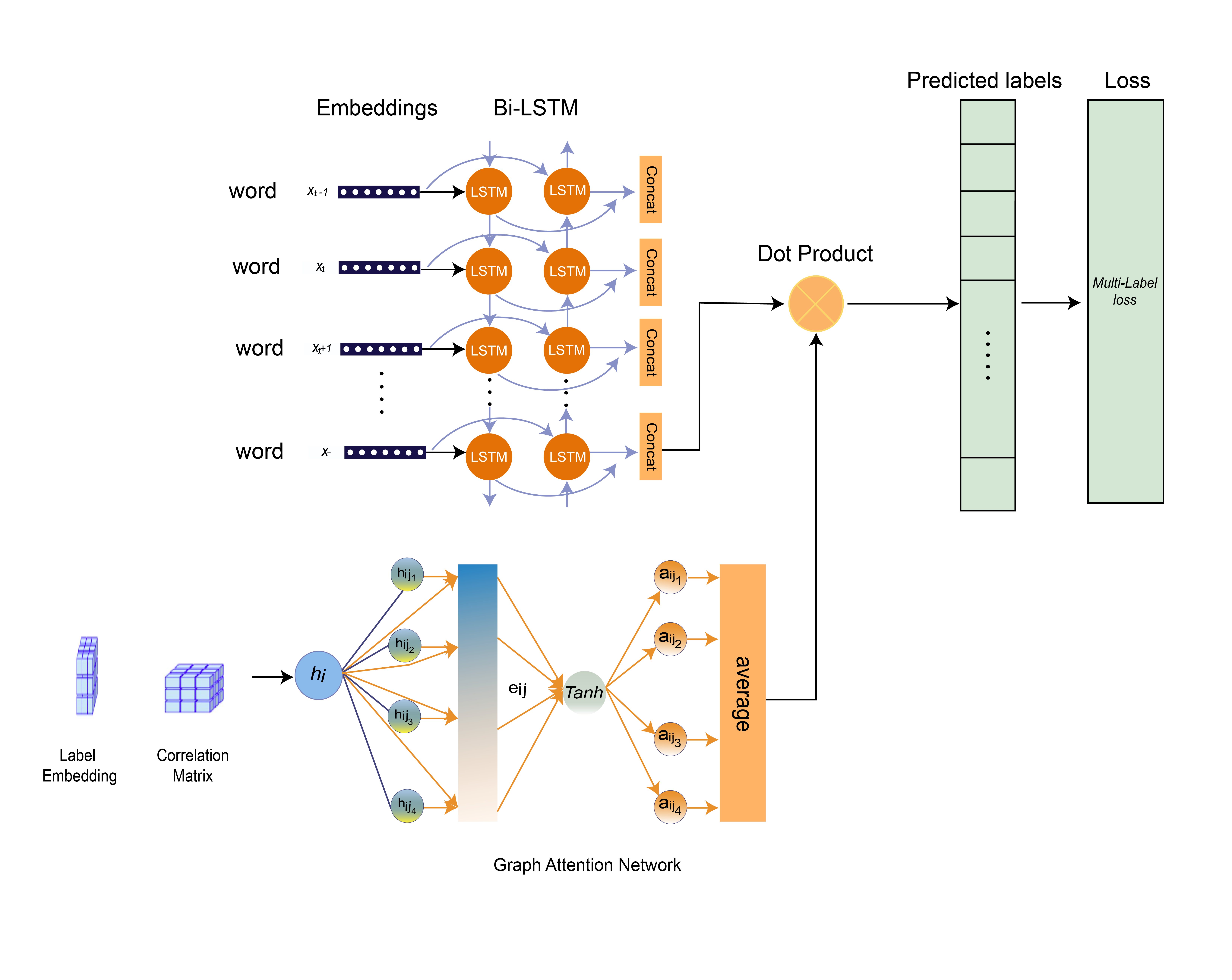
Figure 1: Illustration of overall structure of MAGNET model with a single Graph Attention layer for multi label text classification. $\left(x^{(n)},\mathbf{y}^{(n)}\right),n=1,2,\dots,N$ is input for BiLSTM to generate the feature vectors. $x_{(n)}$ are encoded using BERT embeddings. Input for Graph attention network is the Adjacency matrix $A\in\mathbb{R}{{}^{n\times n}}$ and label vectors $M\in\mathbb{R}{{}^{n\times d}}$. GAT output is attended label features which is applied on the feature vectors obtained from the BiLSTM

3.2 Node updating Mechanism in Graph convolution

In Graph Convolution Network Nodes can be updated by different types of node updating mechanisms. The basic version of GCN updates each node $i$ of the ${\ell}$-th layer, $\mathbf{H_{i}^{(\bm{\ell}+1)}}$, as follows.

$$\mathbf{H^{(\bm{\ell}+1)}=\sigma\left(AH^{\bm{\ell}}W^{\bm{\ell}}\right)}$$ (2)

Where $\sigma(\cdot)$ denote an activation function, $A$ is an adjacency matrix and $W^{({\ell})}$ is the convolution weights of the ${{\ell}}$-th layer. We represent each node of the graph structure as a label; at each layer, the label’s features are aggregated by neighbors to form the label features of the next layer. In this way, features become increasingly more abstract at each consecutive layer. e.g., label 2 has three adjacent labels 1, 3 and 4. In this case, another way to write equation (2) is

$$\mathbf{H_{2}^{(\bm{\ell}+1)}}=\mathbf{\sigma\Bigl{(}H_{2}^{(\bm{\ell})}W^{(\bm{\ell})}+H_{1}^{(\bm{\ell})}W^{(\bm{\ell})}}\\ \mathbf{+H_{3}^{(\bm{\ell})}W^{(\bm{\ell})}+H_{4}^{(\bm{\ell})}W^{(\bm{\ell})}\Bigr{)}}$$ (3)

So, in this case, the graph convolution network sums up all labels features with the same convolution weights, and then the result is passed through one activation function to produce the updated node feature output.

3.3 Graph Attention Networks for multi-label classification

In GCNs, the neighborhoods of nodes combine with equal or pre-defined weights. However, the influence of neighbors can vary greatly, and the attention mechanism can identify label importance in correlation graph by considering the importance of their neighbor labels.

The node updating mechanism, equation (3), can be written as a linear combination of neighboring labels with attention coefficients.

$$\mathbf{H_{2}^{(\bm{\ell}+1)}}=\mathbf{ReLU\Bigl{(}\alpha_{22}^{(\bm{\ell})}H_{2}^{(\bm{\ell})}W^{(\bm{\ell})}+\alpha_{21}^{(\bm{\ell})}H_{1}^{(\bm{\ell})}W^{(\bm{\ell})}}\\ \mathbf{+\alpha_{23}^{(\bm{\ell})}H_{3}^{(\bm{\ell})}W^{(\bm{\ell})}+\alpha_{24}^{(\bm{\ell})}H_{4}^{(\bm{\ell})}W^{(\bm{\ell})}\Bigr{)}}$$ (4)

where $\alpha_{ij}^{{\ell}}$ is an attention coefficient which measures the importance of the ${j}$th node in updating the ${i}$th node of the ${\ell}$-th hidden layer. The basic expression of the attention coefficient can be written as

$$\mathbf{\alpha_{ij}^{(\bm{\ell})}}=f\mathbf{\Big{(}H_{i}^{(\bm{\ell})}W^{(\bm{\ell})},H_{j}^{(\bm{\ell})}W^{(\bm{\ell})}\Big{)}}$$ (5)

The attention coefficient can be obtained typically by i) a similarity base, ii) concatenating features, and iii) coupling all features. We evaluate the attention coefficient by concatenating features.

$$\mathbf{\alpha_{ij}}=\mathbf{ReLU\left(\left(H_{i}W\right)\mathbin{\|}\left(H_{j}W\right)^{T}\right)}$$ (6)

In our experiment, we are using multi-head attention [Vaswani et al., 2017] that utilizes $K$ different heads to describe labels relationships. The operations of the layer are independently replicated $K$ times (each replication is done with different parameters), and the outputs are aggregated feature wise (typically by concatenating or adding).

$$\mathbf{H_{i}^{(\bm{\ell}+1)}}=Tanh\left(\frac{1}{K}\sum_{k=1}^{K}\sum_{j\in N(i)}\alpha_{ij,k}^{\bm{\ell}}H_{j}^{\bm{\ell}}W^{\bm{\ell}}\right)$$ (7)

Where $\alpha_{ij}$ is the attention coefficient of label $j$ to $i$. $N(i)$ represents the neighborhood of label $i$ in the graph. We use a cascade of GAT layers. For first layer the input is label embedding matrix $M\in\mathbb{R}{{}^{n\times d}}$.

$$\mathbf{H_{i}^{1}}=Tanh\left(\frac{1}{K}\sum_{k=1}^{K}\sum_{j\in N(i)}\alpha_{ij,k}^{(0)}MW^{(0)}\right)$$ (8)

The output from the previous GAT layer is fed into the successive GAT layer similar to RNN but the GAT layer weights are not shared

$$\mathbf{H_{i}^{(\bm{\ell}+1)}}=\underbrace{Tanh\left(\frac{1}{K}\sum_{k=1}^{K}\sum_{j\in N(i)}\alpha_{ij,k}^{\bm{\ell}}H_{i}^{\bm{\ell}}W^{\bm{\ell}}\right)}_{\text{attended label features}}$$ (9)

The output from the last layer is the attended label features $\mathbf{H_{gat}\in\mathbb{R}^{c\times d}}$ where $c$ denotes the number of labels and $d$ denotes the dimension of the attended label features. which is applied to the textual features from the BiLSTM.

3.4 Feature vector generation

We are using bidirectional LSTM (Hochreiter and Schmidhuber, 1997) to obtain the feature vectors. We use BERT for embedding the words and then feed it to BiLSTM for fine-tuning for the domain-specific task, BiLSTM reads the text sequence $x$ from both directions and computes the hidden states for each word,

$$\overrightarrow{\boldsymbol{h}}_{i}=\overrightarrow{\mathrm{LSTM}}\left(\overrightarrow{\boldsymbol{h}}_{i-1},\boldsymbol{x}_{i}\right)$$ (10)

$$\overleftarrow{\boldsymbol{h}}_{i}=\overleftarrow{\mathrm{LSTM}}\left(\overleftarrow{\boldsymbol{h}}_{i+1},\boldsymbol{x}_{i}\right)$$

We obtain the final hidden representation of the ${i}$-th word by concatenating the hidden states from both directions,

$$\boldsymbol{h}_{i}=\left[\overrightarrow{\boldsymbol{h}_{i}};\overleftarrow{\boldsymbol{h}}_{i}\right]$$ (11)

$$\mathbf{F=f_{rnn}(f_{BERT}(s;\theta_{BERT});\theta_{rnn})\in\mathbb{R}^{D}}$$ (12)

Where $s$ is the sentence, $\theta_{rnn}$ is Rnn parameters, $\theta_{BERT}$ is BERT’s parameter, $D$ is hidden size of BiLSTM. Later we multiply feature vectors with attended label features to get the final prediction score as,

$$\hat{\boldsymbol{y}}=\boldsymbol{F}\mathbf{\odot}\boldsymbol{H_{gat}}$$ (13)

Where $\mathbf{H_{gat}\in\mathbb{R}^{c\times d}}$ and $F$ is feature vectors obtained from BiLSTM model. Figure 1 shows the overall structure of the proposed model.

3.5 Adjacency matrix generation

In this section, we explain how to initialize the adjacency matrix for the GAT network. We use three different methods to initialize the weights..

• Identity Matrix We use the Identity matrix as the adjacency matrix. Ones on the main diagonal and zeros elsewhere, i.e., starting with zero correlation as a starting point.

• Xavier initialization We use Xavier initialization [Glorot and Bengio, 2010] to initialize the weight of adjacency matrix.

  $$\pm\frac{\sqrt{6}}{\sqrt{n_{i}+n_{i+1}}}$$ (14)

  where $n_{i}$ is the number of incoming network connections.

• Correlation matrix

  The correlation matrix is constructed by counting the pairwise co-occurrence of labels. The frequency vector is vector $F\in\mathbb{R}{{}^{n}}$ where $n$ is the number of labels and $F_{i}$ is the frequency of label $i$ in the overall training set. The co-occurrence matrix is then normalized by the frequency vector.

  A = M / F (15)

  where $M\in\mathbb{R}{{}^{n\times n}}$ is the co-occurrence matrix and $F\in\mathbb{R}{{}^{n}}$ is the frequency vector of individual labels. This is similar to how the correlation matrix built-in [Chen et al., 2019], except we do not employ binarization.

3.6 Loss function

We use Cross-entropy as the loss function. If the ground truth label of a data point is $y\in\mathbb{R}^{c}$ , where ${y}_{i}=\{0,1\}$

$$\mathbf{\mathcal{L}=\sum_{c=1}^{C}y^{c}\log\left(\sigma\left(\hat{y}^{c}\right)\right)+\left(1-y^{c}\right)\log\left(1-\sigma\left(\hat{y}^{c}\right)\right)}$$ (16)

Where $\sigma$ is sigmoid activation function

4 EXPERIMENT

In this section, we introduce the datasets, experiment details, and baseline results. Subsequently, the authors make a comparison of the proposed methods with baselines

4.1 Datasets

In this section, we provide detail and use the source of the datasets in the experiment. Table 2 shows the Statistics of all datasets.
Reuters-21578 is a collection of documents collected from Reuters News Wire in 1987. The Reuters-21578 test collection, together with its earlier variants, has been such a standard benchmark for the text categorization (TC) [Debole and Sebastiani, 2005]. It contains 10,788 documents, which has 8,630 documents for training and 2,158 for testing with a total of 90 categories.
RCV1-V2 provided by Lewis et al. (2004) [Lewis et al., 2004], consists of categorized newswire stories made available by Reuters Ltd. Each newswire story can have multiple topics assigned to it, with 103 topics in total. RCV1-V2 contains 8,04,414 documents which are divided into 6,43,531 documents for training and 1,60,883 for testing.
Arxiv Academic Paper Dataset (AAPD) is provided by Yang et al. (2018). The dataset consists of the abstract and its corresponding subjects of 55,840 academic papers, and each paper can have multiple subjects. The target is to predict subjects of an academic paper according to the content of the abstract. The AAPD dataset then divides into 44,672 documents for training and 11,168 for testing with a total of 54 classes.
Slashdot dataset was collected from the Slashdot website and consists of article blurbs labeled with the subject categories. Slashdot contains 19,258 samples for training and 4,814 samples for testing with a total of 291 classes.
Toxic comment dataset, We are using toxic comment dataset from Kaggle. This dataset has large number of comments from Wikipedia talk page edits. Human raters have labeled them for toxic behavior.

4.2 Experiment details

We implement our experiments in Tensorflow on an NVIDIA 1080Ti GPU. Our model consists of two GAT layers with multi-head attention. Table 1 shows the hyper-parameters of the model on five datasets. For label representations, we adopt 768 dim BERT trained on Wikipedia and BookCorpus. For the categories whose names contain multiple words, we obtain the label representation as to the average of embeddings for all words. For all datasets, the batch size is set to 250, and out of vocabulary(OOV) words are replaced with unk. We use BERT embedding to encode the sentences. We use Adam optimizer to minimize the final objective function. The learning rate is initialized to 0.001 and we make use of the dropout 0.5 (Srivastava et al. 2014) to avoid overfitting and clip the gradients (Pascanu, Mikolov, and Bengio 2013) to the maximum norm of 10.

Dataset	Vocab Size	Embed size	Hidden size	Attention heads
Reuters-21578	20,000	768	250	4
RCV1-V2	50,000	768	250	8
AAPD	30,000	768	250	8
Slashdot	30,000	768	300	4
Toxic Comment	50,000	768	200	8

Table 1: Main experimental hyper-parameters

4.3 Performance Evaluation

miF1 In the micro-average method, the individual true positives, false positives, and false negatives of the system are summed up for different sets and applied to get Micro-average F-Score.

$$F1-{Score_{micro}=\frac{\sum_{j=1}^{L}2tp_{j}}{\sum_{j=1}^{L}\left(2tp_{j}+fp_{j}+fn_{j}\right)}}$$ (17)

$${Precision_{micro}}=\frac{\sum_{j=1}^{L}tp_{j}}{\sum_{j=1}^{L}tp_{j}+fp_{j}}$$

$${Recall_{micro}=\frac{\sum_{j=1}^{L}tp_{j}}{\sum_{j=1}^{L}tp_{j}+fn_{j}}}$$

Hamming loss (HL): Hamming-Loss is the fraction of labels that are incorrectly predicted. [Destercke, 2014]. Therefore, hamming loss takes into account the prediction of both an incorrect label and a missing label normalized over the total number of classes and the total number of examples.

Dataset	Domain	#Train	#Test	Labels
Reuters-21578	Text	8,630	2,158	90
RCV1-V2	Text	6,43,531	1,60,883	103
AAPD	Text	44,672	11,168	54
Slashdot	Text	19,258	4,814	291
Toxic Comment	Text	126,856	31,714	7

Table 2: Statistics of the datasets

$$\textit{{HL}}=\frac{1}{|N|\cdot|L|}\sum_{i=1}^{|N|}\sum_{j=1}^{|L|}\operatorname{xor}\left(y_{i,j},z_{i,j}\right)$$ (18)

where $y_{i,j}$ is the target and $z_{i,j}$ is the prediction. Ideally, we would expect Hamming loss, ${HL=0}$, which would imply no error; practically the smaller the value of hamming loss, the better the performance of the learning algorithm.

4.4 Comparison of methods

We compare the performance of 27 algorithms, including state-of-the-art models. Furthermore, we compare the latest state-of-the-art models on the rcv1-v2 dataset. Compared algorithms can be categorized into three groups, as described below:

• Flat baselines Flat Baseline models transform the documents and extract the features using TF-IDF [Ramos,], later use those features as input to Logistic regression (LR) [Allison, 1999] , Support Vector Machine (SVM)[Hearst, 1998] , Hierarchical Support Vector Machine (HSVM) [Vural and Dy, 2004] , Binary Relevance (BR)[Boutell et al., 2004], Classifier Chains(CC)[Read et al., 2011]. Flat Baseline methods ignore the relation between words and dependency between labels.

• Sequence, Graph and N-gram based models

  These types of models first transform the text dataset into sequences of words, the graph of words or N-grams features, later apply different types of deep learning models on those features including CNN [Kim, 2014b], CNN-RNN [Chen et al., 2017], RCNN [Lai et al., 2015], DCNN [Schwenk et al., 2017], XML-CNN [Liu et al., 2017], HR-DGCNN [Peng et al., 2018], Hierarchical LSTM (HLSTM) [Chen et al., 2016], multi-label classification approach based on a conditional cyclic directed graphical model (CDN-SVM) [Guo and Gu, 2011], Hierarchical Attention Network (HAN) [Yang et al., 2016] and Bi-directional Block Self-Attention Network (Bi-BloSAN) [Shen et al., 2018] etc. for the multi-label classification task For example, Hierarchical Attention Networks for Document Classification (HAN) uses a GRU grating mechanism to encode the sequences and apply word and sentence level attention on those sequences for document classification. Bi-directional Block Self-Attention Network (BI-BloSAN) uses intra-block and inter-block self-attentions to capture both local and long-range context dependencies by splitting the sequences into several blocks.

• Recent state-of-the-art models

  We compare our model with different state-of-the-art models for multi-label classification task including BP-MLL_RAD [Nam et al., 2014], Input Encoding with Feature Message Passing (FMP) [Lanchantin et al., 2019], TEXT-CNN[Kim, 2014a], Hierarchical taxonomy-aware and attentional graph capsule recurrent CNNs framework (HE-AGCRCNN)[Peng et al., 2019], BOW-CNN[Johnson and Zhang, 2014], Capsule-B networks[Zhao et al., 2018], Hierarchical Text Classification with Reinforced Label Assignment (HiLAP)[Mao et al., 2019], Hierarchical Text Classification with Recursively Regularized Deep Graph-CNN (HR-DGCNN)[Peng et al., 2018], Hierarchical Transfer Learning-based Strategy (HTrans)[Banerjee et al., 2019], BERT (Bidirectional Encoder Representations from Transformers)[Devlin et al., 2019b], BERT-SGM[Yarullin and Serdyukov, 2019], For example FMP + LaMP is a variant of LaMP model which uses Input Encoding with Feature Message Passing (FMP). It achieves state-of-the-art accuracy across five metrics and seven datasets. HE-AGCRCNN uses a hierarchical taxonomy embedding method to learn the hierarchical relations among the labels.is another recent state-of-the-art model, which has shown outstanding performance in large-scale multi-label text classification. It uses a hierarchical taxonomy embedding method to learn the hierarchical relations among the labels. BERT (Bidirectional Encoder Representations from Transformers) is a recent pre-trained language model that has shown groundbreaking results in many NLP tasks. BERT uses attention mechanism (Transformer) to learns contextual relations between words in a text.

5 PERFORMANCE ANALYSIS

In this section, we will compare our proposed method with baselines on the test sets. Table 4 shows the detailed Comparisons of Micro F1-score for various state-of-the-art models.

5.1 Comparisons with State-of-the-art

First, we compare the result of Traditional Machine learning algorithms. Among LR, SVM, and HSVM, HSVM performs better than the other two. HSVM uses SVM at each node of the Decision tree. Later we compare the result of Hierarchical, CNN based models and graph-based deep learning models. Among Hierarchical Models HLSTM, HAN, HE-AGCRCNN, HR-DGCNN, HiLAP, and HTrans, HE-AGCRCNN performs better compared to other Hierarchical models. HAN and HLSTM methods are based on recurrent neural networks. While analyzing the performance of the recurrent model with baseline Flat models, recurrent neural networks perform worse than HSVM even though there was an ignorance of label dependency in baseline models. RNN faces the problem of vanishing gradients and exploding gradients when the sequences are too long. Graph model, HR-DGCNN, performs better than recurrent and baseline models. Comparing the CNN-based model RCNN, XML-CNN, DCNN, TEXTCNN, CNN, and CNN-RNN, TEXTCNN performs better among all of them while RCNN performs worse among them.

The sequence generator model treats the multi-label classification task as a sequence generation. When comparing the sequence generator models SGM-GE and seq2seq, SGM performs better than the seq2seq network. SGM utilizes the correlation between labels by using sequence generator model with a novel decoder structure.

Comparing the proposed MAGNET against the state-of-the-art models, MAGNET significantly improved previous state-of-the-art results, we see ~20$\%$ improvement in miF1 comparison to HSVM model. While comparing with the best Hierarchical text classification models, we observe ~11$\%$, ~19$\%$, ~5$\%$ and ~8$\%$ accuracy improvement compared to HE-AGCRCNN, HAN, HiLAP, HTrans respectively. The proposed model produced a ~16$\%$ improvement in miF1 over the popular bi-directional block self-attention network (Bi-BloSAN).

Comparing with CNN group models, proposed model improves the performance by ~12$\%$ and ~6$\%$ accuracy compared with TEXTCNN and BOW-CNN method respectively. MAGNET achieves ~2$\%$ improvement over state-of-the-art BERT model.

5.2 Evaluation on other datasets

We also evaluate our proposed model on four different datasets rather than RCV1 to observe the performance of the model on those datasets, which vary in the number of samples and the number of labels. Table 3 shows the miF1 scores for different datasets, and we also report the Hamming loss in Table 5. Evaluation results show that proposed methods achieve the best performance in the primary evaluation metrics. We observe  3$\%$ and 4$\%$ miF1 improvement in AAPD and Slashdot dataset, respectively, as compared to the CNN-RNN method.

F1-accuracy
Methods	Reuters-21578	AAPD	Slashdot	Toxic
BR	0.878	0.648	0.486	0.853
BR-support	0.872	0.682	0.516	0.874
CC	0.879	0.654	0.480	0.893
CNN	0.863	0.664	0.512	0.775
CNN-RNN	0.855	0.669	0.530	0.904
MAGNET	0.899	0.696	0.568	0.930

Table 3: Comparisons of Micro F1-score for various models on four benchmark datasets.

5.3 Analysis and Discussion

Here we discuss a further analysis of the model and experimental results. We report the evaluation results in terms of hamming loss and macro-F1 score. We are using a moving average with a window size of 3 to draw the plots to make the scenarios more comfortable to read.

5.3.1 Impact of initialization of the adjacency matrix

We initialized the adjacency matrix in three different ways random, identity, and co-occurrence matrix. We hypothesized that the co-occurrence matrix would perform the best since the model is fed with richer prior information than the identity matrix, where the correlation is zero and random matrix. To our surprise, random initialization performed the best at 0.887, and identity matrix performed the worst at 0.865, whereas the co-occurrence matrix achieved the micro-F1 score of 0.878. Even though Xavier initializer performed the best, all the other random initializers performed better than co-occurrence and identity matrices. This shows that the textual information from samples contain richer information than that in the label co-occurrence matrix that we initialize the adjacency with, and both co-occurrence and identity matrix, traps the model in a local minima.

Rcv1-v2
Method	Accuracy
LR	0.692
SVM	0.691
HSVM	0.693
HLSTM	0.673
RCNN	0.686
XML-CNN	0.695
HAN	0.696
Bi-BloSAN	0.72
DCNN	0.732
SGM+GE	0.719
CAPSULE-B	0.739
CDN-SVM	0.738
HR-DGCNN	0.761
TEXTCNN	0.766
HE-AGCRCNN	0.778
BP-MLLRAD	0.780
HTrans	0.805
BOW-CNN	0.827
HilAP	0.833
BERT	0.864
BERT + SGM	0.846
FMP + LaMPpr	0.877
MAGNET	0.885

Table 4: Comparisons of Micro F1-score for various state-of-the-art models on Rcv1-v2 dataset.

Hamming-loss
Methods	Rcv1-v2	AAPD	Reuters-21578	Slashdot	Toxic
BR	0.0093	0.0316	0.0032	0.052	0.034
CC	0.0089	0.0306	0.0031	0.057	0.030
CNN	0.0084	0.0287	0.0033	0.049	0.039
CNN-RNN	0.0086	0.0282	0.0037	0.046	0.025
MAGNET	0.0079	0.0252	0.0029	0.039	0.022

Table 5: Comparisons of hamming loss for various models on four benchmark datasets.
the smaller the value, the better.

5.3.2 Results on different types of word embeddings

In this section, we investigate the impact of the four different word embeddings on our proposed architecture, namely the Word2Vec embeddings[Mikolov et al., 2013], Glove embeddings [Pennington et al., 2014], Random embeddings, BERT embeddings [Devlin et al., 2019a]. Figure (2) and Figure (3) shows the f1 score of all four different word embeddings on the (unseen) test dataset of Reuters-21578.

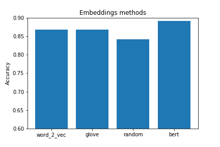
Figure 2: Different types of word embeddings performance on MAGNET x axis refer to the different types of word embeddings and y axis refer to the Accuracy ( F1-score)

Accordingly, we make the following observations:

• Glove and word2vec embeddings produce similaer results.

• Random embeddings perform worse than other embeddings. Pre-trained word embeddings have proven to be highly useful in our proposed architecture compared to the random embeddings.

• BERT embeddings outperform other embeddings in this experiment. Therefore, using BERT feature embeddings increase the accuracy and performance of our architecture.

Our proposed model uses BERT embeddings for encoding the sentences.

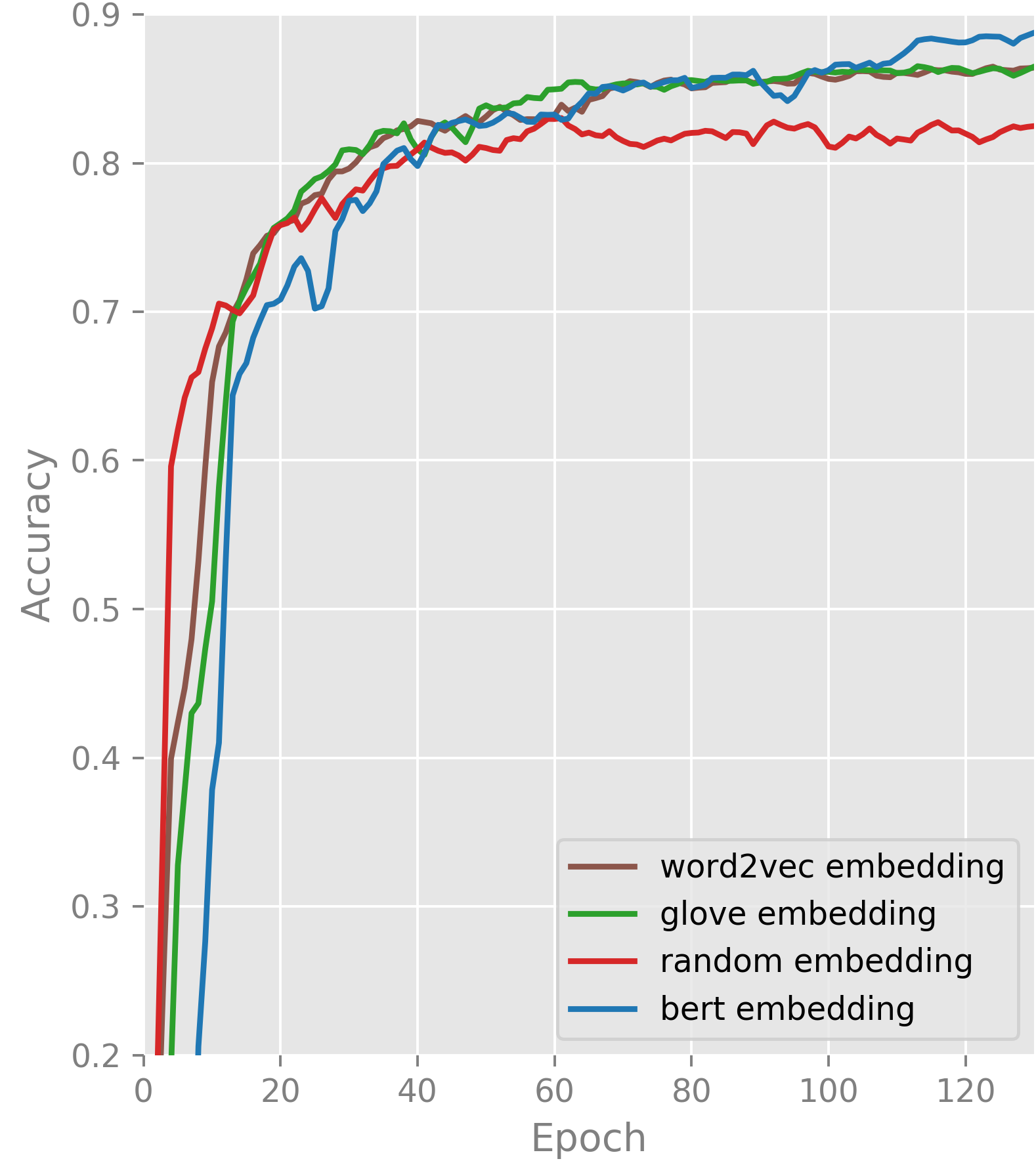
Figure 3: Performance of proposed model on different types of word embeddings. x-axis is the number of epoch and the y-axis refers to the micro-F1 score.

5.3.3 Comparison between Two different Graph neural networks

In this section, we compare the performance of GAT and GCN networks. The critical difference between GAT and GCN is how the information aggregates from the neighborhood. GAT computes the hidden states of each node by attending over its neighbors, following a self-attention strategy where GCN produces the normalized sum of the node features of neighbors.

GAT improved the average miF1 score by 4$\%$ over the GCN model. It shows that the GAT model captures better label correlation compare to GCN. The attention mechanism can identify label importance in correlation graph by considering the significance of their neighbor labels.

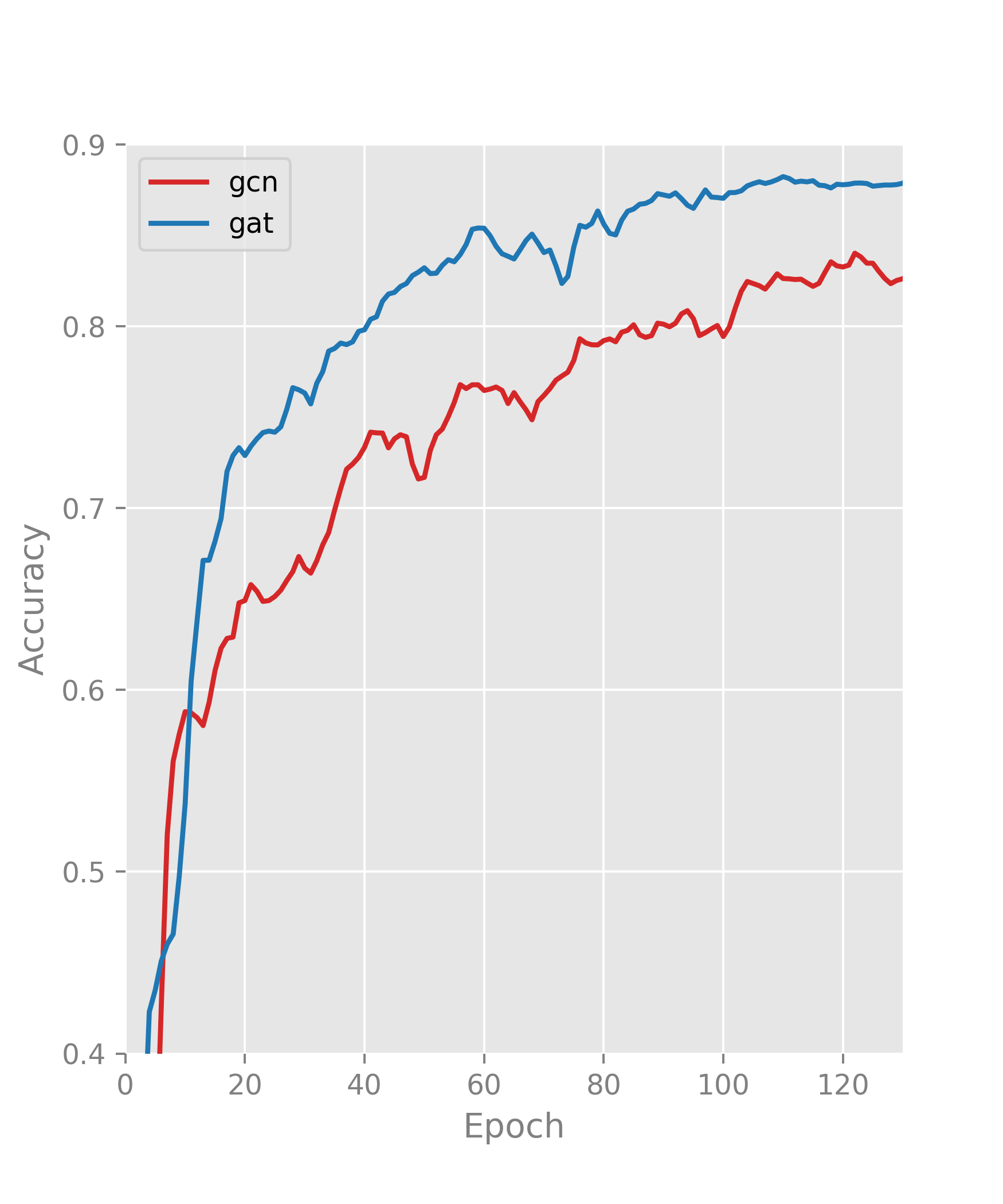
Figure 4: Performance of GAT vs GCN. x-axis is number of epochs and y-axis is micro-F1 score.

Figure (4) shows the accuracy of both neural network on Reuters-21578 dataset.

5.4 Conclusion

The proposed approach can improve the accuracy and efficiency of models and can work across a wide range of data types and applications. To model and capture the correlation between labels, we proposed a GAT based model for multi-label text classification.

We evaluated the proposed model on various datasets and presented the results. The combination of GAT with bi-directional LSTM shows that it has achieved consistently higher accuracy than those obtained by conventional approaches.

Even though our proposed model performs very well, there are still some limitations. When the dataset contains a large number of labels correlation matrix will be very large, and training the model can be difficult. Our work alleviates this problem to some extent, but we still think the exploration of more effective solutions is vital in the future.

REFERENCES

- Allison, 1999 Allison, P. (1999). Logistic Regression Using Sas®: Theory and Application. SAS Publishing, first edition.
- Banerjee et al., 2019 Banerjee, S., Akkaya, C., Perez-Sorrosal, F., and Tsioutsiouliklis, K. (2019). Hierarchical transfer learning for multi-label text classification. In Proceedings of the 57th Conference of the Association for Computational Linguistics, ACL 2019, Florence, Italy, July 28- August 2, 2019, Volume 1: Long Papers, pages 6295–6300.
- Boutell et al., 2004 Boutell, M. R., Luo, J., Shen, X., and Brown, C. M. (2004). Learning multi-label scene classification. Pattern Recognition, 37(9):1757 – 1771.
- Cai et al., 2017 Cai, H., Zheng, V. W., and Chang, K. C. (2017). A comprehensive survey of graph embedding: Problems, techniques and applications. CoRR, abs/1709.07604.
- Chen et al., 2017 Chen, G., Ye, D., Xing, Z., Chen, J., and Cambria, E. (2017). Ensemble application of convolutional and recurrent neural networks for multi-label text categorization. In 2017 International Joint Conference on Neural Networks (IJCNN), pages 2377–2383.
- Chen et al., 2016 Chen, H., Sun, M., Tu, C., Lin, Y., and Liu, Z. (2016). Neural sentiment classification with user and product attention. In Proceedings of the 2016 Conference on Empirical Methods in Natural Language Processing, EMNLP 2016, Austin, Texas, USA, November 1-4, 2016, pages 1650–1659.
- Chen et al., 2019 Chen, Z.-M., Wei, X.-S., Wang, P., and Guo, Y. (2019). Multi-Label Image Recognition with Graph Convolutional Networks. In The IEEE Conference on Computer Vision and Pattern Recognition (CVPR).
- Debole and Sebastiani, 2005 Debole, F. and Sebastiani, F. (2005). An analysis of the relative hardness of reuters-21578 subsets: Research articles. J. Am. Soc. Inf. Sci. Technol., 56(6):584–596.
- Destercke, 2014 Destercke, S. (2014). Multilabel prediction with probability sets: The hamming loss case. In Information Processing and Management of Uncertainty in Knowledge-Based Systems - 15th International Conference, IPMU 2014, Montpellier, France, July 15-19, 2014, Proceedings, Part II, pages 496–505.
- Devlin et al., 2019a Devlin, J., Chang, M., Lee, K., and Toutanova, K. (2019a). BERT: pre-training of deep bidirectional transformers for language understanding. In Proceedings of the 2019 Conference of the North American Chapter of the Association for Computational Linguistics: Human Language Technologies, NAACL-HLT 2019, Minneapolis, MN, USA, June 2-7, 2019, Volume 1 (Long and Short Papers), pages 4171–4186.
- Devlin et al., 2019b Devlin, J., Chang, M.-W., Lee, K., and Toutanova, K. (2019b). Bert: Pre-training of deep bidirectional transformers for language understanding. In NAACL-HLT.
- Fout et al., 2017 Fout, A., Byrd, J., Shariat, B., and Ben-Hur, A. (2017). Protein interface prediction using graph convolutional networks. In Proceedings of the 31st International Conference on Neural Information Processing Systems, NIPS’17, pages 6533–6542, USA. Curran Associates Inc.
- Glorot and Bengio, 2010 Glorot, X. and Bengio, Y. (2010). Understanding the difficulty of training deep feedforward neural networks. In Proceedings of the Thirteenth International Conference on Artificial Intelligence and Statistics, AISTATS 2010, Chia Laguna Resort, Sardinia, Italy, May 13-15, 2010, pages 249–256.
- Gopal and Yang, 2010 Gopal, S. and Yang, Y. (2010). Multilabel classification with meta-level features. pages 315–322.
- Gopal and Yang, 2015 Gopal, S. and Yang, Y. (2015). Hierarchical bayesian inference and recursive regularization for large-scale classification. TKDD, 9(3):18:1–18:23.
- Gopal et al., 2012 Gopal, S., Yang, Y., Bai, B., and Niculescu-Mizil, A. (2012). Bayesian models for large-scale hierarchical classification. In Advances in Neural Information Processing Systems 25: 26th Annual Conference on Neural Information Processing Systems 2012. Proceedings of a meeting held December 3-6, 2012, Lake Tahoe, Nevada, United States, pages 2420–2428.
- Guo and Gu, 2011 Guo, Y. and Gu, S. (2011). Multi-label classification using conditional dependency networks. In IJCAI 2011, Proceedings of the 22nd International Joint Conference on Artificial Intelligence, Barcelona, Catalonia, Spain, July 16-22, 2011, pages 1300–1305.
- Hearst, 1998 Hearst, M. A. (1998). Support vector machines. IEEE Intelligent Systems, 13(4):18–28.
- Johnson and Zhang, 2014 Johnson, R. and Zhang, T. (2014). Effective use of word order for text categorization with convolutional neural networks. CoRR, abs/1412.1058.
- Katakis et al., 2008 Katakis, I., Tsoumakas, G., and Vlahavas, I. (2008). Multilabel text classification for automated tag suggestion. In Proceedings of the ECML/PKDD 2008 Discovery Challenge.
- Kim, 2014a Kim, Y. (2014a). Convolutional neural networks for sentence classification. In Proceedings of the 2014 Conference on Empirical Methods in Natural Language Processing, EMNLP 2014, October 25-29, 2014, Doha, Qatar, A meeting of SIGDAT, a Special Interest Group of the ACL, pages 1746–1751.
- Kim, 2014b Kim, Y. (2014b). Convolutional neural networks for sentence classification. CoRR, abs/1408.5882.
- Kipf and Welling, 2016 Kipf, T. N. and Welling, M. (2016). Semi-supervised classification with graph convolutional networks. CoRR, abs/1609.02907.
- Lai et al., 2015 Lai, S., Xu, L., Liu, K., and Zhao, J. (2015). Recurrent convolutional neural networks for text classification. In Proceedings of the Twenty-Ninth AAAI Conference on Artificial Intelligence, January 25-30, 2015, Austin, Texas, USA, pages 2267–2273.
- Lanchantin et al., 2019 Lanchantin, J., Sekhon, A., and Qi, Y. (2019). Neural message passing for multi-label classification. CoRR, abs/1904.08049.
- Lewis et al., 2004 Lewis, D. D., Yang, Y., Rose, T. G., and Li, F. (2004). Rcv1: A new benchmark collection for text categorization research. J. Mach. Learn. Res., 5:361–397.
- Liu et al., 2017 Liu, J., Chang, W., Wu, Y., and Yang, Y. (2017). Deep learning for extreme multi-label text classification. In Proceedings of the 40th International ACM SIGIR Conference on Research and Development in Information Retrieval, Shinjuku, Tokyo, Japan, August 7-11, 2017, pages 115–124.
- Luaces et al., 2012 Luaces, O., Díez, J., Barranquero, J., del Coz, J. J., and Bahamonde, A. (2012). Binary relevance efficacy for multilabel classification. Progress in Artificial Intelligence, 1(4):303–313.
- Mao et al., 2019 Mao, Y., Tian, J., Han, J., and Ren, X. (2019). Hierarchical text classification with reinforced label assignment. CoRR, abs/1908.10419.
- Mikolov et al., 2013 Mikolov, T., Sutskever, I., Chen, K., Corrado, G. S., and Dean, J. (2013). Distributed representations of words and phrases and their compositionality. In Advances in Neural Information Processing Systems 26: 27th Annual Conference on Neural Information Processing Systems 2013. Proceedings of a meeting held December 5-8, 2013, Lake Tahoe, Nevada, United States., pages 3111–3119.
- Nam et al., 2014 Nam, J., Kim, J., Loza Menc’ia, E., Gurevych, I., and Fürnkranz, J. (2014). Large-scale multi-label text classification - revisiting neural networks. In Machine Learning and Knowledge Discovery in Databases - European Conference, ECML PKDD 2014, Nancy, France, September 15-19, 2014. Proceedings, Part II, pages 437–452.
- Peng et al., 2019 Peng, H., Li, J., Gong, Q., Wang, S., He, L., Li, B., Wang, L., and Yu, P. S. (2019). Hierarchical taxonomy-aware and attentional graph capsule rcnns for large-scale multi-label text classification. CoRR, abs/1906.04898.
- Peng et al., 2018 Peng, H., Li, J., He, Y., Liu, Y., Bao, M., Wang, L., Song, Y., and Yang, Q. (2018). Large-scale hierarchical text classification with recursively regularized deep graph-cnn. In Proceedings of the 2018 World Wide Web Conference on World Wide Web, WWW 2018, Lyon, France, April 23-27, 2018, pages 1063–1072.
- Pennington et al., 2014 Pennington, J., Socher, R., and Manning, C. D. (2014). Glove: Global vectors for word representation. In Proceedings of the 2014 Conference on Empirical Methods in Natural Language Processing, EMNLP 2014, October 25-29, 2014, Doha, Qatar, A meeting of SIGDAT, a Special Interest Group of the ACL, pages 1532–1543.
- Quinlan, 1993 Quinlan, J. R. (1993). C4.5: Programs for Machine Learning. Morgan Kaufmann Publishers Inc., San Francisco, CA, USA.
- Ramos, Ramos, J. Using tf-idf to determine word relevance in document queries.
- Read et al., 2011 Read, J., Pfahringer, B., Holmes, G., and Frank, E. (2011). Classifier chains for multi-label classification. Machine Learning, 85(3):333–359.
- Schapire and Singer, 2000 Schapire, R. E. and Singer, Y. (2000). Boostexter: A boosting-based system for text categorization. Machine Learning, 39(2/3):135–168.
- Schwenk et al., 2017 Schwenk, H., Barrault, L., Conneau, A., and LeCun, Y. (2017). Very deep convolutional networks for text classification. In Proceedings of the 15th Conference of the European Chapter of the Association for Computational Linguistics, EACL 2017, Valencia, Spain, April 3-7, 2017, Volume 1: Long Papers, pages 1107–1116.
- Shen et al., 2018 Shen, T., Zhou, T., Long, G., Jiang, J., and Zhang, C. (2018). Bi-directional block self-attention for fast and memory-efficient sequence modeling. CoRR, abs/1804.00857.
- Sun and Lim, 2001 Sun, A. and Lim, E. (2001). Hierarchical text classification and evaluation. In Proceedings of the 2001 IEEE International Conference on Data Mining, 29 November - 2 December 2001, San Jose, California, USA, pages 521–528.
- Vaswani et al., 2017 Vaswani, A., Shazeer, N., Parmar, N., Uszkoreit, J., Jones, L., Gomez, A. N., Kaiser, L., and Polosukhin, I. (2017). Attention is all you need. CoRR, abs/1706.03762.
- Velickovic et al., 2018 Velickovic, P., Cucurull, G., Casanova, A., Romero, A., Liò, P., and Bengio, Y. (2018). Graph attention networks. In 6th International Conference on Learning Representations, ICLR 2018, Vancouver, BC, Canada, April 30 - May 3, 2018, Conference Track Proceedings.
- Vural and Dy, 2004 Vural, V. and Dy, J. G. (2004). A hierarchical method for multi-class support vector machines. In Proceedings of the Twenty-first International Conference on Machine Learning, ICML ’04, pages 105–, New York, NY, USA. ACM.
- Wu et al., 2019 Wu, Z., Pan, S., Chen, F., Long, G., Zhang, C., and Yu, P. S. (2019). A comprehensive survey on graph neural networks. CoRR, abs/1901.00596.
- Xiao et al., 2011 Xiao, L., Zhou, D., and Wu, M. (2011). Hierarchical classification via orthogonal transfer. In Proceedings of the 28th International Conference on Machine Learning, ICML 2011, Bellevue, Washington, USA, June 28 - July 2, 2011, pages 801–808.
- Xue et al., 2008 Xue, G., Xing, D., Yang, Q., and Yu, Y. (2008). Deep classification in large-scale text hierarchies. In Proceedings of the 31st Annual International ACM SIGIR Conference on Research and Development in Information Retrieval, SIGIR 2008, Singapore, July 20-24, 2008, pages 619–626.
- Yang et al., 2016 Yang, Z., Yang, D., Dyer, C., He, X., Smola, A. J., and Hovy, E. H. (2016). Hierarchical attention networks for document classification. In NAACL HLT 2016, The 2016 Conference of the North American Chapter of the Association for Computational Linguistics: Human Language Technologies, San Diego California, USA, June 12-17, 2016, pages 1480–1489.
- Yarullin and Serdyukov, 2019 Yarullin, R. and Serdyukov, P. (2019). Bert for sequence-to-sequence multi-label text classification.
- Ying et al., 2018 Ying, R., He, R., Chen, K., Eksombatchai, P., Hamilton, W. L., and Leskovec, J. (2018). Graph convolutional neural networks for web-scale recommender systems. CoRR, abs/1806.01973.
- Zhang et al., 2018 Zhang, M.-L., Li, Y.-K., Liu, X.-Y., and Geng, X. (2018). Binary relevance for multi-label learning: an overview. Frontiers of Computer Science, 12(2):191–202.
- Zhao et al., 2018 Zhao, W., Ye, J., Yang, M., Lei, Z., Zhang, S., and Zhao, Z. (2018). Investigating capsule networks with dynamic routing for text classification. CoRR, abs/1804.00538.