Abstract

In this work, we focus on the use of influence functions to identify relevant training examples that one might hope “explain” the predictions of a machine learning model. One shortcoming of influence functions is that the training examples deemed most “influential” are often outliers or mislabelled, making them poor choices for explanation. In order to address this shortcoming, we separate the role of global versus local influence. We introduce RelatIF, a new class of criteria for choosing relevant training examples by way of an optimization objective that places a constraint on global influence. RelatIF considers the local influence that an explanatory example has on a prediction relative to its global effects on the model. In empirical evaluations, we find that the examples returned by RelatIF are more intuitive when compared to those found using influence functions.

1 Introduction

As the use of black-box models becomes widespread, many believe that their predictions must be accompanied by interpretable explanations (Lipton, 2016; Doshi-Velez & Kim, 2017; Goodman & Flaxman, 2017). There is a growing body of research concerned with how to best explain black-box predictions  (Kim et al., 2017; Ribeiro et al., 2018; Lundberg & Lee, 2017). A natural way to explain a model prediction is to provide supporting examples from the training data. However, one must choose which examples are most relevant. One approach is to trace the model prediction back to the training examples and determine the impact of each individual training example. This idea underlies so-called influence functions (IF), which quantify the impact of an individual example on a prediction in a differentiable model (Jaeckel, 1972; Hampel, 1974). The use of IF to explain black-box predictions by training examples with high influence was pioneered by Koh & Liang (2017).

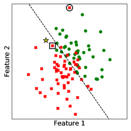
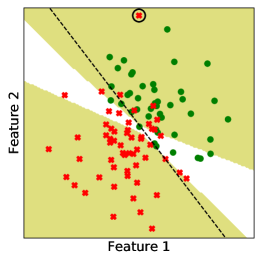
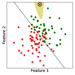
(a)		(b)	(c)

Figure 1: Binary classification by linear decision boundaries (dashed line) to illustrate the difference between IF and RelatIF. (a) The model makes a prediction for the test input (star). As estimated by IF, the most influential training example for the prediction is an outlier (circled). Using RelatIF, the most influential training example is more typical (encased in a square). (b) Using IF, every test input falling within the shaded yellow region is most influenced by the same outlier (circled). Test inputs in the remaining white region are most influenced by one of 5 other high loss examples. (c) Using RelatIF, the region where test inputs are most influenced by the outlier (circled) shrinks. Test inputs in the remaining region are most influenced by one of 65 other examples.

In this work, we revisit the use of IF for identifying examples to explain predictions. Our motivation is the observation that the most influential training examples returned by IF are often mislabelled or outliers, on the account of these examples also incurring high loss (see Fig. 1(a)). This phenomenon is well documented in the literature (Hampel, 1974; Campbell, 1978; Cook & Weisberg, 1982; Croux & Haesbroeck, 2000). As a result, we find that the set of examples deemed “influential” tend to be highly overlapping, in the sense that the predictions for many different inputs are all most affected by the same small set of training examples. In other words, these training examples seem to have a global impact on the model. Fig. 1 (b) illustrates these effects. Returning examples from an overlapping set of high loss training examples may be desirable when the recipient of the explanation is attempting to debug or otherwise improve the model. However, these examples can be unsatisfying as an explanation for an end user. Explaining a prediction by returning high loss training examples, which are often unusual or misclassified, does not inspire confidence in the model. Nor does it inspire confidence when, for several seemingly different inputs, the same high-loss examples are returned as an explanation.

We propose RelatIF, a new class of criteria for identifying “relevant” training examples to explain a prediction. RelatIF considers the local influence that an explanatory example has on a prediction relative to its global effects on the model. We formulate these criteria in terms of a constrained optimization problem: for a given allowable global “impact” on the model, which training examples most influence the specific prediction? We argue that this approach is better suited to producing an explanatory training example for an end user. Fig. 1(c) illustrates how this objective dampens the influence of an outlier. We show experimentally that RelatIF returns training examples that are more typical as well as more specific to a given input when compared to those identified using IF.

2 Preliminaries

Consider a family of predictors, indexed by parameter values $\theta\in\mathbb{R}^{d}$, each a map taking input values $x\in\mathcal{X}$ to target values $y\in\mathcal{Y}$. Let $S=(z_{1},z_{2},\ldots,z_{n})$ denote the training examples, where $z_{i}=(x_{i},y_{i})\in\mathcal{X}\times\mathcal{Y}$ is a pair of an input and target. Let $\ell(z,\theta)$ be the loss for a point $z$ under model parameters $\theta$. Our focus is on algorithms, like stochastic gradient descent (SGD), that return some first-order stationary point $\theta(w_{1},\dots,w_{n})$ of the objective

$$\sum_{i=1}^{n}w_{i}\ell(z_{i},\theta),$$ (1)

i.e., we are studying the parameters learned by weighted empirical risk minimization, where each $w_{i}$ is the weight given to the training example $z_{i}$. We are primarily interested in the parameter $\theta^{*}=\theta(1/n,\dots,1/n)$ obtained by weighting all points equally. Given an unseen input $x$, our goal is to identify training examples $z_{i}$ that, through training, had a “meaningful” influence on the prediction that $\theta^{*}$ renders for $x$.

A simple way to measure the effect of each example $z_{i}$ on training is to re-weight its contribution, retrain from scratch, and evaluate the change to the learned parameters. To that end, let $\theta^{*}_{i,\epsilon_{i}}=\theta(1/n,\dots,1/n+\epsilon_{i},\dots,1/n)$, where only the $i$’th weight is modified to be $w_{i}=\frac{1}{n}+\epsilon$. Any deviations of $w_{i}$ from $\frac{1}{n}$ is denoted by $\epsilon_{i}$, i.e., $\epsilon_{i}=w_{i}-\frac{1}{n}$. Taking $\epsilon_{i}=-\frac{1}{n}$, equivalently, setting $w_{i}=0$, constitutes dropping an example from the training set.

Exhaustive retraining, however, is computationally prohibitive. Instead, we will make an infinitesimal analysis, as was pioneered in the development of influence functions (Hampel, 1974; Jaeckel, 1972). To do so, we will assume that the parameter $\theta(w_{1},\dots,w_{n})$ is a differentiable function of the weights at $w_{1}=\dotsm=w_{n}=\frac{1}{n}$. Further, we will assume that $\ell(z,\theta)$ is strictly convex, and twice continuously differentiable, in $\theta$.

The method of influence functions (IF) allows us to approximate how (some function of) the learned parameters $\theta^{*}$ would change if we were to reweight a training example $z_{i}$. The key idea is to make a first-order approximation of change in $\theta^{*}$ around $\epsilon_{i}=0$. The same method can be extended to approximate changes in any twice continuously differentiable functions $f$ of the parameters around $\epsilon_{i}=0$. Namely, one can approximate how some $f(\theta^{*}_{i,\epsilon_{i}})$ changes with $\epsilon_{i}$ by considering $\mathrm{d}f(\theta^{*}_{i,\epsilon_{i}})/\mathrm{d}\epsilon_{i}\rvert_{\epsilon_{i}=0}$ . Indeed, our primary interest is the influence on the loss for a test sample.

Definition 2.1.

Fix a test sample $z_{\text{test}}=(x_{\text{test}},y_{\text{test}})$. The influence of $z_{i}$ on (the loss of) $z_{\text{test}}$ is defined to be

$$\mathcal{I}_{\text{test},i}=-\frac{\mathrm{d}\ell(z_{\text{test}},\theta^{*}_{i,\epsilon_{i}})}{\mathrm{d}\epsilon_{i}}\bigg{\rvert}_{\epsilon_{i}=0}=-g^{T}_{\text{test}}\frac{\mathrm{d}\theta^{*}_{i,\epsilon_{i}}}{\mathrm{d}\epsilon_{i}}\bigg{\rvert}_{\epsilon_{i}=0},$$

where $g_{\text{test}}=\nabla_{\theta^{*}}\ell(z_{\text{test}},\theta^{*})$.

Note that the second equality follows from the chain rule and that $\theta^{*}_{i,\epsilon_{i}}\rvert_{\epsilon_{i}=0}=\theta^{*}$.

Because we consider a negative change in Definition 2.1, a training example $z_{i}$ having positive influence on $z_{\text{test}}$ decreases the loss $\ell(z_{\text{test}},\theta^{*}_{i,\epsilon_{i}})$ when upweighted and may thus be considered helpful. A training example having negative influence on $z_{\text{test}}$ increases the loss and may thus be considered harmful.

2.1 Influence for General Loss Functions

Under certain conditions, it can be shown that

$$\frac{\mathrm{d}\theta^{*}_{i,\epsilon_{i}}}{\mathrm{d}\epsilon_{i}}\bigg{\rvert}_{\epsilon_{i}=0}=-H_{\theta^{*}}^{-1}g_{i},$$ (2)

where $H_{\theta^{*}}=\frac{1}{n}\sum_{i}\nabla^{2}_{\theta^{*}}\ell(z_{i},\theta^{*})$ is the Hessian of the objective at $\theta^{*}$ and $g_{i}=\nabla_{\theta^{*}}\ell(z_{i},\theta^{*})$. This result can be obtained by applying the implicit function theorem to the first-order optimality conditions for Eq. 1 (Cook & Weisberg, 1982). In this case, the expression for the influence of $z_{i}$ on $z_{\text{test}}$ becomes

$$\mathcal{I}_{\text{test},i}=g_{\text{test}}^{T}H^{-1}_{\theta^{*}}g_{i}.$$ (3)

Again noting that $\theta^{*}_{i,\epsilon_{i}}\rvert_{\epsilon_{i}=0}=\theta^{*}$, we can form a first-order Taylor series approximation for the change in model parameters due to upweighting $z_{i}$,

$$\theta^{*}_{i,\epsilon_{i}}-\theta^{*}\approx\frac{\mathrm{d}\theta^{*}_{i,\epsilon_{i}}}{\mathrm{d}\epsilon_{i}}\bigg{\rvert}_{\epsilon_{i}=0}\epsilon_{i}=-H_{\theta^{*}}^{-1}g_{i}\epsilon_{i}.$$ (4)

Similarly, we can approximate the change in loss via

$$\ell(z_{\text{test}},\theta^{*}_{i,\epsilon_{i}})-\ell(z_{\text{test}},\theta^{*}) \approx\frac{\mathrm{d}\ell(z_{\text{test}},\theta^{*}_{i,\epsilon_{i}})}{\mathrm{d}\epsilon_{i}}\epsilon_{i}$$

$$=-g_{\text{test}}^{T}H^{-1}_{\theta^{*}}g_{i}\epsilon_{i}.$$ (5)

for an infinitesimal change $\epsilon$ in $w_{i}$. The last equation follows from Eq. 4.

2.2 Influence in Maximum Likelihood

We have presented influence functions as they have been derived for the analysis of a broad class of empirical risk minimization objectives. In this section, we study the special case of cross entropy loss and maximum likelihood estimation (MLE), which leads us to an alternative representation of IF in terms of Fisher information. We use this formulation of IF to derive relative influence in Section 3.

Let $p_{\theta}(y|x)$ be a parametric statistical model (i.e., likelihood) and let $\ell((x,y),\theta)=-\log p_{\theta}(y|x)$. Global optimization of Eq. 1 corresponds to maximum likelihood estimation. As shown in Ting & Brochu (2018), in this setting the influence function satisfies

$$\mathcal{I}_{\text{test},i}=g_{\text{test}}^{T}F^{-1}_{\theta^{*}}g_{i},$$ (6)

where

$$F_{\theta}=\frac{1}{n}\sum_{i=1}^{n}\mathbb{E}_{p_{\theta}}\nabla_{\theta}\log p_{\theta}(y|x_{i})\nabla_{\theta}\log p_{\theta}(y|x_{i})^{T}$$ (7)

is the Fisher information matrix. Then a Taylor series approximation yields

$$\theta^{*}_{i,\epsilon_{i}}-\theta^{*} \approx-F^{-1}_{\theta^{*}}g_{i}\epsilon_{i},\text{~{}~{}and}$$ (8)

$$\ell(z_{\text{test}},\theta^{*}_{i,\epsilon_{i}})-\ell(z_{\text{test}},\theta^{*}) \approx-g_{\text{test}}^{T}F^{-1}_{\theta^{*}}g_{i}\epsilon_{i}.$$ (9)

We briefly discuss the relationship between $F_{\theta^{*}}$ and $H_{\theta^{*}}$ in Appendix A. For a more thorough treatment, see (Martens, 2014).

3 Relative Influence

For a given test input $x_{\text{test}}$, we would like to identify the training examples that serve to explain the target $y_{\text{test}}$. The change in loss on $z_{\text{test}}=(x_{\text{test}},y_{\text{test}})$ due to re-weighting each $z_{i}$ in $S$ is described by $\{\mathcal{I}_{\text{test},i}\}_{i=1,...,n}$. Returning the top-k examples that maximize $\lvert\mathcal{I}_{\text{test},i}\rvert$ constitutes one form of explanation. However, top influential examples selected via influence functions are often high-loss, i.e., they are either mislabelled, outliers, or otherwise atypical. The sets of top-k examples which maximize $\lvert\mathcal{I}_{\text{test},i}\rvert$ for different test inputs also often overlap. We hypothesize that these types of examples are returned because maximizing $\lvert\mathcal{I}_{\text{test},i}\rvert$ puts no constraint on how re-weighting these examples affects the overall model.

In this section we introduce relative influence, a set of measures which, using influence functions, quantify changes in loss subject to constraints on how the model may change. We show the training examples returned under these constraints are lower loss, more specific to the test input, and that they arguably constitute a more intuitive explanation for an end user.

3.1 $\theta$-Relative Influence

The change in model parameters $\frac{\mathrm{d}\theta^{*}_{i,\epsilon_{i}}}{\mathrm{d}\epsilon_{i}}$ appearing in Definition 2.1 of an influence function is unconstrained. In contrast, we propose to directly or indirectly constrain the change in the model parameters.

We start with a direct constraint of model parameters. In particular, we aim to identify

$$\operatorname*{arg\,max}_{i\in\{1,\ldots,n\}}\operatorname*{\mathrm{max}\vphantom{\mathrm{infsup}}}_{\epsilon_{i}} \ \lvert\ell(z_{\text{test}},\theta^{*}_{i,\epsilon_{i}})-\ell(z_{\text{test}},\theta^{*})\rvert$$

s.t. $$\lVert\theta^{*}_{i,\epsilon_{i}}-\theta^{*}\rVert^{2}\leq\delta^{2}.$$ (10)

Which is to ask: for some small allowable change in the model parameters $\delta$, which training example $z_{i}$ should we re-weight to maximally affect the loss on $z_{\text{test}}$?

Proposition 3.1.

Assume that Eq. 4 and Section 2.1 hold with equality. Then Section 3.1 is equivalent to

$$\operatorname*{arg\,max}_{i\in\{1,\ldots,n\}}\frac{\lvert\mathcal{I}_{\text{test},i}\rvert}{\lVert H_{\theta^{*}}^{-1}g_{i}\rVert}.$$ (11)

The proof is presented in Appendix B.

Definition 3.2.

The $\theta$-relative influence of training example $z_{i}$ on the loss of test sample $z_{test}$ is

$$\frac{\mathcal{I}_{\text{test},i}}{\lVert H_{\theta^{*}}^{-1}g_{i}\rVert}.$$

3.2 $\ell$-Relative Influence

Here we propose an alternative way to constrain the change in the model in a maximum likelihood setting, where our model outputs $p_{\theta}(y|x)$. In particular, we focus on the expected change in squared loss (log-likelihood). In the appendix we show that such a constraint is equivalent to constraining the change in the Kullback-Leibler (KL) divergence between the original and $z_{i}$ re-weighted model.

Limiting the allowable expected change in squared loss poses an indirect constraint on $\theta^{*}_{i,\epsilon_{i}}$. We aim to identify

$$\operatorname*{arg\,max}_{i\in\{1,..,n\}}\,\operatorname*{\mathrm{max}\vphantom{\mathrm{infsup}}}_{\epsilon_{i}}\ \lvert\ell(z_{\text{test}},\theta^{*}_{i,\epsilon_{i}})-\ell(z_{\text{test}},\theta^{*})\rvert$$

s.t. $$\mathbb{E}_{p_{\theta^{*}}}(\ell(z,\theta^{*}_{i,\epsilon_{i}})-\ell(z,\theta^{*}))^{2}\leq\delta^{2}.$$ (12)

Which is to ask: for some small, total allowable expected squared change in loss, which training example $z_{i}$ should we re-weight so as to maximally affect the loss on $z_{\text{test}}$?

Proposition 3.3.

Assume Eq. 8 and Eq. 9 hold with equality. Then Section 3.2 is equivalent to

$$\operatorname*{arg\,max}_{i\in\{1,\ldots,n\}}\frac{\lvert\mathcal{I}_{\text{test},i}\rvert}{\sqrt{\mathcal{I}_{i,i}}}.$$ (13)

The proof is presented in Appendix B.

Definition 3.4.

The $\ell$-relative influence of training example $z_{i}$ on the loss of test sample $z_{test}$ is

$$\frac{\mathcal{I}_{\text{test},i}}{\sqrt{\mathcal{I}_{i,i}}}.$$

3.3 Geometric Interpretation

The influence of a training example $z_{i}$ on the loss of a test sample $z_{\text{test}}$ can be written as

$$\mathcal{I}_{\text{test},i} ={\langle-g_{\text{test}},\frac{\mathrm{d}\theta^{*}_{i,\epsilon_{i}}}{\mathrm{d}\epsilon_{i}}\rangle}$$

$$={\langle-g_{\text{test}},-H_{\theta^{*}}^{-1}g_{i}\rangle},$$

where $\langle\cdot,\cdot\rangle$ is the inner product operator. The inner product notation emphasizes that $\lvert\mathcal{I}_{\text{test},i}\rvert$ is equal to the projection length of the change in parameters vector onto the test sample’s (negative) loss gradient. A training example $z_{i}$ which causes a large magnitude change in parameters (e.g., an outlier) is likely to have a large magnitude influence on a wide range of test samples, i.e., such a $z_{i}$ has a global effect. Conversely, a training example $z_{i}$ which causes a small magnitude change in parameters, will only have a high magnitude influence on test samples for which this change in parameters is directionally aligned with $g_{\text{test}}$.

RelatIF considers the influence of a training example relative to its global effects. Geometrically, this switches from a paradigm of identifying relevant training examples using projections to one using cosine similarity. Fig. 2 illustrates this difference.

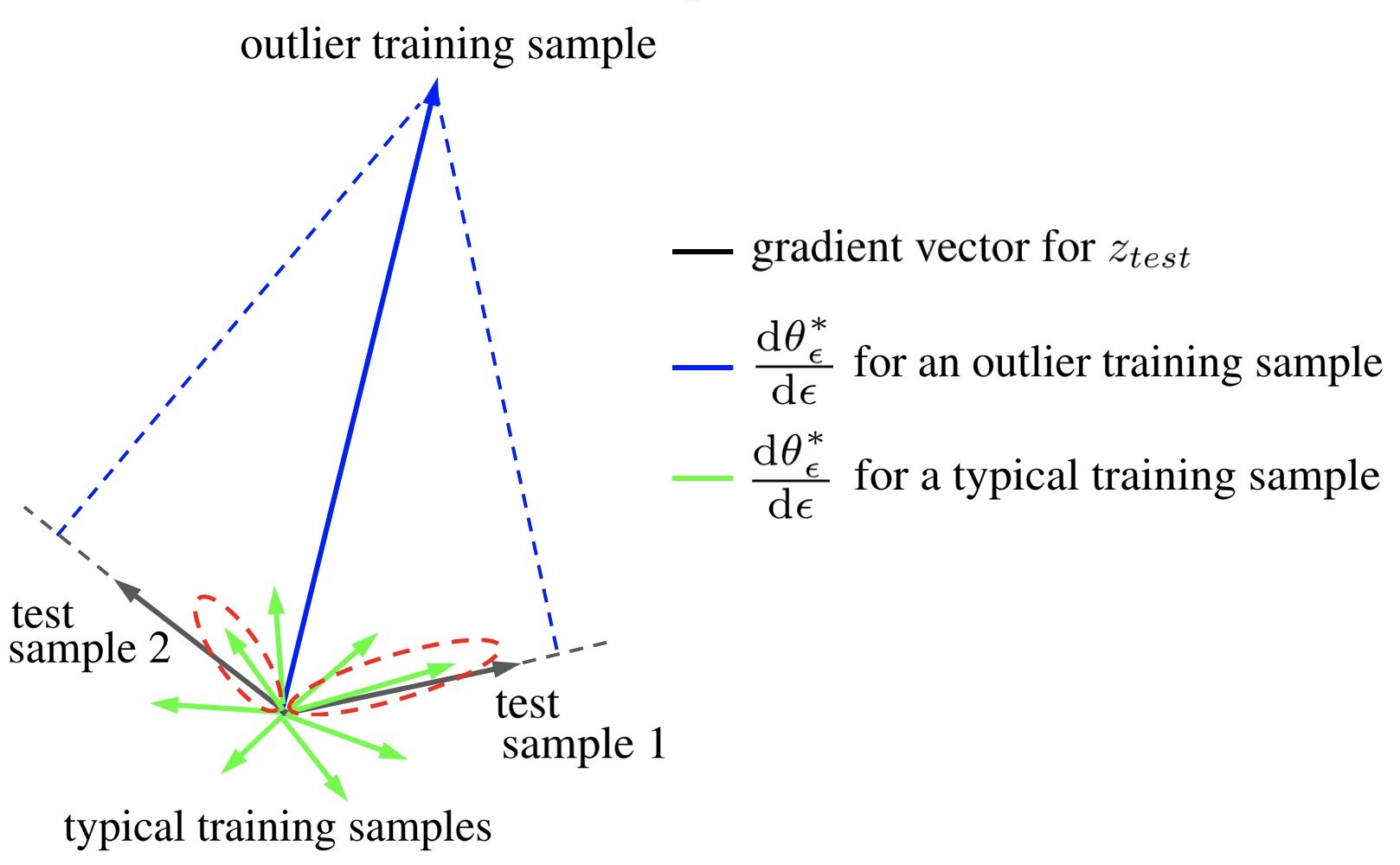
Figure 2: Geometric interpretation of RelatIF. Using IF, the influence of $z_{i}$ on $z_{\text{test}}$ is equal to the projection length of the change in parameters vector onto the test sample’s (negative) loss gradient. Observe how the same outlier training example becomes the top influential example for two different test samples due to the very large magnitude effect on the model parameters. RelatIF, instead uses cosine similarity to identify the top influential examples, and thus return those in the red dotted circles.

The equivalence between $\theta$-RelatIF and the cosine similarity between a test point gradient $g_{\text{test}}$ and a change in the parameters vector $\frac{\mathrm{d}\theta^{*}_{i,\epsilon_{i}}}{\mathrm{d}\epsilon_{i}}$ is straighforward. The norm of the test sample gradient $\lVert g_{\text{test}}\rVert$ is independent of $i$, and so it follows that

$$\operatorname*{arg\,max}_{i} \frac{\mathcal{I}_{\text{test},i}}{\lVert H_{\theta^{*}}^{-1}g_{i}\rVert}=\operatorname*{arg\,max}_{i}\frac{{\langle-g_{\text{test}},-H_{\theta^{*}}^{-1}g_{i}\rangle}}{\lVert g_{\text{test}}\rVert\lVert H_{\theta^{*}}^{-1}g_{i}\rVert}.$$

Further, $\ell$-RelatIF can also be interpreted as cosine similarity, but not using the standard euclidean inner product. Instead, it is cosine similarity under the inner product $\langle a,b\rangle=a^{T}F^{-1}_{\theta^{*}}b$.

Computational considerations

Computing influence can be challenging, especially in larger models. The terms in the denominator introduced by RelatIF pose a further computational challenge. We outline our approach to computing relative influence in larger models in Appendix C. It builds off the inverse Hessian vector product approximations used by Koh & Liang (2017), but makes some further approximations, principally motivated by K-FAC (Martens & Grosse, 2015)

4 Experimental Results

	Logistic Regression on MNIST				ConvNet on CIFAR10
	Infl. Set Cardinality		Infl. Set Probability		Infl. Set Cardinality		Infl. Set Probability
Method	top 1	top 5	top 1	top 5	top 1	top 5	top 1	top 5
IF	2704	4984	$0.168\pm 0.16$	$0.268\pm 0.21$	2279	4869	$0.431\pm 0.21$	$0.511\pm 0.21$
$\theta$-RelatIF	8582	29317	$0.929\pm 0.16$	$0.922\pm 0.17$	8264	26381	$0.918\pm 0.15$	$0.910\pm 0.16$
$\ell$-RelatIF	8776	30431	$0.938\pm 0.16$	$0.930\pm 0.17$	8336	26550	$0.931\pm 0.14$	$0.920\pm 0.15$

Table 1: Comparing the set of top influential training examples recovered using IF and RelatIF for a logistic regression trained on MNIST and a ConvNet trained on CIFAR10 data sets. The number of test samples for each data set is $10000$. For each test sample, the top (1 or 5) positively influential training example is recovered and added to the influential set (duplicates are removed). The cardinality of this set as well of the mean probability ($\pm$std-dev) of its elements are reported for IF and different variations of RelatIF. The larger cardinality of the set is an indication of recovering more specific (as opposed to globally) influential examples. Higher likelihood for the elements of the set shows more typical examples (and fewer outliers) are retrieved.

We empirically assess the use of relative influence (RelatIF) as a technique for explaining model predictions. We compare the examples identified by RelatIF to the baseline examples identified using influence functions (IF) or k-nearest neighbors (k-NN). We consider three models and data sets: logistic regression trained on MNIST handwritten digit data set (LeCun et al., 1998), a convolutional neural network (ConvNet) trained on CIFAR10 object recognition data set (Krizhevsky et al., 2009), and a long short-term memory (LSTM) network trained for classifying names based on their language of origin.

4.1 Quantitative Analysis

It is known that the training examples selected via IF are often high-loss, i.e., they are either mislabelled, outliers, or a-typical (Hampel, 1974; Campbell, 1978; Cook & Weisberg, 1982; Croux & Haesbroeck, 2000). We further demonstrate that the sets of top-k examples maximizing $\mathcal{I}_{\text{test},i}$ for different test inputs often have a big overlap. We quantify these properties and contrast them to the examples selected via RelatIF.

Overlap and probability

We train a logistic regression model on MNIST, as well as a ConvNet on CIFAR10. In each setup we identify the top-k positively influential examples for 10,000 test inputs using both IF and RelatIF. For each of the selected examples, we examine the class probabilities returned by the model. Since these models are trained based on a negative-log-likelihood loss function, output probabilities are indicative of the loss. We also examine the extent to which these examples overlap by considering the cardinality of the set of top-k examples across all 10,000 test inputs. The maximum feasible cardinality is $k\times 10,000$ (limited by the number of training examples), which is achieved when unique training examples are identified as explanatory for each of the test samples. A cardinality smaller than this maximum implies that there is an overlap between the influential examples. The results are tabulated in Table 1.

We find that in all of our experiments, the positively influential points identified by RelatIF have little overlap. They also have much higher probability under the model’s conditional distribution, and hence have lower loss. For example, in our ConvNet/CIFAR10 setup, the top-5 highest influential training examples identified by IF across all 10,000 test inputs is a set of only 4,869 examples with mean probability 0.511. In contrast, when identified with RelatIF, the set contains on average 26,430 examples with mean probability 0.928.

Method	$\Delta\ell_{\text{test}}$	$\lVert\Delta\theta\rVert$	$\sqrt{\sum(\Delta\ell_{i})^{2}}$
IF	$0.0106\pm 0.0023$	$0.039\pm 0.003$	$0.879\pm 0.092$
$\theta$-RelatIF	$0.0084\pm 0.0027$	$0.004\pm 0.001$	$0.080\pm 0.033$
$\ell$-RelatIF	$0.0086\pm 0.0028$	$0.004\pm 0.002$	$0.068\pm 0.036$
Nearest-N	$0.0048\pm 0.0025$	$0.003\pm 0.001$	$0.044\pm 0.024$

Table 2: The change in loss at a test sample ($\Delta\ell_{\text{test}}$), compared with the norm of the change in parameters ($\lVert\Delta\theta\rVert$) and root sum of square change in loss over the training set ($\sqrt{\sum(\Delta\ell_{i})^{2}}$). The results come from removing the mostly positively influential training sample as determined by different methods, then retraining the model (i.e., leave-one-out retraining). The model is a logistic regression trained on MNIST. The experiment is repeated for 100 randomly selected test samples. The mean $\pm$ standard error are reported. While IF identifies the training samples having the largest influence on the test sample’s loss, RelatIF finds comparably influential samples with an order of magnitude smaller global effects. A nearest neighbor baseline is included for comparison.

Global effects

We are also interested in quantifying the global effect of the top influential examples selected by each method. We train a logistic regression model on MNIST to convergence, explicitly seeding all sources of randomness. We then pick 100 test samples uniformly at random. For each of these test samples, we identify the most positively influential training example using IF and RelatIF. We then retrain the model without that training example, maintaining the same random seed, and measure the effects. Specifically, we consider how the removal of that training example affects the root squared error across the training set, as well as how it affects the learned model parameters. The results are tabulated in Table 2.

We find that the examples identified by IF have a much stronger global impact on the model than do those identified by RelatIF. Using IF, the removal of the top influential examples results in a mean change in parameters of 0.039 and a root mean squared change in loss of 0.879. Using RelatIF, these changes are an order of magnitude smaller.

4.2 Qualitative Analysis

The purpose of our qualitative experiments is to evaluate RelatIF in the context of example-based explanations of model predictions. RelatIF is derived by explicitly minimizing the global effect on the model. As a result, the examples selected by RelatIF are specific to the given test sample, and the effect of examples with large global influence is diminished.

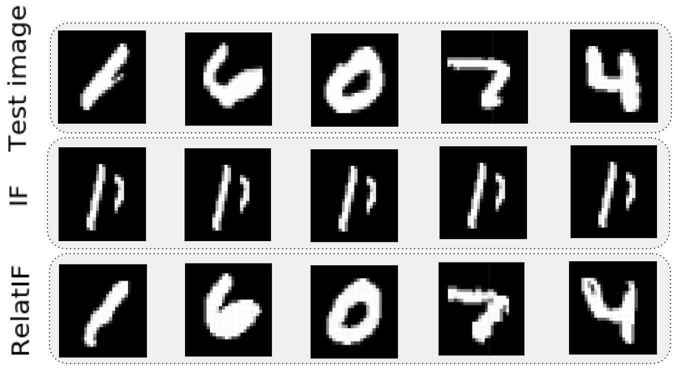
Figure 3: The most positively influential training examples suggest by IF and RelatIF. Test samples are in the first row. IF selects the same (high-loss) training example as the top influential example for all the test images. In contrast, RelatIF discovers training examples that are specific to each of the test images.

We find that examples identified by IF have significantly more global influence. An illustration of this effect for a logistic regression trained on MNIST is presented in Fig. 3. As this figure shows, based on IF, a single high-loss training example is the most positively influential example for a number of different test images. We argue that explaining the model prediction for all of these different test samples using a single high-loss (e.g., outlier) training example is not intuitive and may undermine the user’s trust. RelatIF addresses this issue and enables us to identify examples that are more relevant to each specific test input.

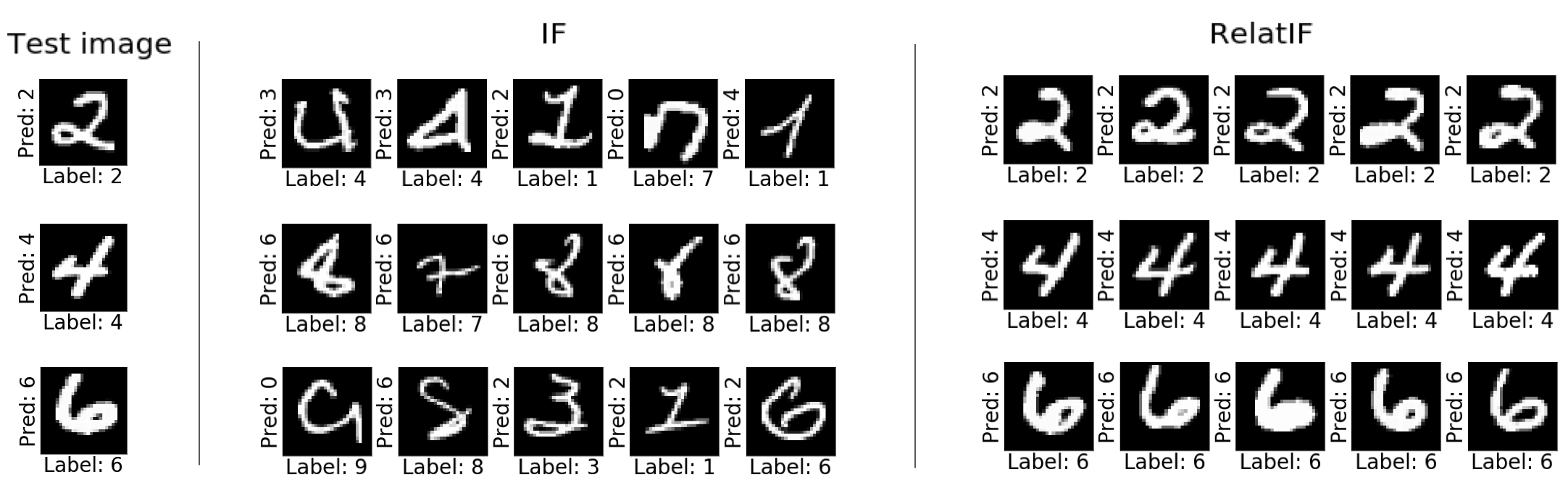
Figure 4: Comparison of the top positively influential training examples recovered by IF and RelatIF for logistic regression on MNIST. Each row shows a test sample and the top five positively influential training examples for the predicted label selected by each method. The true class and the predicted label for each example are provided. Observe how most of the examples selected by IF are unusual and misclassified, despite the training set containing examples with higher visual similarity (as suggested by RelatIF).

We study the effectiveness of RelatIF for generating example-based explanations under different types of models and data sets. Fig. 4 shows the explanations produced for a logistic regression trained on MNIST. For each test image, the top five positively influential training examples for the predicted label identified by IF and RelatIF are presented. Most of the examples selected by IF are misclassified training examples (due to their large global influence on the model parameters). In contrast, RelatIF identifies visually similar examples. We understand this to be the result of constraining global influence, thereby putting more importance on the similarity of the test/train gradients.

Now we make the model a bit more complex and try to explain a ConvNet trained on CIFAR10 data set. Fig. 5 shows the generated explanation for a correctly classified (dog) and a misclassified (truck) test sample. Interestingly, we can see that a set of visually similar dog training images are specifically helpful for predicting the label dog for the given test image. In the case of the red truck, the explanation by RelatIF suggests that the presence of a number of red cars (with similar shade of color and shape) specifically influences the model to classify it as a car. For more examples of CIFAR10 explanations see Appendix H.

A similar experiment is conducted for a character-level LSTM network trained for classifying names based on their language of origin. The data set consists of $20,000$ surnames from $18$ different languages. Due to the large number of model parameters, similar to Koh & Liang (2017), in this experiment we used only the last layer parameters for computing influence scores. Table 3 shows the generated explanation for classifying surname “Vasyukov” as Russian. The examples identified by IF are all Russian names that are misclassified as Japanese. In contrast, all of the examples identified by RelatIF are Russian names that end with “kov”, similar to the test input.

The explanations provided for these models enable the end user to assess the reliability of the generated prediction. The user can confirm, reject or modify the model decision by inspecting the extracted evidence from the training set. This is especially useful when the model is not confident in its prediction. For an example of this application see Appendix E.

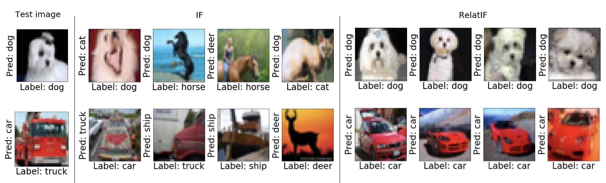
Figure 5: Generating example-based explanations using IF and RelatIF for the predicted label by a ConvNet trained on CIFAR10. Each row shows a test sample and the top five positively influential training examples for the predicted label selected by each method. The true class and the predicted label for each example is marked. Compared to IF, RelatIF is able to retrieve training examples with higher visual similarity to the test image.

	IF	RelatIF
Test Input: Vasyukov (Russian)	Tokovoi (Japanese)	Gasyukov (Russian)
	Nasikan (Japanese)	Tsayukov (Russian)
	Bakai (Japanese)	Tzarakov (Russian)
	Mihailutsa (Japanese)	Tzayukov (Russian)
	Jugai (Japanese)	Haryukov (Russian)
	Mikhailutsa (Japanese)	Tsarakov (Russian)

Table 3: Generating Explanation for text classification. The model is a character-level RNN trained for classifying names based on their language of origin. The most positively influential training examples selected based on IF and RelatIF are listed. The language in parentheses shows the predicted label. The true label for all examples shown is Russian. Observe how the examples identified by IF are all misclassified as Japanese, while the examples identified by RelatIF end with “kov”, which is similar to the test input.

4.3 Comparison to Nearest-Neighbors

Here we compare a test sample’s k-nearest neighbors (k-NNs) to the samples returned using RelatIF. For a quantitative comparison we use the same MNIST and CIFAR10 experimental setups discussed in Section 4.1. We consider the overlap between the top-k samples identified by RelatIF, and the k-NNs ($l_{2}$ distance) for k in $\{1,5,10,20\}$. In the logistic regression model on MNIST we find the overlap ranges from 26-35%, increasing with k. A substantial overlap, but still indicative of a fundamentally different set of points. In the CNN on CIFAR10 we find much less overlap, only 2.6-5.6%, decreasing with k. By comparison, the overlap between the top-k samples identified by IF and the k-NNs is 1.3-2.7% in the logistic regression model, and 0.67-1.24% in the CNN. This indicates that the points returned by RelatIF are closer in $l_{2}$ distance to the test sample than those returned by IF.

A qualitative comparison finds a significant difference between the k-NNs and the samples returned by RelatIF (see Appendix G). These examples are abundant and easily found for our CNN on CIFAR10. We have included some of these examples in the appendix.

5 Related work

Influence functions (IF) were originally proposed by Hampel (1974). Methods based on IF are identical to the infinitesimal jackknife, which was introduced earlier in an independent work on robust statistics by Jaeckel (1972). The connection between IF and infinitesimal jackknife was recognized by (Efron, 1982).

Koh & Liang (2017) use IF to identify influential training examples in a modern machine learning context. They further demonstrate that influence functions can be used to identify mislabelled data and generate adversarial training examples(Koh et al., 2018). More recently, Koh et al. (2019) use IF to approximate the effects of re-weighting groups of training examples.

A range of approaches have been introduced to identify training examples for interpreting predictions. One such approach was recently proposed by Khanna et al. (2019). The authors use Fisher kernels to identify points that are “most responsible” for a given set of predictions. They demonstrate that in the case of a negative log-likelihood loss function and with a specific choice of hyper-parameters, their approach coincides with IF. Another recent contribution is due to Ghorbani & Zou (2019). The authors propose a new form of data valuation which identifies important examples or subsets of the data using Shapley values.

Other approaches to example-based explanation include the extraction of prototypical data, as well as generating counter-factual examples. Bien & Tibshirani (2011) propose a method to select prototypes for interpretable classification. Kim et al. (2016) introduce a method for explaining the data set by identifying its prototypes and ”criticisms” and argue that a-typical data must also be extracted. Chang et al. (2019) introduce a novel method for generating counter-factual images to be used as an explanation.

Finally, the effect of example-based explanations on user trust have been studied in the human-computer interaction community. One of the most recent study is presented in (Zhou et al., 2019). For each test sample, Zhou et al. select examples maximizing influence. They provide these selected training examples along with model prediction and study the effect on the users’ trust in the predictive model. A similar set of experiments can be found in (Cai et al., 2019). In this study, the effect on users’ trust is compared for different types of “explanatory” examples.

6 Discussion

In this work we introduce relative influence (RelatIF) and show that it identifies more intuitive examples than those identified by influence functions (IF). In particular, we demonstrate that, unlike examples identified by IF, which tend to be atypical or misclassified, and otherwise unrelated to the test sample, examples identified by RelatIF seem to be more specific to test sample. As a result, we believe that RelatIF may be superior at identifying explanatory examples that a user may find intuitive and acceptable. The desiderata of example-based explanations are case specific, and therefore one cannot make an absolute comparison of IF versus RelatIF. A data scientist fitting a model to a data set containing spurious samples may very well wish to see the examples identified by both IF and RelatIF. We believe a large user study, which is beyond the scope of this paper, may shed light on the relative strengths and weaknesses of RelatIF, and lead to further insight.

Acknowledgements

We thank the reviewers for their feedback and suggestions. We are grateful to all the input we received from our colleagues and advisors at Element AI.

A Connection between the Fisher and Hessian

The Fisher information matrix of a conditional distribution parameterized by $\theta$, $p_{\theta}(y|x_{i})$, where we do not have an explicit representation for $p(x)$, is

$$F_{\theta} =\frac{1}{n}\sum_{i=1}^{n}\mathbb{E}_{p_{\theta}}\nabla_{\theta}\log p_{\theta}(y|x_{i})\nabla_{\theta}\log p_{\theta}(y|x_{i})^{T}$$

$$=\frac{1}{n}\sum_{i=1}^{n}\Big{[}\underbrace{\mathbb{E}_{p_{\theta}}\frac{\nabla_{\theta}^{2}p_{\theta}(y|x_{i})}{p_{\theta}(y|x_{i})}}_{=0}-\mathbb{E}_{p_{\theta}}\nabla_{\theta}^{2}\log p_{\theta}(y|x_{i})\Big{]}$$

$$=-\frac{1}{n}\sum_{i=1}^{n}\mathbb{E}_{p_{\theta}}\nabla_{\theta}^{2}\log p_{\theta}(y|x_{i}).$$

The second equality can be obtained by carrying out the differentiation $\nabla_{\theta}^{2}\log p_{\theta}(y|x)$. The third equality critically relies on the expectation being taken with respect to the model’s distribution, as well as being able to switch the order of the expectation and differentiation.

When our model has learned a distribution $p_{\theta}(y|x)$ close to the ”true” distribution $p(y|x)$, we may approximate $F_{\theta}$ by replacing $\mathbb{E}_{p_{\theta}}$ with a Monte Carlo estimate based on the target values, $y_{i}$, in the training set. This gives us

$$F_{\theta}\approx-\frac{1}{n}\sum_{i=1}^{n}\nabla_{\theta}^{2}\log p_{\theta}(y_{i}|x_{i})=H_{\theta}.$$

The final equality with $H_{\theta}$ (as defined in Eq. 2) holds when $\ell(z,\theta)=-\log p_{\theta}(y_{i}|x_{i})$. Therefore, our two expressions for influence, Eq. 3 and Eq. 6, approximately agree when the loss is the negative log likelihood, and $y$ given $x$ is actually distributed as $p_{\theta^{*}}(y|x)$. In practice, we have found that the Fisher and Hessian return similar examples when used to compute $\mathcal{I}_{\text{test},i}$.

B Proofs of RelatIF

Recall Proposition 3.1: Assume that Eq. 4 and Section 2.1 hold with equality. Then Section 3.1 is equivalent to

$$\operatorname*{arg\,max}_{i\in\{1,\ldots,n\}}\frac{\lvert\mathcal{I}_{\text{test},i}\rvert}{\lVert H_{\theta^{*}}^{-1}g_{i}\rVert}.$$ (14)

Proof.

The $\operatorname*{arg\,max}$ in Section 3.1 is just a search over the $n$ examples in our training set. Therefore the solution to Section 3.1 amounts to solving $\operatorname*{\mathrm{max}\vphantom{\mathrm{infsup}}}\lvert\ell(z_{\text{test}},\theta^{*}_{i,\epsilon_{i}})-\ell(z_{\text{test}},\theta^{*})\rvert$ subject to the constraints for each $i$, then choosing the $z_{i}$ for which this quantity is largest. We assume Section 2.1 holds with equality, and so it follows

$$\lvert\ell(z_{\text{test}},\theta^{*}_{i,\epsilon_{i}})-\ell(z_{\text{test}},\theta^{*})\rvert=\lvert\mathcal{I}_{\text{test},i}\epsilon_{i}\rvert.$$

Note, that $\mathcal{I}_{\text{test},i}\epsilon_{i}$ is a linear function in $\epsilon_{i}$. The maximum of its absolute value will therefore be on one of the endpoints imposed by the constraint on $\epsilon_{i}$.

We assume that approximation in Eq. 4 is exact, yielding $\theta^{*}_{i,\epsilon_{i}}-\theta^{*}=-H_{\theta^{*}}^{-1}g_{i}\epsilon_{i}$. Using this equality to describe the change in parameters, the constraint in Section 3.1 can be written as

$$\lVert H_{\theta^{*}}^{-1}g_{i}\epsilon_{i}\rVert^{2}\leq\delta^{2}\implies\lvert\epsilon_{i}\rvert\leq\frac{\lvert\delta\rvert}{\lVert H_{\theta^{*}}^{-1}g_{i}\rVert}.$$

We now have an explicit constraint on $\epsilon_{i}$. Plugging either endpoint of this interval into $\lvert\mathcal{I}_{\text{test},i}\epsilon_{i}\rvert$ yields the same value. Substituting that value into the outer $\operatorname*{arg\,max}$ we get,

$$\operatorname*{arg\,max}_{i\in\{1,\ldots,n\}}\frac{\lvert\mathcal{I}_{\text{test},i}\rvert\lvert\delta\rvert}{\lVert H_{\theta^{*}}^{-1}g_{i}\rVert}.$$

Since $\delta$ does not depend on $i$, it can be dropped from the $\operatorname*{arg\,max}$, and the result follows. ∎

Recall Proposition 3.3: Assume Eq. 8 and Eq. 9 hold with equality. Then Section 3.2 is equivalent to

$$\operatorname*{arg\,max}_{i\in\{1,\ldots,n\}}\frac{\lvert\mathcal{I}_{\text{test},i}\rvert}{\sqrt{\mathcal{I}_{i,i}}}.$$ (15)

Proof.

The proof follows the proof of Proposition 3.1. We need only consider the new constraint. Assuming Eq. 9 holds with equality, we have

$$\ell(z_{j},\theta^{*}_{i,\epsilon_{i}})-\ell(z_{j},\theta^{*})=\mathcal{I}_{j,i}\epsilon_{i}=-g_{j}^{T}F^{-1}_{\theta^{*}}g_{i}\epsilon_{i}.$$

We introduce the notation $g({z})=\nabla_{\theta}\ell(z,\theta^{*})$ to signify the gradient of the loss of a point $z=(x,y)$ sampled from the model’s distribution, $p_{\theta}^{*}$. We substitute into the constraint, which yields

$$\mathbb{E}_{p_{\theta^{*}}}(-g({z})^{T}F^{-1}_{\theta^{*}}g_{i}\epsilon_{i})^{2}\leq\delta^{2}.$$

Expanding and rearranging the left hand side, yields

$$\mathbb{E}_{p_{\theta^{*}}}(g({z})^{T} F^{-1}_{\theta^{*}}g_{i}\epsilon_{i})^{T}(g({z})^{T}F^{-1}_{\theta^{*}}g_{i}\epsilon_{i})$$

$$=g_{i}^{T}F^{-1}_{\theta^{*}}\mathbb{E}_{p_{\theta^{*}}}\big{[}g({z})g({z})^{T}\big{]}F^{-1}_{\theta^{*}}g_{i}\epsilon_{i}^{2},$$

where we have moved the constant terms outside of the expectation. Because our loss functions here is negative log-likelihood, $\mathbb{E}_{p_{\theta^{*}}}[g({z})g({z})^{T}]$ is the is the definition of the Fisher information matrix, $F_{\theta}^{*}$. It agrees with the presentation in Section 2.2 when we replace the expectation over $z=(x,y)$ with $\sum_{j}E_{p_{\theta^{*}}(y|x_{j})}$. Thus the constraint can be reduced to

$$g_{i}^{T}F^{-1}_{\theta^{*}}g_{i}\epsilon_{i}^{2}=\mathcal{I}_{i,i}\epsilon_{i}^{2}\leq\delta^{2}.$$

The Fisher, $F_{\theta^{*}}$, is positive definite, therefore $\mathcal{I}_{i,i}$ is positive, and the constraint is equivalent to $\lvert\epsilon_{i}\rvert\leq\frac{\lvert\delta\rvert}{\sqrt{\mathcal{I}_{i,i}}}$. The rest of the proof follows Proposition 3.1. ∎

C Computational Considerations

Inverting the Hessian

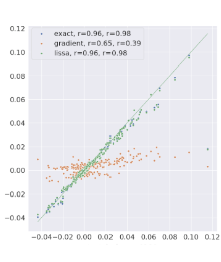
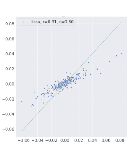
(a) Logistic Regression on MNIST	(b) ConvNet on MNIST	(c) AlexeNet on small ImageNet

Figure 6: Evaluating the accuracy of the estimated error for leave-one-out retraining by influence functions with different hessian approximations. in the figure, “exact” refers to exact Hessian, “gradient” referes to using identity matrix for Hessian and “lissa” refers to using the LiSSA method for approximating inverse Hessian vector products. In the case of AlexNet, the results are only reported for LiSSA due computational/memory complexity. For all of these models a small damping coefficient has been added to the diagonal of the Hessian to make it invertible. As this figure shows, in the case of LiSSA and exact Hessian, the correlation between influence function estimation for change of loss and the actual leave-one-out retraining loss is high.

The Hessian of the total loss, $H_{\theta^{*}}$, is positive definite if $\theta^{*}$ is the local minimum of the objective function. If the requirements for positive definiteness of $H_{\theta}$ are not met, for example because the optimization procedure has not fully converged, we can add a damping term to the Hessian to make it invertible (i.e., $\tilde{H}_{\theta}={H}_{\theta}+\lambda I$ where $I$ is the identity matrix). Adding the damping term is equivalent to $L_{2}$ regularization, and allows us to form a convex quadratic approximation to the loss function.  Koh & Liang (2017) demonstrate that influence functions computed with a damping term still give meaningful results in practice. Empirically we have also found this to be the case (see Fig. 6).

IF and RelatIF in large models

The Hessian of the total loss, $H_{\theta^{*}}$, is a $P$ by $P$ matrix, where $P$ is the number of model parameters. In even just mid-sized models, it becomes near impossible to explicitly form $H_{\theta^{*}}$ in memory. Koh & Liang (2017) propose using LiSSA (Agarwal et al., 2017) to estimate the inverse Hessian vector products needed to compute influence. We have found that this works well in practice after some tuning. However, because the denominator in RelatIF is a function of the training example $z_{i}$ we cannot use the same $s_{\text{test}}$ trick suggested by Koh & Liang (2017). This has led us to explore using a number of block diagonal approximations to the Hessian, principally motivated by K-FAC (Martens & Grosse, 2015). Specifically, we use these approximations to pre-compute the denominator in RelatIF ($\sqrt{\mathcal{I}_{i,i}}$ or $\lVert H^{-1}_{\theta^{*}}g_{i}\rVert$) for every training example $z_{i}$. We are then able to use $s_{\text{test}}$.

D Comparison to support vectors

Consider a soft-SVM optimization problem, with a dimensionality of the feature space lower than the number of training points. Via working with a dual formulation of the objective, one can uncover that the optimal weights $w^{\star}$ lie in the linear span of some training samples, called support vectors (see, e.g., (Shalev-Shwartz & Ben-David, 2014), Ch.15).

Let $\psi(\cdot)$ map inputs $x$ to a feature space. Define a kernel function $K(x_{i},x_{j})={\langle\psi(x_{i}),\psi(x_{j})\rangle}$ for all inputs $x_{i},x_{j}$. Let $w^{*}$ be an output of a solution to a soft-margin SVM.

The support vectors are the training samples indexed by $i$, such that $y_{i}{\langle w^{*},\psi(x_{i})\rangle}\leq 1$, i.e., support vectors are the training samples that are inside the margin or misclassified. By computing the gradients of a soft-SVM objective, one can see that IF induces a ranking of training samples according to $y_{i}y_{test}K(x_{i},x_{test})$, where $\{x_{i}\}_{i}$ are support vectors (IF equals to zero for training samples that are not support vectors). In other words, the highest influence samples are support vectors that are most similar to the test point in the feature space. Similarly, repeating the same calculation for the loss-relative influence, one would rank the support vectors based on $y_{i}y_{test}K(x_{i},x_{test})/\sqrt{K(x_{i},x_{i})}$.

In summary, IF gives a way to distinguish which of the training samples among all support vectors are the ones that are most similar to the test sample in the feature space. RelatIF normalizes this similarity in the feature space by the norm of the training sample in the feature space, which is equivalent to IF evaluated on training samples that are unit vectors in the feature space.

E Application of example-based explanations

Consider the example shown in Fig. 7. The input image in the top left corner is classified as a bird, however, the predicted probability for class plane is also very high. Using RelatIF we can identify the top relevant training examples to each label (i.e., bird and plane) and assess the model’s decision based on them. Comparing the similarity between the test image and relevant training examples to each class, suggests that this image should be classified as a plane. Also, these explanations could be used as a guide to collect more training examples for improving the model performance (e.g., what kind of training examples are useful for correcting a specific misclassification).

F Qualitative comparison of $\theta$-RelatIF and $\ell$-RelatIF

Fig. 8 offers a comparison between the top positively influential training examples recovered by $\ell$-RelatIF and $\theta$-RelatIF. As this figure shows, the examples returned by both method are visually similar.

G Qualitative comparison with k-nearest neighbors

Fig. 9 offers a qualitative comparison between using RelatIF and k-nearest neighbors for explaining the prediction of a ConvNet trained on CIFAR10 data set.

H More explanation examples

Fig. 10 and Fig. 11 offer more examples of using RelatIF and IF for explaining the prediction of a ConvNet trained on CIFAR10 data set.

I The connection between RelatIF and leave-one-out retraining

RelatIF is an approximation for the ratio of change in the test sample loss to global changes of the model (i.e., norm of change in the model parameters or root sum of square change in loss over the training set) resulted from leave-one-out retraining. Table 4 reports this ratio for different methods.

Method	$\Delta\ell_{\text{test}}/{\lVert\Delta\theta\rVert}$	$\Delta\ell_{\text{test}}/\sqrt{\sum(\Delta\ell_{i})^{2}}$
IF	$0.311\pm 0.167$	$0.016\pm 0.008$
$\theta$-RelatIF	$0.459\pm 0.226$	$0.026\pm 0.010$
$\ell$-RelatIF	$0.475\pm 0.229$	$0.027\pm 0.010$
Nearest-N	$0.304\pm 0.182$	$0.018\pm 0.009$

Table 4: The ratio of change in the test loss ($\Delta\ell_{\text{test}}$) to the global changes, i.e., the norm of the change in the model parameters ($\lVert\Delta\theta\rVert$), or root sum of square change in loss over the training set ($\sqrt{\sum(\Delta\ell_{i})^{2}}$). The results come from removing the mostly positively influential training sample as determined by different methods, then retraining the model (i.e., leave-one-out retraining). The model is a logistic regression trained on MNIST. The experiment is repeated for 100 randomly selected test samples. The mean $\pm$ standard error are reported. One can approximate the leave-one-out change of these ratios using $\theta$-RelatIF and $\ell$-RelatIF, respectively. Note that these ratios are higher for the samples identified by RelatIF than for those identified by IF or NN. This is due to the fact that RelatIF identifies the points that maximize these ratios.

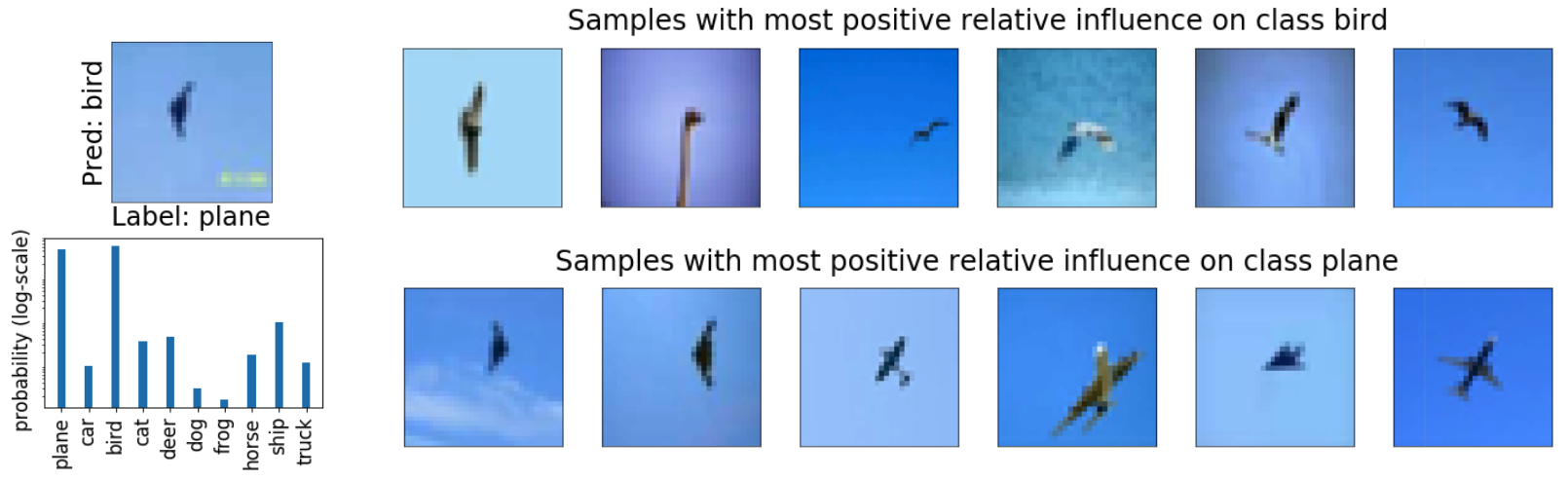
Figure 7: Using RelatIF to identify training examples with the top positive relevant influence on the the predicted (bird) and true label (plane).

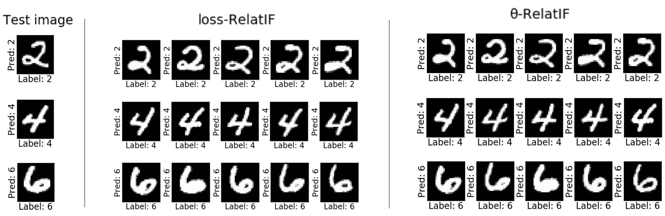
Figure 8: Comparison of the top positively influential training examples recovered by $\ell$-RelatIF and $\theta$-RelatIF. The classifier is a logistic regression trained on MNIST. Each row shows a test sample and the top five positively influential training examples for the predicted label selected by each method. The true class and the predicted label for each example is marked. The example returned by both method are visually similar.

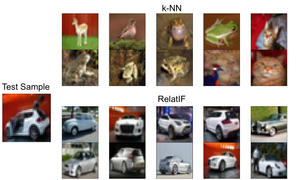
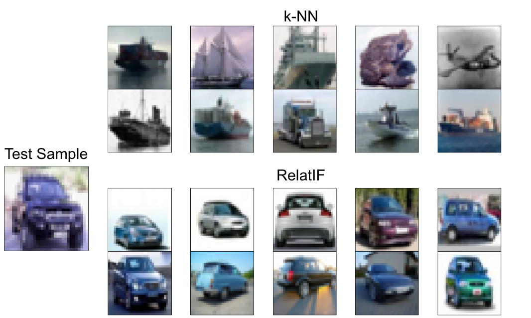
Figure 9: Comparing the k-nearest neighbors (k-NN) to the most (positive) relatively influential samples (RelatIF) for a convolutional neural network trained on CIFAR10. The two test samples were correctly classified by the model. The k-nearest neighbors are similar in pixel composition, but are semantically different from the test sample. They provide no evidence to explain why the model has correctly classified the test sample. Conversely, the samples returned by RelatIF are of the matching class. They suggest the model has been exposed to relevant training data, and has learned something useful.

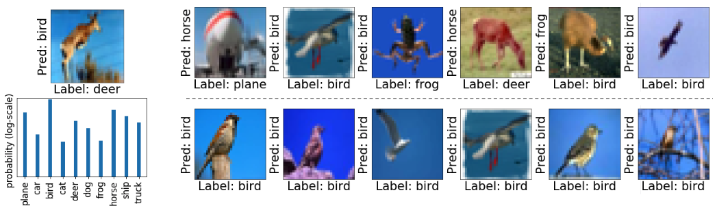
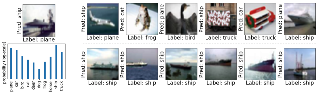
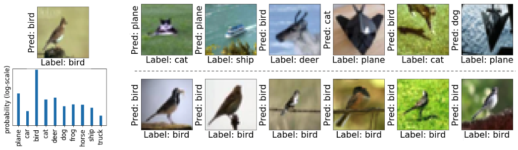
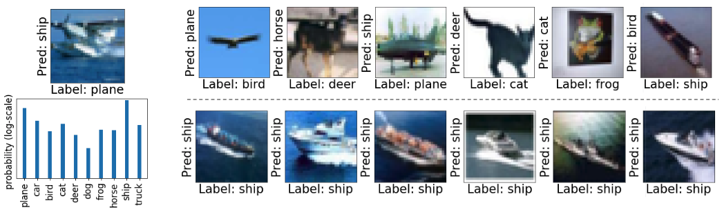
Figure 10: Generating example-based explanation using IF and RelatIF for the model prediction. The model is a ConvNet trained on CIFAR10 data set. For each test sample in the left column, the recovered training examples for explaining the model prediction using IF and RelatIF are depicted in the first and second row, respectively.

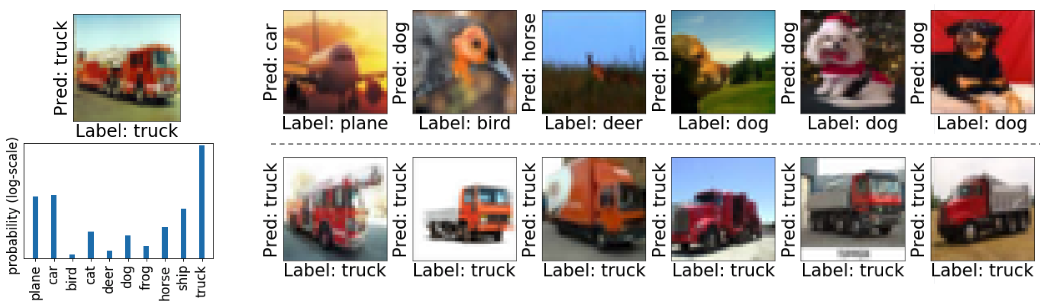
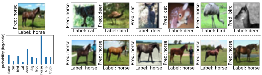
Figure 11: Generating example-based explanation using IF and RelatIF for the model prediction. The model is a ConvNet trained on CIFAR10 data set. For each test sample in the left column, the recovered training examples for explaining the model prediction using IF and RelatIF are depicted in the first and second row, respectively.

References

- Agarwal et al. (2017) Naman Agarwal, Brian Bullins, and Elad Hazan. Second-order stochastic optimization for machine learning in linear time. The Journal of Machine Learning Research, 18(1):4148–4187, 2017.
- Bien & Tibshirani (2011) Jacob Bien and Robert Tibshirani. Prototype selection for interpretable classification. Ann. Appl. Stat., 5(4):2403–2424, 12 2011. doi: 10.1214/11-AOAS495.
- Cai et al. (2019) Carrie J. Cai, Jonas Jongejan, and Jess Holbrook. The effects of example-based explanations in a machine learning interface. In Proceedings of the 24th International Conference on Intelligent User Interfaces, IUI ’19, 2019.
- Campbell (1978) Norm A Campbell. The influence function as an aid in outlier detection in discriminant analysis. Journal of the Royal Statistical Society: Series C (Applied Statistics), 27(3):251–258, 1978.
- Chang et al. (2019) Chun-Hao Chang, Elliot Creager, Anna Goldenberg, and David Duvenaud. Explaining image classifiers by adaptive dropout and generative in-filling. In International Conference on Learning Representations, 2019.
- Cook & Weisberg (1982) R Dennis Cook and Sanford Weisberg. Residuals and influence in regression. New York: Chapman and Hall, 1982.
- Croux & Haesbroeck (2000) Christophe Croux and Gentiane Haesbroeck. Principal component analysis based on robust estimators of the covariance or correlation matrix: influence functions and efficiencies. Biometrika, 87(3):603–618, 2000.
- Doshi-Velez & Kim (2017) Finale Doshi-Velez and Been Kim. Towards a rigorous science of interpretable machine learning. arXiv preprint arXiv:1702.08608, 2017.
- Efron (1982) Bradley Efron. The jackknife, the bootstrap, and other resampling plans, volume 38. Society for Industrial and Applied Mathematics, 1982.
- Ghorbani & Zou (2019) Amirata Ghorbani and James Y. Zou. Data shapley: Equitable valuation of data for machine learning. In ICML, 2019.
- Goodman & Flaxman (2017) Bryce Goodman and Seth Flaxman. European union regulations on algorithmic decision-making and a “right to explanation”. AI Magazine, 38(3):50–57, 2017.
- Hampel (1974) Frank R Hampel. The influence curve and its role in robust estimation. Journal of the American Statistical Association, 69(346):383–393, 1974.
- Jaeckel (1972) Louis A Jaeckel. The infinitesimal jackknife. Bell Telephone Laboratories, Murray Hill, NJ, 1972.
- Khanna et al. (2019) Rajiv Khanna, Been Kim, Joydeep Ghosh, and Sanmi Koyejo. Interpreting black box predictions using fisher kernels. In Kamalika Chaudhuri and Masashi Sugiyama (eds.), Proceedings of Machine Learning Research, volume 89 of Proceedings of Machine Learning Research, pp. 3382–3390. PMLR, 16–18 Apr 2019.
- Kim et al. (2016) Been Kim, Rajiv Khanna, and Oluwasanmi O Koyejo. Examples are not enough, learn to criticize! criticism for interpretability. In D. D. Lee, M. Sugiyama, U. V. Luxburg, I. Guyon, and R. Garnett (eds.), Advances in Neural Information Processing Systems 29, pp. 2280–2288. Curran Associates, Inc., 2016.
- Kim et al. (2017) Been Kim, Martin Wattenberg, Justin Gilmer, Carrie Cai, James Wexler, Fernanda Viegas, and Rory Sayres. Interpretability beyond feature attribution: Quantitative testing with concept activation vectors (tcav). arXiv preprint arXiv:1711.11279, 2017.
- Koh & Liang (2017) Pang Wei Koh and Percy Liang. Understanding black-box predictions via influence functions. In Proceedings of the 34th International Conference on Machine Learning-Volume 70, pp. 1885–1894. JMLR. org, 2017.
- Koh et al. (2018) Pang Wei Koh, Jacob Steinhardt, and Percy Liang. Stronger data poisoning attacks break data sanitization defenses. arXiv preprint arXiv:1811.00741, 2018.
- Koh et al. (2019) Pang Wei Koh, Kai-Siang Ang, Hubert HK Teo, and Percy Liang. On the accuracy of influence functions for measuring group effects. arXiv preprint arXiv:1905.13289, 2019.
- Krizhevsky et al. (2009) Alex Krizhevsky, Geoffrey Hinton, et al. Learning multiple layers of features from tiny images. Technical report, Master’s thesis, Department of Computer Science, University of Toronto, 2009.
- LeCun et al. (1998) Yann LeCun, Léon Bottou, Yoshua Bengio, Patrick Haffner, et al. Gradient-based learning applied to document recognition. Proceedings of the IEEE, 86(11):2278–2324, 1998.
- Lipton (2016) Zachary C Lipton. The mythos of model interpretability. arXiv preprint arXiv:1606.03490, 2016.
- Lundberg & Lee (2017) Scott M Lundberg and Su-In Lee. A unified approach to interpreting model predictions. In Advances in Neural Information Processing Systems, pp. 4765–4774, 2017.
- Martens (2014) James Martens. New insights and perspectives on the natural gradient method. arXiv preprint arXiv:1412.1193, 2014.
- Martens & Grosse (2015) James Martens and Roger Grosse. Optimizing neural networks with kronecker-factored approximate curvature. In International Conference on Machine Learning, pp. 2408–2417, 2015.
- Ribeiro et al. (2018) Marco Tulio Ribeiro, Sameer Singh, and Carlos Guestrin. Anchors: High-precision model-agnostic explanations. In Thirty-Second AAAI Conference on Artificial Intelligence, 2018.
- Shalev-Shwartz & Ben-David (2014) Shai Shalev-Shwartz and Shai Ben-David. Understanding machine learning: From theory to algorithms. Cambridge university press, 2014.
- Ting & Brochu (2018) Daniel Ting and Eric Brochu. Optimal subsampling with influence functions. In Advances in Neural Information Processing Systems, pp. 3650–3659, 2018.
- Zhou et al. (2019) Jianlong Zhou, Zhidong Li, Huaiwen Hu, Kun Yu, Fang Chen, Zelin Li, and Yang Wang. Effects of influence on user trust in predictive decision making. In Extended Abstracts of the 2019 CHI Conference on Human Factors in Computing Systems, CHI EA ’19, pp. LBW2812:1–LBW2812:6, New York, NY, USA, 2019. ACM. ISBN 978-1-4503-5971-9. doi: 10.1145/3290607.3312962.