Time-dependent optimized coupled-cluster method for multielectron dynamics III: A second-order many-body perturbation approximation

Abstract

We report successful implementation of the time-dependent second-order many-body perturbation theory using optimized orthonormal orbital functions called time-dependent optimized second-order many-body perturbation theory [TD-OMP2] to reach out to relatively larger chemical systems for the study of intense-laser-driven multielectron dynamics. We apply this method to strong-field ionization and high-order harmonic generation (HHG) of Ar. The calculation results are benchmarked against ab initio time-dependent complete-active-space self-consistent field (TD-CASSCF), time-dependent optimized coupled-cluster double (TD-OCCD), and time-dependent Hartree-Fock (TDHF) methods, as well as a single active electron (SAE) model to explore the role of electron correlation.

I Introduction

Laser-driven multielectron dynamics has become an active area of research, thanks to the remarkable advance in laser technologies, which has made it possible to measure and control the electronic motion corkum2007attosecond ; krausz2009attosecond ; itatani2004 ; goulielmakis2010real ; sansone2010electron ; schultze2010 ; klunder2011probing ; belshaw2012observation ; calegari2014 ; smirnova2009high . Atoms and molecules interacting with laser pulses of intensity $\gtrsim 10^{14}\,{\rm W/cm}^{2}$ in the visible to mid-infrared spectral range, exhibit highly, even nonperturbatively nonlinear response such as above-threshold ionization (ATI), tunneling ionization, nonsequential double ionization (NSDI), and high-order harmonic generation (HHG). The HHG process is one of the key elements in the study of light-matter interaction in the attosecond time-scale, delivering ultrashort coherent light pulses in the extreme-ultraviolet (XUV) to the soft x-ray regions, which carry the information on the electronic structure and dynamics of the generating medium. antoine1996attosecond The HHG spectra are characterized by a plateau where the intensity of the emitted radiation remains nearly constant up to many orders, followed by an abrupt cutoff.

In principle, the multielectron dynamics and electron correlation ishikawa2015review ; tikhomirov2017high ; likumar ; PhysRevLett.santra are exactly described by the time-dependent Schrödinger equation (TDSE). However, direct numerical integration of TDSE is not feasible for systems with more than two electrons parker1998intense ; parker2000time ; pindzola1998time ; laulan2003correlation ; ishikawa2005above ; feist2009probing ; ishikawa2012competition ; sukiasyan2012attosecond ; vanroose2006double ; horner2008classical . As a result, single-active-electron (SAE) approximations has been widely used krause1992jl ; kulander1987time , in which only the outermost electron is explicitly treated under the effect of the other electrons modeled by an effective potential. Whereas SAE has been useful in numerically exploring different strong-field phenomena, the electron correlation is missing in this approximation.

Therefore, various tractable ab initio methods have actively been developed for theoretical description of correlated multielectron dynamics in intense laser fields. Among the most reliable approaches to serve the purpose are the multiconfiguration time-dependent Hartree-Fock (MCTDHF) method caillat2005correlated ; kato2004time ; nest2005multiconfiguration ; haxton2011multiconfiguration ; hochstuhl2011two and time-dependent complete-active-space self-consistent-field (TD-CASSCF) method sato2013time ; sato2016time . In MCTDHF, the electronic wavefunction is expressed in terms of full configuration interaction (FCI) expansion, $\Psi(t)=\sum_{\bm{I}}C_{I}(t)\Phi_{\bm{I}}(t)$, where both CI coefficients $\{C_{\bm{I}}(t)\}$ and occupied spin-orbitals $\{\psi_{p}(t)\}$ constituting Slater determinants $\{\Phi_{\bm{I}}(t)\}$ are propagated in time. The TD-CASSCF method flexibly classifies occupied orbital space into frozen-core (doubly occupied and fixed in time), dynamical-core (doubly occupied but propagated in time) and active (fully correlated and propagated in time) subspaces. Though accurate and powerful, the computational cost of the MCTDHF and TD-CASSCF methods scales factorially with the number of correlated electrons.

More approximate and thus less demanding methods such as the time-dependent restricted-active-space self-consistent field (TD-RASSCF),miyagi2013time ; miyagi2014time ; haxton2015two and time-dependent occupation-restricted multiple-active-space (TD-ORMAS) sato2015time have been developed by further flexibly classifying active orbital sub-space to target larger chemical systems by limiting CI expansion of the wavefunction up to a manageable level. The TD-RASSCF and TD-ORMAS methods achieve a polynomial, instead of factorial, cost scaling, and state-of-the-art real-space implementations have turned out to be of great utility. haxton2015two ; sato2016time ; Omiste:2017 ; orimo2018implementation (See Ref. 12 for a review of ab initio wavefunction-based methods for multielectron dynamics, Ref. 41 and references therein for extension to correlated electron-nuclear dynamics, and Ref. 42 for a perspective on multiconfiguration approaches for indistinguishable particles.) Nevertheless, truncated-CI-based methods, even with time-dependent orbitals, have a general drawback of not being size extensive.

To regain the size-extensivity at the same level of truncation, we have recently derived and numerically implemented a time-dependent optimized coupled-cluster (TD-OCC) method sato2018communication using optimized orthonormal orbitals where both orbitals and amplitudes are time-dependent. Our TD-OCC method is the time-dependent formulation of the stationary orbital optimized coupled-cluster method. sherrill1998energies ; krylov1998size We have implemented the TD-OCC method with up to triple excitation amplitudes (TD-OCCD and TD-OCCDT), and applied it to multielectron dynamics in Ar induced by a strong laser pulse to obtain a good agreement with the fully-correlated TD-CASSCF method within the same active orbital space. In earlier work, Kvaal reported kvaal2012ab an orbital adaptive coupled-cluster (OATDCC) method built upon the work of Arponen using biorthogonal orbitals; arponen1983variational though, applications to laser-driven dynamics have not been addressed. The polynomial scaling TD-OCC sato2018communication or the OATDCC kvaal2012ab method can reduce the computational cost to a large extent in comparison to the general factorially scaling MCTDHF methods.

As a cost-effective approximation of the TD-OCCD method, we have recently developed a method called TD-OCEPA0pathak2020timedependent based on the simplest version of the coupled-electron pair approximation,meyer1971ionization ; ahlrichs1985coupled ; wennmohs2008comparative ; neese2009efficient ; kollmar2010coupled ; malrieu2010ability or equivalently the linearized CCD approximation,vcivzek1966correlation popular in quantum chemistry. The computational cost of the TD-OCEPA0 method scales as $N^{6}$, with $N$ being the number of active orbitals. Although this is the same scaling as that of the parent TD-OCCD method, TD-OCEPA0 is much more efficient than TD-OCCD due to the linearity of amplitude equations and avoidance of a separate solution for the de-excitation amplitudes, resulting from the Hermitian structure of the underlying Lagrangian.pathak2020timedependent

To enhance the applicability to even larger chemical systems, we are looking for further approximate versions with a lower computational scaling in the TD-OCC framework. The coupled-cluster method is intricately connected with the many-body perturbation theory. It allows one to obtain finite-order perturbation theory energies and wavefunction from the coupled-cluster equations. bartlettreviewmbptcc The computation of the second-order energy requires the first-order wavefunction, and only doubly excited determinants have contributions in the first-order correction to the reference wavefunction. Thus, second-order many-body perturbation theory (MP2) can be seen as an approximation to the coupled-cluster double (CCD) method, having a lower $N^{5}$ scaling.

The MP2 method with optimized orbitals has been developed by Bozkaya et al. bozkaya2011quadratically for the stationary electronic structure calculations by minimization of the so-called MP2-$\Lambda$ functional. In earlier work, the optimization of the MP2 energy was based on the minimization of the Hylleraas functional with respect to the orbital rotation. adamowicz1987optimized ; neese2009assessment While both of these techniques provide identical energy at the stationary point, the $\Lambda$ functional-based derivation has an advantage that it can be easily extended to higher-order many-body perturbation theory.bozkaya2011orbital

In this article, we propose time-dependent orbital optimized second-order many-body perturbation theory (TD-OMP2) as an approximation to the TD-OCCD method, based on the time-dependent (quasi) variational principle. The TD-OMP2 method inherits important features of size extensivity and gauge invariance from TD-OCC, with a reduced computational cost of $O(N^{5})$. As a first test case, we apply the TD-OMP2 method to electron dynamics in Ar atom irradiated by a strong laser field, and compare the results with those computed at SAE, TDHF, TD-OCCD, and TD-CASSCF levels to understand where really TD-OMP2 stands in describing the effects of correlation in the laser-driven multielectron dynamics. It should be emphasized that the present TD-OMP2 method, albeit named after a perturbation theory, can be applied to laser-induced, nonperturbative electron dynamics, since the laser-electron interaction is fully (nonperturbatively) included in the zeroth-order description with time-dependent orbitals.

This paper is organized as follows. Our formulation of the TD-OMP2 method is presented in Sec. II. Numerical applications are described and discussed in Sec. III. The concluding remarks are given in Sec. IV. Hartree atomic units are used unless otherwise stated , and Einstein convention is implied throughout for summation over orbital indices.

Table 1: Comparison of ground state energy (in Hartree) of BH molecule in DZP basis with PSI4psi4 program package.

Bond Length	MP2			OMP2
(bohr)	this work	PSI4psi4		this work	PSI4psi4
1.8	$-$25.149288192	$-$25.149288192		$-$25.149565428	$-$25.149565428
2.0	$-$25.183068430	$-$25.183068429		$-$25.183367319	$-$25.183367319
2.2	$-$25.196855310	$-$25.196855310		$-$25.197186611	$-$25.197186611
2.4(re)	$-$25.198570797	$-$25.198570797		$-$25.198947432	$-$25.198947432
2.8	$-$25.183573786	$-$25.183573786		$-$25.184093435	$-$25.184093435
3.2	$-$25.159043339	$-$25.159043339		$-$25.159809546	$-$25.159809546
3.6	$-$25.133018128	$-$25.133018128		$-$25.134185728	$-$25.134185728
4.0	$-$25.108605403	$-$25.108605402		$-$25.110381925	$-$25.110381924
5.0	$-$25.059981388	$-$25.059981388		$-$25.064548176	$-$25.064548176
6.0	$-$25.029750598	$-$25.029750598		$-$25.039814328	$-$25.039814327
7.0	$-$25.016553779	$-$25.016553780		$-$25.037103689	$-$25.037103689

Gaussian09 programgaussian09 is used to generate the required one-electron, two-electron and the overlap integrals, required for the imaginary time propagation of EOMs in the orthonormalized gaussian basis. A convergence cut off of 10^-15 Hartree of energy difference is chosen in subsequent time steps.

II TD-OMP2 method

Let us consider the electronic Hamiltonian $H$ of the following form,

$$H = \sum_{i}^{\color[rgb]{0,0,0}N_{e}}h({\bm{r}}_{i},{\bm{p}}_{i})+\sum_{i<j}^{\color[rgb]{0,0,0}N_{e}}\frac{1}{\lvert{\bm{r}_{i}-\bm{r}_{j}}\rvert},$$ (1)

$$h({\bm{r}},{\bm{p}}) = h_{0}({\bm{r}},{\bm{p}})+V_{\text{ext}}({\bm{r}},{\bm{p}},t),$$ (2)

where $N_{e}$ is the number of electrons, $\bm{r}_{i}$ and $\bm{p}_{i}$ are the position and canonical momentum, respectively, of electron $i$, $h_{0}$ is the field-free one-electron Hamiltonian, and $V_{\text{ext}}$ is the laser-electron interaction. The Hamiltonian in the second-quantization notation can be written as,

$$\hat{H} = \hat{h}+\hat{v},$$ (3)

$$\hat{h}=h^{\mu}_{\nu}\hat{E}^{\mu}_{\nu},\hskip 10.00002pt\hat{v}=\frac{1}{2}u^{\mu\gamma}_{\nu\lambda}\hat{E}^{\mu\gamma}_{\nu\lambda}=\frac{1}{4}v^{\mu\gamma}_{\nu\lambda}\hat{E}^{\mu\gamma}_{\nu\lambda},$$ (4)

where $\hat{E}^{\mu}_{\nu}=\hat{c}^{\dagger}_{\mu}\hat{c}_{\nu}$, $\hat{E}^{\mu\gamma}_{\nu\lambda}=\hat{c}^{\dagger}_{\mu}\hat{c}^{\dagger}_{\gamma}\hat{c}_{\lambda}\hat{c}_{\nu}$, and $\hat{c}_{\mu}^{\dagger}(\hat{c}_{\mu})$ is the creation (annihilation) operator for the set of orthonormal $2n_{\rm bas}$ spin-orbitals $\{\psi_{\mu}\}$, with $n_{\rm bas}$ being the number of basis functions (or grid points) to represent the spatial part of $\psi_{\mu}$. The operator matrix elements $h^{\mu}_{\nu}$, $u^{\mu\gamma}_{\nu\lambda}$, and $v^{\mu\gamma}_{\nu\lambda}$ are defined as

$$h^{\mu}_{\nu}=\int dx_{1}\psi^{*}_{\mu}(x_{1})h(\bm{r}_{1},\bm{p}_{1})\psi_{\nu}(x_{1}),$$ (5)

$$u^{\mu\gamma}_{\nu\lambda}=\int\int dx_{1}dx_{2}\frac{\psi^{*}_{\mu}(x_{1})\psi^{*}_{\gamma}(x_{2})\psi_{\nu}(x_{1})\psi_{\lambda}(x_{2})}{|\bm{r}_{1}-\bm{r}_{2}|},$$ (6)

and $v^{\mu\gamma}_{\nu\lambda}=u^{\mu\gamma}_{\nu\lambda}-u^{\mu\gamma}_{\lambda\nu}$, where $x_{i}=(\bm{r}_{i},\sigma_{i})$ is a spatial-spin coordinate. The complete set of $2n_{\rm bas}$ spin-orbitals (labeled with $\mu,\nu,\gamma,\lambda$) is divided into $n_{\rm occ}$ occupied ($o,p,q,r,s$) and $2n_{\rm bas}-n_{\rm occ}$ virtual spin-orbitals having nonzero and vanishing occupations, respectively, in the total wavefunction. The occupied spin-orbitals are classified into $n_{\rm core}$ core spin-orbitals which are occupied in the reference $\Phi$ and kept uncorrelated, and $n_{\rm act}=n_{\rm occ}-n_{\rm core}$ active spin-orbitals ($t,u,v,w$) among which the $N_{\rm act}=N_{e}-n_{\rm core}$ active electrons are correlated. The active spin-orbitals are further split into those in the hole space ($i,j,k,l$) and the particle space ($a,b,c,d$), which are defined as those occupied and unoccupied, respectively, in the reference $\Phi$. The core spin-orbitals can further be split into frozen-core space ($i^{\prime\prime},j^{\prime\prime}$) and the dynamical-core space ($i^{\prime},j^{\prime}$). The frozen-core orbitals are fixed in time, whereas dynamical core orbitals are propagated in time. sato2013time (See Fig. 1 of Ref. 43 for a pictorial illustration of the orbital subspacing.)

II.1 Review of TD-OCCD

The stationary MP2 method can be considered as an approximation of the CCD method, where the full CCD energy functional,

$$E = \langle\Phi|(1+\hat{\Lambda}_{2})e^{-\hat{T}_{2}}\hat{H}e^{\hat{T}_{2}}|\Phi\rangle$$ (7)

is approximated by retaining the terms giving the second-order correction to the reference energy $E_{0}=\langle\Phi|\hat{H}|\Phi\rangle$. Here, $\hat{T}_{2}=\tau^{ab}_{ij}\hat{E}^{ab}_{ij}$ and $\hat{\Lambda}_{2}=\lambda_{ab}^{ij}\hat{E}_{ab}^{ij}$, with $\tau^{ab}_{ij}$ and $\lambda_{ab}^{ij}$ being the excitation and de-excitation amplitudes, respectively. Therefore, we start with the time-dependent CCD Lagrangian of the following form,

$$L(t) = \langle\Phi|(1+\hat{\Lambda}_{2})e^{-\hat{T}_{2}}(\hat{H}-i\partial_{t})e^{\hat{T}_{2}}|\Phi\rangle,$$ (8)

which is a natural time-dependent extension of the energy functional, Eq. (7). Following Ref. 43, we consider the real-valued action functional,

$$S = \Re\int_{t_{0}}^{t_{1}}L(t)dt=\frac{1}{2}\int_{t_{0}}^{t_{1}}\left\{L(t)+L^{*}(t)\right\}dt,$$ (9)

and make it stationary, $\delta S=0$, with respect to the variation of amplitudes $\delta\tau^{ab}_{ij}$, $\delta\lambda_{ab}^{ij}$ and variations of orthonormality-conserving orbitals $\delta\psi_{\nu}$. The equations of motion (EOMs) for the amplitudes are obtained as

$$i\dot{\tau}^{ab}_{ij} = \langle\Phi_{ij}^{ab}|e^{-\hat{T}_{2}}(\hat{H}-i\hat{X})e^{\hat{T}_{2}}|\Phi\rangle,$$ (10)

$$-i\dot{\lambda}^{ij}_{ab} = \langle\Phi|(1+\hat{\Lambda}_{2})e^{-\hat{T}_{2}}(\hat{H}-i\hat{X})e^{\hat{T}_{2}}|\Phi_{ij}^{ab}\rangle,$$ (11)

where $\hat{X}=X^{\mu}_{\nu}\hat{c}^{\dagger}_{\mu}\hat{c}_{\nu}$ with $X^{\mu}_{\nu}=\langle\psi_{\mu}|\dot{\psi}_{\nu}\rangle$, and those for orbitals as,

$$i|\dot{\psi_{p}}\rangle = (1-\hat{P})\hat{F}_{p}|\psi_{p}\rangle+|\psi_{q}\rangle X^{q}_{p},$$ (12)

$$i\left\{(\delta^{a}_{b}\rho^{j}_{i}-\rho^{a}_{b}\delta^{j}_{i})X^{b}_{j}\right\}=F^{a}_{j}\rho^{j}_{i}-\rho^{a}_{b}F^{i*}_{b},$$ (13)

where $\hat{P}=\sum_{p}|\psi_{p}\rangle\langle\psi_{p}|$, $F_{q}^{p}=\langle\phi_{p}|\hat{F}_{q}|\phi_{q}\rangle$, with

$$\hat{F}_{p}|\psi_{p}\rangle = \hat{h}|\psi_{p}\rangle+\hat{W}^{r}_{s}|\psi_{q}\rangle\rho^{qs}_{or}{(\rho^{-1})}_{p}^{o},$$ (14)

$$W^{r}_{s}(\bm{x}_{1})=\int d\bm{x}_{2}\frac{\psi^{*}_{r}(\bm{x}_{2})\psi_{s}(\bm{x}_{2})}{|\bm{r}_{1}-\bm{r}_{2}|},$$ (15)

where $\rho_{q}^{p}$ and $\rho_{qs}^{pr}$ are the one- and two-body reduced density matrices, respectively, defined as

$$\rho^{q}_{p} = \langle\Phi|(1+\hat{\Lambda_{2}})e^{-\hat{T_{2}}}\hat{E}^{p}_{q}e^{\hat{T_{2}}}|\Phi\rangle,$$ (16)

$$\rho^{qs}_{pr} = \langle\Phi|(1+\hat{\Lambda_{2}})e^{-\hat{T_{2}}}\hat{E}^{pr}_{qs}e^{\hat{T_{2}}}|\Phi\rangle.$$ (17)

II.2 Derivation of TD-OMP2 as an approximation to TD-OCCD

Now we derive the TD-OMP2 method as an approximation to the TD-OCCD method, based on the partitioning of the electronic Hamiltonian,

$$\hat{H}=\hat{H}^{(0)}+\hat{H}^{(1)},$$ (18a)

into the zeroth-order part $$\hat{H}^{(0)}=\hat{f}=f^{p}_{q}\hat{E}^{p}_{q} \hat{H}^{(1)}=\hat{H}-\hat{H}^{(0)}$$ and the perturbation , with

$$f^{p}_{q}=h^{p}_{q}+v_{qj}^{pj}=(h_{0})^{p}_{q}+v_{qj}^{pj}+(V_{\text{ext}})^{p}_{q},$$ (18b)

where $(h_{0})^{\mu}_{\nu}$ and $(V_{\text{exe}})^{\mu}_{\nu}$ are the matrix elements of $\hat{h}_{0}$ and $\hat{V}_{\textrm{ext}}$, respectively.

Based on this partitioning, we apply the Baker-Campbell-Hausdorff expansion to TD-OCCD Lagrangian of Eq. (8), and retain those terms up to quadratic in $v$, $\tau$, and $\lambda$ (thus, contributing to first- and second-order corrections to Lagrangian) to obtain

$$L = L_{0}-i\lambda^{ij}_{ab}\dot{\tau}^{ab}_{ij}+\langle\Phi|\hat{\Lambda}_{2}(\hat{H}-i\hat{X})|\Phi\rangle$$

$$+ \langle\Phi|[\hat{H}-i\hat{X},\hat{T}_{2}]|\Phi\rangle+\langle\Phi|\hat{\Lambda}_{2}[\hat{f}-i\hat{X},\hat{T}_{2}]|\Phi\rangle,$$

where $L_{0}=\langle\Phi|(\hat{H}-i\hat{X})|\Phi\rangle$ is the reference contribution. Inserting this TD-OMP2 Lagrangian into Eq. (9) and making it stationary with respect to amplitude variations derives TD-OMP2 amplitude equations,

$$i\dot{\tau}^{ab}_{ij} = v_{ij}^{ab}-p(ij)\bar{f}_{j}^{k}\tau_{ik}^{ab}+p(ab)\bar{f}_{c}^{a}\tau_{ij}^{cb},$$ (20)

$$-i\dot{\lambda}^{ij}_{ab} = v_{ab}^{ij}-p(ij)\bar{f}_{k}^{i}\lambda_{ab}^{kj}+p(ab)\bar{f}_{a}^{c}\lambda_{cb}^{ij},$$ (21)

$$\bar{f}^{p}_{q}=f^{p}_{q}-iX^{p}_{q},$$ (22)

where $p(\mu\nu)$ is the cyclic permutation operator. Importantly, Eqs. (20) and (21) reveals that the EOM for $\lambda_{ab}^{ij}$ is just complex conjugate of that for $\tau_{ij}^{ab}$, resulting in $\lambda^{ij}_{ab}=\tau^{ab*}_{ij}$. Therefore, we do not need a separate solution for the $\Lambda_{2}$ amplitudes.

We also make the action stationary with respect to the orthonormality-conserving orbital variation to derive formally the same orbital EOMs as Eqs. (12) and (13), with one-particle reduced density matrices (1RDM) and two-particle reduced density matrices (2RDM) given explicitly as

$$\rho^{q}_{p} = (\rho_{0})^{q}_{p}+\gamma^{q}_{p},$$ (23)

$$\rho^{qs}_{pr} = (\rho_{0})^{qs}_{pr}+\Gamma^{qs}_{pr},$$ (24)

where $(\rho_{0})^{q}_{p}=\delta^{q}_{j}\delta^{j}_{p}$ and $(\rho_{0})^{qs}_{pr}=\gamma^{q}_{p}\delta^{s}_{j}\delta^{j}_{r}+\gamma^{s}_{r}\delta^{q}_{j}\delta^{j}_{p}-\gamma^{q}_{r}\delta^{s}_{j}\delta^{j}_{p}-\gamma^{s}_{p}\delta^{q}_{j}\delta^{j}_{r}+\delta^{q}_{j}\delta^{j}_{p}\delta^{s}_{k}\delta^{k}_{r}-\delta^{s}_{j}\delta^{j}_{p}\delta^{q}_{k}\delta^{k}_{r}$ are the reference contributions, and non-zero elements of $\gamma^{q}_{p}$ and $\Gamma^{qs}_{pr}$ are given by

$$\gamma_{j}^{i}=-\frac{1}{2}\lambda_{cb}^{ki}\tau_{kj}^{cb},\hskip 10.00002pt\gamma_{a}^{b}=\frac{1}{2}\lambda_{ca}^{kl}\tau_{kl}^{cb},$$ (25)

$$\Gamma_{ij}^{ab}=\tau_{ij}^{ab},\hskip 10.00002pt\Gamma_{ab}^{ij}=\lambda_{ab}^{ij}.$$ (26)

In summary, the TD-OMP2 method is defined by the EOMs of double excitation amplitudes $\tau^{ab}_{ij}$ [Eq. (20)], the relation $\lambda^{ij}_{ab}=\tau^{ab*}_{ij}$, and the EOMs of orbitals [Eqs. (12) and (13)] with 1RDM and 2RDM elements given by Eqs. (23)-(26). The orbital time-derivative terms $-iX$ can be dropped from Eq. (22), if one makes an arbitrary choice of $\langle\psi_{i}|\dot{\psi_{j}}\rangle=\langle\psi_{a}|\dot{\psi_{b}}\rangle=0$ for the redundant orbital rotations. It should be noted that (i) our partitioning scheme [Eqs. (18)] is consistent with the standard Møller-Plesset perturbation theory in the absence of the external field $V_{\text{ext}}$, and (ii) in case with $V_{\text{ext}}$, the zeroth-order Hamiltonian is time dependent, both through the change of orbitals and an explicit time dependence of $V_{\text{ext}}(t)$, the latter implying nonperturbative inclusion of the laser-electron interaction.

II.3 Alternative derivation

Another, more perturbation theoretic derivation begins with the following Lagrangian,

$$L=L_{0}-i\lambda^{ij}_{ab}\dot{\tau}^{ab}_{ij}+ \langle\Phi|\{(1+\hat{T}^{\dagger}_{2})(\hat{f}_{N}-i\hat{X})(1+\hat{T}_{2})$$ (27)

$$\hskip 30.00005pt+\hat{T}^{\dagger}_{2}\hat{v}_{N}+\hat{v}_{N}\hat{T}_{2}\}|\Phi\rangle_{c},$$

where the subscript $c$ implies restriction to connected terms, and $\hat{f}_{N}$ and $\hat{v}_{N}$ are the normal-ordered part of $\hat{f}$ and $\hat{v}$, respectively. Then we follow the procedure of time-dependent variational principle based on the action of Eq. (9), to obtain identical method as derived in the previous section. Two expressions of the TD-OMP2 Lagrangian, Eqs. (II.2) and (27), take the same numerical value as a function of time when evaluated with the solution of TD-OMP2, $\{\tau^{ab}_{ij}(t),\psi_{p}(t)\}$. The Lagrangian of Eq. (27) can be viewed as the time-dependent extension of the Hylleraas energy functional used in conventional, time-independent OMP2 method. adamowicz1987optimized ; neese2009assessment

III Numerical results and discussion

III.1 Ground-state energy of BH

To assess the performance of the method described in the previous section, we do a series of the ground-state energy calculations taking BH molecule as an example with double-$\zeta$ plus polarization (DZP) basis. HARRISON1983386 The imaginary time relaxation methodsato2018communication is used to obtain the ground state. We have started our calculations with the bond length of 1.8 a.u. and gradually increased to 7.0 a.u., beyond which we could not achieve convergence. The values for both the MP2 and OMP2 are reported in Table 1. The required matrix elements are obtained from the Gaussian09 program gaussian09 package and interfaced with our numerical code. All the values are compared with the values from the PSI4 program package. psi4 We obtained identical results for the reported values except in five cases, even for which the difference appears only at the eighth or ninth digit after the decimal point. In these calculations, the number of orbitals $N$ are taken to be the same as the number of basis $n_{\text{bas}}$ to make a comparison with PSI4, psi4 and all the orbitals are treated as active. However, our implementation allows to optimize orbitals with $N\leq n_{\text{bas}}$ in general, with a flexible classification of the occupied orbital space into frozen core, dynamical core, and active.

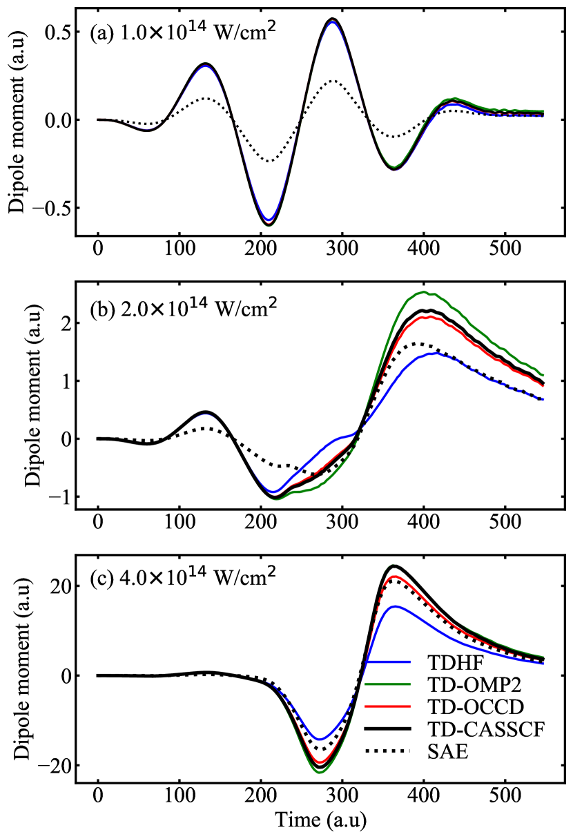
Figure 1: Time evolution of sign-flipped dipole moment $\langle z\rangle$ of Ar irradiated by a laser pulse with a wavelength of 1200 nm and a peak intensity of 1$\times$10¹⁴ W/cm² (a), 2$\times$10¹⁴ W/cm² (b) and 4$\times$10¹⁴ W/cm² (c), calculated with TDHF, TD-OMP2, TD-OCCD, TD-CASSCF, and SAE methods.

III.2 Ar in a strong laser field

We present numerical applications of the present method to Ar subject to an intense laser pulse linearly polarized in the $z$ direction. Calculations for intense long-wavelength laser fields are computationally demanding, thus serving as a good test for the newly implemented methods. The laser-electron interaction is introduced to the one-body part of the electronic Hamiltonian within the dipole approximation in the velocity gauge,

$$h(\bm{r},\bm{p})=\frac{1}{2}|\bm{p}|^{2}-\frac{Z}{|\bm{r}|}+A(t)p_{z},$$ (28)

where $Z(=18)$ is the atomic number, $A(t)=-\int^{t}E(t^{\prime})dt^{\prime}$ is the vector potential, with $E(t)$ being the laser electric field. While our method is gauge-invariant, we obtain faster convergence with the velocity gauge for the case of intense long-wavelength laser pulses sato2016time ; orimo2018implementation .

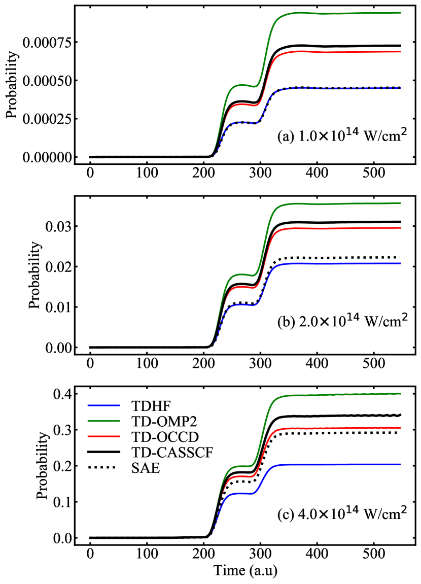
Figure 2: Time evolution of single ionization probability of Ar irradiated by a laser pulse with a wavelength of 1200 nm and a peak intensity of 1$\times$10¹⁴ W/cm² (a), 2$\times$10¹⁴ W/cm² (b) and 4$\times$10¹⁴ W/cm² (c) calculated with TDHF, TD-OMP2, TD-OCCD, TD-CASSCF, and SAE methods.

The laser electric field is of the following form

$$E(t)=E_{0}\,{\text{sin}}(\omega_{0}t)\,{\text{sin}}^{2}\left(\pi\frac{t}{3T}\right),$$ (29)

for $0\leq t\leq 3T$, and $E(T)=0$ otherwise, with the central wavelength $\lambda=2\pi/\omega_{0}=1200$ nm, the period $T=2\pi/\omega_{0}\sim 4.00$ fs, and the peak intensity $I_{0}=E_{0}^{2}$. We have considered three different intensities of 1, 2, and 4 $\times$10¹⁴ W/cm² for Ar.

The spherical finite-element discrete variable representation (FEDVR) basis sato2016time ; orimo2018implementation is used in our implementation. The convergence with respect to the maximum angular momentum $l_{\text{max}}$ is checked at the TDHF level, and $l_{\text{max}}$ is set to 72. The radial coordinate $r$ is discretized by FEDVR consisting of 78 finite elements with 23 DVR functions each, to support $0<r<R_{\text{max}}=300$. A ${\cos^{\frac{1}{4}}}$ mask function is switched on at 240 to avoid reflection from the boundary. Fourth-order exponential Runge-Kutta integrator exponential_integrator is used to propagate equations of motions with 20000 time steps per optical cycle. The simulations are continued after the end of pulse for further 6000 time steps.

For ab initio TDHF, TD-OMP2, TD-OCCD, and TD-CASSCF methods, the $1s2s2p$ core is kept frozen, and the dynamics of remaining eight electrons are actively taken into account with four (TDHF) or thirteen (TD-OMP2, TD-OCCD, and TD-CASSCF) active orbitals. The SAE method first diagonalizes the following effective HamiltonianMuller:1998 ; Schiessl:2006

$$h_{\rm eff}=\frac{1}{2}|\bm{p}|^{2}+V_{\rm eff}(|\bm{r}|),$$ (30)

on the FEDVR basis, where the effective potential $V_{\rm eff}(r)$ is taken to beMuller:1998 ; Schiessl:2006

$$V_{\rm eff}(r)=-\frac{1}{r}\left\{1+Ae^{-r}+(Z-1-A)e^{-Br}\right\},$$ (31)

with $A=5.4$ and $B=3.682$ for Ar Schiessl:2006 . This potential correctly supports $1s$, $2s$, $2p$, $3s$, and $3p$ bound orbitals, with the $3p$ orbital energy of -15.82 eV with the present FEDVR basis. After obtaining the ground state, we solve the effective one-electron Schrödinger equation,

$$i\frac{d}{dt}|\chi\rangle=\hat{Q}\left\{h_{\rm eff}+A(t)p_{z}\right\}|\chi\rangle,$$ (32)

starting from the $3p_{0}$ orbital. The projector $\hat{Q}=1-\sum_{j}|\phi_{j}\rangle\langle\phi_{j}|$, with $\phi_{j}$ running over $1s$, $2s$, $2p$, $3s$, and $3p_{\pm}$ orbitals [multiplied by the gauge factor $e^{-iA(t)z}$], keeps $\chi(t)$ orthonormal to the inner shell orbitals.

In Fig. 1, we plot the time evolution of the sign-flipped dipole moment $\langle z\rangle$ evaluated as a trace $\langle z\rangle=\langle\psi_{p}|\hat{z}|\psi_{q}\rangle\rho^{q}_{p}$ for ab initio methods and $\langle z\rangle=\langle\chi|z|\chi\rangle$ for SAE. We compare the TD-OMP2 results with SAE, TDHF, TD-OCCD, and TD-CASSCF ones. Within the same active space, TD-CASSCF produces highly accurate results, useful for performance analysis of the TD-OMP2 method.

The lowest ($1.0\times 10^{14}$ W/cm²) and highest ($4.0\times 10^{14}$ W/cm²) intensity cases characterize the dynamics with small and substantial amount of ionization, respectively (Fig. 2 below). The SAE approximation is knownkrause1992jl ; kulander1987time ; Muller:1998 to work better for the latter case, where the dynamics is dominated by tunneling ionization of the single, most weakly bound electron (one of the $3p_{0}$ electrons in the present case). It is not well suited for describing the former case dominated by collective bound dynamics. On the other hand, TDHF serves as the reference multielectron method without the (Coulomb) correlation by definition, and provides a qualitatively correct description of the bound dynamics. It, however, fails to accurately describe cases with sizable tunneling ionization. (See, e.g, Ref. 67 and references therein.) These trends of SAE and TDHF methods are well confirmed in the performance comparison to the reference TD-CASSCF method in Figs. 1 and 2.

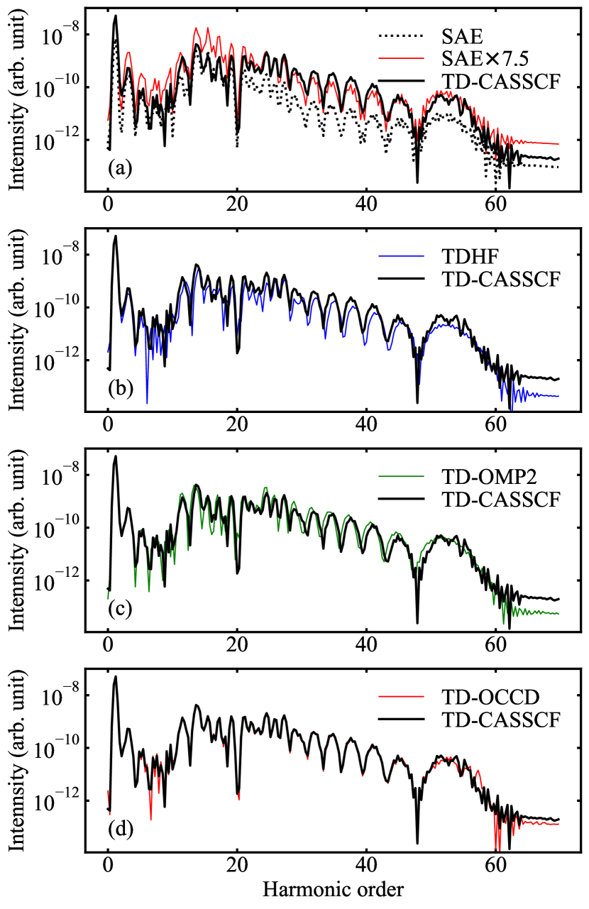
Figure 3: The HHG spectra from Ar irradiated by a laser pulse with a wavelength of 1200 nm and a peak intensity of 1$\times$10¹⁴ W/cm². Comparison of the results of SAE (a), TDHF (b), TD-OMP2 (c), and TD-OCCD (d) methods with that of TD-CASSCF.

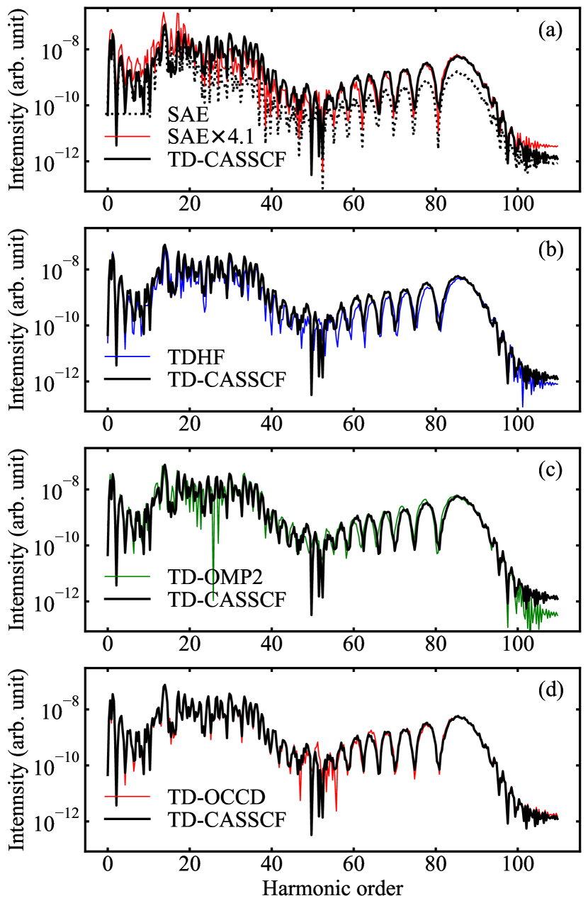
Figure 4: The HHG spectra from Ar irradiated by a laser pulse with a wavelength of 1200 nm and a peak intensity of 2$\times$10¹⁴ W/cm². Comparison of the results of SAE (a), TDHF (b), TD-OMP2 (c), and TD-OCCD (d) methods with that of TD-CASSCF.

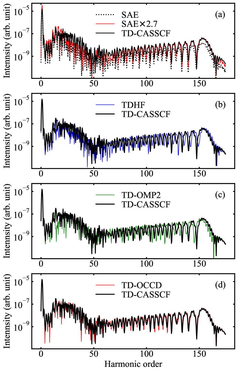
Figure 5: The HHG spectra from Ar irradiated by a laser pulse with a wavelength of 1200 nm and a peak intensity of 4$\times$10¹⁴ W/cm². Comparison of the results of SAE (a), TDHF (b), TD-OMP2 (c), and TD-OCCD (d) methods with that of TD-CASSCF.

As seen in Fig. 1-(a), at the lowest intensity of $10^{14}\,{\rm W/cm}^{2}$ all the methods except for SAE produce similar results. The TD-OCCD produces virtually the identical result with the TD-CASSCF, whereas TD-OMP2 slightly overestimates, and TDHF underestimates, considering TD-CASSCF as the benchmark. With increase in intensity, the difference among the methods become more prominent. While all the methods except for SAE give similar results in the early stage, TD-OMP2 and TDHF start to overestimate and underestimate, respectively, with the progress of tunneling ionization (Fig. 2). In general, the performance of the TD-OMP2 method is better than TDHF and SAE due to consideration at least a part of the electron correlation. It is noticed that the TD-OMP2 dipole moment agrees better with the TD-CASSCF one for the highest intensity [Fig. 1-(c)] than for the intermediate one [Fig. 1-(b)], which might indicate that the latter case, with both sizable ionization and nontrivial correlation effects coexisting, is theoretically more challenging.

The general trends in Fig. 1 are also found in the single ionization probability (Fig. 2), evaluated as the probability of finding an electron outside a sphere of 20 a.u. radius. Again, we see a systematic overestimation by TD-OMP2 and underestimation by TDHF in comparison to the TD-CASSCF result; the performance of TD-OMP2 is better than that of TDHF and SAE, except for the highest intensity case, where the SAE result is as accurate as the TD-OCCD one.

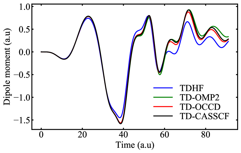
Figure 6: Time evolution of sign-flipped dipole moment $\langle z\rangle$ of Ar irradiated by a laser pulse with a wavelength of 200 nm and a peak intensity of 4$\times$10¹⁴ W/cm², calculated with TDHF, TD-OMP2, TD-OCCD, and TD-CASSCF methods.

Table 2: Comparison of the CPU time${}^{\text{a}}$ (in second) spent for the evaluation of the $T_{2}$ equation, $\Lambda_{2}$ equation, and 2RDM for TD-OCCD and TD-OMP2 methods

TD-OCCD				TD-OMP2
T2	$\Lambda_{2}$	2RDM		T2	$\Lambda_{2}$	2RDM
40.8	55.5	109.5		1.11	-	0.25

In Figs. 3–5 we compare HHG spectra, calculated as the modulus squared of the Fourier transform of the expectation value of the dipole acceleration, which, in turn, is obtained with a modified Ehrenfest expressionsato2016time . All ab initio methods reproduce the HHG spectra relatively well, including an experimentally observed characteristic dip around the 52nd order ($\sim 54$ eV) at $2\times$ and $4\times 10^{14}\,{\rm W/cm}^{2}$ related to the Cooper minimum of the photoionization spectrumPhysRevLett.102.103901 at the same energy. However, TDHF systematically underestimates and fails to reproduce fine details. The SAE method severely underestimates the HHG yields, although the overall shape of the HHG spectrum is well reproduced, and an intensity-dependent scaling brings the spectral intensity at the higher plateau close to that of TD-CASSCF, especially for the highest intensity. The agreement with the TD-CASSCF results is much better for the TD-OCCD method, which contains nonlinear terms in the amplitude equations, then followed by TD-OMP2 with slight overestimation. This trend is consistent with the capability of each method to treat the electron correlation.

In order to investigate the performance of TD-OMP2 method for shorter wavelengths, where electrons not only in the highest-occupied but also in the inner-shell orbitals are driven by the laser, we consider a shorter wavelength of 200 nm with an intensity of 4$\times$10¹⁴ W/cm². All the other simulation parameters are identical to those given above. The obtained time evolution of the dipole moment (Fig. 6) shows a slight overestimation of the oscillation amplitude by TD-OMP2 and underestimation by TDHF compared to the TD-CASSCF result as in the case for the longer wavelength. It is encouraging, however, that the TD-OMP2 result is much closer to the TD-CASSCF one for the shorter wavelength, which is more sensitive to the treatment of correlation effects.

It is worth noting that, for an intensity as high as $4\times 10^{14}\,{\rm W/cm}^{2}$, the TD-OMP2 simulation completed stably. This should be the direct consequence of full inclusion of the laser-electron interaction in the zeroth-order Hamiltonian and the orbital optimization (propagation) according to the time-dependent variational principle based on the total (up to second-order) Lagrangian, which keeps the instantaneous perturbation $\hat{H}^{(1)}=\hat{H}-\hat{f}$ relatively small in the present simulation.

Finally, the computational cost of different parts of TD-OMP2 and TD-OCCD methods are compared in Table 2 for the same computational condition as in Fig. 3 (c). The evaluation of $T_{2}$ equation, $\Lambda_{2}$ equation, and 2RDM all scale as $N^{6}$ for the TD-OCCD method. On the other hand, for the TD-OMP2 method, the evaluation of $T_{2}$ equation scales as $N^{5}$, and we do not need a separate solution for $\Lambda_{2}$, as it is just the complex conjugate of $T_{2}$. The greatest time saving for the TD-OMP2 method comes from the evaluation of 2RDM since it scales as $N^{4}$, and does not involve any operator products. Overall, TD-OMP2 achieves a significant cost reduction compared to TD-OCCD, making it an attractive choice for simulations involving larger chemical systems.

IV conclusion

We have successfully implemented the TD-OMP2 method for the real-time simulations of laser-induced dynamics in relatively large chemical systems. The TD-OMP2 method retains the size-extensivity and gauge-invariance of TD-OCC, and is computationally much more efficient than the full TD-OCCD method. As a first numerical test, we have applied the method to the ground state of BH and the laser-driven dynamics of Ar. The imaginary time relaxation for BH obtains the identical ground-state energies with those by the stationary theory, which indicates the correctness of the implementation. The performance of the present method is numerically investigated in comparison to SAE, TDHF, TD-OCCD, and TD-CASSCF methods for the case of laser-driven Ar. The results suggest a decent performance with a consistent overestimation of the correlation effect in such highly nonlinear phenomena. Remarkably, the TD-OMP2 method is stable and does not breakdown even in the presence of strong laser-electron interaction, thanks to the nonperturbative inclusion of external fields and time-dependent orbital optimization. Further assessment of the TD-OMP2 method for different systems and severer simulation conditions (e.g, with higher-intensity and/or longer-wavelength lasers) will be reported elsewhere.

DATA AVAILABLITY

The data that support the findings of this study are available from the corresponding author upon reasonable request.

References

- (1) P. á. Corkum and F. Krausz, Nature physics 3, 381 (2007).
- (2) F. Krausz and M. Ivanov, Reviews of Modern Physics 81, 163 (2009).
- (3) J. Itatani et al., Nature 432, 867 (2004).
- (4) E. Goulielmakis et al., Nature 466, 739 (2010).
- (5) G. Sansone et al., Nature 465, 763 (2010).
- (6) M. Schultze et al., Science 328, 1658 (2010).
- (7) K. Klünder et al., Physical Review Letters 106, 143002 (2011).
- (8) L. Belshaw et al., The journal of physical chemistry letters 3, 3751 (2012).
- (9) F. Calegari et al., Science 346, 336 (2014).
- (10) O. Smirnova et al., Nature 460, 972 (2009).
- (11) P. Antoine, A. L’huillier, and M. Lewenstein, Physical Review Letters 77, 1234 (1996).
- (12) K. L. Ishikawa and T. Sato, IEEE Journal of Selected Topics in Quantum Electronics 21, 1 (2015).
- (13) I. Tikhomirov, T. Sato, and K. L. Ishikawa, Physical review letters 118, 203202 (2017).
- (14) Y. Li, T. Sato, and K. L. Ishikawa, Phys. Rev. A 99, 043401 (2019).
- (15) S. Pabst and R. Santra, Phys. Rev. Lett. 111, 233005 (2013).
- (16) J. S. Parker, E. S. Smyth, and K. T. Taylor, Journal of Physics B: Atomic, Molecular and Optical Physics 31, L571 (1998).
- (17) J. S. Parker et al., Journal of Physics B: Atomic, Molecular and Optical Physics 33, L239 (2000).
- (18) M. Pindzola and F. Robicheaux, Physical Review A 57, 318 (1998).
- (19) S. Laulan and H. Bachau, Physical Review A 68, 013409 (2003).
- (20) K. L. Ishikawa and K. Midorikawa, Physical Review A 72, 013407 (2005).
- (21) J. Feist et al., Physical review letters 103, 063002 (2009).
- (22) K. L. Ishikawa and K. Ueda, Physical review letters 108, 033003 (2012).
- (23) S. Sukiasyan, K. L. Ishikawa, and M. Ivanov, Physical Review A 86, 033423 (2012).
- (24) W. Vanroose, D. A. Horner, F. Martin, T. N. Rescigno, and C. W. McCurdy, Physical Review A 74, 052702 (2006).
- (25) D. A. Horner et al., Physical review letters 101, 183002 (2008).
- (26) J. Krause, Phys. Rev. Lett. 68, 3535 (1992).
- (27) K. C. Kulander, Physical Review A 36, 2726 (1987).
- (28) J. Caillat et al., Physical review A 71, 012712 (2005).
- (29) T. Kato and H. Kono, Chemical physics letters 392, 533 (2004).
- (30) M. Nest, T. Klamroth, and P. Saalfrank, The Journal of chemical physics 122, 124102 (2005).
- (31) D. J. Haxton, K. V. Lawler, and C. W. McCurdy, Physical Review A 83, 063416 (2011).
- (32) D. Hochstuhl and M. Bonitz, The Journal of chemical physics 134, 084106 (2011).
- (33) T. Sato and K. L. Ishikawa, Physical Review A 88, 023402 (2013).
- (34) T. Sato et al., Physical Review A 94, 023405 (2016).
- (35) H. Miyagi and L. B. Madsen, Physical Review A 87, 062511 (2013).
- (36) H. Miyagi and L. B. Madsen, Physical Review A 89, 063416 (2014).
- (37) D. J. Haxton and C. W. McCurdy, Physical Review A 91, 012509 (2015).
- (38) T. Sato and K. L. Ishikawa, Physical Review A 91, 023417 (2015).
- (39) J. J. Omiste, W. Li, and L. B. Madsen, Phys. Rev. A 95, 053422 (2017).
- (40) Y. Orimo, T. Sato, A. Scrinzi, and K. L. Ishikawa, Physical Review A 97, 023423 (2018).
- (41) R. Anzaki, T. Sato, and K. L. Ishikawa, Phys. Chem. Chem. Phys. 19, 22008 (2017).
- (42) A. U. J. Lode, C. Lévêque, L. B. Madsen, A. I. Streltsov, and O. E. Alon, Rev. Mod. Phys. 92, 011001 (2020).
- (43) T. Sato, H. Pathak, Y. Orimo, and K. L. Ishikawa, The Journal of chemical physics 148, 051101 (2018).
- (44) C. D. Sherrill, A. I. Krylov, E. F. Byrd, and M. Head-Gordon, The Journal of chemical physics 109, 4171 (1998).
- (45) A. I. Krylov, C. D. Sherrill, E. F. Byrd, and M. Head-Gordon, The Journal of chemical physics 109, 10669 (1998).
- (46) S. Kvaal, The Journal of chemical physics 136, 194109 (2012).
- (47) J. Arponen, Annals of Physics 151, 311 (1983).
- (48) H. Pathak, T. Sato, and K. L. Ishikawa, arXiv:2001.02206 .
- (49) W. Meyer, International Journal of Quantum Chemistry 5, 341 (1971).
- (50) R. Ahlrichs, P. Scharf, and C. Ehrhardt, The Journal of Chemical Physics 82, 890 (1985).
- (51) F. Wennmohs and F. Neese, Chemical Physics 343, 217 (2008).
- (52) F. Neese, F. Wennmohs, and A. Hansen, The Journal of chemical physics 130, 114108 (2009).
- (53) C. Kollmar and F. Neese, Molecular Physics 108, 2449 (2010).
- (54) J.-P. Malrieu, H. Zhang, and J. Ma, Chemical Physics Letters 493, 179 (2010).
- (55) J. Čížek, The Journal of Chemical Physics 45, 4256 (1966).
- (56) R. J. Bartlett, Annual Review of Physical Chemistry 32, 359 (1981).
- (57) U. Bozkaya, J. M. Turney, Y. Yamaguchi, H. F. Schaefer III, and C. D. Sherrill, The Journal of chemical physics 135, 104103 (2011).
- (58) L. Adamowicz and R. J. Bartlett, The Journal of chemical physics 86, 6314 (1987).
- (59) F. Neese, T. Schwabe, S. Kossmann, B. Schirmer, and S. Grimme, Journal of chemical theory and computation 5, 3060 (2009).
- (60) U. Bozkaya, The Journal of chemical physics 135, 224103 (2011).
- (61) J. M. Turney et al., Wiley Interdisciplinary Reviews: Computational Molecular Science 2, 556 (2012).
- (62) M. Frisch et al., Gaussian 09, revision d. 01, 2009.
- (63) R. Harrison and N. Handy, Chemical Physics Letters 95, 386 (1983).
- (64) M. Hochbruck and A. Ostermann, Acta Numerica 19, 209 (2010).
- (65) H. G. Muller and F. C. Kooiman, Phys. Rev. Lett 81, 1207 (1998).
- (66) K. Schiessl, E. Persson, A. Scrinzi, and J. Burgdörfer, Physical Review A 74, 053412 (2006).
- (67) T. Sato and K. L. Ishikawa, J. Phys. B: At. Mol. Opt. Phys. 47, 204031 (2014).
- (68) H. J. Wörner, H. Niikura, J. B. Bertrand, P. B. Corkum, and D. M. Villeneuve, Phys. Rev. Lett. 102, 103901 (2009).