Event-Triggered Consensus of Homogeneous and Heterogeneous Multi-Agent Systems with Jointly Connected Switching Topologies

Abstract

This paper investigates the distributed event-based consensus problem of switching networks satisfying the jointly connected condition. Both the state consensus of homogeneous linear networks and output consensus of heterogeneous networks are studied. Two kinds of event-based protocols based on local sampled information are designed, without the need to solve any matrix equation or inequality. Theoretical analysis indicates that the proposed event-based protocols guarantee the achievement of consensus and the exclusion of Zeno behaviors for jointly connected undirected switching graphs. These protocols, relying on no global knowledge of the network topology and independent of switching rules, can be devised and utilized in a completely distributed manner. They are able to avoid continuous information exchanges for either controllers’ updating or triggering functions’ monitoring, which ensures the feasibility of the presented protocols.

I introduction

Event-driven coordination has been widely studied and started maturing to soon stand alone in the control area in the last decade [1, 2, 3, 4, 5, 6, 7, 8, 9]. Compared to classic continuous control approaches, event-based control has numerous advantages especially in enhancing control efficiency, such as avoiding continuously updating controllers and continuous communications among neighboring agents. The latter advantage is particularly evident when we focus on Internet of Things and other large-scale networks where the cyber operations, including processing, storage, and communication, must be viewed as a scare, globally shared resource [10]. Due to these practical considerations, it is not surprising that so many researchers are interested in event-triggered control and present plenty of results. Applying event-driven control in networked systems poses some new challenges that do not exist in either area alone [10]. As pointed out in [10], researchers must consider how to deal with the natural asynchronism introduced into the systems and how to rule out the Zeno behavior. Another challenge is that the separation principle cannot be used for event-triggered control systems anymore [11].

Existing works have presented a large number of insights into general coordination of networked systems with event-triggered mechanisms. As a specific case study, event-triggered consensus is a longstanding area of research in multi-agent systems; see the references [12, 13, 14, 15, 16, 17, 18, 19]. Many survey papers about event-driven control were published, such as [10, 20, 21, 22]. Generally speaking, existing consensus protocols are designed for either state consensus of homogeneous networks or output consensus of heterogeneous networks. Noting that for heterogeneous networks, where even the dimensions of states may be different, output consensus is a more meaningful topic than state consensus.

In the field of state consensus of homogeneous networks, [23, 24, 25] presented event-based protocols for single-integrator agents under undirected graphs. To remove the limitation that continuous information was still required in triggering functions of early works, [26] proposed triggering functions only based on discrete sampled information. The authors of [27, 28, 29] presented event-driven consensus algorithms for general linear networks. Reference [30] studied the event-driven consensus using output feedback control. The event-based consensus control problem with external disturbances was studied in [31, 32, 33]. Event-driven output consensus of heterogeneous networks was studied in [34, 35]. The authors of [36] studied event-based cooperative output regulation problem of heterogeneous networks.

It should be noted that the proposed protocols in the above works were only designed for fixed and connected topologies. However, in many practical cases, the topologies may be switching [37, 38, 39, 40] and do not satisfy the connected condition. In [41], the authors proposed an event-driven protocol for networks with switching communication graphs. One limitation of the protocol in [41], that the triggering functions were designed based on continuous information, may limit its practical applicability. To avoid continuous interagent communication, [42] proposed decentralized event-based controllers for leader-follower networks under fixed or switching graphs. The results of [42] relied on an assumption that the (switching) topology is connected at every moment, which was not always satisfied for general switching topologies. In particular, there were even no any connections among agents at some special instants. This assumption was removed by the authors of [43, 44], in which similar problems were considered. The designs of the protocols proposed in [43, 44], nevertheless, required to solve two coupled inequalities, while the existence of the solution is unclear in general cases. The switching nature of topologies coupled with event-triggered communications makes it troublesome to propose distributed consensus algorithms, and the existence of heterogeneity renders the task for heterogeneous networks more challenging. How to devise event-triggered consensus algorithms for linear homogeneous (or heterogeneous) networks with general switching topologies needs further investigation.

In the current paper, we study the event-driven consensus control problems with switching graphs, including state consensus of homogeneous linear networks and output consensus of heterogeneous linear networks. For the homogeneous case, we present an event-based protocol, composed of controllers and triggering rules. Under this protocol, communications will not take place until the topology switches or the designed measurement error exceeds an appropriate threshold. It is shown that state consensus is achieved and Zeno behaviors are ruled out. The protocol can be explicitly constructed and do not need to solve any matrix equation or inequality. We also consider event-based output consensus of heterogeneous networks with switching topologies and an exogenous signal that can be viewed as a reference input or an external disturbance. For this problem, we first devise distributed observers to estimate the exogenous signal and then propose local control inputs.

The main contributions of this paper are listed as follows. We have solved both the event-based state consensus control problem of homogeneous networks and the event-based output consensus control problem of heterogeneous networks. Different from existing related papers, the proposed event-triggered protocols of this paper can be used for any switching graphs satisfying the jointly connected condition, including fixed graphs as a special case. The proposed protocols, requiring no global information associated with the whole network and independent of the switching rules, can be devised and utilized in a completely distributed manner. The Zeno behavior can be excluded at any finite time by showing that the interval between any different triggering instants is not less than a strictly positive value. This feature ensures the feasibility of the above protocols when they are implemented on practical systems.

Here is the outline of this paper. In Section II, we consider the event-driven state consensus of homogeneous networks. We then study event-based output consensus of heterogeneous networks in Section III. Numerical simulations and conclusions are presented in Sections IV and V, respectively.

II event-based state consensus of homogeneous multi-agent systems

II-A Problem Formulation

In this section, we consider $N$ homogeneous linear agents, whose dynamics satisfy

$$\dot{x}_{i}=Ax_{i}+Bu_{i},~{}i=1,\cdots,N,$$ (1)

where $x_{i}\in\mathbf{R}^{n}$ denotes the state, $u_{i}\in\mathbf{R}^{p}$ represents the control input, and $A\in\mathbf{R}^{n\times n}$, $B\in\mathbf{R}^{n\times p}$ are constant matrices.

Assumption 1

The pair $(A,B)$ is stabilizable and $A$ is neutrally stable .

Denote $\theta:~{}[0,+\infty)\rightarrow\Theta$ as a switching signal with a positive dwelling time $\tau$. Let $\mathcal{G}_{\theta(t)}\triangleq(\mathcal{V},\mathcal{E}_{\theta(t)})$ represent an undirected graph among the $N$ agents, where $\mathcal{V}=\{1,\cdots,N\}$ and $\mathcal{E}_{\theta(t)}\subseteq\mathcal{V}\times\mathcal{V}$ denote the sets of nodes and edges, respectively. Consider an infinite time sequence composed of nonempty, bounded, and contiguous intervals $[\bar{t}_{0},\bar{t}_{1})$, $\cdots$, $[\bar{t}_{k},\bar{t}_{k+1})$, $\cdots$, with $\bar{t}_{0}=0$. Suppose $\bar{t}_{k+1}-\bar{t}_{k}\leq T$ with $T$ being some positive constant and during each interval $[\bar{t}_{k},\bar{t}_{k+1})$, there are finite nonoverlapping subintervals

$$[\bar{t}_{k}^{0},\bar{t}_{k}^{1}),[\bar{t}_{k}^{1},\bar{t}_{k}^{2}),\cdots,[\bar{t}_{k}^{m_{k}-1},\bar{t}_{k}^{m_{k}}),~{}\bar{t}_{k}=\bar{t}_{k}^{0},~{}\bar{t}_{k+1}=\bar{t}_{k}^{m},$$

satisfying $\bar{t}_{k}^{j+1}-\bar{t}_{k}^{j}\geq\tau$, $j=0,1,\cdots,m_{k}-1$. And $\mathcal{G}_{\theta(t)}$ is fixed during each subinterval. An edge of $\mathcal{E}_{\theta(t)}$ is composed of two distinct nodes of $\mathcal{V}$. If $(i,j)\in\mathcal{E}_{\theta(t)}$, $i$ and $j$ are neighbors under graph $\mathcal{G}_{\theta(t)}$. An undirected path between nodes $i$ and $j$ is denoted as $({i_{1}},{i_{2}})$, $({i_{2}},{i_{3}})$, $\cdots$, $({i_{q}},j)$. Denote the adjacency matrix of graph $\mathcal{G}_{\theta(t)}$ by $\mathcal{A}(t)=[a_{ij}(t)]\in\mathbf{R}^{N\times N}$, where $a_{ii}(t)=0$, $a_{ij}(t)=1$ if $(j,i)\in\mathcal{E}_{\theta(t)}$ and $a_{ij}(t)=0$ otherwise. Denote the Laplacian matrix $\mathcal{L}_{\theta(t)}=[l_{ij}(t)]\in\mathbf{R}^{N\times N}$ of $\mathcal{G}_{\theta}$ by $l_{ii}(t)=\sum_{j=1}^{N}{a_{ij}(t)}$ and $l_{ij}(t)=-a_{ij}(t)$, $i\neq j$. Define the degree as $d_{i}(t)=l_{ii}(t)$, $i\in\mathcal{V}$. Then, define $\bigcup_{t\in[\bar{t}_{k},\bar{t}_{k+1})}\mathcal{G}_{\theta(t)}$ as a union graph in the collection for time $t$ from $\bar{t}_{k}$ to $\bar{t}_{k+1}$.

Assumption 2

The undirected graph $\mathcal{G}_{\theta(t)}$ of the $N$ agents is jointly connected, i.e., $\bigcup_{t\in[\bar{t}_{k},\bar{t}_{k+1})}\mathcal{G}_{\theta(t)}$ is connected.

The objective here is to present distributed event-based algorithms under which all subsystems described by (1) converge to a common state trajectory and Zeno behaviors can be eliminated.

Instead of using agents’ actual states, define the state estimate as $\tilde{x}_{i}(t)\triangleq e^{A(t-t_{k}^{i})}x_{i}(t_{k}^{i})$, $\forall t\in[t_{k}^{i},t_{k+1}^{i})$, $i=1,\cdots,N$, where $t_{k}^{i}$ denotes the $k$-th event instant of agent $i$. The event instants $t_{0}^{i}$, $t_{1}^{i}$, $\cdots$, are determined by the triggering function to be designed later. Using the relative state estimates of neighboring agents, we present a distributed event-based controller as:

$$u_{i}(t)=cG\sum_{j=1}^{N}{a_{ij}(t)(\tilde{x}_{i}-\tilde{x}_{j})},~{}i\in\mathcal{V},$$ (2)

where $c>0$ and $G\in\mathbf{R}^{p\times n}$ are design parameters.

Define $\xi=[\xi_{1}^{T},\cdots,\xi_{N}^{T}]^{T}$ and $\tilde{\xi}=[\tilde{\xi}_{1}^{T},\cdots,\tilde{\xi}_{N}^{T}]^{T}$ with $\xi_{i}\triangleq x_{i}-\frac{1}{N}\sum_{j=1}^{N}{x_{j}}$ and $\tilde{\xi}_{i}\triangleq\tilde{x}_{i}-\frac{1}{N}\sum_{j=1}^{N}{\tilde{x}_{j}}$, $i=1,\cdots,N$. Letting $x\triangleq[x_{1}^{T},\cdots,x_{N}^{T}]^{T}$ gives $\xi=(M\otimes I_{n})x$ and $\tilde{\xi}=(M\otimes I_{n})\tilde{x}$, where $M=I_{N}-\frac{1}{N}\mathbf{1}_{N}\mathbf{1}_{N}^{T}$. Noting that $\xi=0$ if and only if $x_{1}=\cdots=x_{N}$, we call $\xi$ the consensus error, whose dynamics is given by

$$\dot{\xi} =(I_{N}\otimes A)\xi+(c\mathcal{L}_{\theta}\otimes BG)\tilde{\xi}.$$ (3)

Note that the control law (2) is only updated according to the information received at the latest event time instant, defined by

$$t_{k+1}^{i} \triangleq\mathrm{inf}\{t>t_{k}^{i}~{}|~{}f_{i}(t)\geq 0~{}\mathrm{or}~{}a_{ij}(t)\neq a_{ij}(t_{k}^{i})$$ (4)

$$~{}~{}~{}~{}~{}~{}~{}~{}\mathrm{for~{}some}~{}j\in\mathcal{V}\},$$

where $t_{0}^{i}\triangleq 0$ and $f_{i}(t)$ is the triggering function defined as follows:

$$f_{i}(t) =4d_{i}(t)\|G\|^{2}\|e_{i}\|^{2}-\delta\sum_{j=1}^{N}{a_{ij}(t)\|G(\tilde{x}_{i}-\tilde{x}_{j})\|^{2}}$$ (5)

$$\quad-\mu e^{-\nu t},~{}i=1,\cdots,N,$$

with $\delta$, $\mu$, $\nu$ being positive constants, and $e_{i}\triangleq\tilde{x}_{i}-x_{i}$ being the measurement error. Once $f_{i}$ triggers, agent $i$ broadcasts its current state to neighbors. The controllers (2) of $i$ and its neighbors update immediately, and $e_{i}(t)$ resets at the same time.

II-B Event-Based Consensus Conditions

Since $A$ is neutrally stable, in light of Lemmas 22 and 23 of [4], we can choose $E\in\mathbf{R}^{{n_{1}}\times n}$ and $F\in\mathbf{R}^{{(n-n_{1})}\times n}$ satisfying

$$\begin{bmatrix}E\\ F\end{bmatrix}A\begin{bmatrix}E\\ F\end{bmatrix}^{-1}=\begin{bmatrix}X&0\\ 0&Y\end{bmatrix},$$

where $X\in\mathbf{R}^{{n_{1}}\times{n_{1}}}$ is skew-symmetric and $Y\in\mathbf{R}^{{(n-n_{1})}\times{(n-n_{1})}}$ is Hurwitz.

Remark 1

It should be pointed out that the matrices $E$ and $F$ can be derived by rendering the matrix $A$ into the real Jordan canonical form [45].

Choose $z=\left(I_{N}\otimes\begin{bmatrix}E\\ F\end{bmatrix}\right)\xi$ and $\tilde{z}=\left(I_{N}\otimes\begin{bmatrix}E\\ F\end{bmatrix}\right)\tilde{\xi}$. The derivative of $z$ is given by

$$\dot{z}=\left(I_{N}\otimes\begin{bmatrix}X&0\\ 0&Y\end{bmatrix}\right)z+\left(c\mathcal{L}\otimes\begin{bmatrix}E\\ F\end{bmatrix}BG\begin{bmatrix}E\\ F\end{bmatrix}^{-1}\right)\tilde{z}.$$ (6)

Let $H=EB$. According to Assumption 1, $(X,H)$ is controllable. Choose $E^{+}\in\mathbf{R}^{n\times{n_{1}}}$ and $F^{+}\in\mathbf{R}^{n\times{(n-n_{1})}}$ satisfying $\begin{bmatrix}E^{+}&F^{+}\end{bmatrix}=\begin{bmatrix}E\\ F\end{bmatrix}^{-1}$, with $EE^{+}=I$, $FF^{+}=I$, $FE^{+}=0$, and $EF^{+}=0$. Letting $G=-B^{T}E^{T}E$, then we have

$$\dot{z}=\left(I_{N}\otimes\begin{bmatrix}X&0\\ 0&Y\end{bmatrix}\right)z-\left(c\mathcal{L}_{\theta}\otimes\begin{bmatrix}EBB^{T}E^{T}&0\\ FBB^{T}E^{T}&0\end{bmatrix}\right)\tilde{z}.$$ (7)

Define $z_{I}=(I_{N}\otimes E)\xi$, $\tilde{z}_{I}=(I_{N}\otimes E)\tilde{\xi}$, $z_{II}=(I_{N}\otimes F)\xi$ and $\tilde{z}_{II}=(I_{N}\otimes F)\tilde{\xi}$. Rewrite (7) as

$$\dot{z}_{I}=(I_{N}\otimes X)z_{I}-(c\mathcal{L}_{\theta}\otimes HH^{T})\tilde{z}_{I},$$ (-1)

$$\dot{z}_{II}=(I_{N}\otimes Y)z_{II}-(c\mathcal{L}_{\theta}\otimes FBB^{T}E^{T})\tilde{z}_{I}.$$ (-2)

Lemma 1

(Cauchy’s Convergence Criterion [43]) The sequence $V(\bar{t}_{k})$, $k=0,1,2,\cdots$ converges if and only if for $\forall\varepsilon>0$, $\exists M_{\varepsilon}\in\mathbf{Z}_{+}$ satisfying $\forall k>M_{\varepsilon}$, $\left|V(\bar{t}_{k+1})-V(\bar{t}_{k})\right|<\varepsilon$.

Lemma 2

(Barbalat’s Lemma [46]) If $\lim_{t\rightarrow\infty}g(t)=a$ ($a$ is bounded) and $g^{\prime\prime}(t)$ is also bounded, then $\lim_{t\rightarrow\infty}g^{\prime}(t)=0$.

Next, we introduce the main results of this section.

Theorem 1

State consensus of the homogeneous subsystems (1) is achieved under the event-driven algorithm composed of (2) and (5) with $c>0$, $0<\delta<1$, $\mu>0$, $\nu>0$, and $G=-B^{T}E^{T}E$ .

Proof 1

Let

$$V_{1}=\frac{1}{2}z_{I}^{T}z_{I}.$$ (9)

In light of (-1), differentiating $V_{1}$ with respect to $t$ gives

$$\dot{V}_{1} =\frac{1}{2}z_{I}^{T}[I_{N}\otimes(X+X^{T})]z_{I}-z_{I}^{T}(c\mathcal{L}_{\theta}\otimes HH^{T})\tilde{z}_{I}.$$ (10)

Since $X$ is skew-symmetric, $z_{I}^{T}[I_{N}\otimes(X+X^{T})]z_{I}=0$. Then, we have

$$\dot{V}_{1} =-\frac{1}{2}z_{I}^{T}(c\mathcal{L}_{\theta}\otimes HH^{T})z_{I}-\frac{1}{2}\tilde{z}_{I}^{T}(c\mathcal{L}_{\theta}\otimes HH^{T})\tilde{z}_{I}$$ (11)

$$\quad+\frac{1}{2}e^{T}(c\mathcal{L}_{\theta}\otimes G^{T}G)e.$$

Let

$$V_{2}=\frac{1}{2}z_{II}^{T}(I_{N}\otimes P)z_{II},$$ (12)

where $P$ satisfies

$$PY+Y^{T}P+2I=0.$$ (13)

In light of (-2), differentiating $V_{2}$ with respect to $t$ gives

$$\dot{V}_{2} =\frac{1}{2}z_{II}^{T}[I_{N}\otimes(PY+Y^{T}P)]z_{II}$$ (14)

$$\quad-z_{II}^{T}(c\mathcal{L}_{\theta}\otimes PFBB^{T}E^{T})\tilde{z}_{I}.$$

Using the Young’s Inequality [10] gives

$$\quad-z_{II}^{T}(c\mathcal{L}_{\theta}\otimes PFBB^{T}E^{T})\tilde{z}_{I}\leq\frac{1}{2}z_{II}^{T}z_{II}$$ (15)

$$+\frac{c^{2}\lambda_{N}(\mathcal{L}_{\theta})}{2}\tilde{z}_{I}^{T}(\mathcal{L}_{\theta}\otimes EBB^{T}F^{T}PPFBB^{T}E^{T})\tilde{z}_{I}$$

$$\leq\frac{1}{2}z_{II}^{T}z_{II}+\frac{c\alpha_{1}}{2}\tilde{x}^{T}(\mathcal{L}_{\theta}\otimes G^{T}G)\tilde{x},$$

where $\alpha_{1}=c\lambda_{N}(\mathcal{L})\|PFB\|^{2}$ and $\lambda_{N}(\mathcal{L})$ denotes the largest eigenvalue of $\mathcal{L}_{\theta(t)}$ for all $t>0$.

Construct the Lyapunov function candidate as

$$V_{3}=\frac{\alpha_{1}}{1-\delta}V_{1}+V_{2}.$$ (16)

Evidently, $V_{3}$ is positive definite, whose derivative is given by

$$\dot{V}_{3} \leq\frac{c\alpha_{1}}{2(1-\delta)}[-z_{I}^{T}(\mathcal{L}_{\theta}\otimes HH^{T})z_{I}$$ (17)

$$\quad+e^{T}(\mathcal{L}_{\theta}\otimes G^{T}G)e-\tilde{x}^{T}(\mathcal{L}_{\theta}\otimes G^{T}G)\tilde{x}]$$

$$\quad+\frac{1}{2}z_{II}^{T}[I_{N}\otimes(PY+Y^{T}P+I)]z_{II}$$

$$\quad+\frac{c\alpha_{1}}{2}\tilde{x}^{T}(\mathcal{L}_{\theta}\otimes G^{T}G)\tilde{x}$$

$$\leq-\alpha_{2}z_{I}^{T}(\mathcal{L}_{\theta}\otimes HH^{T})z_{I}-\frac{1}{2}z_{II}^{T}z_{II}$$

$$\quad+\alpha_{2}[e^{T}(\mathcal{L}_{\theta}\otimes G^{T}G)e-\delta\tilde{x}^{T}(\mathcal{L}_{\theta}\otimes G^{T}G)\tilde{x}],$$

where $\alpha_{2}=\frac{c\alpha_{1}}{2(1-\delta)}$. Because $a_{ij}(t)=a_{ji}(t)$, we have

$$e^{T}(\mathcal{L}_{\theta}\otimes G^{T}G)e =\sum_{i=1}^{N}\sum_{j=1}^{N}{a_{ij}(t)e_{i}^{T}G^{T}G(e_{i}-e_{j})}$$ (18)

$$\leq 2\sum_{i=1}^{N}\sum_{j=1}^{N}{a_{ij}(t)e_{i}^{T}G^{T}Ge_{i}}$$

$$\leq 2\sum_{i=1}^{N}{d_{i}(t)\|G\|^{2}\|e_{i}\|^{2}},$$

and

$$\quad\tilde{x}^{T}(\mathcal{L}_{\theta}\otimes G^{T}G)\tilde{x}$$ (19)

$$=\sum_{i=1}^{N}\sum_{j=1}^{N}{a_{ij}(t)\tilde{x}_{i}^{T}G^{T}G(\tilde{x}_{i}-\tilde{x}_{j})}$$

$$=\frac{1}{2}\sum_{i=1}^{N}\sum_{j=1}^{N}{a_{ij}(t)(\tilde{x}_{i}-\tilde{x}_{j})^{T}G^{T}G(\tilde{x}_{i}-\tilde{x}_{j})}$$

$$=\frac{1}{2}\sum_{i=1}^{N}\sum_{j=1}^{N}{a_{ij}(t)\|G(\tilde{x}_{i}-\tilde{x}_{j})\|^{2}}.$$

By substituting (5), (18), and (19) into (17), we have

$$\dot{V}_{3}\leq-\alpha_{2}z_{I}^{T}(\mathcal{L}_{\theta}\otimes HH^{T})z_{I}-\frac{1}{2}z_{II}^{T}z_{II}$$ (20)

$$+\frac{\alpha_{2}}{2}\sum_{i=1}^{N}\{4d_{i}(t)\|G\|^{2}\|e_{i}\|^{2}-\delta\sum_{j=1}^{N}a_{ij}(t)\|G(\tilde{x}_{i}-\tilde{x}_{j})\|^{2}\}$$

$$\leq-\alpha_{2}z_{I}^{T}(\mathcal{L}_{\theta}\otimes HH^{T})z_{I}-\frac{1}{2}z_{II}^{T}z_{II}+\frac{\mu\alpha_{2}N}{2}e^{-\nu t}.$$

Define $\tilde{V}_{3}(t)=V_{3}(t)+\frac{\mu\alpha_{2}N}{2\nu}e^{-\nu t}$. Then, we have

$$\dot{\tilde{V}}_{3} \leq-\alpha_{2}z_{I}^{T}(\mathcal{L}_{\theta}\otimes HH^{T})z_{I}-\frac{1}{2}z_{II}^{T}z_{II}.$$ (21)

Combining with $\dot{\tilde{V}}_{3}(t)\leq 0$ and $\tilde{V}_{3}(t)\geq 0$, we have $\tilde{V}_{3}$ is bounded and $\lim_{t\rightarrow+\infty}\tilde{V}_{3}(t)$ exists. Based on Lemma 1, for $\forall\varepsilon>0$, $\exists M_{\varepsilon}\in\mathbf{Z}_{+}$ satisfying $\forall k\geq M_{\varepsilon}$,

$$\left|\tilde{V}_{3}(\bar{t}_{k+1})-\tilde{V}_{3}(\bar{t}_{k})\right|<\varepsilon,$$

or

$$\left|\int_{\bar{t}_{k}}^{\bar{t}_{k+1}}\dot{\tilde{V}}_{3}(t)dt\right|<\varepsilon.$$

It follows that

$$\left|\int_{\bar{t}_{k}^{0}}^{\bar{t}_{k}^{1}}\dot{\tilde{V}}_{3}(t)dt\right|+\cdots+\left|\int_{\bar{t}_{k}^{m_{k}-1}}^{\bar{t}_{k}^{m_{k}}}\dot{\tilde{V}}_{3}(t)dt\right|<\varepsilon.$$ (22)

In light of (21), for each subinterval $[\bar{t}_{k}^{j},\bar{t}_{k}^{j+1})$, $j=0,1,\cdots,m_{k}-1$, we have

$$\left|\int_{\bar{t}_{k}^{j}}^{\bar{t}_{k}^{j+1}}\dot{\tilde{V}}_{3}(t)dt\right| \geq\alpha_{2}\int_{\bar{t}_{k}^{j}}^{\bar{t}_{k}^{j+1}}z_{I}^{T}(t)(\mathcal{L}_{\theta(\bar{t}_{k}^{j})}\otimes HH^{T})z_{I}(t)dt$$ (23)

$$\quad+\frac{1}{2}\int_{\bar{t}_{k}^{j}}^{\bar{t}_{k}^{j+1}}z_{II}^{T}(t)z_{II}(t)dt$$

$$\geq\alpha_{2}\int_{\bar{t}_{k}^{j}}^{\bar{t}_{k}^{j}+\tau}z_{I}^{T}(t)(\mathcal{L}_{\theta(\bar{t}_{k}^{j})}\otimes HH^{T})z_{I}(t)dt$$

$$\quad+\frac{1}{2}\int_{\bar{t}_{k}^{j}}^{\bar{t}_{k}^{j}+\tau}z_{II}^{T}(t)z_{II}(t)dt.$$

Combining (22) with (23) gives

$$\varepsilon >\alpha_{2}\bigg{\{}\int_{\bar{t}_{k}^{0}}^{\bar{t}_{k}^{0}+\tau}z_{I}^{T}(t)(\mathcal{L}_{\theta(\bar{t}_{k}^{0})}\otimes HH^{T})z_{I}(t)dt+\cdots$$

$$\quad+\int_{\bar{t}_{k}^{m_{k}-1}}^{\bar{t}_{k}^{m_{k}-1}+\tau}z_{I}^{T}(t)(\mathcal{L}_{\theta(\bar{t}_{k}^{m_{k}-1})}\otimes HH^{T})z_{I}(t)dt\bigg{\}},$$

which implies that for $\forall k>M_{\varepsilon}$,

$$\int_{\bar{t}_{k}^{j}}^{\bar{t}_{k}^{j}+\tau}z_{I}^{T}(t) (\mathcal{L}_{\theta(\bar{t}_{k}^{j})}\otimes HH^{T})z_{I}(t)dt<\frac{\varepsilon}{\alpha_{2}},$$ (24)

$$~{}j=0,1,\cdots,m_{k}-1.$$

From (24), we have

$$\lim_{t\rightarrow\infty}\int_{t}^{t+\tau}z_{I}^{T}(s) (\mathcal{L}_{\theta(\bar{t}_{k}^{j})}\otimes HH^{T})z_{I}(s)ds=0,$$

$$~{}j=0,1,\cdots,m_{k}-1.$$

Since only finite switches take place during $[\bar{t}_{k},\bar{t}_{k+1})$, we obtain that

$$\lim_{t\rightarrow\infty}\int_{t}^{t+\tau}\bigg{\{}z_{I}^{T}(s)(\mathcal{L}_{\theta(\bar{t}_{k}^{0})}\otimes HH^{T})z_{I}(s)+\cdots$$

$$\quad+z_{I}^{T}(s)(\mathcal{L}_{\theta(\bar{t}_{k}^{m_{k}-1})}\otimes HH^{T})z_{I}(s)\bigg{\}}ds=0,$$

which can be rewritten as

$$\lim_{t\rightarrow\infty}\int_{t}^{t+\tau}\bigg{\{}z_{I}^{T}(s)(\mathcal{L}_{\Sigma}\otimes HH^{T})z_{I}(s)\bigg{\}}ds=0,$$ (25)

where $\mathcal{L}_{\Sigma}=\mathcal{L}_{\theta(\bar{t}_{k}^{0})}+\cdots+\mathcal{L}_{\theta(\bar{t}_{k}^{m_{k}-1})}$. According to Assumption 2, $\mathcal{L}_{\Sigma}$ is connected. We can find an orthogonal matrix $T_{\Sigma}$ such that $T_{\Sigma}\mathcal{L}_{\Sigma}T_{\Sigma}^{T}=\Lambda_{\Sigma}\triangleq\mathrm{diag}(0,\lambda_{\Sigma}^{2},\cdots,\lambda_{\Sigma}^{N})$, where $\lambda_{\Sigma}^{i}>0$, $i=2,\cdots,N$, are the eigenvalues of $\mathcal{L}_{\Sigma}$. Define $\rho=[\rho_{1}^{T},\cdots,\rho_{N}^{T}]^{T}=(T_{\Sigma}\otimes H^{T})z_{I}$. It is not difficult to verify that $\rho_{1}\equiv 0$. Then, (25) implies that

$$\lim_{t\rightarrow\infty}\int_{t}^{t+\tau}\bigg{\{}\sum_{i=2}^{N}\lambda_{\Sigma}^{i}\rho_{i}^{T}(s)\rho_{i}(s)\bigg{\}}ds=0.$$

Because $\tilde{V}_{3}\geq 0$ is bounded and $0\leq V_{3}\leq\tilde{V}_{3}$, we conclude that $V_{3}$ is bounded. In light of (16), $\rho(t)$ is bounded. Noting that $\dot{\tilde{z}}=(I_{N}\times A)\tilde{z}$ and Assumption 1, we have $\tilde{z}_{I}$ is bounded. According to (-1), we further get that $\dot{\rho}(t)$ is bounded. Furthermore,

$$\frac{d^{2}}{dt^{2}}\int_{t}^{t+\tau}\bigg{\{}\sum_{i=2}^{N}\lambda_{\Sigma}^{i}\rho_{i}^{T}(s)\rho_{i}(s)\bigg{\}}ds=2\sum_{i=2}^{N}\lambda_{\Sigma}^{i}\rho_{i}^{T}(t)\dot{\rho}_{i}(t),$$

which is also bounded. According to Lemma 2, we have $\lim_{t\rightarrow\infty}\bigg{\{}\sum_{i=2}^{N}\lambda_{\Sigma}^{i}\rho_{i}^{T}(t)\rho_{i}(t)\bigg{\}}=0$, which further indicates that $\lim_{t\rightarrow\infty}\rho_{i}=0$, $\forall i\in\mathcal{V}$, i.e., $\lim_{t\rightarrow\infty}(I_{N}\otimes H^{T})z_{I}(t)=0$. Similarly, we can show that $\lim_{t\rightarrow\infty}z_{II}=0$.

In the following, we aim at showing that $\lim_{t\rightarrow\infty}z_{I}(t)=0$.

We first get from the triggering function (5) and the triggering rule that

$$\quad e^{T}(\mathcal{L}_{\theta}\otimes G^{T}G)e\leq\delta\tilde{x}^{T}(\mathcal{L}_{\theta}\otimes G^{T}G)\tilde{x}+\frac{N\mu}{2}e^{-\nu t}$$

$$\leq\frac{\delta}{1-\delta}x^{T}(\mathcal{L}_{\theta}\otimes G^{T}G)x+\frac{1+\delta}{2}e^{T}(\mathcal{L}_{\theta}\otimes G^{T}G)e$$

$$\quad+\frac{N\mu}{2}e^{-\nu t},$$

where we have used the Young’s inequality to get the last inequality. Then, it follows that $\frac{1-\delta}{2}e^{T}(\mathcal{L}_{\theta}\otimes G^{T}G)e\leq\frac{\delta}{1-\delta}z_{I}^{T}(\mathcal{L}_{\theta}\otimes HH^{T})z_{I}+\frac{N\mu}{2}e^{-\nu t}$. Since $\lim_{t\rightarrow\infty}(I_{N}\otimes H^{T})z_{I}=0$, we further get that $\lim_{t\rightarrow\infty}e^{T}(\mathcal{L}_{\theta}\otimes G^{T}G)e=0$, which implies that $\lim_{t\rightarrow\infty}(\mathcal{L}_{\theta}\otimes HH^{T}E)e=0$. We can rewrite (-1) as

$$\dot{z}_{I}=(I_{N}\otimes X)z_{I}+\theta(t),$$ (26)

where $\theta(t)=-(c\mathcal{L}_{\theta}\otimes HH^{T})z_{I}-(c\mathcal{L}_{\theta}\otimes HH^{T}E)e$. In light of the fact that $\lim_{t\rightarrow\infty}(I_{N}\otimes H^{T})z_{I}=0$, shown as above, it is not difficult to find that $\lim_{t\rightarrow\infty}\theta(t)=0$. According to (26), we have

$$z_{I}(t)=e^{(I_{N}\otimes X)(t-\bar{t}_{k})}z_{I}(\bar{t}_{k})+\int_{\bar{t}_{k}}^{t}e^{(I_{N}\otimes X)(t-r)}\theta(r)dr.$$ (27)

We still consider $V_{1}=\frac{1}{2}z_{I}^{T}z_{I}$ as in (9) and by using the triggering function (5) can get that

$$\dot{V}_{1}\leq-\frac{c}{2}z_{I}^{T}(\mathcal{L}_{\theta}\otimes HH^{T})z_{I}+\frac{N\mu}{4}e^{-\nu t}.$$ (28)

According to this, both $V_{1}$ and $z_{I}$ are always bounded. Considering a time interval $[\bar{t}_{k},\bar{t}_{k+1}]$ and noting the switching rule of the topologies described in Section II-A, we have

$$\quad V_{1}(\bar{t}_{k+1})-V_{1}(\bar{t}_{k})=\int_{\bar{t}_{k}}^{\bar{t}_{k+1}}\dot{V}_{1}dt$$

$$\leq-\frac{c}{2}\int_{\bar{t}_{k}}^{\bar{t}_{k+1}}z_{I}^{T}(\mathcal{L}_{\theta}\otimes HH^{T})z_{I}dt+\frac{N\mu}{4}\int_{\bar{t}_{k}}^{\bar{t}_{k+1}}e^{-\nu t}dt$$

$$=-\frac{c}{2}\Big{[}\int_{\bar{t}_{k}^{0}}^{\bar{t}_{k}^{1}}z_{I}^{T}(\mathcal{L}_{\theta(\bar{t}_{k}^{0})}\otimes HH^{T})z_{I}dt+\cdots$$

$$\qquad+\int_{\bar{t}_{k}^{m_{k}-1}}^{\bar{t}_{k}^{m_{k}}}z_{I}^{T}(\mathcal{L}_{\theta(\bar{t}_{k}^{m_{k}-1})}\otimes HH^{T})z_{I}dt\Big{]}+\beta_{1}$$

$$\leq-\frac{c}{2}\int_{\bar{t}_{k}}^{\bar{t}_{k}+\tau}z_{I}^{T}(\mathcal{L}_{\Sigma}\otimes HH^{T})z_{I}dt+\beta_{1}$$

$$\leq-\frac{c}{2}\lambda_{\Sigma}^{2}\int_{\bar{t}_{k}}^{\bar{t}_{k}+\tau}z_{I}^{T}(I_{N}\otimes HH^{T})z_{I}dt+\beta_{1},$$

where $\tau$ is the dwelling time, $\lambda_{\Sigma}^{2}$ is the smallest nonzero eigenvalue of $\mathcal{L}_{\Sigma}$ defined in (25), and $\beta_{1}=\beta_{1}(\bar{t}_{k},\bar{t}_{k+1})\triangleq\frac{N\mu}{4\nu}(e^{-\nu\bar{t}_{k}}-e^{-\nu\bar{t}_{k+1}})$. Obviously, $\lim_{\bar{t}_{k},\bar{t}_{k+1}\rightarrow\infty}\beta_{1}=0$.

In light of (27), we have

$$\quad-\int_{\bar{t}_{k}}^{\bar{t}_{k}+\tau}z_{I}^{T}(I_{N}\otimes HH^{T})z_{I}dt$$

$$=-\int_{\bar{t}_{k}}^{\bar{t}_{k}+\tau}\Big{[}e^{(I_{N}\otimes X)(t-\bar{t}_{k})}z_{I}(\bar{t}_{k})+\int_{\bar{t}_{k}}^{t}e^{(I_{N}\otimes X)(t-r)}\theta(r)dr\Big{]}^{T}$$

$$\quad\cdot(I_{N}\otimes HH^{T})\Big{[}e^{(I_{N}\otimes X)(t-\bar{t}_{k})}z_{I}(\bar{t}_{k})+\int_{\bar{t}_{k}}^{t}e^{(I_{N}\otimes X)(t-r)}\theta(r)dr\Big{]}dt$$

$$\leq-\frac{1}{2}\int_{\bar{t}_{k}}^{\bar{t}_{k}+\tau}\Big{[}e^{(I_{N}\otimes X)(t-\bar{t}_{k})}z_{I}(\bar{t}_{k})\Big{]}^{T}(I_{N}\otimes HH^{T})$$

$$\quad\cdot\Big{[}e^{(I_{N}\otimes X)(t-\bar{t}_{k})}z_{I}(\bar{t}_{k})\Big{]}dt+\int_{\bar{t}_{k}}^{\bar{t}_{k}+\tau}\Big{[}\int_{\bar{t}_{k}}^{t}e^{(I_{N}\otimes X)(t-r)}\theta(r)dr\Big{]}^{T}$$

$$\quad\cdot(I_{N}\otimes HH^{T})\Big{[}\int_{\bar{t}_{k}}^{t}e^{(I_{N}\otimes X)(t-r)}\theta(r)dr\Big{]}dt$$

$$\leq-\frac{1}{2}z_{I}^{T}(\bar{t}_{k})Wz_{I}(\bar{t}_{k})+\|HH^{T}\|\beta_{2},$$

where $W\triangleq\int_{\bar{t}_{k}}^{\bar{t}_{k}+\tau}\Big{[}e^{(I_{N}\otimes X)(t-\bar{t}_{k})}\Big{]}^{T}(I_{N}\otimes HH^{T})\Big{[}e^{(I_{N}\otimes X)(t-\bar{t}_{k})}\Big{]}dt$, $\beta_{2}=\int_{\bar{t}_{k}}^{\bar{t}_{k}+\tau}\Big{[}\int_{\bar{t}_{k}}^{t}e^{(I_{N}\otimes X)(t-r)}\theta(r)dr\Big{]}^{T}\Big{[}\int_{\bar{t}_{k}}^{t}e^{(I_{N}\otimes X)(t-r)}\theta(r)dr\Big{]}dt$, and to get the first inequality we have used the Young’s inequality. On one hand, we have shown that $(X,H)$ is controllable. In other words, $(H^{T},X)$ is observable, which implies that $W$ is positive definite. Without loss of generality, assume that there is a positive constant $s_{1}$ such that $W\geq s_{1}I$. On the other hand, using the well-known Cauchy-Schwartz inequality [47] gives

$$\beta_{2} \leq\int_{\bar{t}_{k}}^{\bar{t}_{k}+\tau}(t-\bar{t}_{k})\int_{\bar{t}_{k}}^{t}\Big{[}e^{(I_{N}\otimes X)(t-r)}\theta(r)\Big{]}^{T}$$

$$\quad\cdot\Big{[}e^{(I_{N}\otimes X)(t-r)}\theta(r)\Big{]}drdt$$

$$=\int_{\bar{t}_{k}}^{\bar{t}_{k}+\tau}(t-\bar{t}_{k})\int_{\bar{t}_{k}}^{t}\|\theta(r)\|^{2}drdt,$$

where to get the last equality we have used the fact that $X$ is skew-symmetric. Since $\lim_{t\rightarrow\infty}\theta(t)=0$, for $\forall\epsilon>0$, there exists $\bar{t}>0$ such that for $\forall t\geq\bar{t}$, $\|\theta\|\leq\epsilon$. Then, we have $\beta_{2}\leq\epsilon^{2}\int_{\bar{t}_{k}}^{\bar{t}_{k}+\tau}(t-\bar{t}_{k})\int_{\bar{t}_{k}}^{t}drdt=\frac{1}{3}\epsilon^{2}\tau^{3}$ for $\forall\bar{t}_{k}\geq\bar{t}$, which further implies that $\lim_{\bar{t}_{k}\rightarrow\infty}\beta_{2}=0$. Thus, it holds that

$$V_{1}(\bar{t}_{k+1})-V_{1}(\bar{t}_{k})\leq-\frac{c}{2}s_{1}\lambda_{\Sigma}^{2}V_{1}(\bar{t}_{k})+\beta_{1}+\beta_{3},$$ (29)

where $\beta_{3}=\frac{c}{6}\lambda_{\Sigma}^{2}\|HH^{T}\|\epsilon^{2}\tau^{3}$, in which $\lim_{\bar{t}_{k}\rightarrow\infty}\beta_{3}=0$. Without loss of generality, we can find a constant $s_{2}\in(0,1)$ such that $s_{2}\leq\frac{c}{2}s_{1}\lambda_{\Sigma}^{2}$ and rewrite (29) as

$$V_{1}(\bar{t}_{k+1})-V_{1}(\bar{t}_{k})\leq-s_{2}V_{1}(\bar{t}_{k})+\beta_{1}+\beta_{3}.$$ (30)

Then, we can rewrite (30) as

$$V_{1}(\bar{t}_{k+1})\leq sV_{1}(\bar{t}_{k})+\beta(\bar{t}_{k}).$$ (31)

where $s=1-s_{2}\in(0,1)$ and $\beta(\bar{t}_{k})=\beta_{1}+\beta_{3}$, in which $\lim_{\bar{t}_{k}\rightarrow\infty}\beta(\bar{t}_{k})=\lim_{k\rightarrow\infty}\beta(\bar{t}_{k})=0$. Therefore, we have

$$V_{1}(\bar{t}_{k}) \leq sV_{1}(\bar{t}_{k-1})+\beta(\bar{t}_{k-1})$$

$$\leq s^{2}V_{1}(\bar{t}_{k-2})+s\beta(\bar{t}_{k-2})+\beta(\bar{t}_{k-1})$$

$$\quad\vdots$$

$$\leq s^{k}V_{1}(\bar{t}_{0})+s^{k-1}\beta(\bar{t}_{0})+s^{k-2}\beta(\bar{t}_{1})+\cdots$$

$$\quad+s\beta(\bar{t}_{k-2})+\beta(\bar{t}_{k-1}).$$

Because $\bar{t}_{0}=0$, we further get that

$$V_{1}(\bar{t}_{k}) \leq s^{k}V_{1}(0)+s^{k-1}\beta(\bar{t}_{0})+s^{k-2}\beta(\bar{t}_{1})+\cdots$$ (32)

$$\quad+s\beta(\bar{t}_{k-2})+\beta(\bar{t}_{k-1}).$$

Since $s\in(0,1)$ and $\lim_{k\rightarrow\infty}\beta(\bar{t}_{k})=0$, we must have $\lim_{\bar{t}_{k}\rightarrow\infty}V_{1}(\bar{t}_{k})=0$ according to (32).

According to (28), for $\forall t\in[\bar{t}_{k},\bar{t}_{k+1}]$, there exists that $V_{1}(\bar{t}_{k+1})+\beta_{1}(t,\bar{t}_{k+1})\leq V_{1}(t)\leq V_{1}(\bar{t}_{k})+\beta_{1}(\bar{t}_{k},t)$. Noting that $\lim_{t\rightarrow\infty}\beta_{1}(\bar{t}_{k},t)=0$, we have $\lim_{t\rightarrow\infty}V_{1}(t)=\lim_{\bar{t}_{k}\rightarrow\infty}V_{1}(\bar{t}_{k})=0$, implying that $\lim_{t\rightarrow\infty}z_{I}=0$.

Until now, we have proved the convergence of $z_{I}$. Consequently, state consensus is achieved. $\blacksquare$

Remark 2

It should be mentioned that the above derivations are partly inspired by the proofs of Theorem 8.5 in [48] and Proposition 1 in [49]. In light of Remark 1, the feedback matrix $G$ is easy to determine such that the event-based protocol (2) and (5) satisfies Theorem 1. Contrary to [43, 44], where the designs of the event-based protocols rely on a solution to two coupled matrix inequalities, the existence of which is unclear in general cases, the protocol proposed in this paper can be explicitly constructed, without the need to solve any matrix equality or inequality. Besides, our protocol, requiring neither the switching rule of topologies nor nonzero eigenvalues of the Laplacian matrix, can be devised and utilized in a completely distributed manner.

Theorem 2

The closed-loop system (3) exhibits no Zeno behaviors and the interval between two consecutive triggering instants for any agent is strictly positive in finite time.

Proof 2

To exclude Zeno behaviors, we consider the following four cases.

i) In the first case, both $t_{k}^{i}$ and $t_{k+1}^{i}$ are determined by the triggering function (5). Under Assumption 2, we only need to exclude Zeno behaviors for the network (3) when $d_{i}(t)>0$. Combining with (1) and (2) gives

$$\dot{e}_{i}=Ae_{i}-c\sum_{j=1}^{N}a_{ij}(t)BG(\tilde{x}_{i}-\tilde{x}_{j}),$$

which implies that

$$\frac{d\|e_{i}\|}{dt}\leq\|A\|\|e_{i}\|+c\sum_{j=1}^{N}a_{ij}(t)\|BG\|\|\tilde{x}_{i}-\tilde{x}_{j}\|.$$ (33)

Theorem 1 shows that $\xi$ is bounded. Since $A$ is neutrally stable (by Assumption 1), it is easy to see that $\tilde{\xi}$ is also bounded. Combing (1) and (2) gives $\dot{x}=(I_{N}\otimes A)x+(c\mathcal{L}_{\theta}\otimes BG)\tilde{\xi}$. Thus, $x$ is bounded, which further indicates the boundedness of $\tilde{x}$. Then, it follows from (33) that

$$\frac{d\|e_{i}\|}{dt}\leq\|A\|\|e_{i}\|+c\sigma_{i},$$ (34)

where $\sigma_{i}$ denotes the upper bound of $\sum_{j=1}^{N}a_{ij}(t)\|BG\|\|\tilde{x}_{i}-\tilde{x}_{j}\|$ for $t$ from $t_{k}^{i}$ to $t_{k+1}^{i}$.

Define a function $\psi:[0,\infty)\rightarrow\mathbf{R}_{+}$, satisfying

$$\dot{\psi}=\|A\|\psi+c\sigma_{i},~{}\psi(0)=\|e_{i}(t_{k}^{i})\|=0.$$ (35)

Then, we obtain that $\|e_{i}(t)\|\leq\psi(t-t_{k}^{i})$, where $\psi(t)$ is the analytical solution to (35), given by $\psi(t)=\frac{c\sigma_{i}}{\|A\|}\left(e^{\|A\|t}-1\right)$.

On the other hand, the triggering function (5) satisfies $f_{i}(t)\leq 0$, if we have the following condition:

$$\|e_{i}\|^{2}\leq\frac{\mu e^{-\nu t}}{d_{i}(t)\|G\|^{2}}.$$ (36)

Then, the interval between two triggering instants $t_{k}^{i}$ and $t_{k+1}^{i}$ for agent $v_{i}$ can be lower bounded by the time for $\psi^{2}(t-t_{k}^{i})$ evolving from 0 to the right hand of (36). Thus, a lower bound of $t_{k+1}^{i}-t_{k}^{i}$, denoted as $\tau_{k}^{i}$, can be obtained by solving the following inequality

$$\frac{c^{2}\sigma_{i}^{2}}{\|A\|^{2}}\left(e^{\|A\|t}-1\right)^{2}\geq\frac{\mu e^{-\nu t}}{d_{i}(t)\|G\|^{2}},$$ (37)

from which, we have

$$\tau_{k}^{i}\geq\frac{1}{\|A\|}\mathrm{ln}\left(1+\frac{\|A\|}{c\sigma_{i}\|G\|}\sqrt{\frac{\mu e^{-\nu(t_{k}^{i}+\tau_{k}^{i})}}{d_{i}(t)}}\right).$$ (38)

ii) In the second case, $t_{k}^{i}$ is determined by the switch of the topology, while $t_{k+1}^{i}$ is determined by the triggering function (5). Since the measurement error $e_{i}$ is reset to zero at $t_{k}^{i}$, this case is similar to the first case and the details are omitted here for brevity.

iii) In the third case, both $t_{k}^{i}$ and $t_{k+1}^{i}$ are determined by the switches of the topology. It is obvious that the interval is not less than the dwelling time $\tau$.

iv) In the last case, $t_{k}^{i}$ is determined by the triggering function (5), while $t_{k+1}^{i}$ is determined by the switch of the topology. Note that in finite time, there is only a finite number of switches. Therefore, the minimum of the finite interval $\tau_{k}^{i}=t_{k+1}^{i}-t_{k}^{i}$ is nonzero, and there exists a minimum inter-event time, while its value is not available in this case.

In conclusion, Zeno behaviors are excluded and the interval between two consecutive triggering instants is strictly positive in finite time. $\blacksquare$

Remark 3

Generally speaking, the Zeno behavior is excluded if there does not exist infinite triggers within a finite period of time. However, as pointed out in [10], even though the Zeno behavior is ruled out theoretically, it is still troublesome from an implementation viewpoint, if the physical hardware cannot match the speed of actions required by the protocol. In other words, ensuring a system does not exist the Zeno behavior may not be enough to guarantee the protocol can be implemented on a physical system. As an expected feature, the triggering rule (5) designed in this paper guarantees that the interval between different triggering instants in finite time is not less than a strictly positive constant. Besides, the hybrid triggering functions (5) including the state term $-\delta\sum_{j=1}^{N}a_{ij}(t)\|G(\tilde{x}_{i}-\tilde{x}_{j})\|^{2}$ and the time term $-\mu e^{-\nu t}$ are more propitious to reduce communication frequency compared to the ones in [27] when the time $t$ becomes very long or even as $t\rightarrow\infty$.

Remark 4

Theorems 1 and 2 show that the presented event-triggered algorithm is applicable to switching networks satisfying the jointly connected condition. According to the triggering rule (4), communications only take place when the triggering function (5) is violated or the topology switches. It should be noted when $\tau\rightarrow+\infty$, the event-based protocol here is reduced to the one for fixed graphs as a special case. If $\tau$ is too small, there is no need to check whether the triggering function (5) is violated or not and communications is not required until the next switch of the topologies takes place.

III event-based output consensus of heterogeneous multi-agent systems

III-A Problem Formulation

In this section, we consider $N$ heterogeneous linear agents, whose dynamics can be described by

$$\dot{x}_{i} =A_{i}x_{i}+B_{i}u_{i}+E_{i}w_{0},$$ (39)

$$y_{i} =C_{i}x_{i}+F_{i}w_{0},~{}i=1,\cdots,N,$$

where $x_{i}\in\mathbf{R}^{n_{i}}$ denotes the state, $u_{i}\in\mathbf{R}^{m_{i}}$ represents the control input, $y_{i}\in\mathbf{R}^{p_{i}}$ is the output, and $A_{i}\in\mathbf{R}^{n_{i}\times n_{i}}$, $B_{i}\in\mathbf{R}^{n_{i}\times m_{i}}$, $C_{i}\in\mathbf{R}^{p_{i}\times n_{i}}$, $E_{i}\in\mathbf{R}^{n_{i}\times q}$, and $F_{i}\in\mathbf{R}^{p_{i}\times q}$ are constant matrices. The exogenous signal $w_{0}\in\mathbf{R}^{q}$, which can be treated as a reference input or an external disturbance, satisfies the following dynamics:

$$\dot{w}_{0} =Sw_{0},$$ (40)

where $S\in\mathbf{R}^{q\times q}$.

The objective here is to design distributed event-based algorithms under which all subsystems described by (39) converge to a common output and Zeno behaviors can be eliminated.

Similarly as in [38], we can view the exosystem (40) as a leader, indexed by 0, and the $N$ subsystems (39) as followers, indexed by $1,\cdots,N$. Denote $\Delta_{\theta}\triangleq\mathrm{diag}\{a_{10}(t),\cdots,a_{N0}(t)\}$, where $a_{i0}(t)=1$ if the leader is a neighbor of $i$ currently and $a_{i0}(t)=0$ otherwise. Use $\mathcal{\bar{G}}_{\theta}$ to denote the leader-follower graph and let $\mathcal{H}_{\theta}=\mathcal{L}_{\theta}+\Delta_{\theta}$. The leader has directed pathes to all followers during $[\bar{t}_{k},\bar{t}_{k+1})$, if the union graph $\bigcup_{t\in[\bar{t}_{k},\bar{t}_{k+1})}\bar{\mathcal{G}}_{\theta(t)}$ contains a directed spanning tree with the leader as the root node.

Assumption 3

The pairs $(A_{i},B_{i})$, $\forall i\in\mathcal{V}$, are stabilizable.

Assumption 4

$S$ has no eigenvalues with positive real parts.

Assumption 5

For all $\lambda\in\sigma(S)$, where $\sigma(S)$ represents the spectrum of $S$, $\text{rank}\left(\begin{bmatrix}A_{i}-\lambda I&B_{i}\\ C_{i}&0\end{bmatrix}\right)=n_{i}+p_{i}$.

Assumption 6

There exist solutions $R\in\mathbf{R}^{p_{i}\times q}$ such that the following regulator equations have solutions $\Pi_{i}\in\mathbf{R}^{n_{i}\times q}$ and $U_{i}\in\mathbf{R}^{m_{i}\times q}$:

$$\Pi_{i}S =A_{i}\Pi_{i}+B_{i}U_{i}+E_{i},$$ (41)

$$R =C_{i}\Pi_{i}+F_{i},~{}i=1,\cdots,N.$$

Assumption 7

The leader has directed pathes to all followers in the union graph $\bigcup_{t\in[\bar{t}_{k},\bar{t}_{k+1})}\bar{\mathcal{G}}_{\theta(t)}$.

Remark 5

Assumptions 3-6 are often used in the output consensus or regulation control of heterogeneous networks [34, 36, 50, 51]. According to Assumption 5, the transmission zeros of the system (39) do not coincide with the eigenvalues of the matrix $S$, which is often called the transmission zeros condition [51]. Assumption 6 gives a characterization of the control objective in terms of the solvability of a set of linear matrix equations. This characterization allows the linear output consensus problem to be studied using the familiar mathematic tool of linear algebra.

III-B Event-Based Estimates of the Exogenous Signal

Since the exogenous signal (40) is available to only a subset of followers, we first design a distributed event-based observer for each follower as

$$\dot{w}_{i}=Sw_{i}+c\sum_{j=0}^{N}{a_{ij}(t)(\tilde{w}_{i}-\tilde{w}_{j})},~{}\forall i\in\mathcal{V},$$ (42)

where $c>0$, $w_{i}(t)$ represents the estimate of the exogenous signal $w_{0}(t)$, and $\tilde{w}_{i}(t)=e^{S(t-t_{k}^{i})}w_{i}(t_{k}^{i})$. Denote $z_{i}=w_{i}-w_{0}$ and $\tilde{z}_{i}=\tilde{w}_{i}-\tilde{w}_{0}$, $i=1,\cdots,N$. Let $z=[z_{1}^{T},\cdots,z_{N}^{T}]^{T}$ and $\tilde{z}=[\tilde{z}_{1}^{T},\cdots,\tilde{z}_{N}^{T}]^{T}$. Let $z_{0}=0$ and $\tilde{z}_{0}=0$. Then, it follows that $z=0$ if and only if $w_{0}=w_{1}=\cdots=w_{N}$. Thus, $z_{i}$ satisfies the following dynamics:

$$\dot{z}_{i} =Sz_{i}-c\sum_{j=0}^{N}{a_{ij}(t)(\tilde{z}_{i}-\tilde{z}_{j})},~{}\forall i\in\mathcal{V}.$$ (43)

Rewrite (43) as

$$\dot{z}(t) =(I_{N}\otimes S)z-(c\mathcal{H}_{\theta}\otimes I_{q})\tilde{z}.$$ (44)

Let $\varphi=[\varphi_{1}^{T},\cdots,\varphi_{N}^{T}]^{T}=(I_{N}\otimes e^{-St})z$ and $\tilde{\varphi}=[\tilde{\varphi}_{1}^{T},\cdots,\tilde{\varphi}_{N}^{T}]^{T}=(I_{N}\otimes e^{-St})\tilde{z}$ with $\varphi(0)=z(0)$ and $\tilde{\varphi}(0)=\tilde{z}(0)$. It then follows from (44) that

$$\dot{\varphi} =-(I_{N}\otimes Se^{-St})z+(I_{N}\otimes e^{-St})\dot{z}$$ (45)

$$=-(c\mathcal{H}_{\theta}\otimes I_{q})\tilde{\varphi}.$$

Lemma 3

If $\varphi(t)$ converges to 0 exponentially, so does $z(t)$.

Proof 3

Based on the convergency of $\varphi$, we can choose constants $\mu_{1}$ and $\mu_{2}$ such that

$$\|\varphi(t)\|\leq\mu_{1}\|\varphi(0)\|e^{-\mu_{2}t}.$$

According to Assumption 4, there exists a polynomial $\Omega(t)$ satisfying

$$\|(I_{N}\otimes e^{St})\|\leq\Omega(t).$$

Since $\varphi=(I_{N}\otimes e^{-St})z$, we get

$$\|z(t)\| \leq\|(I_{N}\otimes e^{St})\|\cdot\|\varphi(t)\|\leq\mu_{1}\|z(0)\|\Omega(t)e^{-\mu_{2}t}.$$

This means if $\varphi(t)$ converges to 0 exponentially, so does $z(t)$. $\blacksquare$

Define the measurement error as

$$e_{i}\triangleq\tilde{w}_{i}-w_{i},~{}i=1,\cdots,N.$$ (46)

Let $\epsilon=[\epsilon_{1}^{T},\cdots,\epsilon_{N}^{T}]^{T}$ with $\epsilon_{i}\triangleq e^{-St}e_{i}(t)$, $i=1,\cdots,N$. Event triggering instants are determined by (4) where

$$f_{i}(t) =d_{i}(t)\|\epsilon_{i}\|^{2}-\frac{1}{4}\sum_{j=0}^{N}{a_{ij}(t)\|\tilde{w}_{i}-\tilde{w}_{j}\|^{2}}-\mu e^{-\nu t},$$ (47)

with $\tilde{w}_{0}\triangleq w_{0}$ and $d_{i}(t)$ being the degree of agent $i$ associated with the subgraph $\mathcal{G}_{\theta(t)}$.

Theorem 3

The observers (42) with $c>0$ can track the exogenous signal $w_{0}(t)$ under the triggering function (47). Moreover, there does not exist the Zeno behavior.

Proof 4

Construct the Lyapunov function candidate as

$$V_{4} =\frac{1}{2}\varphi^{T}\varphi.$$ (48)

Evidently, $V_{4}$ is positive definite, whose derivative is given by

$$\dot{V}_{4} =-\varphi^{T}(c\mathcal{H}_{\theta}\otimes I_{q})\tilde{\varphi}$$ (49)

$$=-c\sum_{i=1}^{N}{a_{i0}(t)\varphi_{i}^{T}\tilde{\varphi}_{i}}-c\sum_{i=1}^{N}\sum_{j=1}^{N}{a_{ij}(t)\varphi_{i}^{T}(\tilde{\varphi}_{i}-\tilde{\varphi}_{j})}.$$

It is easy to verify that

$$-\sum_{i=1}^{N} {a_{i0}(t)\varphi_{i}^{T}\tilde{\varphi}_{i}}=-\frac{1}{2}\sum_{i=1}^{N}{a_{i0}(t)\varphi_{i}^{T}\varphi_{i}}$$ (50)

$$\quad-\frac{1}{2}\sum_{i=1}^{N}{a_{i0}(t)\tilde{\varphi}_{i}^{T}\tilde{\varphi}_{i}}+\frac{1}{2}\sum_{i=1}^{N}{a_{i0}(t)\epsilon_{i}^{T}\epsilon_{i}},$$

and

$$\quad-\sum_{i=1}^{N}{\sum_{j=1}^{N}{a_{ij}(t)\varphi_{i}^{T}(\tilde{\varphi}_{i}-\tilde{\varphi}_{j})}}$$ (51)

$$=-\frac{1}{4}\sum_{i=1}^{N}{\sum_{j=1}^{N}{a_{ij}(t)(\varphi_{i}-\varphi_{j})^{T}(\varphi_{i}-\varphi_{j})}}$$

$$\quad-\frac{1}{4}\sum_{i=1}^{N}{\sum_{j=1}^{N}{a_{ij}(t)(\tilde{\varphi}_{i}-\tilde{\varphi}_{j})^{T}(\tilde{\varphi}_{i}-\tilde{\varphi}_{j})}}$$

$$\quad+\frac{1}{4}\sum_{i=1}^{N}{\sum_{j=1}^{N}{a_{ij}(t)(\epsilon_{i}-\epsilon_{j})^{T}(\epsilon_{i}-\epsilon_{j})}}.$$

Using the Young’s Inequality gives

$$\quad\sum_{i=1}^{N}\sum_{j=1}^{N}a_{ij}(t){(\epsilon_{i}-\epsilon_{j})^{T}(\epsilon_{i}-\epsilon_{j})}$$ (52)

$$\leq 2\sum_{i=1}^{N}\sum_{j=1}^{N}a_{ij}(t){\epsilon_{i}^{T}\epsilon_{i}}+2\sum_{i=1}^{N}\sum_{j=1}^{N}a_{ij}(t){\epsilon_{j}^{T}\epsilon_{j}}$$

$$=4\sum_{i=1}^{N}\sum_{j=1}^{N}a_{ij}(t){\epsilon_{i}^{T}\epsilon_{i}}.$$

Denote $\tilde{\varphi}_{0}=0$. Substituting (43), (50), (51), and (52) into (49) yields

$$\dot{V}_{4} \leq-\frac{c}{2}\varphi^{T}(\mathcal{H}_{\theta}\otimes I_{q})\varphi-\frac{c}{2}\sum_{i=1}^{N}{a_{i0}(t)\|\tilde{\varphi}_{i}\|^{2}}$$ (53)

$$+\frac{c}{2}\sum_{i=1}^{N}{a_{i0}(t)\|\epsilon_{i}\|^{2}}-\frac{c}{4}\sum_{i=1}^{N}{\sum_{j=1}^{N}{a_{ij}(t)\|\tilde{\varphi}_{i}-\tilde{\varphi}_{j}\|^{2}}}$$

$$\quad+c\sum_{i=1}^{N}{\sum_{j=1}^{N}{a_{ij}(t)\|\epsilon_{i}\|^{2}}}$$

$$\leq-\frac{c}{2}\varphi^{T}(\mathcal{H}_{\theta}\otimes I_{q})\varphi$$

$$\quad+c\sum_{i=1}^{N}\left\{{d_{i}(t)\|\epsilon_{i}\|^{2}-\frac{1}{4}{\sum_{j=0}^{N}{a_{ij}(t)\|\tilde{\varphi}_{i}-\tilde{\varphi}_{j}\|^{2}}}}\right\}$$

$$\leq-\frac{c}{2}\varphi^{T}(\mathcal{H}_{\theta}\otimes I_{q})\varphi+c\mu Ne^{-\nu t},$$

where we have used the triggering function (47) to get the last inequality.

Similarly as in the proof of Theorem 1, we can prove that $\lim_{t\rightarrow\infty}\varphi(t)=0$. According to Lemma 3, the observers (42) can track the exogenous signal $w_{0}(t)$.

Zeno behaviors can be similarly eliminated as in proof of Theorem 2. $\blacksquare$

III-C Distributed Control Inputs

Upon the basis of the designed observer (42), we present the following controller

$$u_{i} =K_{1i}x_{i}+K_{2i}w_{i},~{}i=1,\cdots,N,$$ (54)

where $w_{i}$ is defined in (42), and $K_{1i}$ and $K_{2i}$ are feedback matrices to be designed. Substituting (54) into (39) gives the following closed-loop dynamics:

$$\dot{x}_{i} =(A_{i}+B_{i}K_{1i})x_{i}+B_{i}K_{2i}w_{i}+E_{i}w_{0},$$ (55)

$$y_{i} =C_{i}x_{i}+F_{i}w_{0},~{}i=1,\cdots,N.$$

Theorem 4

Select $K_{1i}$ such that $A_{i}+B_{i}K_{1i}$ are Hurwitz and $K_{2i}=U_{i}-K_{1i}\Pi_{i}$, $i=1,\cdots,N$, where $(X_{i},\Pi_{i},R_{i})$ are unique solutions to regulator equations (41). Output consensus is achieved under the event-based observer (42), the triggering function (47), and the local controller (54).

Proof 5

Let $\phi_{i}=x_{i}-\Pi_{i}w_{0}$. Noting that (41) and $K_{2i}=U_{i}-K_{1i}\Pi_{i}$, we can rewrite (55) as

$$\dot{\phi}_{i} =(A_{i}+B_{i}K_{1i})\phi_{i}-(E_{i}-\Pi_{i}S)z_{i},$$ (56)

$$y_{i} =C_{i}x_{i}+F_{i}w_{0},~{}i=1,\cdots,N.$$

According to Theorem 3, we have $\lim_{t\rightarrow\infty}{z_{i}(t)}=0$. Thus, if we choose $K_{1i}$, $i=1,\cdots,N$, such that $A_{i}+B_{i}K_{1i}$ are Hurwitz, it is not difficult to obtain the result that $\lim_{t\rightarrow\infty}{\phi_{i}(t)}=0$, which further leads to

$$\quad\lim_{t\rightarrow\infty}{(y_{i}(t)-y_{j}(t))}$$

$$=\lim_{t\rightarrow\infty}[(C_{i}x_{i}+F_{i}w_{0})-(C_{j}x_{j}+F_{j}w_{0})]$$

$$=\lim_{t\rightarrow\infty}{[(C_{i}\Pi_{i}+F_{i})w_{0}-(C_{j}\Pi_{j}+F_{j})w_{0}]}$$

$$\quad+\lim_{t\rightarrow\infty}C_{i}\phi_{i}-\lim_{t\rightarrow\infty}C_{j}\phi_{j}$$

$$=\lim_{t\rightarrow\infty}(R-R)w_{0}$$

$$=0.$$

In conclusion, output consensus of heterogeneous systems (39) is achieved. $\blacksquare$

Remark 6

Theorems 3 and 4 show that the proposed protocol (42), (47), and (54) is able to solve the event-driven output consensus control problem of heterogeneous networks. In particular, the state consensus of homogeneous agents considered in Section III can be treated as a special case here, if we let $A_{i}=A$, $B_{i}=B$, $C_{i}=I$, $E_{i}=0$, and $F_{i}=0$, $\forall i\in\mathcal{V}$.

Remark 7

Compared to [38], where output consensus of heterogeneous networks with continuous communications is considered, the event-based protocol given in this paper does not require continuous communications either between sensors and controllers or among neighboring agents. For each agent, both the control input and the triggering function are only based on state estimates of neighboring agents $\tilde{w}_{j}$ (or $\tilde{x}_{j}$) but not their real state $w_{j}$ (or $x_{j}$). As for $e_{i}(t)=\tilde{w}_{i}(t)-w_{i}(t)$ (or $e_{i}(t)=\tilde{x}_{i}(t)-x_{i}(t)$), it can be computed according to its own information rather than neighbors’ one. In other words, discrete information of neighbors at event instants rather than continuous one is required for control laws’ updating and triggering functions’ monitoring. Thus, the event-based protocols proposed in this paper are able to reduce communication frequency when implemented on practical systems.

IV Simulation Examples

In this section, numerical simulations are introduced to demonstrate the effectiveness of the presented algorithms.

Example 1: The dynamics are described by (1) with $A=\begin{bmatrix}0&1\\ -1&0\end{bmatrix}$ and $B=\begin{bmatrix}0&1\end{bmatrix}^{T}$. All initial values of the agents are randomly chosen. Denote the network graph as $\mathcal{G}_{\theta}$ with possible interaction graphs $\{\mathcal{G}_{1},\mathcal{G}_{2},\mathcal{G}_{3},\mathcal{G}_{4}\}$ shown in Fig. 5. Note that there exist no any connections among these nodes in $\mathcal{G}_{2}$. The interaction graphs are switched as $\mathcal{G}_{1}\rightarrow\mathcal{G}_{2}\rightarrow\mathcal{G}_{3}\rightarrow\mathcal{G}_{4}\rightarrow\mathcal{G}_{1}\rightarrow\cdots$, and each graph is active for $0.5$ s. The union graph associated with the agents is given in Fig. 2, which is connected, implying that Assumption 2 holds [52].

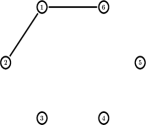
(a) $\mathcal{G}_{1}$

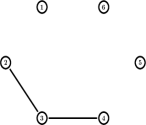
(b) $\mathcal{G}_{2}$

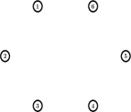
(c) $\mathcal{G}_{3}$

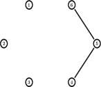
(d) $\mathcal{G}_{4}$

Figure 1: Possible interaction topologies among the agents.

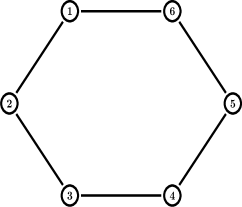
Figure 2: The union graph associated with the agents.

To solve the consensus control problem, we use the event-based protocol (2) and (5) with parameters chosen as $c=5$, $\delta=\mu=\nu=0.5$, and $G=\begin{bmatrix}0&-1\end{bmatrix}$. The states $x_{i}$, $i=1,\cdots,6$, are depicted in Fig. 3, implying that consensus is achieved. The triggering instants of all agents are presented in Fig. 4, which shows that Zeno behaviors are ruled out.

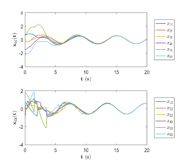
Figure 3: The state of each agent.

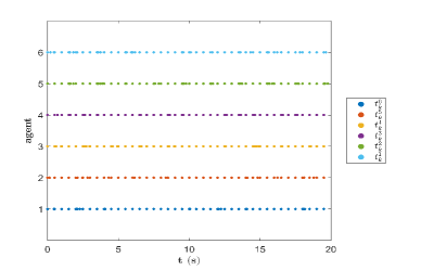
Figure 4: Triggering instants of each agent.

Example 2: The leader’s dynamics satisfies (40) with $S=\begin{bmatrix}0&1\\ -1&0\end{bmatrix}$ and the dynamics of followers are described by (39) with $A_{i}=\begin{bmatrix}-1&1\\ 0&-i\end{bmatrix}$, $B_{i}=\begin{bmatrix}0\\ i\end{bmatrix}$, $C_{i}=\begin{bmatrix}i\\ 0\end{bmatrix}$, $E_{i}=I_{2}$, $F_{i}=\begin{bmatrix}1\\ 0\end{bmatrix}$, $i=1,\cdots,4$. All agents’ initial values are randomly chosen. Suppose that possible interaction topologies shown in Fig. 5 switches as $\mathcal{\bar{G}}_{1}\rightarrow\mathcal{\bar{G}}_{2}\rightarrow\mathcal{\bar{G}}_{3}\rightarrow\mathcal{\bar{G}}_{4}\rightarrow\mathcal{\bar{G}}_{1}\rightarrow\cdots$, with the dwelling time $\tau=0.5$s. Note that node $0$ represents the leader and nodes 1-4 denote followers. It is not difficult to find that Assumptions 3-7 are satisfied.

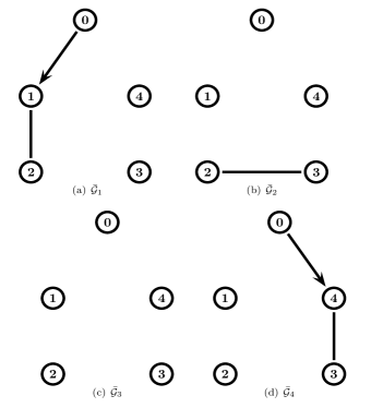
Figure 5: Possible interaction topologies.

To achieve output consensus, we utilize the event-triggered protocol (42), (47), and (54). Solving the regulation equation (41) gives $\Pi_{i}=\begin{bmatrix}1/i&1/i\\ -1&2/i\end{bmatrix}$, $U_{i}=\begin{bmatrix}-1-2/i^{2}&0\end{bmatrix}$, and $R=\begin{bmatrix}2&1\end{bmatrix}$, $i=1,\cdots,4$. Other parameters in this protocol are chosen as $c=2$, $K_{1i}=\begin{bmatrix}-1&-1\end{bmatrix}$, and $K_{2i}=\begin{bmatrix}-2-1/i-2/i^{2}&3/i\end{bmatrix}$, $i=1,\cdots,4$.

The estimate errors $w_{i}-w_{0}$, $i=1,\cdots,4$, for $t$ from $0s$ to $30s$, are depicted in Fig. 6, implying that the observers (42) can track the exogenous signal $w_{0}(t)$. Event instants of all followers are shown in Fig. 7, indicating that there exist no Zeno behaviors. The output errors $y_{i}-y_{1}$, $i=2,3,4$, are depicted in Fig. 8, implying the achievement of output consensus.

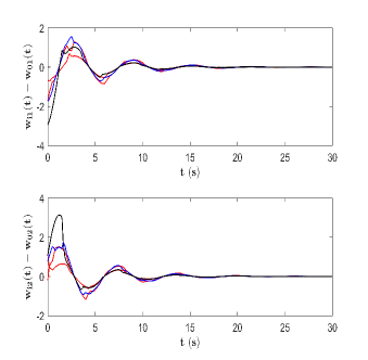
Figure 6: The estimate errors $w_{i}-w_{0}$, $i=1,\cdots,4$.

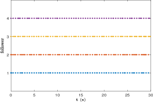
Figure 7: Triggering instants of each follower.

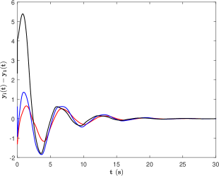
Figure 8: The output errors $y_{i}-y_{1}$, $i=2,3,4$.

V Conclusion

In this paper, distributed event-driven consensus algorithms have been proposed for homogeneous and heterogeneous linear networks with jointly connected switching topologies. These protocols can be explicitly constructed and utilized in a completely distributed manner. It is shown that the proposed protocols are able to guarantee the achievement of consensus and a strictly positive lower bound for the interval between different triggering instants. Extending these results to general directed switching graphs or fixed-time consensus [53, 54] is an interesting work in the future.

References

- [1] F. L. Lewis, H. W. Zhang, K. Hengster-Movric, and A. Das, Cooperative Control of Multi-Agent Systems: Optimal and Adaptive Design Approaches. London: Springer-Verlag, 2014.
- [2] Z. K. Li, Z. S. Duan, G. R. Chen, and L. Huang, “Consensus of multiagent systems and synchronization of complex networks: a unified viewpoint,” IEEE Trans. Circuits Syst. Regul. Pap., vol. 57, no. 1, pp. 213–224, 2010.
- [3] Z. K. Li, G. H. Wen, Z. S. Duan, and W. Ren, “Designing fully distributed consensus protocols for linear multi-agent systems with directed graphs,” IEEE Trans. Autom. Control, vol. 60, no. 4, pp. 1152–1157, 2015.
- [4] Z. K. Li and Z. S. Duan, Cooperative Control of Multi-agent Systems: A Consensus Region Approach. Boca Raton, FL: CRC Press, 2014.
- [5] Z. K. Li and J. Chen, “Robust consensus of linear feedback protocols over uncertain network graphs,” IEEE Trans. Autom. Control, vol. 62, no. 8, pp. 4251–4258, 2017.
- [6] B. A. Khashooei, D. J. Antunes, and W. P. M. H. Heemels, “Output-based event-triggered control with performance guarantees,” IEEE Trans. Autom. Control, vol. 62, no. 7, pp. 3646–3652, 2017.
- [7] Y. Q. Wu, X. Y. Meng, L. H. Xie, R. Q. Lu, H. Y. Su, and Z. G. Wu, “An input-based triggering approach to leader-following problems,” Automatica, vol. 75, pp. 221–228, 2016.
- [8] X. H. Ge and Q. L. Han, “Distributed formation control of networked multi-agent systems using a dynamic event-triggered communication mechanism,” IEEE Trans. Ind. Electron., vol. 64, no. 10, pp. 8118–8127, 2017.
- [9] L. Ding, L. Y. Wang, G. Yin, W. X. Zheng, and Q. L. Han, “Distributed energy management for smart grids with an event-triggered communication scheme,” IEEE Trans. Control Syst. Technol., vol. 27, no. 5, pp. 1950–1961, 2019.
- [10] C. Nowzari, E. Garcia, and J. Cortés, “Event-triggered communication and control of networked systems for multi-agent consensus,” Automatica, vol. 105, pp. 1–27, 2019.
- [11] C. Ramesh, H. Sandberg, L. Bao, and K. H. Johansson, “On the dual effect in state-based scheduling of networked control systems,” American Control Conf., pp. 2216–2221, 2011.
- [12] T. Henningsson, E. Johannesson, and A. Cervin, “Sporadic event-based control of first-order linear stochastic systems,” Automatica, vol. 44, no. 11, pp. 2890–2895, 2008.
- [13] K. J. Aström and B. Bernhardsson, “Comparison of periodic and event based sampling for first order stochastic systems,” Proc. IFAC World Conf., pp. 301–306, 1999.
- [14] P. Tabuada, “Event-triggered real-time scheduling of stabilizing control tasks,” IEEE Trans. Autom. Control, vol. 52, no. 9, pp. 1680–1685, 2007.
- [15] W. P. M. H. Heemels, J. H. Sandee, and P. P. J. V. D. Bosch, “Analysis of event-driven controllers for linear systems,” Int. J. Control, vol. 81, pp. 571–590, 2008.
- [16] W. P. M. H. Heemels, K. H. Johansson, and P. Tabuada, “An introduction to event-triggered and self-triggered control,” 51st IEEE Conf. on Decision and Control, pp. 3270–3285, 2012.
- [17] R. Zheng, X. L. Yi, W. L. Lu, and T. P. Chen, “Stability of analytic neural networks with event-triggered synaptic feedbacks,” IEEE Trans. Neural Netw. Learn. Syst., vol. 27, no. 2, pp. 483–494, 2016.
- [18] B. Cheng and Z. K. Li, “Fully distributed event-triggered protocols for linear multi-agent networks,” IEEE Trans. Autom. Control, vol. 64, no. 4, pp. 1655–1662, 2019.
- [19] B. Cheng and Z. K. Li, “Consensus disturbance rejection with event-triggered communications,” J. Frankl. Inst., vol. 356, no. 2, pp. 956–974, 2019.
- [20] L. Ding, Q. L. Han, X. H. Ge, and X. M. Zhang, “An overview of recent advances in event-triggered consensus of multiagent systems,” IEEE Trans. Cybern., vol. 48, no. 4, pp. 1110–1123, 2018.
- [21] X. M. Zhang, Q. L. Han, and B. L. Zhang, “An overview and deep investigation on sampled-data-based event-triggered control and filtering for networked systems,” IEEE Trans. Ind. Informat., vol. 13, no. 1, pp. 4–16, 2017.
- [22] X. M. Zhang, Q. L. Han, and X. H. Yu, “Survey on recent advances in networked control systems,” IEEE Trans. Ind. Informat., vol. 12, no. 5, pp. 1740–1752, 2016.
- [23] E. Garcia, Y. C. Cao, H. Yu, P. Antsaklis, and D. Casbeer, “Decentralised event-triggered cooperative control with limited communication,” Int. J. Control, vol. 86, no. 9, pp. 1479–1488, 2013.
- [24] X. Y. Meng and T. W. Chen, “Event based agreement protocols for multi-agent networks,” Automatica, vol. 49, no. 7, pp. 2125–2132, 2013.
- [25] D. V. Dimarogonas, E. Frazzoli, and K. H. Johansson, “Distributed event-triggered control for multi-agent systems,” IEEE Trans. Autom. Control, vol. 57, no. 5, pp. 1291–1297, 2012.
- [26] G. S. Seyboth, D. V. Dimarogonas, and K. H. Johanasson, “Event-based broadcasting for multi-agent average consensus,” Automatica, vol. 49, no. 1, pp. 245–252, 2013.
- [27] D. P. Yang, W. Ren, X. D. Liu, and W. S. Chen, “Decentralized event-triggered consensus for linear multi-agent systems under general directed graphs,” Automatica, vol. 69, pp. 242–269, 2016.
- [28] W. Zhu, Z. P. Jiang, and G. Feng, “Event-based consensus of multi-agent systems with general linear models,” Automatica, vol. 50, no. 2, pp. 552–558, 2014.
- [29] G. Guo, L. Ding, and Q. L. Han, “A distributed event-triggered transmission strategy for sampled-data consensus of multi-agent systems,” Automatica, vol. 50, no. 5, pp. 1489–1496, 2014.
- [30] H. Zhang, G. Feng, H. C. Yan, and Q. J. Chen, “Observer-based output feedback event-triggered control for consensus of multi-agent systems,” IEEE Trans. Ind. Electron., vol. 61, no. 9, pp. 4885–4894, 2014.
- [31] L. T. Xing, C. Y. Wen, F. H. Guo, Z. T. Liu, and H. Y. Su, “Event-based consensus for linear multiagent systems without continuous communication,” IEEE Trans. Cybern., vol. 47, no. 8, pp. 2132–2142, 2017.
- [32] J. Liu, Y. Yu, Q. Wang, and C. Y. Sun, “Fixed-time event-triggered consensus control for multi-agent systems with nonlinear uncertainties,” Neurocomputing, vol. 260, pp. 497–504, 2017.
- [33] X. H. Ge, Q. L. Han, and F. W. Yang, “Event-based set-membership leader-following consensus of networked multi-agent systems subject to limited communication resources and unknown-but-bounded noise,” IEEE Trans. Ind. Electron., vol. 64, no. 6, pp. 5045–5054, 2017.
- [34] W. F. Hu, L. Liu, and G. Feng, “Output consensus of heterogeneous linear multi-agent systems by distributed event-triggered/self-triggered,” IEEE Trans. Cybern., vol. 47, no. 8, pp. 1914–1924, 2017.
- [35] X. D. Liu, H. K. Liu, P. L. Lu, and S. L. Guo, “Distributed event-triggered output consensus control for heterogeneous multi-agent system with general linear dynamics,” Int. J. Syst. Sci., vol. 48, no. 11, pp. 2415–2427, 2017.
- [36] W. F. Hu and L. Liu, “Cooperative output regulation of heterogeneous linear multi-agent systems by event-triggered control,” IEEE Trans. Cybern., vol. 47, no. 1, pp. 105–116, 2017.
- [37] W. Ni and D. Z. Cheng, “Leader-following consensus of multi-agent systems under fixed and switching topologies,” Systems & Control Letters, pp. 209–217, 2010.
- [38] Y. F. Su and J. Huang, “Cooperative output regulation with application to multi-agent consensus under switching network,” IEEE Trans. Systems, Man, and Cybern. —Part B: Cybern., vol. 42, no. 3, pp. 864–875, 2012.
- [39] X. H. Ge and Q. L. Han, “Consensus of multiagent systems subject to partially accessible and overlapping markovian network topologies,” IEEE Trans. Cybern., vol. 47, no. 8, pp. 1807–1819, 2017.
- [40] B. D. Ning, Q. L. Han, Z. Y. Zuo, J. Jin, and J. C. Zheng, “Collective behaviors of mobile robots beyond the nearest neighbor rules with switching topology,” IEEE Trans. Cybern., vol. 48, no. 5, pp. 1577–1590, 2018.
- [41] A. Adaldo, F. Alderisio, D. Liuzza, G. D. Shi, D. V. Dimarogonas, M. Bernardo, and K. H. Johansson, “Event-triggered pinning control of switching networks,” IEEE Trans. Control Netw. Systems, vol. 2, no. 2, pp. 204–213, 2015.
- [42] T. H. Cheng, Z. Kan, J. R. Klotz, J. M. Shea, and W. E. Dixon, “Event-triggered control of multiagent systems for fixed and time-varying network topologies,” IEEE Trans. Autom. Control, vol. 62, no. 10, pp. 5365–5371, 2017.
- [43] Z. G. Wu, Y. Xu, R. Q. Lu, Y. Q. Wu, and T. W. Huang, “Event-triggered control for consensus of multiagent systems with fixed/switching topologies,” IEEE Trans. Syst., Man, Cybern., Syst., vol. 48, no. 10, pp. 1736–1746, 2018.
- [44] W. Y. Xu, D. W. C. Ho, L. L. Li, and J. D. Cao, “Event-triggered schemes on leader-following consensus of general linear multiagent systems under different topologies,” IEEE Trans. Cybern., vol. 47, no. 1, pp. 212–223, 2017.
- [45] R. Horn and C. Johnson, Matrix Analysis. New York, NY: Cambridge University Press, 1990.
- [46] P. A. Ioannou and J. Sun, Robust Adaptive Control. New York, NY: Prentice-Hall, 1996.
- [47] S. J. Bernau and C. B. Huijsmans, “The schwarz inequality in archimedean f-algebras,” Indag. Mathem., vol. 7, no. 2, pp. 137–148, 1996.
- [48] H. K. Khalil, Nonlinear Systems. Englewood Cliffs, NJ: Prentice-Hall, 2002.
- [49] S. Tuna, “Conditions for synchronizability in arrays of coupled linear systems,” IEEE Trans. Autom. Control, vol. 54, no. 10, pp. 2416–2420, 2009.
- [50] Y. F. Su and J. Huang, “Cooperative output regulation of linear multi-agent systems,” IEEE Trans. Autom. Control, vol. 57, no. 4, pp. 1062–1066, 2012.
- [51] J. Huang, Nonlinear Output Regulation: Theory and Applications. Philadelphia, PA, USA: SIAM, 2004.
- [52] B. Cheng and Z. K. Li, “Event-triggered consensus of multi-agent systems with jointly connected switching topologies,” 2018 IEEE Conf. on Control Techn. and Applic., pp. 1072–1077, 2018.
- [53] B. D. Ning, Q. L. Han, and Z. Y. Zuo, “Distributed optimization for multiagent systems: an edge-based fixed-time consensus approach,” IEEE Trans. Cybern., vol. 49, no. 1, pp. 122–132, 2019.
- [54] Z. Y. Zuo, Q. L. Han, B. D. Ning, X. H. Ge, and X. M. Zhang, “An overview of recent advances in fixed-time cooperative control of multiagent systems,” IEEE Trans. Ind. Informat., vol. 14, no. 6, pp. 2322–2334, 2018.