The twist-cofinite topology on the mapping class group of a surface

Abstract.

A topology is defined on the mapping class group $\mathrm{Mod}(\Sigma)$ of a compact connected orientable surface $\Sigma$. It is shown that a notion of “genericity” on subsets of $\mathrm{Mod}(\Sigma)$ arises from this definition. Many plausible results follow from this notion easily; for example, the set of pseudo-Anosov maps is shown to be generic, and can be assumed to have arbitrary large stretch factor, generically. Let $M$ be a 3-manifold obtained from a Heegaard splitting of fixed genus $g$ and generic gluing map. It is shown that for such manifolds, generically $b_{1}(M)=0,$ $M$ is hyperbolic and $M$ has Heegaard genus exactly $g.$

1. Introduction

Let $\Sigma$ be a closed, compact, connected orientable surface of genus $g\geq 2.$ The mapping class group of $S$ is the group $\mathrm{Mod}(\Sigma)=\pi_{0}(\mathrm{Diff}^{+}(\Sigma))$ of isotopy classes of positively oriented diffeomorphisms of $S.$ For any property $\mathcal{P}(f)$ depending on a mapping class $f\in\mathrm{Mod}(\Sigma),$ one may ask whether the property $\mathcal{P}(f)$ is true for a generic element of $\mathrm{Mod}(\Sigma).$

Such questions have been investigated by various authors, for example, [3] [15] [14] [8]. Although there are many possible notions of genericity of a mapping class group element, in most of the above works, genericity is defined using the following measure theoretic definition: Choose a finite generating set $S$ of $\mathrm{Mod}(\Sigma),$ and let $W_{n}$ be a random variable in $\mathrm{Mod}(\Sigma)$ which is obtained by an $n$-step random walk in the Cayley graph of $\mathrm{Mod}(\Sigma),$ starting at the identity. Then the property $\mathcal{P}$ is said to be generic if

$$\mathbb{P}_{n\rightarrow\infty}(\mathcal{P}(W_{n})\ \textrm{is true})\rightarrow 1.$$

In the paper [15], several versions of the notion of random elements of $\mathrm{Mod}(\Sigma)$ are developed, but these notions of genericity stay probabilistic in nature.

For subsets of ${\mathbb{R}},$ there are two alternative notions of being generic:

• A measure theoretic one, stating that a subset $S\subset{\mathbb{R}}$ is generic (in the sense of Lebesgue) if ${\mathbb{R}}\setminus S$ has Lebesgue measure $0.$

• A topological one, stating that $S$ is generic (in the sense of Baire) if $S$ contains a countable intersection of open dense subsets of ${\mathbb{R}}.$

The aim of this paper is to develop a topological notion of genericity of a subset of the mapping class group. In order to achieve this goal, in [2], a topology on $\mathrm{Mod}(\Sigma)$ called the twist-cofinite topology was defined. For $\gamma$ a non-trivial simple closed curve on $\Sigma,$ let $D_{\gamma}$ be the Dehn-twist around $\gamma.$

Theorem 1.

Let

$$\mathcal{O}=\{U\subset\mathrm{Mod}(\Sigma)\ |\ \forall f\in U,\forall\gamma,f\circ D_{\gamma}^{n}\in U\ \textrm{for all }n\in{\mathbb{Z}}\ \textrm{except at most finitely many n}\}.$$

Then $\mathcal{O}$ is a topology on $\mathrm{Mod}(\Sigma),$ and $\mathrm{Mod}(\Sigma)$ is a connected topological group for this topology.

A fundamental property of this topology, similar for example to the Zariski topology, is that open sets are quite large. Specifically, a subset $S$ of $\mathrm{Mod}(\Sigma)$ will be called thick if $S$ has non-empty interior. The next proposition suggests that thickness of a subset is a good notion of genericity:

Proposition 2.

In the topology $\mathcal{O},$

• The intersection $U_{1}\cap U_{2}$ of two non-empty open sets $U_{1}$ and $U_{2}$ is non-empty.

• Any thick subset is dense.

• The intersection of any finite collection $S_{1},\ldots,S_{k}$ of thick subsets is thick.

With this notion of genericity, generic properties of subsets of $\mathrm{Mod}(\Sigma)$ will be studied. For example,

Theorem 3.

The following subsets of $\mathrm{Mod}(\Sigma)$ are non-empty and open (i.e. thick):

• The set of pseudo-Anosov maps $f\in\mathrm{Mod}(\Sigma).$

• The sets $\{f\in\mathrm{Mod}(\Sigma)\ \textrm{pseudo-Anosov}\ |\ \mathrm{Vol}(M_{f})>C\},$ where $M_{f}$ is the mapping torus of $f$ and $C>0.$

• The sets $\{f\in\mathrm{Mod}(\Sigma)\ \textrm{pseudo-Anosov}\ |\ \lambda(f)>C\},$ where $\lambda(f)$ is the stretch factor of $f$ and $C>0.$

• The set of pseudo-Anosovs that do not leave any integer homology class of curves on $\Sigma$ invariant.

In [3] Dunfield and Thurston used the measure theoretic notion of genericity in $\mathrm{Mod}(\Sigma)$ and Heegaard splittings to study the genericity of various properties of $3$-manifolds. The same notion of random $3$-manifolds was studied in subsequent papers [15] [14] and [8] by various authors.

Similar can be done with the notion of thickness/genericity defined above.

Let $H_{A}$ and $H_{B}$ be a pair of handlebodies, with $\partial H_{A}=\partial H_{B}=\Sigma$. For $f\in\mathrm{Mod}(\Sigma),$ let $N_{f}$ be the $3$-manifold:

$$N_{f}=H_{A}\underset{f}{\bigcup}H_{B}$$

where $f$ is called the gluing map of a Heegaard splitting of $N_{f}.$ The properties of $3$-manifold invariants of $N_{f}$ for a generic $f$ can be studied. Some of the simplest such invariants are first Betti numbers.

Theorem 4.

The following are all thick:

1. The set $\{f\in\mathrm{Mod}(\Sigma)\ |\ b_{1}(N_{f},\mathbb{Z})=0\}$

2. The set $\{f\in\mathrm{Mod}(\Sigma)\ |\ |H_{1}(N_{f},{\mathbb{Z}})|\geqslant k\}$ for any integer $k\geqslant 0$

Here $b_{1}(N_{f},\mathbb{Z})$ is the first Betti number of $N_{f}$, and $|H_{1}(N_{f},{\mathbb{Z}})|$ is the number of elements in the group $H_{1}(N_{f},{\mathbb{Z}})$. Suppose $p$ is prime and $0\leqslant i\leqslant g$. Similar arguments show that the set $\{f\in\mathrm{Mod}(\Sigma)\ |\ b_{1}(N_{f},\mathbb{F}_{p})=i\}$ is dense but not thick.

The following will also be proven, using somewhat different techniques:

Theorem 5.

The set $\{f\in\mathrm{Mod}(\Sigma)\ |\ g(N_{f})=g(\Sigma)\}$ is thick, where $g(N_{f})$ is the Heegaard genus of $N_{f}$.

A natural question to ask is whether, with this notion of genericity, a generic Heegaard splitting gives an irreducible manifold and whether it gives a hyperbolic manifold. Note that, due to the Geometrization theorem, being hyperbolic is equivalent to being irreducible and atoroidal. A more general guestion is therefore, whether $N_{f}$ admits an incompressible surface of genus $\leqslant g$.

Theorem 6.

For any $g\geqslant 0,$ the set

$$\{f\in\mathrm{Mod}(\Sigma)\ |\ N_{f}\ \textrm{has no incompressible surface of genus }\leqslant g\}$$

is thick.

This theorem will be reduced to studying a property of Hempel’s distance in Harvey’s complex of curves. Hempel’s distance also gives a lower bound on the genus of an incompressible surface. Theorem 6 will be shown to follow from Theorem 7 below:

Theorem 7.

For any $d\geqslant 0,$ the set

$$\{f\in\mathrm{Mod}(\Sigma)\ |\ \textrm{the Heegaard splitting induced by }f\ \textrm{has distance}\geqslant d\}$$

is an open dense set.

While most of the results in this paper follow almost immediately from the definitions or from classical results, the proof of a lemma needed for these last two theorems is quite long and technical.

On page 3 of [14], a list of properties of elements of subgroups of mapping class groups represented by random long words in a symmetric generating set is given. On page 4 of the same paper, a list of properties of random Heegaard splittings according to the Dunfield-Thurston model is given. The properties investigated for genericity in this paper are based on these two lists. Results in this paper should be compared with theorems in [14] and the extensive list of references given therein. Given the amount of literature available on the subject, the author apologises that no attempt is made here to do justice to related results in different frameworks.

As a final comment, the notion of genericity developed here has advantages and disadvantages. The measure theoretic definition of genericity a priori depends on the choice of a finite generating set of $\mathrm{Mod}(\Sigma).$ Genericity of a property in that setting is often shown for one generating set only, such as the set of Humphries generators. It follows that the topological notion of genericity is more canonical, as it does not depend on any choice. In addition, it is suited to formulating problems about subgroups of mapping class groups. These properties can be understood in terms of subset topologies. An example of such a problem is the well known Ivanov conjecture, [5]. When $\Sigma$ has genus at least 3, the Ivanov conjecture predicts that any finite index subgroup $\Gamma$ of $\mathrm{Mod}(\Sigma)$ satisfies $H_{1}(\Gamma,\mathbb{R})=0$.

On the other hand, the measure theoretic version is better suited to asking questions about the asymptotic growth of invariants (stretch factor, volume of the mapping torus, etc…) of “generic mapping classes”. It is possible to simply study the average value of the invariant of the $n$-step random walk $W_{n}$.

The paper is organised as follows: In Section 2, topologies $\mathcal{O}_{G,S}$ on groups $G$ equiped with a generating set $S$ are defined. The general properties of those topologies are studied and it is shown that the twist-cofinite topology is obtained as an example of such a topology, taking $G=\mathrm{Mod}(\Sigma)$ and $S$ to be the set of all Dehn-twists. Theorem 1 and Proposition 2 are corollaries of this more general theory. In Section 3, generic properties of elements of $\mathrm{Mod}(\Sigma)$ are discussed, and Theorem 3 is proven. Sections 4 and 5 deal with properties of $3$-manifolds obtained from generic Heegaard splittings. The proof of Theorem 7 requires concepts such as subsurface projections, due to Masur and Minsky, and properties of handlebody sets, due to Masur and Schleimer. This background material is given in Subsections 5.2 and 5.3, as well as a crucial property of bounded and unbounded diameter subsurface projections of handlebody sets. The remainder of Section 5 deals mainly with showing the existence of certain large subsurface projections needed to obtain distance bounds in the proof of Theorem 7.

Acknowledgments

As noted above, the definition of the twist cofinite topology comes from Renaud Detcherry, and the first two subsections of this paper were also taken from [2], with the author’s permission. The proof of Lemma 18 benefitted from discussions with Saul Schleimer.

2. A topology on groups with generating sets

Let $G$ be a group and $S$ be a generating set for $G.$ For $g\in G,$ let $L_{g}$ be the left multiplication:

$$\begin{array}[]{rccl}L_{g}:&G&\longrightarrow&G\\ &h&\longrightarrow&gh\end{array}$$

and $R_{g}$ be the right multiplication:

$$\begin{array}[]{rccl}R_{g}:&G&\longrightarrow&G\\ &h&\longrightarrow&hg.\end{array}$$

Let also $s:G\rightarrow G$ be the map such that $s(g)=g^{-1}.$ Two topologies on $G$ are defined:

Definition 8.

Let

$$\mathcal{O}_{G,S}^{l}=\{U\subset G\ |\ \forall g\in U,\forall x\in S,\text{ For all except at most finitely many }n\in{\mathbb{Z}}\ ,\ gx^{n}\in U\}$$

and

$$\mathcal{O}_{G,S}^{r}=\{U\subset G\ |\ \forall g\in U,\forall x\in S,\text{For all exacept at most finitely many }n\in{\mathbb{Z}}\ \ x^{n}g\in U\}.$$

Let $\mathcal{O}_{G,S}=\mathcal{O}_{G,S}^{r}\cap\mathcal{O}_{G,S}^{l}.$

Theorem 9.

The sets $\mathcal{O}_{G,S}^{l}$ (resp. $\mathcal{O}_{G,S}^{r}$) determine a topology on $G$ for which the operator $L_{g}$ (resp. $R_{g}$) is continuous for any $g\in G$. In addition, $G$ is a topological group for the topology $\mathcal{O}_{G,S}$, and $G$ is connected for all three topologies.

The left (resp. right) cyclically cofinite topology on $G$ relative to the generating set $S$ refers to the set of open sets $\mathcal{O}_{G,S}^{l}$ (resp. $\mathcal{O}_{G,S}^{r}$). The set of open sets $\mathcal{O}_{G,S}$ determines the cyclically cofinite topology on $G$ relative to $S.$

The motivation for those names is that the intersection of an open set in $\mathcal{O}_{G,S}^{l}$ with a left coset of a cyclic subgroup of $G$ generated by an element of $S$ is either empty or cofinite.

Proof.

It will be shown that $\mathcal{O}_{G,S}^{l}$ is a topology; the case of $\mathcal{O}_{G,S}$ is analogous.

The empty set and $G$ are both in $\mathcal{O}_{G,S}^{l}.$ Suppose $U_{1}$, $U_{2}\in\mathcal{O}_{G,S}^{l}$, $g\in U_{1}\cap U_{2},$ and let $x$ be in $S.$ Then $gx^{n}\in U_{1}$ except for at most finitely many $n\in{\mathbb{Z}},$ and $gx^{n}\in U_{2}$ except for at most finitely many $n\in{\mathbb{Z}}.$ It follows that $gx^{n}\in U_{1}\cap U_{2}$ except for at most finitely many $n\in{\mathbb{Z}}.$ Therefore $U_{1}\cap U_{2}$ is in $\mathcal{O}_{G,S}^{l}.$

Now it will be shown that an arbitrary union of open sets is open. Let $(U_{i})_{i\in I}$ be a family of elements of $\mathcal{O}_{G,S}^{l},$ and $U=\underset{i\in I}{\bigcup}U_{i}.$ Let $g\in U$ and $x\in S,$ then $g\in U_{i}$ for some $i,$ and $gx^{n}\in U_{i}$ for all $n\in{\mathbb{Z}}$ except at most finitely many. In particular $gx^{n}\in U$ for all but finitely many $n.$ Therefore $\mathcal{O}_{G,S}^{l}$ is a topology.

It will now be shown that for any $g\in G,$ the operator $L_{g}$ is continuous (in the topology $\mathcal{O}_{G,S}^{l}$), or equivalently, for any open set $U,$ that $g^{-1}U$ is also open. Let $g^{-1}h\in g^{-1}U.$ As $U$ is open, for any $x\in S,$ all but finitely many $hx^{n}$ are in $U$ and all but finitely many $g^{-1}hx^{n}$ are in $g^{-1}U.$ Therefore $g^{-1}U$ is open.

Similarly, $R_{g}$ is continuous on $G$ for the topology $\mathcal{O}_{G,S}^{r}.$

To show connectivity, assume that $U$ is a nonempty open and closed subset of $G$ for the topology $\mathcal{O}_{G,S}^{l}.$ Let $g\in U$ and $x\in S,$ then since $U$ is open, $gx^{n}\in U$ for all but at most finitely many $n$. In fact, $gx^{n}\in U$ for all $n\in{\mathbb{Z}}$. To see why, note that if $gx^{i}\in G\setminus U$ for some $i,$ then as $G\setminus U$ is also open, $gx^{n}\in G\setminus U$ for all but finitely many $n\in{\mathbb{Z}},$ hence one can find an integer $n$ such that $gx^{n}\in U\cap(G\setminus U)=\emptyset,$ giving a contradiction. It follows that $G$ is connected for the topology $\mathcal{O}_{G,S}^{l},$ and similarly also for the topology $\mathcal{O}_{G,S}^{r}.$

For the intersection topology $\mathcal{O}_{G,S},$ $G$ will also be connected and for any $g\in G,$ both $L_{g}$ and $R_{g}$ are continuous. To show that $G$ with the topology $\mathcal{O}_{G,S}$ is a topological group, it remains to show that the inversion map $s:G\rightarrow G$ is continuous, or equivalently, that for any open $U\in\mathcal{O}_{G,S},$ $U^{-1}\in\mathcal{O}_{G,S}.$

Let $U\in\mathcal{O}_{G,S},$ $g^{-1}\in U^{-1}$ and $x\in S.$ Then $gx^{n}\in U$ and $x^{n}g\in U$ for all but finitely many $n\in{\mathbb{Z}}.$ It follows that $x^{-n}g^{-1}\in U^{-1}$ and $g^{-1}x^{-n}\in U^{-1}$ for all but finitely many $n\in{\mathbb{Z}},$ hence $U^{-1}\in\mathcal{O}_{G,S}.$ Therefore $s$ is continuous and $G$ is a topological group, for the topology $\mathcal{O}_{G,S}.$ ∎

Having constructed those topologies, it remains to be seen that they are interesting topologies. At the very least, one would want them to be non-trivial. It will be shown in Section 3 and 4 that in the example in which $G=\mathrm{Mod}(\Sigma)$ for some compact connected oriented surface $\Sigma$ with $S$ being the set of all Dehn-twists, there are many interesting open sets. However, at this level of generality, the non-triviality of the topology $\mathcal{O}_{G,S}$ depends on the properties of the generating set $S,$ in particular the orders of elements in $S:$

Proposition 10.

Let $G$ be a group and $S$ a generating set for $G.$

• If the generating set consists only of elements of infinite order, then $\mathcal{O}_{G,S}^{l},\mathcal{O}_{G,S}^{r}$ and $\mathcal{O}_{G,S}$ are all finer than the cofinite topology on $G$.

• In addition, if for any $x\neq y\in S,$ then $\langle x\rangle\cap\langle y\rangle=\{1\},$ then $\mathcal{O}_{G,S}^{l},\mathcal{O}_{G,S}^{r}$ and $\mathcal{O}_{G,S}$ are strictly finer.

• If, on the other hand, the generating set consists only of elements of finite order, $\mathcal{O}_{G,S}^{l},\mathcal{O}_{G,S}^{r},\mathcal{O}_{G,S}$ are all the trivial topology on $G.$

Proof.

Both claims will be proven only for $\mathcal{O}_{G,S}^{l}$; the case of $\mathcal{O}_{G,S}^{r}$ being similar, and the case of $\mathcal{O}_{G,S}$ being a consequence of the first two cases by taking the intersection.

Assume first that $S$ contains only elements of infinite order. It is necessary to show that for any finite subset $V\subset G,$ the set $G\setminus V$ is open. Let $h\in G\setminus V$ and $x\in S.$ As $x$ has infinite order in $G,$ the elements $hx^{n}$ are all different, therefore all but at most finitely many are in $G\setminus V.$ Hence $G\setminus V$ is open, and $\mathcal{O}_{G,S}^{l}$ is finer than the cofinite topology on $G.$

Now assume also that $\langle x\rangle\cap\langle y\rangle=\{1\}$ for any two distinct elements of $S.$ It will now be shown that for any generator $x\in S,$ then $G\setminus\langle x\rangle\in\mathcal{O}_{G,S}^{l}.$

Let $g\in G\setminus\langle x\rangle.$ Then $gx^{n}\notin\langle x\rangle$ for any $n\in{\mathbb{Z}}.$ Let $y\in S$ be another generator. Then $gy^{n}\in\langle x\rangle$ for at most 1 integer $n\in{\mathbb{Z}}.$ If $gy^{i},gy^{j}\in\langle x\rangle$ for $i\neq j,$ then $y^{j-i}\in\langle x\rangle\cap\langle y\rangle.$ But $y^{j-i}\neq 1$ as $y$ has infinite order which contradicts the fact that $\langle x\rangle\cap\langle y\rangle=\{1\}.$

Finally, assume that $S$ consists only of finite order elements. Let $U\in\mathcal{O}_{G,S}^{l}$ be a non-empty open set, and let $g\in U$ and $x\in S.$ Assume that $x^{d}=1.$ Then all but at most finitely many elements $gx^{1+kd}$ where $k\in{\mathbb{Z}}$ are in $U.$ But $gx^{1+kd}=gx$ so $gx\in U.$ Similarly, one shows that $gx^{-1}\in U.$

Therefore $U$ is closed by multiplication on the right by any element in $S$ or any inverse of an element in $S.$ The set $S$ being a generating set of $G,$ this means that $U=G.$ Then $\mathcal{O}_{G,S}^{l}$ is the trivial topology in this case. ∎

The cyclically-cofinite topologies relative to a generating set are compatible with morphisms of groups, as the following proposition shows:

Proposition 11.

Let $\phi:G\rightarrow H$ be a surjective morphism of groups and $S$ be a generating set of $G$. Then $\phi(S)$ is a generating set for $H,$ and for the topologies $\mathcal{O}_{G,S}^{l}$ and $\mathcal{O}_{H,\phi(S)}^{l}$ (or with $\mathcal{O}_{G,S}^{r}$ and $\mathcal{O}_{H,\phi(S)}^{r}$, or $\mathcal{O}_{G,S}$ and $\mathcal{O}_{H,\phi(S)}$) the map $\phi$ is continuous.

Proof.

The set $\phi(S)$ is a generating set for $H$ as $\phi$ is a surjective morphism. Once again the statement will be proven for the left cyclically-cofinite topologies only.

Let $U\in\mathcal{O}_{H,\phi(S)}^{l},$ and let $g\in\phi^{-1}(U).$ For any $x\in S,$ then $\phi(gx^{n})=\phi(g)\phi(x)^{n}\in U$ for all but finitely many $n\in{\mathbb{Z}},$ as $U$ is open. Therefore $\phi^{-1}(U)\in\mathcal{O}_{G,S}^{l},$ and $\phi$ is continuous. ∎

When the generating set $S$ is closed under conjugation by an arbitrary element of $G,$ the above topologies are better behaved:

Proposition 12.

Assume that $S$ is a generating set for a group $G$ that is closed under conjugation by any element of $G.$ Then the topologies $\mathcal{O}_{G,S}^{r},\mathcal{O}_{G,S}^{l}$ and $\mathcal{O}_{G,S}$ all coincide.

Also, the intersection of any two non-empty open subsets of $G$ is a non-empty open subset of $G$.

Proof.

Let $U\in\mathcal{O}_{G,S}^{l}$ and let $g\in U.$ Then for any $x\in S,$ the element $g^{-1}xg\in S$ as $S$ is closed under conjugation. Therefore $x^{n}g=g(g^{-1}xg)^{n}\in U$ for all but at most finitely many $n\in{\mathbb{Z}}.$ This shows that $U\in\mathcal{O}_{G,S}^{r}$ and $\mathcal{O}_{G,S}^{l}\subset\mathcal{O}_{G,S}^{r}.$

Similarly, $\mathcal{O}_{G,S}^{r}\subset\mathcal{O}_{G,S}^{l}$ and hence $\mathcal{O}_{G,S}^{l}=\mathcal{O}_{G,S}^{r}=\mathcal{O}_{G,S}.$

Now let $U_{1}$ and $U_{2}$ be two non-empty open sets of $G.$ For $g\in U_{1}$ and $h\in U_{2},$ as $S$ is a generating set, one can write:

$$h=gx_{1}^{i_{1}}x_{2}^{i_{2}}\ldots x_{k}^{i_{k}}$$

for some $k\geqslant 0,$ some $x_{j}\in S$ and $i_{j}\in{\mathbb{Z}}.$ It will be shown that one can find $g\in U_{1}$ and $h\in U_{2}$ so that one can assume $k=0,$ which would mean that $g=h\in U_{1}\cap U_{2}.$

Let $g\in U_{1}$ and $h\in U_{2}.$ As $U_{2}$ is open, $hx_{k}^{n}\in U_{2}$ for all but finitely many $n\in{\mathbb{Z}}.$ Also $gx_{k}^{m}\in U_{1}$ for all but finitely many $m\in{\mathbb{Z}}.$ In particular, one can choose $n$ and $m$ such that $hx_{k}^{n}\in U_{2},$ $gx_{k}^{m}\in U_{1}$ and $m=i_{k}+n.$ Then

$$hx_{k}^{n}=(gx_{k}^{m})x_{k}^{-m}x_{1}^{i_{1}}\ldots x_{k}^{i_{k}+n}=(gx_{k}^{m})x_{k}^{-m}x_{1}^{i_{1}}\ldots x_{k}^{m}=(gx_{k}^{m})y_{1}^{i_{1}}\ldots y_{k-1}^{i_{k-1}}$$

where $y_{j}=x_{k}^{-m}x_{j}x_{k}^{m}\in S$ as $S$ is closed under conjugation. Therefore it is possible to inductively decrease $k$ by $1$ until $k=0$ is obtained, showing that $U_{1}\cap U_{2}\neq\emptyset.$ ∎

Proposition 12 implies that if $S$ is a generating set with the property of being closed under conjugation by $G,$ then any non-empty open set in $\mathcal{O}_{G,S}$ is dense.

As in the introduction, call a subset $V\subset G$ thick if it has non-empty interior, and thin if its complement is thick. Any thick set is dense as its interior is dense, and any intersection of two thick sets is thick as the intersection of their interiors is a non-empty open set.

It will sometimes be necessary to consider sets which are dense but not thick. An example will be given in Theorem 4.

Lemma 13.

Let $G$ be a group and $S$ be a generating set for $G$ that is closed under conjugation. Let $V$ be a non-empty subset of $G$ such that for any $g\in V,$ and any $x\in S,$ infinitely many $gx^{n}$ are in $V.$ Then $V$ is dense in $G$ for the topology $\mathcal{O}_{G,S}$.

Proof.

As in the proof of Proposition 12, consider $g\in U$, where $U$ is a non-empty open set and $h\in V$, where $V$ satisfies the hypothesis of the proposition. Then

$$h=gx_{1}^{i_{1}}x_{2}^{i_{2}}\ldots x_{k}^{i_{k}}$$

for some $k\geqslant 0$ and $x_{j}\in S.$ Therefore the set $T=\{m\in{\mathbb{Z}}\ |hx_{k}^{m}\in V\}$ is infinite.

Moreover $gx_{k}^{n}\in U$ for all but finitely many $n\in{\mathbb{Z}},$ and hence there is some $n$ in $\{m-i_{k}\ |m\in T\}$ such that $gx_{k}^{n}\in U.$ As in the previous proof it follows that one could find another pair $g^{\prime}\in U,h^{\prime}\in V$ with $h^{\prime}=g^{\prime}y_{1}^{j_{1}}\ldots y_{k-1}^{j_{k-1}}$ with all $y_{l}$’s in $S.$ By induction, it follows that $U\cap V\neq\emptyset.$ Hence $V$ has non-empty intersection with any open set, i.e. $V$ is dense. ∎

The twist-cofinite topology defined in Theorem 1 is an example of such a topology, where $G=\mathrm{Mod}(\Sigma)$ for some compact connected oriented surface $\Sigma,$ and $S$ is the set of all Dehn-twists. The set of all Dehn-twists generates $\mathrm{Mod}(\Sigma)$ and is closed under conjugation; if $f\in\mathrm{Mod}(\Sigma)$ and $D_{\gamma}$ is a Dehn-twist around a curve $\gamma$ on $\Sigma,$ then $f\circ D_{\gamma}\circ f^{-1}=D_{f(\gamma)}.$ Therefore Theorem 1 and Proposition 2 are consequences of the more general Definition 8 and Proposition 12 above.

3. Generic properties of pseudo-Anosovs

In this section, Theorem 3 will be obtained as a corollary of classical results.

Theorem (Theorem 3 of the introduction).

The following subsets of $\mathrm{Mod}(\Sigma)$ are non-empty and open, and hence thick:

1. The set of pseudo-Anosov maps $f\in\mathrm{Mod}(\Sigma).$

2. The sets $\{f\in\mathrm{Mod}(\Sigma)\ \textrm{pseudo-Anosov}\ |\ \mathrm{Vol}(M_{f})>C\},$ where $M_{f}$ is the mapping torus of $f$ and $C>0.$

3. The sets $\{f\in\mathrm{Mod}(\Sigma)\ \textrm{pseudo-Anosov}\ |\ \lambda(f)>C\},$ where $\lambda(f)$ is the stretch factor of $f$ and $C>0.$

4. The set of pseudo-Anosovs that do not leave any integer homology class of curves on $\Sigma$ invariant.

Proof.

The first part of the theorem follows directly from the following

Theorem 14 (Theorem A part $i$ of [7]).

Let $f:\Sigma\rightarrow\Sigma$ be a pseudo-Anosov map, and $c$ a simple curve on $\Sigma$. Then for all but at most finitely many $n$, the composition $D_{c}f$ is also pseudo-Anosov

To prove the second part of the Theorem, note that $N_{fD_{c}^{n}}$ is obtained from $N_{f}$ by a Dehn surgery. The behaviour of volume under Dehn surgeries has been studied in [13], where it follows from Theorem 1A that for sufficiently large $|n|$

$$\mathrm{Vol}(M_{f})<\mathrm{Vol}(M_{fD_{c}^{n}})$$

Similarly for $\mathrm{Vol}(M_{D_{c}^{n}f})$.

The third part of the theorem also follows directly from a Theorem of [7]. It is a consequence of Theorem C of [7] that there are positive constants $K$, $L_{1}$ and $L_{2}$ such that

$$|n|L_{1}-K\leq\lambda(D_{c}^{n}f)\leq L_{2}|n|+K$$

Denote by $[c]$ the integer homology class in $H_{1}(\Sigma,\mathbb{Z})$ with representative $c$. If $[c]=0$, the action of the mapping class $f$ on homology is identical to that of $fD_{c}^{n}$ or $D_{c}^{n}f$. If $c$ is a nonseparating curve, choose a set of curves containing $c$ that determine a symplectic basis for $H_{1}(\Sigma,\mathbb{Z})$, and denote by $d$ the unique curve in the set intersecting $c$. Since the action of the mapping class group on $\pi_{1}(\Sigma)$ defines an action on $H_{1}(\Sigma,\mathbb{Z})$, the action of a mapping class on $H_{1}(\Sigma,\mathbb{Z})$ is determined by its action on the curves making up the chosen basis. It follows immediately that there is at most one value of $n$ for which $fD_{c}^{n}$ acts trivially on homology. Replacing the set of curves making up the basis by their images under $f^{-1}$, the same argument shows the same is true for $D_{c}^{n}f$. Therefore, the set of pseudo-Anosovs that do not leave any integer homology class of curves on $\Sigma$ invariant is open. This set is known to be non-empty, so the theorem follows. ∎

Since Dehn twists are not of finite order in the mapping class group, it follows immediately from Proposition 10 that the subgroups of the mapping class group in Theorem 3 are also generic in finite index subgroups of mapping class groups. In [9], it was shown that there is a sense in which pseudo-Anosovs are generic in every finitely generated subgroup of $\mathrm{Mod}(\Sigma)$ containing a pseudo-Anosove element. Apart from this, little seems to be known about subset topologies.

4. Heegaard splittings of $3$-manifolds with generic gluing maps

In this section, the homology of 3-manifolds described as Heegaard splittings with generic gluing maps will be studied. A reference for any facts about Heegaards splitting used here is [6].

The homology of a 3-manifold can be computed from a Heegaard splitting, using Mayer-Vietoris. If $g$ is the genus of $\Sigma$, then

$$H_{2}(N_{f};\mathbb{Z})\rightarrow H_{1}(\Sigma,\mathbb{Z})=\mathbb{Z}^{2g}\rightarrow H_{1}(H_{A};\mathbb{Z})\bigoplus H_{1}(H_{B};\mathbb{Z})=\mathbb{Z}^{g}\bigoplus\mathbb{Z}^{g}\rightarrow H_{1}(N_{f};\mathbb{Z})$$

To compute $H_{2}(N_{f};\mathbb{Z})$ and $H_{1}(N_{f};\mathbb{Z})$ it is therefore necessary to calculate the $2g\times 2g$ matrix $A(f)$ describing the map $H_{1}(\Sigma;\mathbb{Z})\rightarrow H_{1}(H_{A};\mathbb{Z})\bigoplus H_{1}(H_{B};\mathbb{Z})$.

Let $\{x_{1},\ldots,x_{2g}\}$ be a generating set for $\pi_{1}(\Sigma)$. For $H_{A}$ let $a_{1},\ldots,a_{g}$ be a set of curves on $\Sigma$ that bound a set of disks in $H_{A}$. Suppose also that when $H_{A}$ is cut along these disks, a ball is obtained. The curves $\{b_{1},\ldots,b_{g}\}$ are defined similarly for $H_{B}$. Each curve $a_{i}$ or $b_{i}$, $i=1,\ldots,g$ is described by a word in the generators $\{x_{1},\ldots,x_{2g}\}$. The first row of $A(f)$ is the vector representing $[a_{1}]$ in the basis $\{[x_{1}],\ldots,[x_{2g}]\}$, the second row is the vector representing $[a_{2}]$, then $[a_{3}],\ldots,[a_{g}],[b_{1}],\ldots,[b_{g}]$.

Lemma 15 (Lemma 3.31 of [6]).

$H_{1}(N_{f};\mathbb{Z})$ is finite iff the determinant of $A$ is nonzero. In addition, if $H_{1}(N_{f};\mathbb{Z})$ is finite then the order of $H_{1}(N_{f};\mathbb{Z})$ is equal to the absolute value of the determinant of $A$.

Theorem 16 (Theorem 4 of the introduction).

Suppose $b_{1}(N_{f},\mathbb{Z})$ is the first Betti number of $N_{f}$, and $|H_{1}(N_{f},{\mathbb{Z}})|$ is the number of elements in the group $H_{1}(N_{f},{\mathbb{Z}})$. Then

1. The set $\{f\in\mathrm{Mod}(\Sigma)\ |\ b_{1}(N_{f},\mathbb{Z})=0\}$ is a thick set

2. The set $\{f\in\mathrm{Mod}(\Sigma)\ |\ |H_{1}(N_{f},{\mathbb{Z}})|\geqslant k\}$ for any integer $k\geqslant 0$ is a thick set

3. If $p$ is prime and $0\leqslant i\leqslant g$, the set $\{f\in\mathrm{Mod}(\Sigma)\ |\ b_{1}(N_{f},\mathbb{F}_{p})=i\}$ is dense but not thick.

Proof.

By Lemma 15, proving the first part of the theorem is the same as showing that the set $\{f\in\mathrm{Mod}(\Sigma)\ |\ detA(f)\neq 0\}$ is thick. Since this set is clearly nonempty, it suffices to show that the set is open. Consider the map from $A(f)$ to $A(fD_{c}^{n})$. This map fixes the last $g$ rows, and adds the vector $n\hat{i}(a_{i},c)[c]$ to row $i$, for $1\leq i\leq g$. Here $\hat{i}$ denotes algebraic intersection number, and $[c]$ is assumed to be a vector representing the homology class with representative $c$ in the basis $\{[x_{1}],\ldots,[x_{2g}]\}$.

Since the determinant of $A$ is nonzero, $[a_{1}],\ldots,[a_{g}]$ and $[b_{1}],\ldots,[b_{g}]$ can be chosen such that $[c]$ is in the span of $[a_{g}]$ and $[b_{1}]$. It follows that the determinant of $A(fD_{c}^{n})$ can only be zero if the projection of $n\hat{i}(a_{i},c)[c]$ onto the unit vector parallel to $[a_{g}]$ is given by $-[a_{g}]$. This can happen for at most one value of $n$.

Similarly, consider the map from $A(f)$ to $A(D_{c}^{n}f)$. This map fixes the first $g$ rows, and adds the vector $n\hat{i}(b_{i},c)[c]$ to row $i+g$, for $1\leq i\leq g$. The same argument as before shows that the determinant of $A(D_{c}^{n}f)$ can only be zero for finitely many $n$. This proves the first part of the theorem.

From the expressions for $A(fD_{c}^{n})$ and $A(D_{c}^{n}f)$ just given, it follows that for $n^{*}$ sufficiently large, $n>n^{*}$ implies that $|detA(fD_{c}^{n})|\geq|det(A)|$ and $|detA(D_{c}^{n}f)|\geq|det(A)|$. The second part of the theorem is then a consequence of Lemma 15.

To prove the last part of the theorem, note that $b_{1}(N_{f},\mathbb{F}_{p})$ is equal to the dimension of the kernel of $A_{f}\mod p$. Similarly for $b_{1}(N_{fD_{c}^{n}},\mathbb{F}_{p})$ and $b_{1}(N_{D_{c}^{n}f},\mathbb{F}_{p})$. Since $A(fD_{c}^{np})=A(D_{c}^{np}f)=A(f)\mod p$, the theorem follows from Lemma 13. ∎

5. Hempel distance and thick sets.

This final section uses the notion of Hempel distance to prove further theorems about 3-manifolds obtained as Heegaard splittings with generic gluing maps. Subsection 5.1 defines Hempel distance, and shows how it relates to the study of properties of 3-manifolds obtained a Heegaard splittings with generic gluing maps. Subsection 5.2 covers some background on handlebody sets. In subsection 5.3, subsurface projections are introduced, and a special case of Lemma 18 is proven. Subsurfaces to which handlebody sets have unbounded diameters in subsurface projections are studied in the next two subsections. These results are then used in the final subsection to give a proof of Lemma 18, and hence of Theorems 7, 6 and 5.

5.1. Incompressible surfaces and Hempel’s distance

A Heegaard splitting $N_{f}=H_{A}\cup H_{B}$ determines two sets in Harvey’s curve complex $\mathcal{C}(\Sigma)$. One of the sets consists of the set of simple curves on $\Sigma=\partial H_{A}=\partial H_{B}$ that bound disks in $H_{A}$, and the other set consists of the set of simple curves on $\Sigma$ that bound disks in $H_{B}$. The former set will be called $A$ and the latter $B$. The Hempel distance, [4], is defined to be the distance $d(A,B)$ in $\mathcal{C}(\Sigma)$ between the two sets $A$ and $B$, where $d(A,B):=\inf_{a\in A,b\in B}d(a,b)$. It is argued that the Hempel distance is an interesting measure of the complexity of $N_{f}$, for example, because reducibility properties of $N_{f}$ can be elegantly formulated in terms of Hempel distance [1]. In the context of this paper, Hempel distance will be used to bound from below the genus of an incompressible surface embedded in $N_{f}$. The next lemma seems to be known to the topology community, but the author was not able to find an explicit reference.

Lemma 17.

The genus of a closed, incompressible surface $F$ embedded in $N_{f}$ is greater than or equal to half the Hempel distance.

Proof.

A Heegaard splitting of $N_{f}$ can be cut into three pieces. One piece is of the form $\Sigma\times I$, and the other two pieces are handlebodies whose boundaries are attached to $\Sigma\times\{0\}$ and $\Sigma\times\{1\}$. The gluing maps are both assumed to be the identity maps. Geometrically speaking, the piece $\Sigma\times I$ is obtained by cutting a 3-manifold fibering over the circle with monodromy $f$ along the fiber. Each of the two handlebodys retracts onto a 1-complex.

The surface $F$ is incompressible, and hence can not be embedded in a handlebody. It follows that $F$ must intersect both connected components of $\partial(\Sigma\times I)$ along a set of simple, pairwise disjoint curves. Suppose $F$ is in minimal position with respect to $\partial(\Sigma\times I)$. Then each of these simple curves in the intersection of the surface with $\partial(\Sigma\times I)$ bounds an embedded disk in the attached handlebody. This is because otherwise $F$ would be disjoint from one of the 1-complexes, and hence it would be embedded in a handlebody.

Suppose the intersection of $F$ with each of $\Sigma\times\{0\}$ and $\Sigma\times\{1\}$ is connected, then the lemma follows immediately. In this case, denote by $a$ the curve in the intersection of $F$ with $\Sigma\times\{0\}$ and by $b$ the curve in the intersection of $F$ with $\Sigma\times\{1\}$. The intersections $F\cap(\Sigma\times\{i\})$ determine a path in the curve complex, starting from $a$ in the intersection of $F$ with $\Sigma\times\{0\}$, and ending with $b$ in the intersection of $F$ with $\Sigma\times\{1\}$. Since $a$ is in $A$, and $b$ is in $B$, this path must have length at least equal to the Hempel distance. It follows that $F\cap(\Sigma\times\{I\})$ has a pant decomposition with number of pants equal to at least the Hempel distance.

Figure 1. A schematic representation of an embedded surface in a Heegaard splitting.

When the number of connected components of $F$ with $\Sigma\times\{0\}$ or of $F$ with $\Sigma\times\{1\}$ can be arbitrarily large, it is necessary to argue that there are correspondingly more 1-handles to cancel the increased number of 0- or 2-handles. The difficulty is illustrated in Figure 1. The lemma follows from the observation that this problem does not occur if it is assumed that the number of connected components of the intersections of $F$ with each of $\Sigma\times\{0\}$ and $\Sigma\times\{1\}$ are minimised. For example, in Figure 1, note that the curve $a^{{}^{\prime}}$ is freely homotopic to a curve in $\Sigma\times\{0\}$ that bounds a disk in the handlebody attached to that boundary component, and the curve $b^{{}^{\prime}}$ is freely homotopic to a curve in $\Sigma\times\{1\}$ that bounds a disk in the handlebody attached to that boundary component. ∎

An important special case of Lemma 17 in [4] is that if the Hempel distance of $N_{f}$ is greater than or equal to 3, then $N_{f}$ can not contain an incompressible sphere or torus, and is therefore hyperbolic.

This final section will be primarily devoted to proving the following Lemma,

Lemma 18.

Suppose that $d(A,B)\geq 3$, and let $c$ be a simple curve. Then for all but finitely many $n\in\mathbb{Z}$,

$$d(A,D_{c}^{n}(B))\geq d(A,B)$$

This Lemma implies Theorem 7. Together with Lemma 17, this then proves Theorem 6.

It will now be shown that Theorem 5 also follows from Lemma 18.

Theorem 19.

Assuming Lemma 18, then the set $\{f\in\mathrm{Mod}(\Sigma)\ |\ g(N_{f})=g(\Sigma)\}$ is thick.

Proof.

When $g(N_{f})<g(\Sigma)$ the Heegaard splitting is said to be stabilised. By Lemma 5.5 of [6], this happens iff there is an embedded disk $d_{a}$ in $H_{A}$ and an embedded disk $d_{b}$ in $H_{B}$ such that the boundaries of the disks are curves on $\Sigma$ in general position that intersect once only.

A necessary condition for the Heegaard splitting to be stabilised is therefore that $d(A,B)\leq 2$. By Lemma 18, the set

$$\{f\in\mathrm{Mod}(\Sigma)\ |\text{ the Heegaard splitting induced by }f\text{ has Hempel distance}\geq 3\}$$

is thick. The intersection of the set

$$\{f\in\mathrm{Mod}(\Sigma)\ |\ g(N_{f})=g(\Sigma)\}$$

with the thick set

$$\{f\in\mathrm{Mod}(\Sigma)\ |\text{ the Heegaard splitting induced by }f\text{ has Hempel distance}\geq 3\}$$

is the entire set

$$\{f\in\mathrm{Mod}(\Sigma)\ |\text{ the Heegaard splitting induced by }f\text{ has Hempel distance}\geq 3\}$$

and hence thick. The theorem then follows from Proposition 2 ∎

5.2. Handlebody sets

Recall that $H_{A}$ and $H_{B}$ are handlebodies, with $\partial H_{A}$ and $\partial H_{B}$ both the surface $\Sigma$. The set of simple curves on $\partial H_{A}$ that bound disks in $H_{A}$ is denoted by $A$, and the set of simple curves on $\partial H_{B}$ that bound disks in $H_{B}$ is denoted by $B$. Sets of vertices in $\mathcal{C}(\Sigma)$ that arise in this way are called handlebody sets. This subsection gives some background on handlebody sets that will be needed in the proof of Lemma 18.

Basic assumption. From now on, unless explicitly stated otherwise, it will be assumed that the curve $c$ in the statement of Lemma 18 is distance 1 from $A$. The reason for this will become apparent in Subsection 5.6.

Curves in a handlebody set can be conveniently described in terms of a certain decomposion, which will now be described.

Band sums. First of all, $A$ contains an unoriented set of $2g-2$ curves $\{a_{i}\}$ that determine a pants decomposition of $\Sigma$. Each $a_{i}$ bounds a disk $\mathcal{D}_{i}$ in $H_{A}$. The remaining elements of $A$ are obtained by taking so-called band sums of copies of curves in the set $\{a_{i}\}$. It will be assumed that the curves $\{a_{1},\ldots,a_{m-1}\}$ are disjoint from $c$, and the curves $\{a_{m},\ldots,a_{n}\}$ are not.

Suppose $e$ and $f$ are two simple, disjoint curves on $\Sigma$, and $h$ is an embedded arc in $\Sigma\setminus(e\cup f)$ with one endpoint on $e$ and the other on $f$. The arc $h$ is only defined up to a homotopy that keeps its endpoints on the curves $e$ and $f$. The band sum of $e$ and $f$ is the connected component of the boundary of a regular neighbourhood of $e\cup h\cup f$ that is not isotopic to either $e$ or $f$. This is illustrated in Figure 2. The surgery on the band sum of $e$ and $f$ that gives back the curves $e$ and $f$ will be called cutting the band.

Figure 2. A band sum of two curves on $\Sigma$, shown in grey.

The band sum of two curves in $A$ is also in $A$. If $e$ bounds a disk $\mathcal{D}_{e}$ and $f$ bounds a disk $\mathcal{D}_{f}$ in $H_{A}$, then the band sum of $e$ and $f$ will bound a disk obtained by taking the disks $\mathcal{D}_{e}$ and $\mathcal{D}_{f}$ and attaching a long, narrow rectangle $r$, with one “short side” on $\partial\mathcal{D}_{e}$ and the other “short side” on $\mathcal{D}_{f}$. The rectangles are attached in such a way that the orientations match up to give an oriented disk in the closure of the handlebody. Push the interior of the oriented disk into the interior of $H_{A}$, to obtain a disk with boundary the band sum of $e$ and $f$.

Figure 3. The intersections of the disk $\mathcal{D}_{d_{i}}$ with $\mathcal{D}_{d_{j}}$.

Bigon surgery. The opposite of a band sum is called a bigon surgery. A pair of disks $\mathcal{D}_{d_{1}}$ and $\mathcal{D}_{d_{2}}$ embedded in $H_{A}$ with boundary curves $d_{1}$ and $d_{2}$ on $\partial H_{A}$ can be put in general and minimal position. The intersections consist of a finite number of embedded arcs with endpoints on the crossings of $d_{1}$ and $d_{2}$. These arcs cut each of the disks into pieces, as shown in Figure 3. Due to the fact that the sets of arcs are embedded in each of the disks, cutting each disk along the intersections must give at least two bigons for each disk.

Let $x$ be a connected component of the intersection of $\mathcal{D}_{d_{1}}$ with $\mathcal{D}_{d_{2}}$, with the property that $x$ makes up one side of a bigon in $\mathcal{D}_{d_{2}}$. Cut $\mathcal{D}_{d_{1}}$ along $x$, and glue in two copies of the bigon from $\mathcal{D}_{d_{2}}$; each with a different orientation. This gives two new embedded disks in $H_{A}$ with boundaries in $\partial H_{A}$. These disks are each disjoint from $\mathcal{D}_{d_{1}}$ and together have fewer crossings with $\mathcal{D}_{d_{2}}$ than $\mathcal{D}_{d_{1}}$. These two disks are obtained from the disk $\mathcal{D}_{d_{1}}$ by a bigon surgery.

5.3. Subsurface projections and handlebody sets

This subsection gives some background on subsurface projections in curve complexes, and uses the notion of subsurface projection to an annulus to prove a special case of Lemma 18.

In order to facilitate inductive arguments about distances and coarse geometry of $\mathcal{C}(S)$, Masur and Minsky defined the notion of distance in a subsurface projection, [10]. Distance in a subsurface projection to an annulus is a special case of this, and is defined in [10], Section 2. Distances between two curves or vertices $v_{1}$ and $v_{2}$ in the subsurface projection to a subsurface $Y$ will be denoted by $d_{Y}(v_{1},v_{2})$. The diameter of a set of curves $s$ in the subsurface projection to $Y$ will be denoted by $d_{Y}(s)$.

An embedded subsurface of $\Sigma$ will be called essential if all its boundary curves are homotopically nontrivial in $\Sigma$. Subsurfaces will be assumed to be compact, connected, essential, proper subsurfaces of $\Sigma$.

Let $\mathcal{A}_{c}$ be an annulus with core curve $c$ embedded in $\Sigma$. Distances in the subsurface projection to $\mathcal{A}_{c}$ are a measure of the number of times one curve has been twisted around $c$ relative to the other. For example,

$$d_{c}(a,D_{c}^{n}(a))=\begin{cases}n\text{ or }n+1,&\text{ if }d(a,c)>1\\ 0,&\text{ otherwise}\end{cases}$$

Instead of performing Dehn twists on curves, it will sometimes be necessary to modify only some subarcs of a curve. To twist a curve around $c$ means to choose a single arc of the curve passing through the annulus with core curve $c$, and to Dehn twist that arc around $c$. Figure 4 shows a curve that has been twisted around a curve $c$ and around a curve $t_{1}$. A twist around a curve $c$ will be denoted $T_{c}$. When there are choices involved about which arc to twist around, these choices will either be unimportant or will be clear from the context.

Distances in subsurface projections are used to obtain information about geodesic paths in the curve complex. The simplest way of doing this is as follows: suppose $a$ and $b$ are two curves with a subsurface projection to $Y$ satisfying $d_{Y}(a,b)>d(a,b)$. It follows that any geodesic path from $a$ to $b$ must pass through a curve contained in the complement of $Y$. Otherwise, taking intersections of the vertices of the geodesic path with $Y$ would give a path in the subsurface $Y$ of length shorter than the subsurface projection; a contradiction. A special case of Lemma 18, in which the handlebody sets are replaced by single vertices, follows almost immediately.

Proposition 20.

Let $a$, $b$, and $c$ be simple curves on $\Sigma$. Then for all but finitely many $n\in\mathbb{Z}$,

$$d(a,D_{c}^{n}(b))\geq d(a,b)$$

Proof.

Two simple but important observations are the following: The mapping class group (in this case, specifically powers of Dehn twists around $c$) is known to act by isometry on $\mathcal{C}(\Sigma)$. Secondly, $D_{c}$ fixes a vertex iff the vertex is distance at most one from $c$. The Dehn twist $D_{c}$ therefore behaves somewhat like a rotation of $\mathcal{C}(\Sigma)$ around the vertex $c$.

Another simple but important observation is that if two simple curves, $c_{1}$ and $c_{2}$, both have essential intersections with $c$, a necessary condition for $c_{1}$ and $c_{2}$ to be disjoint is that $d_{\mathcal{A}_{c}}(c_{1},c_{2})\leq 1$.

Either $c$ is distance at least one from both $a$ and $b$, or it is not. If $d(a,c)\leq 1$, then $D_{c}$ fixes $a$, and the lemma follows from the fact that $D_{c}$ acts by isometry. If $d(b,c)\leq 1$, then $D_{c}$ fixes $b$, so the lemma is again trivially true. It is therefore possible to assume without loss of generality that $c$ has essential intersections with both $a$ and $b$.

Let $c^{\prime}$ be a vertex satisfying $d(c,c^{\prime})\leq 1$. For any $n$, a path $\alpha_{n}$ from $a$ to $D_{c}^{n}(b)$ of length at most $d(a,c)+d(c,b)$ can always be constructed, as follows: Start with a path $\alpha_{0}$ from $a$ to $b$ obtained by joining two paths; one from $a$ to $c^{\prime}$, and the other from $c^{\prime}$ to $b$. These paths can be chosen so that $\alpha_{0}$ has length less than or equal to $d(a,c)+d(c,b)$. Since $D_{c}^{n}$ fixes $c^{\prime}$ and acts by isometry, a path $\alpha_{n}$ of the same length from $a$ to $D_{c}^{n}(b)$ is obtained by replacing the subpath from $c^{\prime}$ to $b$ by its image under $D_{c}^{n}$.

Let $\gamma$ be any path in $\mathcal{C}(S)$ from $a$ to $D_{c}^{n}(b)$ with length equal to $d(a,D_{c}^{n}(b))$, i.e. $\gamma$ is a geodesic. The geodesic $\gamma$ passes through the vertices $\{a,\gamma_{1},\gamma_{2},\ldots,b\}$ in the given order. When $c$ intersects each curve representing a vertex of $\gamma$, then each edge of $\gamma$ can reduce the number of twists around $c$ by at most one, i.e. $d_{\mathcal{A}_{c}}(\gamma_{i},D_{c}^{n}(b))-d_{\mathcal{A}_{c}}(\gamma_{i+1},D_{c}^{n}(b))=1$ or $0$. It follows that when $n$ is larger than $d(a,c)+d(c,b)$, there must be a vertex $c^{\prime}$ on $\gamma$ within distance at most 1 from $c$. Moreover, since the image under $D^{n}_{c}$ of the curves representing the subpath of $\alpha$ connecting $c^{\prime}$ to $b$ coincide outside of $\mathcal{A}_{c}$, for $i$ such that $d_{\mathcal{A}_{c}}(a,D_{c}^{i}(b))\geq d(a,b)$ it is possible to choose $c^{\prime}$ and $\{\alpha_{i}\}$ such that $\{\alpha_{i}\}$ are all geodesics passing through the same vertex $c^{\prime}$.

Since the distance $d(a,b)$ is no larger than the length of the path $\alpha_{0}$, this concludes the proof of the lemma. ∎

Subsurface projections in handlebody sets. Subsurfaces in which handlebody sets have unbounded diameter in subsurface projections will now be characterised.

Theorem 21 (Corollary of Theorem 1.1 of [11], stated in [12]).

If $W$ is an essential subsurface of $S$ then the diameter in $\mathcal{C}(S)$ of the subsurface projection of $A$ to $W$ is bounded by a number $\delta(g)$ depending on the genus $g$ of $\Sigma$, unless

1. there is an element of $A$ in the complement of $W$,

2. there is an element of $A$ in $W$ but not in its complement,

3. there is an essential $I$-bundle $I$ in $H_{A}$ with $W$ a component of its horizontal boundary, and at least one vertical annulus of $I$ lying in $\Sigma$.

The reason for the assumption that $d(A,B)\geq 3$ in Lemma 18 comes from the next lemma.

Lemma 22.

Let $A$, $B$ and $\Sigma$ be as defined above, where $d(A,B)\geq 3$. Let $Y$ be a subsurface of $\Sigma$ to which $A$ has unbounded diameter in the subsurface projection. Then $B$ has bounded diameter in the subsurface projection to $Y$. The same is true with $A$ and $B$ interchanged.

Proof.

When $Y$ is an annulus, the third item of Theorem 21 does not apply. In this case, the lemma can be seen to follow directly, because if there is both a curve $a\in A$ contained in $Y$ or $\Sigma\setminus Y$ and a curve $b\in B$ contained in $Y$ or $\Sigma\setminus Y$, this would imply that $d(a,b)\leq 2$, contradicting the assumption that $d(A,B)\geq 3$. Similarly, if $Y$ is not an annulus, whenever the third item of Theorem 21 is ruled out for both $H_{A}$ and $H_{B}$, the lemma follows.

Now suppose $Y$ is not an annulus, and $Y$ is a component of the horizontal boundary of an essential $I$-bundle in $H_{A}$, as in Theorem 21, part 3. Then $Y$ can not also be a component of the horizontal boundary of an essential $I$-bundle in $H_{B}$, because otherwise, there would be elements of $A$ and $B$ that are distance at most $2$. This means that if $B$ also has an unbounded diameter in the subsurface projection to $Y$, there must be a $b\in B$ contained in $Y$ or $\Sigma\setminus Y$. However, this means that every element of $A$ must intersect every boundary component of $Y$. If $Y$ has more than one boundary component, it is possible to construct an element of $A$ that does not do this. It follow that $A$ can have only one boundary component. However, this means $A$ must have genus at least one. It is possible to choose an element of $A$ to intersect $Y$ along an arc disjoint from any given curve in the interior of $Y$. If the curve $b$ is in $Y$, this gives a contradiction to the assmuption that $d(A,B)\geq 3$. It follows that $b$ must be in $\Sigma\setminus Y$. However, this also gives a contradiction, because there is a curve in $Y$ disjoint from both $a$ and $b$. An identical argument with $A$ and $B$ interchanged shows that if both $A$ and $B$ have large subsurface projections to $Y$, $Y$ can not fulfill the third condition of Theorem 21 for $H_{A}$ or $H_{B}$. The lemma then follows from Theorem 21. ∎

5.4. Large subsurface projections to annuli

This subsection describes how to obtain annular subsurfaces to which $A$ has large diameter in the subsurface projection.

Recall the assumption that $A$ is distance 1 from $c$. Define a subset $s_{1}$ of $A$ consisting of all the curves in $A$ that are disjoint from $c$, as well as their band sums. To see that $s_{1}$ does not have bounded diameter in the subsurface projection to $\mathcal{A}_{c}$, note that an arc in the definition of band sum of two curves disjoint from $c$ can be chosen to wrap around $c$ any number of times. However, for this reason, $s_{1}$ is invariant under the action of $D_{c}$.

The subset $s_{1}$ is not the only subset with unbounded diameter in the subsurface projection to $\mathcal{A}_{c}$. Another technique for constructing such subsets will now be given.

Example 23.

Let $c_{1}$ be a curve in $A$ that intersects $c$, and $d_{1}$ be a curve in $A$ disjoint from $c$ and $c_{1}$. As illustrated in Figure 4 part (a), it is possible to take a band sum of $c_{1}$ with $d_{1}$ in such a way that a connected component of $c_{1}\cap\mathcal{A}_{c}$ twists once more around $c$ than previously. Call the resulting curve $c_{2}$. As shown in Figure 4 part (b), it is then possible to take a band sum of $c_{2}$ with a second copy of $d_{1}$, in such a way as to increase by one the number of times a connected component of $c_{2}\cap\mathcal{A}_{c}$ twists around $c$. Call the resulting curve $c_{2}$. A sequence of curves $\{c_{i}\}$ is obtained by iteration.

Figure 4. Part (a) shows an example of curves $c_{1}$, $d_{1}$, $t_{1}$ and $c$. The curve $c_{2}$ is shown in part (b).

By construction, the set $\{c_{i}\}$ has infinite diameter in the subsurface projection to $\mathcal{A}_{c}$, but it also has infinite diameter in the subsurface projection to another annulus. This annulus has core curve $t_{1}$ disjoint from both $c$ and $d_{1}$. Choose a basepoint for $\Sigma$. In $\pi_{1}(\Sigma)$, $t_{1}$ is conjugate to $d_{1}hc^{-1}h^{-1}$, where $h$ is an arc depending on the basepoint. Since $c$ is not an element of $A$, but $d_{1}$ is, it follows that the curve $t_{1}$ is not in $A$, but is distance 1 from $A$.

The next definition formalises this construction.

$\mathbf{c}$-twisting band sums. Suppose $\tilde{\Sigma}_{c}\rightarrow\Sigma$ is an annular covering space with fundamental group generated by $c$. The pre-image in $\tilde{\Sigma}_{c}$ of a pair of disjoint curves in $A$ consists of a union of two types of arcs; arcs that go to infinity in both connected components of $\tilde{\Sigma}_{c}\setminus c$ (trans arcs), and arcs that do not. These are illustrated in Figure 5. A $c$-twisting band sum will refer to a band sum in $\Sigma$ involving an arc that lifts to a connected arc in $\tilde{\Sigma}_{c}$, with endpoints on each of the two different types of arcs. It will also be assumed that one and only one of the curves in the band sum is disjoint from $c$.

Figure 5. This figure shows the two different types of arcs in $\tilde{\Sigma}_{c}$ that could be connected components of pre-images of curves in the set $A$. The grey arc is the pre-image of an arc in $\Sigma$ that determines a c-twisting band sum.

Figure 6. These figures shows the lift of simple curves to $\tilde{\Sigma}_{c}$. Different curves are indicated by different shades of grey.

Note that a $c$-twisting band sum of a curve $c_{1}$ intersecting $c$ with a curve $d_{1}$ disjoint from $c$ can cause $c_{1}$ to twist once around $c$, then once around a curve $t_{1}$ homotopic to $a_{1}hc^{-1}h^{-1}$. In the handlebody $H_{A}$, the curves $t_{1}$ and $c$ bound an annulus. This type of $c-$twisting band sum therefore involves twisting around one boundary component of an annulus embedded in $H_{a}$, and backwards around the other component of the annulus. If this is the case, then outside of the annuli $\mathcal{A}_{c}$ and $\mathcal{A}_{t_{1}}$, $c_{1}$ is unchanged by the $c-$twisting band sum. A simple curve that, together with $c$, makes up the boundary of an annulus in $H_{a}$, will be denoted by $t_{i}$.

It is almost true that performing a $c$-twisting band sum is equivalent to a twist around $c$ and a curve $t_{1}$, where $c$ and $t_{1}$ bound an annulus in $H_{A}$. Consider the example illustrated in Figure 6 (a). In this example, there is a $c$-twisting band sum determined by the striated arc $a_{1}$ and the two curves on which $a_{1}$ has its endpoints. This band sum does not twist the curve $c_{1}$ around $c$ and a curve $t_{1}$. Instead it is the cumulative effect of three $c$-twisting band sums that twists around $c$ and a curve $t_{1}$. These band sums can not be performed directly one after the other, because the $c$-twisting band sum determined by the striated arc $b_{1}$ must be performed before the $c$-twisting band sum determined by the striated arc $a_{2}$. In this sense, a $c$-twisting band sum either performs twists around a pair of curves cobounding an annulus in $H_{A}$, or performs what will be called partial twists.

As illustrated in Figure 6 (b), two $c$-twisting band sums can twist in opposite directions around $c$.

Choose a curve $d$ in $A\setminus s_{1}$. Construct a set of curves $\{a_{1},\ldots,a_{n}\}$ as before, with the property that $d=a_{n}$, the first $m-1$ curves are disjoint from $c$, and every curve in $A$ can be obtained by taking band sums of curves in the set. In particular, note that by assumption, $d$ intersects $c$.

Lemma 24.

Start with $d$, and one by one take band sums with other curves in $A$ to obtain a curve $d_{4}$. Suppose that, during this construction the band sums can not be rearranged to obtain a curve disjoint from $c$, or a $c$-twisting band sum. Then $d_{4}$ can not be distance more than $\delta(g)+4$ from $d$ in the subsurface projection to $\mathcal{A}_{c}$.

Proof.

Assume a band sum decomposition of $d_{4}$ by curves in the set $\{a_{1},\ldots,a_{n}\}$. Cut any bands that intersect $c$, to obtain a set of curves $d_{3}$. Then $d_{\mathcal{A}_{c}}(d_{3},d_{4})\leq 1$ because by assumption, both $d_{3}$ and $d_{4}$ intersect $c$, and the only intersections of $d_{3}$ with $d_{4}$ lift to intersections in $\tilde{\Sigma}_{c}$ between trans arcs of the lifts of $d_{4}$ and arcs of the lift of $d_{3}$ that are not trans.

Next, cut any bands one by one that lift to bands in $\tilde{\Sigma}_{c}$ with both endpoints on arcs, neither of which is trans. Call the resulting curve $d_{2}$. Then $d_{\mathcal{A}_{c}}(d_{2},d_{3})\leq 1$ because by assumption, both $d_{2}$ and $d_{3}$ interset $c$, but the trans arcs of the lifts of $d_{2}$ and $d_{3}$ are disjoint.

It remains to consider bands connecting curves, both of which intersect $c$, but for which the arcs are disjoint from $c$. Of these, there are two different types; band sums whose arc is homotopic in $\Sigma$ to a subarc of $c$, and band sums whose arc is not homotopic to a subarc of $c$. Only the former have any chance of giving a contradiction to the lemma. The reason for this is that the latter connect a pair of curves (call them $e$ and $f$), whose intersection number with $c$ is then equal to the sum of the intersection numbers $i(e,c)$ and $i(f,c)$. However, the band sum of $e$ and $f$ is disjoint from both $e$ and $f$; this means that the band sum can twist at most one of the trans arcs of $e$ or $f$ around $c$. Informally speaking, the number of trans arcs increases faster than they can be twisted around $c$. The multicurve $d_{1}$ is obtained by cutting $d_{2}$ along all bands of the latter type. It was just shown that there is a trans arc of $d_{1}$ disjoint from a trans arc of $d_{2}$, from which it follows that $d_{\mathcal{A}_{c}}(d_{2},d_{1})\leq 2$.

It remains to bound $d_{\mathcal{A}_{c}}(d_{1},d)$. By construction, the connected components of $d_{1}$ are obtained by taking band sums of curves in the set $\{a_{1},\ldots,a_{n-1},d\}$, where the arcs along which the band sums are taken can be homotoped to lie along $c$. Such band sums leave curves disjoint from each element of the set of curves $\{a_{1},a_{2},\ldots,a_{m-1}\}$. Cutting $H_{A}$ along the disks $\{\mathcal{D}_{a_{1}},\ldots,\mathcal{D}_{a_{m-1}}\}$ gives a new handlebody, $H^{{}^{\prime}}_{A}$. The curve $c$ corresponds to a curve $c^{{}^{\prime}}$ on $\partial H^{{}^{\prime}}_{A}$, $d_{1}$ corresponds to a multicurve $d^{{}^{\prime}}_{1}$ on $\partial H^{{}^{\prime}}_{A}$, and $d$ corresponds to a curve $d^{{}^{\prime}}$ on $\partial H^{{}^{\prime}}_{A}$. Theorem 21 can be applied to show that $d_{\mathcal{A}_{c}}(d^{{}^{\prime}}_{1},d^{{}^{\prime}})\leq\delta(g^{\prime})$, where $g^{{}^{\prime}}$ is the genus of $\partial H_{A}^{{}^{\prime}}$. Since $\delta(g)>\delta(g^{{}^{\prime}})$, this proves the lemma. ∎

In order to reduce problems to simple models, it is convenient to be able to study $c$-twisting band sums separately from other band sums. This is the purpose of the next lemma. Loosely speaking, this lemma says that a certain subset of $A$ with bounded diameter in the subsurface projection to $\mathcal{A}_{c}$ is path connected.

Lemma 25.

Choose a set of $g$ pairwise disjoint, homotopically distinct curves $\{a_{1},\ldots a_{n}\}$ as before. Let $e$ and $f$ be curves in $A$, where $e$ is one of $\{a_{m},\ldots,a_{n}\}$. The curve $f$ is constructed by starting with $e$, and taking band sums with other curves in $A$. There is a band sum decomposition of $f$ as follows: starting with $e$, perform $c$-twisting band sums, all of which twist arcs the same way around $c$, until a curve $e^{{}^{\prime}}$ is reached, where $e^{{}^{\prime}}$ satisfies

$$d_{\mathcal{A}_{c}}(e^{{}^{\prime}},f)\leq\delta(g)$$

The remaining band sums are then performed in such a way that all intermediate curves stay within distance $\delta(g)$ of $e^{{}^{\prime}}$ in the subsurface projection to $\mathcal{A}_{c}$.

Proof.

Note that the assumption on $e$ is needed to be able to perform $c$-twisting band sums on $e$. Given this assumption, $e^{{}^{\prime}}$ can be constructed. Now use Lemma 24 to argue that, for all the curves intermediate to $e^{{}^{\prime}}$ and $f$, it is possible to ensure that every curve stays within $\delta(g)$ of $e^{{}^{\prime}}$ in the subsurface projection to $\mathcal{A}_{c}$. In order to show this, an iterative construction for cancelling out twisting in opposite directions around $c$ will be developed.

Suppose there is some curve $e^{*}$ intermediate to $e^{{}^{\prime}}$ and $f$ for which $d_{\mathcal{A}_{c}}(e^{*},e^{{}^{\prime}})>\delta(g)$. Then by Lemma 24, when passing from $e^{{}^{\prime\prime}}$ to $f$, at some point there must be at least one $c$-twisitng band sum that twists backwards. Choose the first such “backward” $c$-twisting band sum, and pair it up with the last $c$-twisting band sum preceeding it on the corresponding arc in the intersection with $\mathcal{A}_{c}$. It will now be shown that these $c$-twisting band sums at least partially cancel out.

Remark 26.

Suppose all $c$-twisting band sums were equivalent to performing a pair of twists, one around $c$, and the other around a curve that cobounds an annulus in $H_{A}$ with $c$. Then what this argument does is to turn two pairs of twists; one around $c$ and $t_{1}$, the other around $-c$ and $-t_{2}$, into a single pair of twists, namely around $t_{1}$ and $-t_{2}$. The latter does not affect distances in the subsurface projection to $\mathcal{A}_{c}$. When $t_{1}$ and $t_{2}$ are not disjoint, this pair of twists will need to be performed in a number of steps.

Let $d_{1}$ and $d_{2}$ be curves in $A$ disjoint from $c$ that are attached by the pair of oppositely oriented $c$-twisting band sums, and $ar_{1}$ and $ar_{2}$ the two arcs involved in the band sums.

Denote by $e^{{}^{\prime\prime}}$ the curve on which the first of the $c$-twisting band sums is performed. If $d_{1}$ and $d_{2}$ are disjoint, take the band sum of $d_{1}$ and $d_{2}$ determined by the arc $ar_{2}$, to obtain $d_{3}$. If $d_{3}$ is disjoint from $e^{{}^{\prime\prime}}$, replace the first $c$-twisting band sum by a band sum of $e^{{}^{\prime\prime}}$ with $d_{3}$ along the arc $ar_{1}$. Otherwise, if $d_{1}$ is not disjoint from $d_{2}$, perform bigon surgeries on $\mathcal{D}_{d_{2}}$ and discard disks, to obtain a disk with boundary $d_{2}^{{}^{\prime}}$ disjoint from $d_{1}$, and with an endpoint of the arc $ar_{2}$ on its boundary. The curve $d_{3}$ is then the band sum of $d_{2}^{{}^{\prime}}$ and $d_{1}$ determined by the arc $ar_{2}$. The band sum between $e^{{}^{\prime\prime}}$ and $d_{1}$ is then replaced by the band sum between $e^{{}^{\prime\prime}}$ and $d_{3}$ determined by the arc $ar_{1}$. If $e^{{}^{\prime\prime}}$ intersects $d_{3}$, first perform bigon surgeries on $\mathcal{D}_{e^{{}^{\prime\prime}}}$ and discard disks, to obtain a disk with boundary $e^{{}^{\prime\prime\prime}}$ disjoint from $d_{3}$, and with an endpoint of the arc $ar_{1}$ on its boundary. Any boundaries of disks cut off $e^{{}^{\prime\prime}}$ or $d_{2}$ are reattached by band sums later in the construction.

Iterating this cancellation process gives a sequence of band sums satisfying the lemma. ∎

The subsets $\mathbf{s_{2}}$ and $\mathbf{s_{3}}$ of $\mathbf{A}$. Suppose $\{a_{1},\ldots,a_{n}\}$ is a choice of $\frac{-3\chi(S)}{2}$ pairwise disjoint curves in $A$ as in the statement of Lemma 25. The choices involved here will not turn out to be important. The subset $s_{2}$ of $A\setminus s_{1}$ is defined to be the set of curves within radius $R$ of the curves $\{a_{m},\ldots,a_{n}\}$ in the subsurface projection to $\mathcal{A}_{c}$. Further restrictions will be put on $R$ later, but for the moment, $R$ is chosen to be larger than $\delta(g)+4$. It follows that by Lemma 24 and Corollary 25 it is possible to define $s_{3}:=A\setminus(s_{1}\cup s_{2})$, where curves in $s_{3}$ are obtained from curves in $s_{2}$ as will now be explained.

Choose $\{a_{1},\ldots,a_{n}\}$ as usual, with the added assumption that the curves $\{a_{m}\ldots a_{n}\}$ are in $s_{3}$. If $f$ in $s_{3}$ can be chosen to be one of the curves $a_{i}$, then the symmetry between $e$ and $f$ in Lemma 25 imples that $f$ is obtained from an element of $s_{2}$ by performing $c$-twisting band sums only, where all the twists around $c$ are in the same direction. Otherwise, since $f$ is obtained from the curves $\{a_{1},\ldots,a_{n}\}$ by taking band sums, cutting along any of the bands that intersect the curve $a_{1}$ will decompose $f$ into a union of disjoint curves in $s_{3}$ obtained by performing consistently oriented $c$-twisting band sums on elements of $s_{2}$.

5.5. Large subsurface projections

This subsection shows that, within $A\setminus s_{1}$, moving out to infinity in the subsurface projection to $\mathcal{A}_{c}$ necessarily also involves moving out to infinity in some other specific subsurface, disjoint from $\mathcal{A}_{c}$. This will be used to obtain lower bounds on $d(A,D_{c}^{n}(B))$ for large $n$.

Suppose that $c_{i}$ is obtained by starting with a curve $c_{1}$ in $s_{2}$, and taking $i$ $c$-twisting band sums. It will be assumed that all $c$-twisting band sums twist around $c$ in the same direction so that $d_{\mathcal{A}_{c}}(c_{1},c_{i})$ approaches infinity as $i$ approaches infinity. In Subsection 5.4 it was shown that a $c$-twisting band sum performed on a curve $e$ intersecting $c$ does one of two things. Either it performs a pair of twists; one around $c$ and one around a curve $t_{1}$ cobounding an annulus in $H_{A}$ with $c$, or it performs partial twists. For ease of notation, by relabelling the indices $i$ if necessary, it will be assumed that $i$ counts the number of full twists performed.

Denote by $c_{2}$ the curve obtained by performing twists $T_{c}$ and $T_{t_{1}}$ on $c_{1}$, where $d_{1}$ in $A$ is the curve disjoint from $c$ that is attached by the band sum. The curve $c_{3}$ is obtained by performing twists $T_{t_{2}}$ and $T_{c}$ on $c_{2}$, where $d_{2}$ in $A$ is the curve disjount from $c_{2}$ and $c$ involved in the band sum. The curves $\{d_{j}\}$, and $\{c_{j}\}$ are chosen similarly. Note that a curve $d_{i}$ can possibly intersect $d_{j}$.

Figure 7. This is a schematic picture of $c_{1}$ and $c_{4}$ showing $t_{1}$, $t_{2}$, $t_{3}$ and $t_{4}$. In this figure, $t_{4}$ intersects $t_{1}$ and $t_{2}$ in two points each. The thick grey line shows $d_{4}$, and the striated arcs make up the front part of $t_{1}$.

First the intersection number $i(c_{1},T^{-n}_{c}(c_{n}))$ will be estimated.

Lemma 27.

The intersection number $i(c_{1},T^{-n}_{c}(c_{n}))$ increases at least linearly with $n$..

Proof.

Claim - the smallest intersection number is achieved in the case that all the curves in the set $\{t_{i}\}$ are pairwise disjoint. In this case, there are only finitely many distinct $t_{i}$, and is immediately clear that intersection grows linearly with $n$. The general case is proven by showing that the special case can be achieved by performing surgeries on $T^{-n}_{c}(c_{n})$ that reduce intersection number with $c_{1}$.

Figure 7 is a schematic representation of $c_{4}$. In this figure, specific representatives of the homotopy classes of the curves $c_{1}$ and $c_{4}$ were chosen. These representatives are superimposed away from where the twisting is happening. The curve $c_{i+1}$ is superimposed on $c_{i}$ except for the subarcs of $c_{i}$ and $c_{i+1}$ lying along $d_{i}$. Since $c_{i}$ is simple, with these choices, a curve $t_{i}$ can only intersect a curve $t_{j}$ along the subarc of $t_{j}$ superimposed on $c_{1}$. If the curves $\{t_{i}\}$ are not pairwise disjoint, the crossings correspond to crossings of curves in the set $\{d_{i}\}$, where a curve $d_{k}$ intersects $d_{j}$ along the subarc of $d_{j}$ superimposed on $c_{1}$. It follows that $d_{k}$ intersects $c_{1}$. Choose a left or rightmost bigon of $\mathcal{D}_{c_{1}}\setminus\mathcal{D}_{d_{k}}$ with boundary disjoint from $c$ . Such a bigon always exists, because it corresponds to a bigon of $\mathcal{D}_{d_{j}}\setminus\mathcal{D}_{d_{k}}$. Perform a bigon surgery on $\mathcal{D}_{d_{k}}$. Discard the disk whose boundary does not have an endpoint of the arc that determines the $c$-twisting band sum involving $d_{k}$. This surgery on $d_{k}$ alters $t_{k}$, and hence determines a surgery on $c_{i}$ for $i>k$, reducing the intersection number with $c_{1}$. In order to get a simple curve, it might be necessary to perform a number of such surgeries on the curves $\{d_{i}\}$, each of which alters $c_{i}$ in such a way that the intersection number with $c_{1}$ is further reduced. This can be continued until all the curves in the set $\{t_{i}\}$ are pairwise disjoint, giving the special case as claimed. ∎

Lemma 28.

As $n$ approaches infinity, $c_{n}$ and $c_{1}$ have arbitrarily large distance in a subsurface projection to a subsurface $Y$ disjoint from $c$. The subsurface $Y$ contains either a curve $t_{i}$ for $1\leq i\leq n-1$ or an element $a$ of $A$.

Proof.

It will be shown that the curves $c_{1}$ and $T^{-n}_{c}(c_{n})$ have a large projection to a subsurface $Y$. This subsurface is necessarily contained in $S\setminus c$, as $T^{-n}_{c}(c_{n})$ is obtained from $c_{1}$ by twisting around curves, all of which are contained in $S\setminus c$. If $T^{-n}_{c}(c_{n})$ and $c_{1}$ have a large subsurface projection to $Y$, so must $c_{1}$ and $c_{n}$.

It follows from [10], that if $c_{1}$ and $T^{-n}_{c}(c_{n})$ have no subsurface projections larger than $k$, the intersection number of $c_{1}$ and $T^{-n}_{c}(c_{n})$ is bounded by an exponential function of $k$ and $\chi(S)$. However, Lemma 27 implies that $i(c_{1},T^{-n}_{c}(c_{n}))$ is at least a linear function of $n$. This shows the existence of a subsurface $Y$ to which $c_{1}$ and $T^{-n}_{c}(c_{n})$ have arbitrarily large distance in the subsurface projection as $n$ approaches infinity.

It remains to show that $Y$ contains a curve $t_{i}$ or an element of $A$. In order to do this, the construction of $\{c_{i}\}$ will be analysed. There is a sense in which the curves $\{t_{i}\}$ can not intersect too wildly. The observation will be used to obtain a train track.

The train track $\mathbf{\tau_{c}}$. Once again choose specific representatives of the homotopy classes of the curves $\{c_{i}\}$, as in the proof of Lemma 27. A long subarc of $c_{1}$ is defined to be one of the $i(c_{1},c)$ subarcs of $c_{1}\cap(S\setminus c)$ passing through all the curves $\{t_{i}\}$ and on which all the intersections with $T^{-n}_{c}(c_{n})$ occur. In the construction of $c_{1},c_{2},\ldots,c_{n}$, the long arcs are twisted around the curves $\{t_{i}\}$, performing the first twist at one end, the next twist further inwards (in Figure 7, “inward” means “above”), etc. A long subarc of $c_{n}$ or $T^{-n}(c_{n})$ is the image of a long subarc of $c_{1}$ under the twists.

If $I$ is an arc lying along $c_{1}$, two arcs of $T_{c}^{-k}(c_{k})\setminus I$ will be called homotopic if there is a homotopy from one to the other that keeps the endpoints in the interior of $I$. The number of homotopy classes of arcs of $T_{c}^{-k}(c_{k})\setminus I$ is bounded from above by $-\chi(S)$, independently of $k$ and $I$.

For any $k$, the aim is to describe the $i(c,c_{1})$ subarcs of $c_{k}$ that do not lie along $c_{1}$; these arcs will be called the twisted arcs of $c_{k}$. The twisted arcs are thought of as homotopy classes relative to their endpoints on $c_{1}$. A train track $\tau_{c,k}$ is defined as follows: the branches of $\tau_{c,k}$ correspond to homotopy classes of arcs of $T_{c}^{-k}(c_{k})\setminus c_{1}$, recall that only arcs of $c_{k}$ that do not lie along $c_{1}$ are considered here. Switches of $\tau_{c,k}$ occur only at endpoints of the arcs, and the tangent vectors at the switches comes from the curve $c_{k}$. Claim - for sufficiently large $k$, $\tau_{c,k}$ is independent of $k$ and carries the twisted arcs of $T^{-j}_{c}(c_{j})$ for all $j\in\mathbb{N}$. This limiting train track will be called $\tau_{c}$.

The claim follows from the following pair of observations:

• Although the curves $\{t_{i}\}$ may not be pairwise disjoint, due to the fact that $c_{n}$ is simple, $t_{j}$ may only intersect $t_{i}$ along the subarc of $t_{i}$ that is shown lying along $c_{1}$ in Figure 7. This is because twists are performed starting at one end and working inwards. For $k>i$, the subarc of $T_{c}^{-k}(c_{k})$ lying along $t_{i}$ remains unchanged.

• The number of homotopy classes of arcs of $T_{c}^{-k}(c_{k})\setminus c_{1}$ is uniformly bounded.

A necessary condition for $c_{1}$ and $T^{-i}_{c}(c_{i})$ to have a large subsurface projection to $Y$ is that each connected component of $c_{1}\cap Y$ has a large intersection number with each connected component of $T^{-i}(c_{i})\cap Y$. If $Y$ is a subsurface to which $c_{1}$ and $T^{-n}_{c}(c_{n})$ have arbitrarily large subsurface projection as $n\rightarrow\infty$, this limits the number of connected components of at least one of $c_{1}\cap Y$ and $T^{-n}_{c}(c_{n})\cap Y$. If each long arc of $T^{-n}_{c}(c_{n})$ has more than one connected component in the intersection with $Y$, then at least one of these connected components does not contain the end that is being twisted, and hence remains unchanged with $n$.

If $Y$ contains both a long subarc of $c_{1}$ and the train track $\tau_{c}$, then clearly $Y$ contains a curve $t_{i}$. From now on, it will be assumed that the intersection of $\tau_{c}$ with $Y$ contains enough of $\tau_{c}$ to carry the innermost end of at least one long subarc of $c_{i}$ for all large $i$. The argument is identical with the roles of $c_{1}$ and $T^{-i}(c_{i})$ interchanged.

Either there is a connected component of $c_{1}\cap Y$ that is sufficiently long to ensure that $Y$ contains a curve $t_{i}$, or there is not. If not, note that for any $j\neq k$ the curve $t_{j}$ is obtained from $t_{k}$ by taking band sums with elements of $A$. So either $t_{i}=t_{j}$ for sufficiently large $j$, or $Y$ contains a given arc $b_{1}$ with endpoints on $c_{1}$, as well as another arc, $b_{2}$, obtained from the first by taking a band sum or band sums with elements of $A$. It follows that $Y$ contains the concatenation $b_{1}\circ b_{2}^{-1}$, which is an element of $A$. ∎

The purpose of the next corollary is to capture the sense in which the large subsurface projection to a subsurface $Y$ ensured by Lemma 28 is not a large subsurface projection that can occur in $A$ by itself; it is only ever “half” of some large subsurface projection.

Corollary 29.

Suppose $c_{1}$, $c_{n}$ and $Y$ are as in Lemma 28; in particular, $c_{1}\in s_{2}$ and $c_{n}\in s_{3}$ for sufficiently large $n$. Suppose also that for large $n$, a curve $d$ in $A\setminus s_{1}$ is close to $c_{1}$ in the subsurface projection to $\mathcal{A}_{c}$, and close to $c_{n}$ in the subsurface projection to $Y$. Then there exists some subsurface of $S\setminus c$ other than $Y$, containing either an element of $A$ or a curve $t_{i}$, in which $c_{1}$ and $d$ have a large distance in the subsurface projection.

Proof.

Note the assumption that the curves are not in $s_{1}$ is needed to ensure that Lemma 24 and Corollary 25 can be used. By Lemma 25, and the construction in the proof of Lemma 27, it is possible to construct a path in $s_{2}$ from $c_{1}$ to a curve $c_{1}^{{}^{\prime}}$ such that $c_{n}$ is obtained from $c_{1}^{{}^{\prime}}$ by twisting around $c$ and around a curve $t_{1}$ only. By construction, the curve $t_{1}$ is not in $A$ but, like the curve $c$, is distance 1 from $A$. Therefore, Lemma 28 with $t_{1}$ in place of $c$, shows that there is no curve in $s_{2}$ that is a large distance from $c_{1}^{{}^{\prime}}$ in the subsurface projection to $\mathcal{A}_{t_{1}}$ only. A counterexample to the lemma would imply the existence of such a curve. The lemma therefore follows by contradiction. ∎

Remark 30.

Corollary 29 remains true when $c_{1}$ and $c_{n}$ arre interchanged.

Determining the size of $\mathbf{R}$. Recall that $R$ is the radius in the definition of $s_{2}$. It has already been assumed that $R$ is large enough to ensure that by Lemma 24, curves in $A\setminus(s_{1}\cup s_{2})$ can not be obtained from curves in $s_{2}$ without performing $c$-twisting band sums. The aim is now to show that $R$ can be chosen large enough so that Lemma 18 and Corollary 29 ensure that elements of $s_{3}$ have a distance greater than $d(A,B)$ from any element of $B$ in the subsurface projection to $Y$ from Lemma 28.

For simplicity of notation, it can and will be assumed that the curves used to derive the estimates have intersection number 1 with $c$. Recall that a bound of $k$ on the distance in any subsurface projection gives a bound exponential in $k$ on the intersection number, and the intersection number increases at least linearly with $n$. Lemma 22 gives a bound on the diameter of $B$ in the projection to the subsurfaces of interest; this bound depends on the surface $\Sigma$ and comes from Theorem 21. By Remark 30 it is therefore possible to obtain a bound on $R$ that ensures any element of $s_{3}$ and any element of $B$ have a distance greater than any fixed $N\in\mathbb{N}$, in some subsurface projection for a subsurface contained in $S\setminus c$.

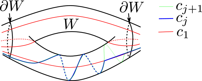
Figure 8. A choice of representatives of the homotopy classes $c_{j}$ and $c_{j+1}$.

It remains to show that the bound for $R$ can be chosen so that the subsurface in question contains an element of $A$ or a curve $t_{i}$. Recall the assumptions on the curves $c_{1}$ and $c_{n}$ in Lemma 28. Suppose $W$ is an essential subsurface of $S\setminus c$. If $d_{W}(c_{1},T_{c}^{j}(c_{j}))=3$ and $d_{W}(c_{1},T^{-k}_{c}(c_{k}))=5$ for $j<k$, then each connected component of $W\cap c_{j}$ can be decomposed into an arc lying along $c_{1}$ and an arc homotopic to a subarc of a connected component of $c_{k}\cap W$, see Figure 8. This is because otherwise $T^{-k}_{c}(c_{k})\cap W$ would have connected components corresponding to those of $T^{-j}_{c}(c_{j})\cap W$ that prevent $d_{W}(c_{1},T^{-k}_{c}(c_{k}))>4$. Similarly, if $d_{W}(c_{1},T^{-l}_{c}(c_{l}))=7$ for $k<l$, each connected component of $W\cap c_{j}$ can be decomposed into an arc lying along $c_{1}$ and an arc homotopic to a subarc of a connected component of $c_{l}\cap W$. Either $l-j$ can be chosen large enough to ensure that $t_{j},t_{j+1},\ldots,t_{l-1}$ are not all homotopic, or the subsurface $Y$ can be taken to be $\mathcal{A}_{t_{j}}$. If $t_{j},t_{j+1},\ldots,t_{l-1}$ are not all homotopic, by the argument given in the proof of Lemma 28, $W$ must contain an element of $A$. It follows that $R$ can be chosen large enough to guarantee that $D_{Y}(s_{3},B)\geq N$ for any $N\in\mathbb{N}$ and $Y$ contains a curve $t_{i}$ or an element of $A$.

5.6. Proof of Lemma 18

This subsection puts all the pieces together to give a proof of Lemma 18.

Lemma 31 (Lemma 18 from Subsection 5.1).

Suppose that $d(A,B)\geq 3$, and let $c$ be a simple curve, which is no longer assumed to be distance one from $A$. Then for all but finitely many $n\in\mathbb{Z}$,

$$d(A,D_{c}^{n}(B))\geq d(A,B)$$

Proof.

If $A$ and $B$ could each be shown to have finite diameter in the subsurface projection to $\mathcal{A}_{c}$, the theorem would follow from the same argument as for Lemma 20. By Theorem 21, this is the case for example when $d(c,A)\geq 2$ and $d(c,B)\geq 2$. This special case of the lemma was also proven in Theorem 1.4 of [17]. When $c$ is distance 1 from $A$, it follows that the theorem is true with $s_{2}$ in place of $A$.

Alternatively, if $D_{c}$ takes $A$ or $B$ to itself, e.g. $c\in B$ or $c\in A$, the theorem also follows. This implies that the theorem is true with $s_{1}$ in place of $A$.

The theorem will now be proven under the assumption that $d(c,A)=1$, $d(c,B)\geq 2$ and $d(A,B)\geq 3$. The argument in the case that $d(c,B)=1$, $d(c,A)\geq 2$ is symmetric. For this case, all that remains is to prove the theorem with $s_{3}$ in place of $A$.

Choose $\{a_{1},\ldots,a_{n}\}$ as usual, where $\{a_{m}\ldots,a_{n}\}$ are in $s_{2}$. By Lemma 22, there is an upper bound $L$ on the distance between $\{a_{1},\ldots,a_{n}\}$ and any curve in $B$ when projected to the subsurface $Y$ from Lemma 28. By Corollary 29 and the constraints on $R$ in the definition of $s_{2}$, this is true for all of $s_{2}$. It follows that for any $n$, a geodesic shorter than $d(A,B)$ from a vertex representing a curve in $D_{c}^{-n}(s_{3})$ to a vertex representing a curve in $B$ must pass through a vertex representing a curve disjoint from some $t_{i}$ or disjoint from an element of $A$.

In the latter case, it can be seen immediately that the geodesic can not be shorter than a geodesic from $A$ to $B$. In the former case, for a curve $s$ in $D_{c}^{-n}(s_{3})$, it will now be shown that $d(D_{c}^{-n}(s_{3}),B)\geq d(A,B)$. To understand why this is so, note that a geodesic from a curve in $D_{c}^{-n}(s_{3})$ to $B$ must pass through a vertex representing a curve disjoint from $t_{i}$, so the length of the geodesic is independent of the number of twists around $t_{i}$. Given a geodesic $\gamma$ from a curve $f_{n}$ in $D_{c}^{-n}(s_{3})$ to a vertex $b$ in $B$, this will be used to construct a path $\gamma^{{}^{\prime}}$ from a vertex $f$ in $A$ to the vertex $b$, that is no longer than $\gamma$.

Denote by $t$ the vertex on $\gamma$ representing a curve disjoint from $t_{i}$. The vertex $f$ in $A$ is obtained by starting with $D_{c}^{n}(f_{n})$. Assume initially that is is possible to perform $c$-twisting band sums on $D_{c}^{n}(f_{n})$ that twist around $t_{i}$ and $c$. These $c$-twisting band sums are performed in such a way as to obtain $f$, for which $d_{\mathcal{A}_{c}}(f,b)\leq 1$. The path $\gamma^{{}^{\prime}}$ is composed of two geodesic segments. One geodesic segment connects $f$ to a vertex $t^{{}^{\prime}}$, and the other connects $t^{{}^{\prime}}$ to $b$. If $t$ is disjoint from $c$, then $t^{{}^{\prime}}$ and $t$ coincide. Otherwise, $t^{{}^{\prime}}$ is obtained from $t$ by performing some number of Dehn twists around $c$, so as to minimise $d_{\mathcal{A}_{c}}(t^{{}^{\prime}},f)$ and hence also $d_{\mathcal{A}_{c}}(t^{{}^{\prime}},b)$. It follows that $d(f,t^{{}^{\prime}})\leq d(f_{n},t)$ and $d(t,b)\leq d(t^{{}^{\prime}},b)$, and the length of $\gamma^{{}^{\prime}}$ is less than or equal to that of $\gamma$, as claimed.

It remains to explain the construction of $\gamma^{{}^{\prime}}$ when it is not possible to perform $c$-twisting band sums on $D_{c}^{n}(d_{n})$ that twist around $t_{i}$ and $c$. This happens when $D_{c}^{n}(d_{n})$ intersects the curve $d_{i}$ involved in the $c$-twisting band sum. Using bigon surgery, decompose $D_{c}^{n}(f_{n})$ into a band sum of curves $\{g_{i}\}$, $i\in 1,\ldots,m$ disjoint from $d_{i}$, and attached along arcs $\{h_{i}\}$. This is done in such a way that only one of the curves in the band sum decomposition, call it $g_{1}$, intersects $c$. Perform the $c$-twisting band sums on $g_{1}$. Take band sums with the curves $\{g_{i}\},i=2,\ldots,m$, however, these band sums are now performed with arcs obtained from $\{h_{i}\}$ by twisting around $t_{i}$. This gives the curve $f$ in $A$. The path $\gamma^{{}^{\prime}}$ is now constructed as before. ∎

References

- [1] A. Casson and C. Gordon. Reducing Heegaard splittings. Topology and its Applications, 27(3):275–283, 1987.
- [2] R. Detcherry. Unpublished personal communication. 2019.
- [3] N. Dunfield and W. Thurston. Finite covers of random 3-manifolds. Inventiones Mathematicae, (3):457–521, 2006.
- [4] J. Hempel. 3-manifolds as viewed from the curve complex. Topology, 40(3):631–657, 2001.
- [5] N. Ivanov. Fifteen problems about the mapping class groups. In Problems on mapping class groups and related topics, volume 74 of Proceedings of Symposia in Pure Mathematics, pages 71–80. American Mathematical Society, Providence, RI, 2006.
- [6] J. Johnson. Notes on heegaard splittings. https://users.math.yale.edu/~jj327/notes.pdf.
- [7] D. Long and H. Morton. Hyperbolic -manifolds and surface automorphisms. Topology, 25(4):575–583, 1986.
- [8] A. Lubotzky, J. Maher, and C. Wu. Random methods in 3-manifold theory. Trudy Matematicheskogo Instituta Imeni V. A. Steklova. Rossiĭskaya Akademiya Nauk, 292(Algebra, Geometriya i Teoriya Chisel):124–148, 2016. Reprinted in Proceedings of the Steklov Instute of Mathematics 292 (2016), no. 1, 118–142.
- [9] J. Maher. Random walks on the mapping class group. Duke Mathematical Journal, 156(3):429–468, 2011.
- [10] H. Masur and Y. Minsky. Geometry of the complex of curves II: Hierarchical Structure. Geometric and Functional Analysis, 10, 2000.
- [11] H. Masur and S. Schleimer. The geometry of the disk complex. Journal of the American Mathematical Society, 26(1):1–62, 2013.
- [12] Y. Minsky. Curve complexes, surfaces and 3-manifolds. Proceedings of the International Congress of Mathematicians, 2006.
- [13] W. Neumann and D. Zagier. Volumes of hyperbolic three-manifolds. Topology, 24(3):307–332, 1985.
- [14] I. Rivin. Statistics of 3-manifolds occasionally fibering over the circle. Preprint 2014, arXiv:1401.5736v4.
- [15] I. Rivin. Generic phenomena in groups: some answers and many questions. In Thin groups and superstrong approximation, volume 61 of Publications of the Research Institute for Mathematical Sciences, pages 299–324. Cambridge Univ. Press, Cambridge, 2014.
- [16] R. Webb. Uniform bounds for bounded geodesic image theorems. Journal für die Reine und Angewandte Mathematik, 709:219–228, 2015.
- [17] M. Yoshizawa. High distance Heegaard splittings via Dehn twists. Algebraic and Geometric Topology, 14(2):979–1004, 2014.