Generalized Canonical Correlation Analysis:
A Subspace Intersection Approach

Abstract

Generalized Canonical Correlation Analysis (GCCA) is an important tool that finds numerous applications in data mining, machine learning, and artificial intelligence. It aims at finding ‘common’ random variables that are strongly correlated across multiple feature representations (views) of the same set of entities. CCA and to a lesser extent GCCA have been studied from the statistical and algorithmic points of view, but not as much from the standpoint of linear algebra. This paper offers a fresh algebraic perspective of GCCA based on a (bi-)linear generative model that naturally captures its essence. It is shown that from a linear algebra point of view, GCCA is tantamount to subspace intersection; and conditions under which the common subspace of the different views is identifiable are provided. A novel GCCA algorithm is proposed based on subspace intersection, which scales up to handle large GCCA tasks. Synthetic as well as real data experiments are provided to showcase the effectiveness of the proposed approach.

1 Introduction

Canonical Correlation Analysis (CCA) is a classical statistical tool for two-set / two-view factor analysis [1, 2]. It aims at extracting a common latent structure of a set of entities observed in two different feature domains, which are usually referred as the ‘views’ of the entities. For example, an English document and its French translation is an entity represented in two different language-views. CCA can be naturally extended to the multi-view case, where more than two views are available for processing. Then it is referred as generalized CCA (GCCA) or multi-view CCA (MCCA) [3]. CCA/GCCA can also be considered as an extension of principal component analysis (PCA) to the case where multiple views of the data are available. On the one hand PCA seeks for a feature representation that maximizes the variance explained, thus keeping the strong / principal feature components. On the other hand, CCA/GCCA extracts the common components between the views and ideally ignores even strong components that are not present in all the views.

(G)CCA is a powerful set of tools with diverse applications in machine learning [4, 5, 6, 7], data mining [8, 9, 10, 11], signal processing [12, 13, 14, 15, 16], biomedical engineering [17, 18, 19], heath care data analytics [20], and genetics [21, 22], among others.

In the two view case, CCA can be optimally solved via generalized eigenvalue decomposition [2]. Furthermore, several algorithms exist that solve the CCA problem when big and high dimensional datasets are involved, and eigenvalue solutions are computationally prohibitive, e.g., [23, 24]. The multi-view scenario, on the other hand, is more complicated. There exist a number of different GCCA formulations, e.g., SUMCOR, MAXVAR, SUQUAR, etc; see [25, 3], and the majority of them are not solvable in polynomial time. SUMCOR and MAXVAR are the most popular formulations and various algorithms have been developed for them, e.g., [9, 14, 20, 10, 11].

Although CCA and GCCA are well-known and broadly-used tools with a long history, there still exist intriguing questions and open challenges related to (G)CCA theory and practice. First, our understanding of CCA/GCCA from an algebraic perspective is limited. The majority of the literature focuses on the statistical interpretation of CCA, e.g., [1, 3, 26], where each view is considered as a set of random vector realizations, and/or on algorithmic aspects. Interpreting (G)CCA from an algebraic viewpoint is important, since in practice the matrix views involved in (G)CCA do not necessarily follow a statistical model. Second, identifiability of CCA/GCCA, i.e., conditions under which the common latent components can be recovered, has only been partially studied. An identifiability condition for CCA was derived in [16], but only for the two view case. Finally, there is limited analysis regarding the effect of multiple views compared to just using two views. Despite the rapid developments in data acquisition and cross-platform data availability, which enable leveraging multiple views of a given set of entities, researchers often work with just two views due to the more complicated nature of GCCA.

In this work we give answers to the above research questions. We show that from an algebraic point of view, GCCA amounts to subspace intersection, i.e., it computes the intersection of the subspaces of the given matrix views. Furthermore, we provide improved and general conditions under which the common subspace between the views is identifiable. Our conditions show that having access to more views which share a common subspace benefits the identifiability of that subspace. In addition, we propose a simple and effective subspace intersection algorithm for GCCA which works for any number of views greater than or equal to two. The algorithm is algebraic and it exploits knowledge of the desired rank (useful signal rank, i.e., the dimension of the dominant information-bearing ‘signal subspace’) of the matrix views. We also develop a large-scale approximation algorithm which works for big and high-dimensional data, both dense and sparse. Extensive simulations with synthetically generated and real datasets showcase the effectiveness of our proposed framework.

Notation: Vectors, matrices and subspaces are denoted by lower case boldface, upper case boldface and upper case italic respectively. The $r$-th column, transpose, Frobenius norm, rank, range and kernel of a matrix $\bm{A}$ are denoted by $\bm{a}_{r},~{}\bm{A}^{T},~{}\lVert\bm{A}\rVert_{F},~{}\text{rank}(\bm{A}),~{}\text{range}\left(\bm{A}\right),~{}\text{ker}(\bm{A})$, respectively. The symbol $\oplus$ denotes the direct sum between two subspaces, $\bigcap$ is the subspace intersection operator, $\mathit{B}^{\perp}$ is the orthogonal complement of subspace $\mathit{B}$ and $\text{dim}{({\mathit{B}})}$ denotes the dimension of subspace $\mathit{B}$.

2 GCCA data model

We begin our discussion by reviewing the classical CCA formulation [2, 5]:

$$\max_{\bm{Q}^{(1)},\bm{Q}^{(2)}} ~{}{\rm Tr}\left(\bm{Q}^{(1)T}\bm{X}^{(1)T}\bm{X}^{(2)}\bm{Q}^{(2)}\right)$$ (1a)

$${\rm s.t.} ~{}\bm{Q}^{(n)T}\bm{X}^{(n)T}\bm{X}^{(n)}\bm{Q}^{(n)}=\bm{I}_{R},~{}n=1,2,$$ (1b)

where $\bm{X}^{(n)}\in\mathbb{C}^{I\times K_{n}}$ is the $n$-th view containing $I$ entities measured in a $K_{n}$-dimensional feature space, $\bm{Q}^{(n)}\in\mathbb{C}^{K_{n}\times R}$ is a matrix that projects $\bm{X}^{(n)}$ onto a subspace of dimension $R$ and $\bm{I}_{R}$ represents the $R\times R$ identity matrix. The previous optimization form can be equivalently written as:

$$\min_{\bm{Q}^{(1)},\bm{Q}^{(2)}} ~{}\lVert\bm{X}^{(1)}\bm{Q}^{(1)}-\bm{X}^{(2)}\bm{Q}^{(2)}\rVert_{F}$$ (2a)

$${\rm s.t.} ~{}\bm{Q}^{(n)T}\bm{X}^{(n)T}\bm{X}^{(n)}\bm{Q}^{(n)}=\bm{I}_{R},~{}n=1,2.$$ (2b)

Therefore in the noiseless case the optimal CCA solution gives:

$$\bm{X}^{(1)}\bm{Q}^{(1)}=\bm{X}^{(2)}\bm{Q}^{(2)}$$ (3a)

$${\rm s.t.} ~{}\bm{Q}^{(n)T}\bm{X}^{(n)T}\bm{X}^{(n)}\bm{Q}^{(n)}=\bm{I}_{R},~{}n=1,2,$$ (3b)

Equivalently, when multiple views are considered, the solution in the noiseless case should satisfy:

$$\bm{X}^{(n_{1})}\bm{Q}^{(n_{1})}=\bm{X}^{({n_{2}})}\bm{Q}^{({n_{2}})},~{}n_{1}\neq n_{2}$$ (4a)

$${\rm s.t.} ~{}\bm{Q}^{(n)T}\bm{X}^{(n)T}\bm{X}^{(n)}\bm{Q}^{(n)}=\bm{I}_{R},~{}n,n_{1},n_{2}\in\{1,\dots,N\}$$ (4b)

It is straightforward to see that if (4a) holds then the range of the views $\bm{X}^{(1)},\ldots,\bm{X}^{(N)}$ share a common $R$-dimensional subspace and thus admit the following multi-view factorization:

$$\bm{X}^{(n)}=[\bm{M},\bm{C}^{(n)}]\bm{S}^{(n)T},\quad n\in\{1,\ldots,N\},$$ (5)

where $\bm{M}\in\mathbb{C}^{I\times R}$ is a shared factor matrix, while $\bm{C}^{(n)}\in\mathbb{C}^{I\times L_{n}}$ and $\bm{S}^{(n)}\in\mathbb{C}^{K_{n}\times(R+L_{n})}$ are individual matrices for all $n\in\{1,\ldots,N\}$. The goal of generalized CCA is to find the subspace $\text{range}(\bm{M})$, observing $\bm{X}^{(1)},\ldots,\bm{X}^{(N)}$. Note the factorization in (5) also holds for the standard two-view CCA, in which $N=2$.

As far as identifiability is concerned, [16] studied the two-view CCA and proved that if the matrices $[\bm{M},\bm{C}^{(1)},\bm{C}^{(2)}]$, $\bm{S}^{(1)}$ and $\bm{S}^{(2)}$ have full column rank, then $\text{range}\left(\bm{M}\right)$ can be obtained via CCA. In this paper we move a step forward and provide an identifiability condition for the general case of GCCA. More precisely, using the range subspace intersection approach for GCCA, we propose an identifiability condition that does not require any of the matrices in the set $\{[\bm{M},\bm{C}^{(n_{1})},\bm{C}^{(n_{2})}]\}$ to have full column rank.

Our first observation is that since $\bm{M}$ is a shared factor matrix, we can without loss of generality (w.l.o.g.) assume that the matrices $\{[\bm{M},\bm{C}^{(n)}]\}$ in (5) have full column rank (see Appendix A for detailed proof). Next, we assume for simplicity that the matrices $\{\bm{S}^{(n)}\}$ in (5) have full column rank. This assumption is used for brevity, although it is not generally necessary for identifiability of the common subspace. In the case where $\{\bm{S}^{(n)}\}$ matrices do not have full column rank, the analysis becomes more complicated and is reserved for future work. The full column rank property of $\{[\bm{M},\bm{C}^{(n)}]\}$ and the full column rank assumption on $\{\bm{S}^{(n)}\}$ allow us to assume, w.l.o.g. that

$$\text{range}(\bm{X}^{(n)})=\text{range}(\bm{M})\oplus\text{range}(\bm{C}^{(n)}),\quad n\in\{1,\ldots,N\},$$ (6)

which implies that

$$R\leq I-\max_{1\leq n\leq N}L_{n}.$$ (7)

Note that equation (6) is a key point of our approach and follows naturally from the fact that matrix $[\bm{M},\bm{C}^{(n)}]$ has full column rank and that the subspaces $\text{range}(\bm{M})$ and $\text{range}(\bm{C}^{(n)})$ are complementary (see Appendix A for details).

3 A range subspace intersection approach for generalized CCA

In this section we provide a range subspace intersection approach for finding $\text{range}\left(\bm{M}\right)$ via the observed matrices $\bm{X}^{(1)},\ldots,\bm{X}^{(N)}$. The full column rank assumptions on the matrices $\{[\bm{M},\bm{C}^{(n)}]\}$ and $\{\bm{S}^{(n)}\}$ in (5) imply that

$$\text{range}(\bm{X}^{(n_{1})})\cap\text{range}(\bm{X}^{(n_{2})})$$

$$=\text{range}([\bm{M},\bm{C}^{(n_{1})}])\cap\text{range}([\bm{M},\bm{C}^{(n_{2})}])$$

$$=\text{range}(\bm{M})+\left(\text{range}(\bm{C}^{(n_{1})})\cap\text{range}(\bm{C}^{(n_{2})})\right),$$

$$\hskip 150.00023pt1\leq n_{1}<n_{2}\leq N,$$

where the last equality follows from (6). More generally, we have that

$$Y :=\bigcap_{n=1}^{N}\text{range}(\bm{X}^{(n)})=\text{range}(\bm{M})+\bigcap_{n=1}^{N}\text{range}(\bm{C}^{(n)})$$

$$=\text{range}(\bm{M})\oplus\left(\bigcap_{n=1}^{N}\text{range}(\bm{C}^{(n)})\cap\text{range}(\bm{M})^{\perp}\right)$$

$$=\text{range}(\bm{M})\oplus C,$$ (8)

where $C:=\bigcap_{n=1}^{N}\text{range}\left(\bm{C}^{(n)}\right)\cap\text{range}(\bm{M})^{\perp}$. Observe that $\text{dim}(Y)=R$ implies that $Y=\text{range}(\bm{M})$. To put it differently, if the dimension of the subspace spanned by a basis for $Y$ is $R$-dimensional, then $\text{range}(\bm{M})$ can be uniquely determined from $Y$.

What remains to be answered is how to determine the dimension of $Y$. Consider a nonzero vector $\bm{z}\in\mathbb{C}^{I}$. Since the columns of $\bm{X}^{(n)}\in\mathbb{C}^{I\times(R+L_{n})}$ form a basis for $\text{range}(\bm{X}^{(n)})$, we know that $\bm{z}\in Y$ if and only if there exist nonzero vectors $\boldsymbol{q}^{(1)}\in\mathbb{C}^{R+L_{1}},\ldots,\boldsymbol{q}^{(N)}\in\mathbb{C}^{R+L_{N}}$ such that

$$\bm{z}=\bm{X}^{(1)}\boldsymbol{q}^{(1)}=\cdots=\bm{X}^{(N)}\boldsymbol{q}^{(N)}.$$ (9)

Define $\boldsymbol{q}=[\boldsymbol{q}^{(1)T},\ldots,\boldsymbol{q}^{(N)T}]^{T}\in\mathbb{C}^{(NR+\sum_{n=1}^{N}L_{n})}$. Then a vector $\boldsymbol{q}$ with property (9) can be obtained by solving the system of homogenous linear equations

$$\left[\bm{0}_{I,\alpha_{n_{1}}},\bm{X}^{(n_{1})},\bm{0}_{I,\beta_{n_{1},n_{2}}},-\bm{X}^{(n_{2})},\bm{0}_{I,\omega_{n_{2}}}\right]\boldsymbol{q}=\bm{0}_{I},$$ (10)

for $1\leq n_{1}<n_{2}\leq N$, where
$\alpha_{n_{1}}=(n_{1}-1)R+\sum_{i=1}^{n_{1}-1}L_{i}$,
$\beta_{n_{1},n_{2}}=(n_{2}-n_{1}-1)R+\sum_{i=n_{2}+1}^{n_{2}-1}L_{i}$,
$\omega_{n_{2}}=(N-n_{2})R+\sum_{i=n_{2}+1}^{N}L_{i}$.

We can now conclude that if the subspace

$$Z^{(N)}:={\bigcap_{1\leq n_{1}<n_{2}\leq N}\text{ker}([\bm{0},\bm{X}^{(n_{1})},\bm{0},-\bm{X}^{(n_{2})},\bm{0}])}$$

$$={\bigcap_{1\leq n_{1}<n_{2}\leq N}\text{ker}([\bm{0},\bm{M},\bm{C}^{(n_{1})},\bm{0},-\bm{M},-\bm{C}^{(n_{2})},\bm{0}}])$$ (11)

is $R$-dimensional, i.e., there exist only $R$ linearly independent vectors $\boldsymbol{q}^{(1)},\ldots,\boldsymbol{q}^{(N)}$ in the range of $Z^{(N)}$, then $Y$ is also $R$-dimensional and $Y=\text{range}(\bm{M})$. Note that the dimensions of the zero matrices in (11) are as in (10), but have been omitted due to space limitations.

Therefore the dimension of $Y$ can be expressed in terms of the factor matrices $\bm{M},\{\bm{C}^{(n)}\}_{n=1}^{N}$. For example, when $N=3$, the dimension of $Y$ is equal to the dimension of the kernel of the following matrix (the same reasoning holds true when $N>3$):

$$\left[\begin{array}[]{cccccc}\bm{M}&\bm{C}^{(1)}&-\bm{M}&-\bm{C}^{(2)}&\bm{0}&\bm{0}\\ \bm{M}&\bm{C}^{(1)}&\bm{0}&\bm{0}&-\bm{M}&-\bm{C}^{(3)}\\ \bm{0}&\bm{0}&\bm{M}&\bm{C}^{(2)}&-\bm{M}&-\bm{C}^{(3)}\end{array}\right].$$ (15)

4 Identifiability condition for generalized CCA

Since $\text{range}(\bm{M})\subseteq Y$, the minimal dimension of the subspace $Y$ given by (8) is $R$. This also means that if the subspace $Z^{(N)}$ given by (11) is $R$-dimensional, then $C=\{\bm{0}\}$. This fact leads to the common subspace identifiability condition presented in Theorem 4.1:

Theorem 4.1

Consider the multi-view factorization of $\bm{X}^{(1)},\ldots,\bm{X}^{(N)}$ given by (5). If

$$\left\{\begin{aligned} &Z^{(N)}\text{ is $R$-dimensional},\\ &\bm{S}^{(1)},\ldots,\bm{S}^{(N)}\text{ have full column rank},\end{aligned}\right.$$ (16)

then $\text{dim}\left(\bigcap_{n=1}^{N}\text{range}(\bm{X}^{(n)})\right)=R$
and  $\bigcap_{n=1}^{N}\text{range}(\bm{X}^{(n)})=\text{range}(\bm{M})$.

Note that checking the dimension of $Z^{(N)}$ in (16) can be cumbersome and it is not obvious how it is related to the factor matrices $\bm{M},\bm{C}^{(1)},\ldots,\bm{C}^{(N)}$ in (5). In order to obtain a simpler condition for the recovery of $\text{range}(\bm{M})$ via $\bm{X}^{(1)},\ldots,\bm{X}^{(N)}$, the following identity will be used [27]:

$$\text{dim}\left(\bigcap_{n=1}^{N}\text{range}(\bm{X}^{(n)})\right)$$

$$=\sum_{n=1}^{N}\text{rank}(\bm{X}^{(n)})-\text{rank}(\boldsymbol{\Gamma}(\bm{X}^{(1)},\ldots,\bm{X}^{(N)})),$$ (17)

where the matrix $\boldsymbol{\Gamma}(\bm{X}^{(1)},\ldots,\bm{X}^{(N)})$ is defined as follows:

$$\boldsymbol{\Gamma}(\bm{X}^{(1)},\ldots,\bm{X}^{(N)})=\left[\begin{array}[]{cccc}\bm{X}^{(1)}&-\bm{X}^{(2)}&&\\ \vdots&&\ddots&\\ \bm{X}^{(1)}&&&-\bm{X}^{(N)}\\ \end{array}\right],$$

in which $\bm{X}^{(1)},\ldots,\bm{X}^{(N)}$ are matrices of conformable sizes. Relation (4) together with the full column rank assumptions on $\bm{S}^{(1)},\ldots,\bm{S}^{(N)}$ imply that

$$\text{dim}\left(\bigcap_{n=1}^{N}\text{range}(\bm{X}^{(n)})\right)=$$

$$\sum_{n=1}^{N}\text{rank}(\bm{X}^{(n)})-\text{rank}(\boldsymbol{\Gamma}(\bm{X}^{(1)},\ldots,\bm{X}^{(N)}))=$$

$$\sum_{n=1}^{N}\text{rank}([\bm{M},\bm{C}^{(n)}])-\text{rank}(\boldsymbol{\Gamma}([\bm{M},\bm{C}^{(1)}],\ldots,[\bm{M},\bm{C}^{(N)}])).$$ (18)

The full column rank property of the matrices $[\bm{M},\bm{C}^{(1)}],\ldots,[\bm{M},\bm{C}^{(N)}]$ in turn imply that relation (18) simplifies to

$$\text{dim}\left(\bigcap_{n=1}^{N}\text{range}(\bm{X}^{(n)})\right)=$$

$$NR+\sum_{n=1}^{N}L_{n}-\text{rank}(\boldsymbol{\Gamma}([\bm{M},\bm{C}^{(1)}],\ldots,[\bm{M},\bm{C}^{(N)}]))$$

$$NR+\sum_{n=1}^{N}L_{n}-\text{rank}\left(\boldsymbol{\Gamma}^{(N)}\right),$$ (19)

where the matrix $\boldsymbol{\Gamma}^{(N)}\in\mathbb{C}^{(N-1)I\times((N-1)R+\sum_{n=1}^{N}L_{n})}$ in (19) is given by

$$\boldsymbol{\Gamma}^{(N)}=\left[\begin{array}[]{ccccc}\bm{C}^{(1)}&-\bm{M}&-\bm{C}^{(2)}&&\\ \vdots&&\ddots&\ddots&\\ \bm{C}^{(1)}&&&-\bm{M}&-\bm{C}^{(N)}\\ \end{array}\right].$$ (20)

From (19) it is clear that if $\boldsymbol{\Gamma}^{(N)}$ has full column rank, then $\text{dim}\left(\bigcap_{n=1}^{N}\text{range}(\bm{X}^{(n)})\right)=R$ and $\bigcap_{n=1}^{N}\text{range}(\bm{X}^{(n)})=\text{range}(\bm{M})$. Theorem 4.2 below summarizes the simplified version of the common subspace identifiability condition in Theorem 4.1.

Theorem 4.2

Consider the multi-set factorization of $\bm{X}^{(1)},\ldots,\bm{X}^{(N)}$ given by (5). If

$$\left\{\begin{aligned} &\boldsymbol{\Gamma}^{(N)}\text{ has full column rank},\\ &\bm{S}^{(1)},\ldots,\bm{S}^{(N)}\text{ have full column rank},\end{aligned}\right.$$ (21)

then $\text{dim}\left(\bigcap_{n=1}^{N}\text{range}\left(\bm{X}^{(n)}\right)\right)=R$
and  $\bigcap_{n=1}^{N}\text{range}\left(\bm{X}^{(n)}\right)=\text{range}\left(\bm{M}\right)$.

Note that if $\boldsymbol{\Gamma}^{(N)}$ has full column rank, then the matrices $[\bm{M},\bm{C}^{(1)}],\ldots,[\bm{M},\bm{C}^{(N)}]$ must also have full column rank.

Regarding necessary conditions so that (21) is satisfied, we have:

$$\left\{\begin{aligned} &R+\frac{1}{N-1}\sum_{n=1}^{N}L_{n}\leq I,\\ &R+L_{n}\leq K_{n},\quad n\in\{1,\ldots,N\}.\end{aligned}\right.$$ (22)

Now we consider the case where $\bm{M},\bm{C}^{(n)},\bm{S}^{(n)},n=1,\dots,N$ are generic. Then $R+L_{n}\leq K_{n}$ is also sufficient for $\bm{S}^{(n)}$ to have full column rank. In order to study the rank of $\boldsymbol{\Gamma}^{(N)}$, when $\bm{M},\bm{C}^{(n)},n=1,\dots,N$ are generic, we will make use of the following lemma:

Lemma 4.3

[28] Let $f:\mathbb{C}^{n}\to\mathbb{C}$ be an analytic function. If there exists an element $\bm{x}\in\mathbb{C}^{n}$ such that $f\left(\bm{x}\right)\neq 0$, then the set $\{\,\bm{x}\,|\,f\left(\bm{x}\right)=0\,\}$ is of Lebesgue measure zero.

Recall that an $m\times n$ matrix has full column rank $n$ if it has a non-vanishing $n\times n$ minor. Since a minor is an analytic function (namely, it is a multivariate polynomial), Lemma 4.3 can now be used to verify whether the matrices in (21) generically have full column rank. As a result, $R+\frac{1}{N-1}\sum_{n=1}^{N}L_{n}\leq I$ is generically sufficient for $\boldsymbol{\Gamma}^{(N)}$ to have full column rank, if there exists a single example of $\bm{M},\bm{C}^{(n)},n=1,\dots,N$ with det$\left(\boldsymbol{\Gamma}^{(N)}\right)\neq 0$ for each tuple $\{R,L_{1},\ldots,L_{N}\}$. An illustrative derivation of such an example for a special but interesting choice of $\{R,L_{1},\ldots,L_{N}\}$ is provided in the supplementary material. Numerical experiments indeed suggest that the conditions in (22) are generically sufficient for generalized CCA identifiability.

5 Further Discussion and Insights

In this section we discuss the effect of processing more views (i.e., $N>2$) using GCCA compared to the more commonly used CCA model in which $N=2$.

First we note that when $N=2$, condition (21) boils down to the standard two-view CCA identifiability condition obtained in [16]. However, when $N>2$ condition (21) yields relaxed identifiability. For example, consider the case where $\bm{M},\bm{C}^{(n)},\bm{S}^{(n)},n=1,\dots,N$ are generic and $R=L_{n}=100,~{}n=1,\dots,N$. Then condition (22) for two-view CCA requires $I\geq R+L_{1}+L_{2}=300$, in order to recover $\text{range}\left(\bm{M}\right)$. When $N=3$, however, the condition in (22) is relaxed to $I\geq R+\frac{1}{2}(L_{1}+L_{2}+L_{3})=250$. Furthermore, in the latter case none of the matrices $[\bm{M},\bm{C}^{(1)},\bm{C}^{(2)}]$, $[\bm{M},\bm{C}^{(1)},\bm{C}^{(3)}]$ and $[\bm{M},\bm{C}^{(2)},\bm{C}^{(3)}]$ are required to have full column rank, which is necessary in the two-view case. The identifiability condition for GCCA can be further relaxed by increasing $N$. In the previous example, when $N=5$ the condition in (22) reduces to $I\geq 225$ and as $N\to\infty$ to $I\geq R+L_{n}=200$, which is also a necessary condition to identify $\text{range}\left(\bm{M}\right)$.

Another important difference between the two-view and multi-view CCA is that when $N=2,~{}\text{range}\left(\bm{C}^{(1)}\right)\cap\text{range}\left(\bm{C}^{(2)}\right)=\{\bm{0}\}$ is a necessary identifiability condition. On the contrary, for $N>2$ it is possible that $\text{range}\left(\bm{C}^{(m)}\right)\cap\text{range}\left(\bm{C}^{(n)}\right)\neq\{\bm{0}\}$ for some $m\neq n$, i.e., some views are allowed to share common subspaces not included in $\text{range}\left(\bm{M}\right)$.

To further elaborate on the identifiability properties of CCA ($N=2$) and GCCA ($N>2$), consider the case where $R$ is fixed. Condition (22) implies that

$$\sum_{n=1}^{N}L_{n}\leq(N-1)(I-R)$$ (23)

is necessary for condition (21) to be satisfied. If additionally $L_{1}=\cdots=L_{N}$, then (23) reduces to:

$$L_{n}\leq\frac{N-1}{N}(I-R),$$ (24)

which yields the following relation, when $N=2$:

$$L_{n}\leq\frac{1}{2}(I-R).$$ (25)

From (24), we can also infer that in the asymptotic case where $N\to\infty$, (24) reduces to:

$$L_{n}\leq I-R.$$ (26)

Comparing (25) with (26), we conclude that in the balanced case where $L_{1}=\cdots=L_{N}$, GCCA can at most relax the CCA bound on $L_{n}$ by a factor two.

Let us now consider the balanced case ($L_{1}=\cdots=L_{N}$) where $L_{n}$ is fixed, while $R$ is varying. Relation (25) implies that CCA with $N=2$ views is able to recover the common subspace $\text{range}\left(\bm{M}\right)$ only if

$$R\leq I-2L_{n}.$$ (27)

In other words, $L_{n}<\frac{I}{2}$ is a necessary recovery condition for CCA. On the contrary, employing more views ($N>2$), allows GCCA to recover the common subspace $\text{range}\left(\bm{M}\right)$, even if $L_{n}\geq\frac{I}{2}$. For instance, if $I=200$, $N=5$ and $L_{1}=\cdots=L_{N}=100$, then it can be verified that condition (22) is satisfied as a long as $R\leq 75$, regardless of the fact that $L_{n}=\frac{I}{2}$. Furthermore, as $N\to\infty$ we get from (26) that:

$$R\leq I-L_{n}$$ (28)

is necessary to satisfy condition (21) in Theorem 4.2. Comparing (27) with (28), we conclude that when $L_{1}=\cdots=L_{N}$ and $L_{n}<\frac{I}{2}$, GCCA can at most relax the bound on $R$ by a factor of two. Moreover, when $L_{n}\geq\frac{I}{2}$, GCCA can still ensure the recovery of $\text{range}\left(\bm{M}\right)$ while this is never possible when $N=2$.

6 Algorithmic framework

In this section we develop an algebraic algorithm that uses a range subspace intersection approach to tackle the GCCA problem. The algorithm follows the previous analysis and can be viewed as a constructive interpretation of Theorem 4.1. It can be described in 3 steps:

step 1: We compute $\bm{U}_{n}\in\mathbb{C}^{I\times(R+L_{n})}$ and $\bm{V}_{n}\in\mathbb{C}^{K_{n}\times(R+L_{n})}$ whose columns form an orthonormal basis for $\text{range}\left(\bm{X}^{(n)}\right)$ and $\text{range}\left(\bm{X}^{(n)T}\right)$, $n\in\{1,\ldots,N\}$ respectively.
step 2: This step forms a matrix $\bm{\Theta}\in\mathbb{C}^{NI\times(NR+\sum_{n=1}^{N}L_{n})}$ and computes a basis for it’s nullspace, represented by matrix $\bm{\Phi}$. An example of matrix $\bm{\Theta}$ when $N=3$ can be found in (15). The columns of $\bm{\Phi}$ form an orthonormal basis for $Z^{(N)}$ in (11). Note that $\bm{\Phi}=[\bm{\Phi}^{(1)T},\ldots,\bm{\Phi}^{(N)T}]^{T}$, with $\bm{\Phi}^{(n)}\in\mathbb{C}^{(R+L_{n})\times R}$. Then the matrices $\bm{Q}^{(n)},~{}n=1,\dots,N$ that project each view $\bm{X}^{(n)}$ to the common subspace $\text{range}\left(\bm{M}\right)$ can be obtained as $\bm{Q}^{(n)}=\bm{V}_{n}\bm{\Phi}^{(n)}$.
step 3: We build matrix $\bm{G}=[\bm{U}^{(1)}\bm{\Phi}^{(1)},\ldots,\bm{U}^{(N)}\bm{\Phi}^{(N)}]$. Finally we compute matrix $\bm{M}$ whose columns form an orthonormal basis for $\text{range}\left(\bm{G}\right)$, which is the common subspace. The detailed steps can be found in Algorithm 1.

  Input: $\{\bm{X}^{(n)},L_{n}\}_{n=1}^{N},~{}R$.

  Output: $\bm{M},\bm{Q}^{(n)}$.

  step 1:

  for $n=1$ to $N$ do

     $\bm{U}_{n}\bm{\Sigma}_{n}\bm{V}_{n}^{T}\leftarrow{\rm svds}\left(\bm{X}^{(n)},^{\prime}R+L_{n}^{\prime}\right);$

  end for

  step 2:

  $\bm{\Theta}=[\cdot];$

  for $n_{1}=1$ to $N-1$ do

     for $n_{2}=n_{1}+1$ to $N$ do

        $k=(n_{1}-1)R+\sum_{1}^{n_{1}-1}L_{n},~{}l=(n_{2}-n_{1}-1)R+\sum_{1}^{n_{2}-n_{1}-1}L_{n},~{}m=(N-n_{2})R+\sum_{n_{2}}^{N}L_{n};$

        $\bm{\theta}_{n_{1}n_{2}}=[\bm{0}_{I\times k},\bm{U}_{n_{1}},\bm{0}_{I\times l},-U_{n_{2}},\bm{0}_{I\times m}];$

        $\bm{\Theta}=[\bm{\Theta};\bm{\theta}_{n_{1}n_{2}}];$

     end for

  end for

  $\bm{U}_{\theta}\bm{\Sigma}_{\theta}\bm{V}_{\theta}^{T}\leftarrow{\rm svd}\left(\bm{\Theta},^{\prime}{\rm econ}^{\prime}\right);$

  $\bm{\Phi}=\bm{V}_{\theta}(:,\text{end}-R+1:\text{end});$

  step 3:

  $\bm{G}=[\cdot];$

  for $n=1$ to $N$ do

     $k=(n-1)R+\sum_{1}^{n-1}L_{n},~{}l=nR+\sum_{1}^{n}L_{n};$

     $\bm{G}=[\bm{G},\bm{U}_{n}\bm{\Phi}(k+1:l,:)];$

     $\bm{Q}^{(n)}=\bm{V}_{n}\bm{\Phi}(k+1:l,:);$

  end for

  $\bm{U}_{m}\bm{\Sigma}_{m}\bm{V}_{m}^{T}\leftarrow{\rm svds}\left(\bm{G},^{\prime}R^{\prime}\right);$

  $\bm{M}=\bm{U}_{m};$

Algorithm 1 RAnge subspaCe INtersection for Gcca (RACING)

In terms of computational complexity and memory requirements, the main bottleneck of the proposed algorithm lies in step 1 and step 2. In particular, the dimension of the columnspace of each view $\bm{X}^{(n)}$ is usually large which makes the SVD computation in step 1 and step 2 very intensive. To be more precise, the number of flops required to perform the SVD in step 1 and step 2 are $\mathcal{O}(IK_{n}\min(I,K_{n}))$ and $\mathcal{O}(N(N-1)I(NR+\sum_{1}^{N}L_{n})^{2})$. To overcome this issue for high dimensional data we propose to choose $L_{n}$ such that $R+L_{n}$ represents the useful signal rank, i.e., the dimension of the signal subspace, which is small enough for every $n\in\{1,\dots,N\}$. Then Lanczos-type iterative algorithms [29] can be used to compute the truncated SVD that significantly reduce the computational complexity, especially when sparse data are involved and $R+L_{n}\ll I$. For example, choosing $R+L_{n}$ to be in the order of $500$ will allow the proposed algorithm to work for very large and high-dimensional data.

7 Experiments

In this section we demonstrate the performance of the proposed algorithmic framework and showcase it’s effectiveness in synthetic- and real-data experiments. All simulations are implemented in Matlab and are executed on a Linux server comprising 32 cores at 2GHz and 128GB RAM.

7.1 Synthetic-Data Experiments

First we test the proposed framework using experiments with synthetically generated data. The multiple views are generated according to equation (5). We assume that the views share a common latent factor ${\bm{M}}\in\mathbb{R}^{I\times R}$ with entries randomly and independently drawn from a zero-mean unit-variance Gaussian distribution. The individual matrices $\bm{C}^{(n)}\in\mathbb{C}^{I\times L_{n}}$ and $\bm{S}^{(n)}\in\mathbb{C}^{K_{n}\times(R+L_{n})}$ are also generated with entries independently drawn from a zero-mean unit-variance Gaussian distribution and for simplicity we set $L_{n}=L$ and $K_{n}=K=L+R$ for every $n\in\{1,\dots,N\}$.

We test the algorithm in a noisy setup. To be more specific, $\bm{X}^{(n)},~{}n=1,\dots,N$ are generated according to the model in (5), as previouly described. However, instead of $\bm{X}^{(n)}$ we observe $\bm{B}^{(n)},~{}n=1,\dots,N$ which are generated as: $\bm{B}^{(n)}=\bm{X}^{(n)}+\bm{W}^{(n)},~{}~{}~{}~{}n\in\{1,\dots,N\},$ where $\bm{W}^{(n)}$ is additive white Gaussian noise. Note that in the noiseless case the proposed algorithm is able to recover the common subspace exactly, for every tested scenario that satisfies the conditions in (22). For baselines we use the exact solution of MAXVAR formulation, computed via eigenvalue decomposition and CSR-BCD, which solves the SUMCOR formulation, using a change of variables and a block coordinate descent (BCD) approach [10]. To evaluate the performance, we observe the maximum angle between the generated common subspace and the estimated one as defined in [30, 31], i.e.,

$$\texttt{angle}\left(\bm{M}_{1},\hat{{\bm{M}_{1}}}\right)=\lVert\bm{P}_{1}-\hat{\bm{P}_{1}}\rVert_{2},$$ (29)

where ${\bm{P}_{1}}(\hat{\bm{P}_{1}})$ is the orthogonal projection onto $\bm{M}_{1}(\hat{{\bm{M}_{1}}})$.

In the experiments we consider $N=6$ different views, that share a common subspace of dimension $R=50$. Two scenarios are generated: In the first each view consists of $I=2000$ rows, and $L=1000$ that leads to $K=1050$ columns for each view, whereas in the second $I=2000$, $Q=500$ that leads to $K=550$ columns for each view. We test the algorithmic performance for different levels of signal-to-noise-ratio (SNR), which is defined as:

$$SNR=20\log\frac{\sum_{n=1}^{N}\lVert\bm{X}^{(n)}\rVert_{F}}{\sum_{n=1}^{N}\lVert\bm{W}^{(n)}\rVert_{F}}.$$

Fig. 1(a) shows the performance of the proposed RACING along the baselines for different levels of SNR in the first scenario. Note that each algorithm is implemented to utilize either all 6 views to identify the common space, or the first 2 views, denoted by the subscript next to the name of the algorithm. We observe that the proposed algorithm is able to identify the common subspace for a wide range of SNRs, when 6 views are utilized. On the contrary all algorithms fail to identify the correct subspace, when only 2 views are employed. Note that the identifiability condition in (22) yields $50+\frac{N}{N-1}1000\leq 2000$, which is satisfied for $N=6$ but fails when $N=2$.

In the second scenario we reduce the dimension of the columnspace of each view to $K=550$. In this case the identifiability condition in (22) yields $50+\frac{N}{N-1}500\leq 2000$, which is satisfied for both $N=6$ and $N=2$. The results are illustrated in Fig. 1(b). We observe that although the identifiability condition in (22) is satisfied in both cases where 2 and 6 views are utilized, the algorithms perform better in the 6-view implementation. From both experiments we can also deduce that the proposed RACING works similarly to the MAXVAR solution and significantly outperforms CSR-BCD. This is a notable, considering that both MAXVAR and CSR-BCD are optimization approaches and are expected to perform better in the presence of noise.

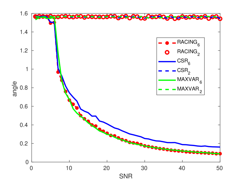
(a) First scenario

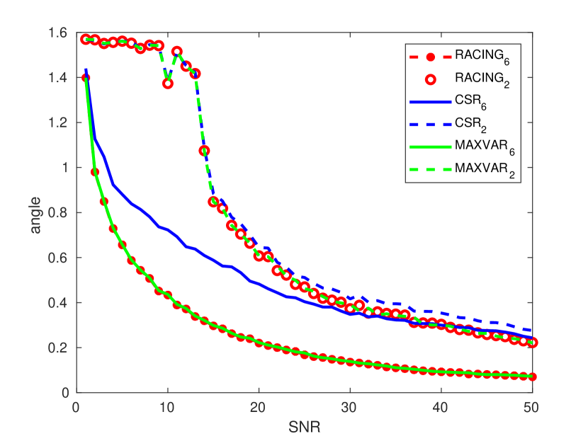
(b) Second scenario

Figure 1: Angle between true and recovered subspace.

Next we test the performance of the proposed approach and the baselines in the case where the views are approximately low rank. To this end, we generate ${\bm{M}},~{}\bm{C}^{(n)}$ as before in scenario 1 and 2 ($I=2000,~{}L=1000,~{}R=50,~{}K=1050$ and $I=2000,~{}L=500,~{}R=50,~{}K=550$ respectively), but this time we allow $\bm{X}^{(n)}$ to have low rank by letting $\bm{S}^{(n)}$ to be ‘fat matrices’, i.e., $\bm{S}^{(n)}\in\mathbb{C}^{K\times I}$. Note that we add noise as before, so the views are technically full rank, but when the noise is small they are approximately low-rank – i.e., they can be well-approximated by low-rank matrices. As mentioned earlier although our identifiability analysis used the full rank property of the views for simplicity, this is not in general necessary for identifiability and the subspace intersection framework. This is an important point, since although real data are typically full rank due to noise and measurement errors, the useful signal rank is often lower, and the remaining components are mostly noise. The results are presented in Fig. 2.

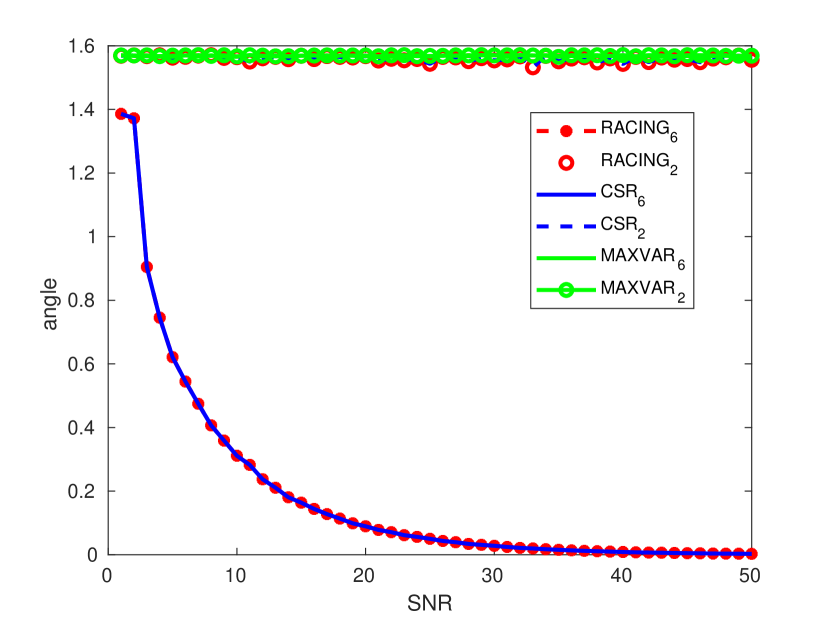
(a) First scenario with approximately low-rank views

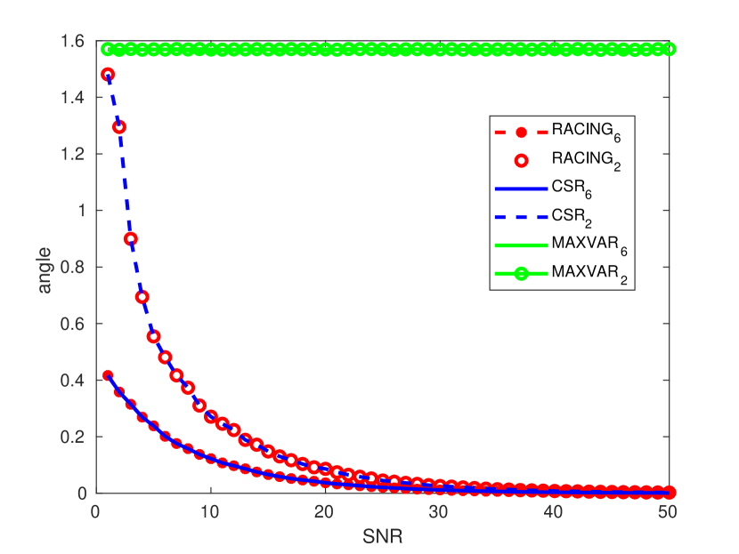
(b) Second scenario with approximately low-rank views

Figure 2: Angle between true and recovered subspace.

It is clear from Fig. 2 that approximately low-rank views do not affect the performance of CSR and the proposed RACING. However, MAXVAR formulations fail to identify the common subspace. This can be explained from the fact that MAXVAR analysis and algorithm assume that the views are effectively full rank as mentioned earlier. On the contrary, the proposed RACING is allows prescribing the useful signal rank of each view, as does CSR. Overall, in our experiments RACING works better than CSR and comparably to MAXVAR in the full-rank scenarios, whereas in the low-rank scenarios it markedly outperforms MAXVAR and works similarly to CSR.

7.2 Cross Language information Retrieval

Finally, we test the proposed approach on the task of cross language information retrieval (CLIT). Given a set of sentences along with their translations in multiple languages the goal is to learn a low-dimensional subspace where the sentences and their translations are maximally correlated. Then, new high-dimensional sentences are projected onto the associated lower dimensional space in order to determine their translation through a database of possible choices. Note that CLIT allows fast query and search across languages, which is beneficial to machine translation systems [32, 33, 34].

Data: The dataset employed is the Europarl parallel corpus [35]. It contains a collection of sentences translated in 21 European languages: Romanic (French, Italian, Spanish, Portuguese, Romanian), Germanic (English, Dutch, German, Danish, Swedish), Slavik (Bulgarian, Czech, Polish, Slovak, Slovene), Finni-Ugric (Finnish, Hungarian, Estonian), Baltic (Latvian, Lithuanian), and Greek. In our experiments we only focus on the Germanic languages, i.e., English, Dutch, German, Danish and Swedish. Each sentence is represented by a high-dimensional ‘bag of words’ vector with $K_{n}=524,288$ features.

Procedure: We choose a training and testing set of $I=134,227$ and $I_{t}=38,352$ sentences in each language-view respectively. In the training phase, the GCCA algorithms are applied to the training set in order to learn $\bm{Q}^{(n)},~{}n=1,\ldots,N$ that project each sentence to a common low dimensional subspace. In the testing phase, the testing sentences across all languages are projected onto the lower dimensional space after multiplication with $\bm{Q}^{(n)},~{}n=1,\ldots,N$. The CLIT task is completed by matching the query sentences with their translations, according to their distances in the low-dimensional subspace.

We consider 2 scenarios. In the first one, training and testing are performed using only $N=2$ languages, i.e., Dutch and Danish. In the second scenario, the training and testing phase takes into account all Germanic languages (Dutch, Danish, English, German, Swedish).

Evaluation: The baseline algorithms used for comparison are MVLSA [9], that approximately solves the MAXVAR criterion and GCCA-PDD [11], which is a primal-dual algorithm that tackles the SUMCOR formulation for sparse large-scale data. We initialize GCCA-PDD, with RACING and ran for 25 iterations (total number of 5 inner and 5 outer iterations).

To measure the performance of the competing algorithms we use the AROC and NN-freq. metric as defined in [11]. The first is a ranking metric for the position of the correct translation, whereas NN-freq. measures the probability of the correct translation to be in the first place.
Results: Table I shows the performance of the competing algorithms for the two scenarios of CLIT. The dimension of the subspace where each sentence is projected is $R=70$ and $L_{n}=230$ for all views. Regarding GCCA-PDD, the $\rho$ parameter is set equal to 2. One can see that the CLIT task significantly benefits by incorporating multiple languages. To be more precise, both metrics show performance improvement when all Germanic languages are employed. For example RACING achieves an improvement of approximately $10\%$ in NN freq. and $1.2\%$ in AROC, when all Germanic languages are used. Note that the difference in AROC is also significant since for $N=5$ the right translation ranks in the top $290$ position, whereas for $N=2$ only in the top $520$ position. Furthermore, we observe that $PDD-GCCA$ initialized by RACING outperforms the other two methods, whereas RACING works better than MVLSA.

TABLE I: Average AROC and NN freq. (both in %) of the Danish-Dutch CLIT.

	metric	# of languages
Algorithm		Danish-Dutch	5 Germanic languages
PDD-GCCA	AROC	97.36	98.56
	NN freq.	46.34	69.05
RACING	AROC	97.36	98.49
	NN freq.	46.34	56.97
MVLSA	AROC	96.20	97.06
	NN freq.	36.72	41.15

8 Conclusion

In this paper we studied generalized CCA from a linear algebraic perspective. In particular, we showed that GCCA can be interpreted as subspace intersection and provided identifiability conditions for recovering the common subspace between the views, which are relaxed compared to the standard two-view CCA. We also developed a range subspace intersection algorithm to perform GCCA, which can also handle large and high-dimensional datasets. Numerical experiments demonstrated the effectiveness of the proposed approach in the context of multi-view learning.

Appendix A Proof of equation (6)

In order to prove equation (6) we first need to prove that the following properties hold without loss of generality:

Property 1: $\bm{M}$, $\bm{C}^{(1)},\ldots,\bm{C}^{(N)}$ have full column rank. Without loss of generality we can assume that the matrices $\bm{M}\in\mathbb{C}^{I\times R},\bm{C}^{(1)}\in\mathbb{C}^{I\times L_{1}},\ldots,\bm{C}^{(N)}\in\mathbb{C}^{I\times L_{N}}$ in (5) all have full column rank, Indeed, if the columns of $\bm{M}$ are linearly dependent, then $\bm{M}$ can replaced by any subset of its columns that form a basis for $\text{range}(\bm{M})$ and the matrix ${\bf S}^{(n)}$ can be adjusted accordingly, without changing ${\bf X}^{(n)}$. (Similarly for $\bm{C}^{(1)},\ldots,\bm{C}^{(N)}$).

Property 2: $[\bm{M},\bm{C}^{(1)}],\ldots,[\bm{M},\bm{C}^{(N)}]$ have full column rank. First, note that the column dimension ($R+L_{n}$) of $[\bm{M},\bm{C}^{(n)}]$ should not exceed its row dimension $I$, i.e., $I\geq R+L_{n}$. Indeed, if $I<R+L_{n}$, then $R+L_{n}-I$ columns of $\bm{C}^{(n)}$ can be written as linear combinations of the other $I$ columns in $[\bm{M},\bm{C}^{(n)}]$. Therefore these $R+L_{n}-I$ columns of $\bm{C}^{(n)}$ could be discarded, while accordingly adjusting matrix ${\bf S}^{(n)}$, without changing ${\bf X}^{(n)}$. Furthermore, we can w.l.o.g. assume that $\text{range}(\bm{M})\cap\text{range}(\bm{C}^{(n)})=\{\bm{0}\}$, $n\in\{1,\ldots,N\}$, i.e., we assume w.l.o.g. that $\bm{c}_{q}^{(n)}\notin\text{range}(\bm{M})$, $q\in\{1,\ldots,L_{n}\}$, $n\in\{1,\ldots,N\}$. Indeed, if $\bm{c}_{t}^{(n)}=\bm{M}\boldsymbol{\beta}$ for some $\boldsymbol{\beta}\in\mathbb{C}^{R}$, then

$$\bm{X}^{(n)}=\sum_{r=1}^{R}\bm{m}_{r}\bm{s}_{r}^{(n)T}+\sum_{q=1}^{L_{n}}\bm{c}_{q}^{(n)}\bm{s}_{r}^{(n)T}=$$

$$\sum_{r=1}^{R}\bm{m}_{r}(\bm{s}_{r}^{(n)T}+\beta_{r}\bm{s}_{R+t}^{(n)T})+\sum_{\begin{subarray}{c}q=1\\ q\neq t\end{subarray}}^{L_{n}}\bm{c}_{q}^{(n)}\bm{s}_{r}^{(n)T}.$$ (30)

In other words, if $\bm{c}_{q}^{(n)}\in\text{range}(\bm{M})$, then we can simply consider a factorization of $\bm{X}^{(n)}$, as in (30), that only involves a smaller $I$-by-$(L_{n}-1)$ matrix $\bm{C}^{(n)}$. Now since $\text{range}(\bm{M})\cap\text{range}(\bm{C}^{(n)})=\{\bm{0}\}$, $n\in\{1,\ldots,N\}$ and $\bm{M},~{}\bm{C}^{(n)}$ have full column rank, we conclude that w.l.o.g. $[\bm{M},\bm{C}^{(n)}]$ has full column rank. Then relation (6) follows naturally from the fact that matrix $[\bm{M},\bm{C}^{(n)}]$ has full column rank and that the subspaces $\text{range}(\bm{M})$ and $\text{range}(\bm{C}^{(n)})$ are complementary.

Supplementary Material

In this section we provide an illustrative example of matrix $\boldsymbol{\Gamma}^{(N)}$ that has full column rank for an interesting choice of $\{R,L_{1},\ldots,L_{N}\}$. This implies that if $\bm{M},\bm{C}^{(n)},\bm{S}^{(n)},n=1,\dots,N$ are generic, then for this specific tuple that satisfies the equations in (19), $\boldsymbol{\Gamma}^{(N)}$ is full column rank, $\text{dim}\left(\bigcap_{n=1}^{N}\text{range}\left(\bm{X}^{(n)}\right)\right)=R$ and  $\bigcap_{n=1}^{N}\text{range}\left(\bm{X}^{(n)}\right)=\text{range}\left(\bm{M}\right)$. This follows our analysis in section 4. In other words, given that for this specific choice of $\{R,L_{1},\ldots,L_{N}\}$ we can find an example of $\boldsymbol{\Gamma}^{(N)}$ that has full column rank, det($\boldsymbol{\Gamma}^{(N)}$) is nontrivial and any generic set of matrices $\bm{M},\bm{C}^{(n)},\bm{S}^{(n)},n=1,\dots,N$ produces a matrix $\boldsymbol{\Gamma}^{(N)}$ that has full column rank with probability 1.

Consider the special case where $I=22$, $R=10$, $N=3$ and $L:=L_{1}=L_{2}=L_{3}$. Since $2I\geq 2R+3L$, we know that $L\leq\lfloor\frac{2}{3}(I-R)\rfloor=8$ is necessary. Hence, for the special case where $I=22$, $R=10$, $N=3$ and $L:=L_{1}=L_{2}=L_{3}=8$ it suffices to find a single set of matrices $\bm{M}\in\mathbb{C}^{I\times R}$, $\bm{C}^{(1)}\in\mathbb{C}^{I\times L},\bm{C}^{(2)}\in\mathbb{C}^{I\times L}$, $\bm{C}^{(3)}\in\mathbb{C}^{I\times L}$ in which $I=22$, $R=10$ and $L=8$ such that the matrix

$$\boldsymbol{\Gamma}^{(3)}=\left[\begin{array}[]{ccccc}\bm{C}^{(1)}&-\bm{M}&-\bm{C}^{(2)}&\bm{0}_{I,R}&\bm{0}_{I,L}\\ \bm{C}^{(1)}&\bm{0}_{I,R}&\bm{0}_{I,L}&-\bm{M}&-\bm{C}^{(3)}\end{array}\right]$$ (31)

has full column rank.

The overall idea is to set $[\bm{C}^{(1)},-\bm{M}]$ equal to the first $L+R$ columns of the $I\times I$ identity matrix $\bm{I}_{I}$, i.e., $[\bm{C}^{(1)},-\bm{M}]=\bm{I}_{I}(:,1:L+R)$ and then find appropriate (zero-one) matrices $-\bm{C}^{(2)}$ and $-\bm{C}^{(3)}$ such that $\boldsymbol{\Gamma}^{(3)}$ has full column rank. To be more precise let $\bm{C}^{(1)}=\bm{I}_{I}(:,1:L)$, $\bm{M}=\begin{bmatrix}\bm{0}_{I-R-L/2\times R}\\ \bm{I}_{R\times R}\\ \bm{0}_{L/2\times R}\end{bmatrix}$, $\bm{C}^{(2)}=\begin{bmatrix}\bm{0}_{L/2,L}\\ \bm{0}_{L/2,L/2},\bm{I}_{L/2}\\ \bm{0}_{I-L\times L}\\ \bm{I}_{L/2},\bm{0}_{L/2,L/2}\end{bmatrix}$, $\bm{C}^{(3)}=\begin{bmatrix}\bm{0}_{L/2,L/2},\bm{I}_{L/2}\\ \bm{0}_{R\times L}\\ \bm{I}_{L/2},\bm{0}_{L/2,L/2}\end{bmatrix}$. The resulting $\boldsymbol{\Gamma}^{(3)}$ is depicted bellow. Then by inspection of the matrix it is not hard to see that $\boldsymbol{\Gamma}^{(3)}$ has full column rank.

$\boldsymbol{\Gamma}^{(3)}=$ $\left[\begin{array}[]{cccccccccccccccccccccccccccccccccccccccccccc}1&&&&&&&&&&&&&&&&&&&&&&&&&&&&&&&&&&&&&&&&&&&\\ &1&&&&&&&&&&&&&&&&&&&&&&&&&&&&&&&&&&&&&&&&&&\\ &&1&&&&&&&&&&&&&&&&&&&&&&&&&&&&&&&&&&&&&&&&&\\ &&&1&&&&&&&&&&&&&&&&&&&&&&&&&&&&&&&&&&&&&&&&\\ &&&&1&&&&&&&&&&&&&&&&&&1&&&&&&&&&&&&&&&&&&&&&\\ &&&&&1&&&&&&&&&&&&&&&&&&1&&&&&&&&&&&&&&&&&&&&\\ &&&&&&1&&&&&&&&&&&&&&&&&&1&&&&&&&&&&&&&&&&&&&\\ &&&&&&&1&&&&&&&&&&&&&&&&&&1&&&&&&&&&&&&&&&&&&\\ &&&&&&&&1&&&&&&&&&&&&&&&&&&&&&&&&&&&&&&&&&&&\\ &&&&&&&&&1&&&&&&&&&&&&&&&&&&&&&&&&&&&&&&&&&&\\ &&&&&&&&&&1&&&&&&&&&&&&&&&&&&&&&&&&&&&&&&&&&\\ &&&&&&&&&&&1&&&&&&&&&&&&&&&&&&&&&&&&&&&&&&&&\\ &&&&&&&&&&&&1&&&&&&&&&&&&&&&&&&&&&&&&&&&&&&&\\ &&&&&&&&&&&&&1&&&&&&&&&&&&&&&&&&&&&&&&&&&&&&\\ &&&&&&&&&&&&&&1&&&&&&&&&&&&&&&&&&&&&&&&&&&&&\\ &&&&&&&&&&&&&&&1&&&&&&&&&&&&&&&&&&&&&&&&&&&&\\ &&&&&&&&&&&&&&&&1&&&&&&&&&&&&&&&&&&&&&&&&&&&\\ &&&&&&&&&&&&&&&&&1&&&&&&&&&&&&&&&&&&&&&&&&&&\\ &&&&&&&&&&&&&&&&&&1&&&&&&&&&&&&&&&&&&&&&&&&&\\ &&&&&&&&&&&&&&&&&&&1&&&&&&&&&&&&&&&&&&&&&&&&\\ &&&&&&&&&&&&&&&&&&&&1&&&&&&&&&&&&&&&&&&&&&&&\\ &&&&&&&&&&&&&&&&&&&&&1&&&&&&&&&&&&&&&&&&&&&&\\ 1&&&&&&&&&&&&&&&&&&&&&&&&&&&&&&&&&&&&&&&&1&&&\\ &1&&&&&&&&&&&&&&&&&&&&&&&&&&&&&&&&&&&&&&&&1&&\\ &&1&&&&&&&&&&&&&&&&&&&&&&&&&&&&&&&&&&&&&&&&1&\\ &&&1&&&&&&&&&&&&&&&&&&&&&&&&&&&&&&&&&&&&&&&&1\\ &&&&1&&&&&&&&&&&&&&&&&&&&&&&&&&&&&&&&&&&&&&&\\ &&&&&1&&&&&&&&&&&&&&&&&&&&&&&&&&&&&&&&&&&&&&\\ &&&&&&1&&&&&&&&&&&&&&&&&&&&&&&&&&&&&&&&&&&&&\\ &&&&&&&1&&&&&&&&&&&&&&&&&&&&&&&&&&&&&&&&&&&&\\ &&&&&&&&&&&&&&&&&&&&&&&&&&1&&&&&&&&&&&&&&&&&\\ &&&&&&&&&&&&&&&&&&&&&&&&&&&1&&&&&&&&&&&&&&&&\\ &&&&&&&&&&&&&&&&&&&&&&&&&&&&1&&&&&&&&&&&&&&&\\ &&&&&&&&&&&&&&&&&&&&&&&&&&&&&1&&&&&&&&&&&&&&\\ &&&&&&&&&&&&&&&&&&&&&&&&&&&&&&1&&&&&&&&&&&&&\\ &&&&&&&&&&&&&&&&&&&&&&&&&&&&&&&1&&&&&&&&&&&&\\ &&&&&&&&&&&&&&&&&&&&&&&&&&&&&&&&1&&&&&&&&&&&\\ &&&&&&&&&&&&&&&&&&&&&&&&&&&&&&&&&1&&&&&&&&&&\\ &&&&&&&&&&&&&&&&&&&&&&&&&&&&&&&&&&1&&&&&&&&&\\ &&&&&&&&&&&&&&&&&&&&&&&&&&&&&&&&&&&1&&&&&&&&\\ &&&&&&&&&&&&&&&&&&&&&&&&&&&&&&&&&&&&1&&&&&&&\\ &&&&&&&&&&&&&&&&&&&&&&&&&&&&&&&&&&&&&1&&&&&&\\ &&&&&&&&&&&&&&&&&&&&&&&&&&&&&&&&&&&&&&1&&&&&\\ &&&&&&&&&&&&&&&&&&&&&&&&&&&&&&&&&&&&&&&1&&&&\end{array}\right]$

References

- [1] H. Hotelling, “Relations between two sets of variants,” Biometrika, vol. 28, no. 3–4, pp. 321–377, 1936.
- [2] G. H. Golub and H. Zha, “The canonical correlations of matrix pairs and their numerical computation,” IMA Vol. Math. Appl,, vol. 69, pp. 27–49, 1995.
- [3] J. R. Kettenring, “Canonical analysis of several sets of variables,” Biometrika, vol. 58, no. 3, pp. 433–451, 1971.
- [4] A. Vinokourov, J. J. Shawe-Taylor, and N. Cristianini, “Inferring a semantic representation of text via cross-language correlation analysis,” in Proc. NIPS 2003, December 11-13, 2003, Whistler, British Columbia, Canada.
- [5] D. R. Hardoon, S. Szedmak, and J. Shawe-Taylor, “Canonical Correlation Analysis: An overview with application to learning methods,” Neural Computation, vol. 16, pp. 2639–2664, Dec. 2004.
- [6] P. Dhillon, D. Foster, and L. Ungar, “Multi-view learning of word embeddings via CCA,” in Proc. NIPS 2011, December 12-17, 2011, Granada, Spain.
- [7] G. Andrew, R. Arora, J. Bilmes, and K. Livescu, “Deep canonical correlation analysis,” in Proceedings of the 30th International Conference on Machine Learning, (Atlanta, Georgia, USA), pp. 1247–1255, 17–19 Jun 2013.
- [8] S. Bickel and T. Scheffer, “Multi-view clustering.,” in ICDM, vol. 4, pp. 19–26, 2004.
- [9] P. Rastogi, B. Van Durme, and R. Arora, “Multiview lsa: Representation learning via generalized cca.,” in HLT-NAACL, pp. 556–566, 2015.
- [10] X. Fu, K. Huang, E. E. Papalexakis, H.-A. Song, P. P. Talukdar, N. D. Sidiropoulos, C. Faloutsos, and T. Mitchell, “Efficient and distributed algorithms for large-scale generalized canonical correlations analysis,” in Data Mining (ICDM), 2016 IEEE 16th International Conference on, pp. 871–876, IEEE, 2016.
- [11] C. I. Kanatsoulis, X. Fu, N. D. Sidiropoulos, and M. Hong, “Structured sumcor multiview canonical correlation analysis for large-scale data,” IEEE Transactions on Signal Processing, vol. 67, pp. 306–319, Jan 2019.
- [12] J. Vía, I. Santamaría, and J. Pérez, “Deterministic CCA-based algorithms for blind equalization of FIR-MIMO channels,” IEEE Transactions on Signal Processing, vol. 55, July 2007.
- [13] S. Van Vaerenbergh, J. Vía, and I. Santamaría, “Blind identification of SIMO Wiener systems based on kernel canonical correlation analysis,” IEEE Transactions on Signal Processing, vol. 61, pp. 2219–2230, May 2013.
- [14] R. Arora and K. Livescu, “Multi-view learning with supervision for transformed bottleneck features,” in Proc. ICASSP 2014, pp. 2499–2503, 2014.
- [15] J. Manco-Vásquez, S. Van Vaerenbergh, J. Vía, and I. Santamaría, “Kernel canonical correlation analysis for robust cooperative spectrum sensing in cognitive radio networks,” Transactions on Emerging Telecommunications Technologies, vol. 28, 2014.
- [16] M. Ibrahim and N. D. Sidiropoulos, “Cell-edge interferometry: Reliable detection of unknown cell-edge users via canonical correlation analysis,” in Proc. IEEE SPAWC, July 2-5, 2019, Cannes, France., 2019.
- [17] M. Borga and H. Knutsson, “A canonical correlation approach to blind source separation,” Tech. Rep. LiU-IMT-EX-0062, Department of Biomedical Engineering, Linköping University, Linköping, Sweden,, 2001.
- [18] W. De Clercq, A. Vergult, B. Vanrumste, W. Van Paesschen, and S. Van Huffel, “Canonical correlation analysis applied to remove muscle artifacts from the electroencephalogram,” IEEE Transactions on Biomedical Engineering, vol. 53, pp. 2583–2587, Nov 2006.
- [19] C. Campi, L. Parkkonen, R. Hari, and A. Hyvärinen, “Non-linear canonical correlation for joint analysis of meg signals from two subjects,” Frontiers in Brain Imaging Methods, vol. 7, 2013.
- [20] J. C. Vasquez-Correa, J. R. Orozco-Arroyave, R. Arora, E. Nöth, N. Dehak, H. Christensen, F. Rudzicz, T. Bocklet, M. Cernak, H. Chinaei, et al., “Multi-view representation learning via gcca for multimodal analysis of parkinson” s disease,” in Proceedings of 2017 IEEE International Conference on Acoustics, Speech, and Signal Processing (ICASSP 2017), no. EPFL-CONF-224545, 2017.
- [21] E. Parkhomenko, D. Tritchler, J. Beyene, et al., “Sparse canonical correlation analysis with application to genomic data integration,” Statistical Applications in Genetics and Molecular Biology, vol. 8, no. 1, pp. 1–34, 2009.
- [22] D. M. Witten and R. J. Tibshirani, “Extensions of sparse canonical correlation analysis with applications to genomic data,” Statistical applications in genetics and molecular biology, vol. 8, no. 1, pp. 1–27, 2009.
- [23] Y. Lu and D. P. Foster, “Large scale canonical correlation analysis with iterative least squares,” in Advances in Neural Information Processing Systems, pp. 91–99, 2014.
- [24] R. Ge, C. Jin, P. Netrapalli, A. Sidford, et al., “Efficient algorithms for large-scale generalized eigenvector computation and canonical correlation analysis,” in International Conference on Machine Learning, pp. 2741–2750, 2016.
- [25] J. D. Carroll, “Generalization of canonical correlation analysis to three or more sets of variables,” in Proceedings of the 76th annual convention of the American Psychological Association, vol. 3, pp. 227–228, 1968.
- [26] F. R. Bach and M. I. Jordan, “A probabilistic interpretation of canonical correlation analysis,” 2005.
- [27] Y. Tiann, “The dimension of intersection of subspaces,” Missouri J. Math. Sci., vol. 14, no. 2, 2002.
- [28] R. C. Gunning and H. Rossi, Analytic Functions in Several Complex Variables. Prentice-Hall, 1965.
- [29] R. M. Larsen, “Lanczos bidiagonalization with partial reorthogonalization,” DAIMI Report Series, no. 537, 1998.
- [30] P. Å. Wedin, “On angles between subspaces of a finite dimensional inner product space,” in Matrix Pencils, pp. 263–285, Springer, 1983.
- [31] G. H. Golub and C. F. Van Loan, Matrix computations, vol. 3. JHU Press, 2012.
- [32] L. Ballesteros and W. B. Croft, “Phrasal translation and query expansion techniques for cross-language information retrieval,” in ACM SIGIR Forum, vol. 31, pp. 84–91, ACM, 1997.
- [33] J.-Y. Nie, M. Simard, P. Isabelle, and R. Durand, “Cross-language information retrieval based on parallel texts and automatic mining of parallel texts from the web,” in Proceedings of the 22nd annual international ACM SIGIR conference on Research and development in information retrieval, pp. 74–81, ACM, 1999.
- [34] W. Y. Zou, R. Socher, D. Cer, and C. D. Manning, “Bilingual word embeddings for phrase-based machine translation,” in Proceedings of the 2013 Conference on Empirical Methods in Natural Language Processing, pp. 1393–1398, 2013.
- [35] P. Koehn, “Europarl: A parallel corpus for statistical machine translation,” in MT summit, vol. 5, pp. 79–86, 2005.