Advanced Newton methods for geodynamical models of Stokes flow with viscoplastic rheologies

Abstract

Strain localization and resulting plasticity and failure play an important role in the evolution of the lithosphere. These phenomena are commonly modeled by Stokes flows with viscoplastic rheologies. The nonlinearities of these rheologies make the numerical solution of the resulting systems challenging, and iterative methods often converge slowly or not at all. Yet accurate solutions are critical for representing the physics. Moreover, for some rheology laws, aspects of solvability are still unknown. We study a basic but representative viscoplastic rheology law. The law involves a yield stress that is independent of the dynamic pressure, referred to as von Mises yield criterion. Two commonly used variants, perfect/ideal and composite viscoplasticity, are compared. We derive both variants from energy minimization principles, and we use this perspective to argue when solutions are unique. We propose a new stress–velocity Newton solution algorithm that treats the stress as an independent variable during the Newton linearization but requires solution only of Stokes systems that are of the usual velocity–pressure form. To study different solution algorithms, we implement 2D and 3D finite element discretizations, and we generate Stokes problems with up to 7 orders of magnitude viscosity contrasts, in which compression or tension results in significant nonlinear localization effects. Comparing the performance of the proposed Newton method with the standard Newton method and the Picard fixed-point method, we observe a significant reduction in the number of iterations and improved stability with respect to problem nonlinearity, mesh refinement, and the polynomial order of the discretization.

1 Introduction

Numerical simulations are important for understanding models of lithosphere dynamics over long time scales. These models are often non-Newtonian and include nonlinear mechanisms that can initiate norm faults [18, 31], strike-slip faults [32], and shear zones for subduction [25, 20, 34] through strain localization. This is commonly achieved by incorporating a form of frictional plasticity [27, 8, 2]. The transition from viscous to plastic behavior is controlled by stress-limiting techniques using a yield stress, whose value commonly depends on temperature and (lithostatic) pressure. The resulting nonlinear models take the form of incompressible Stokes equations and require numerical approximations of their solutions that have to be accurate and reliable. Obtaining accurate numerical solutions of models with plasticity is computationally challenging, however, because of the nonlinearities in the resulting systems [33, 6, 26, 17]. For instance, it can be difficult to obtain converged solutions where the (nonlinear) residual of the system has been reduced sufficiently. Moreover, these solutions strongly depend on the discretization, such as the refinement of the computational mesh.

In this paper, we study the solvability of viscoplastic Stokes flow in theory and with numerical experiments. Our main contribution is the development of nonlinear iterative methods with fast convergence that are, in addition, robust with respect to the severe nonlinearities of viscoplastic rheologies and problem discretizations. By solvability we refer to the existence of a unique solution of the flow problem; and convergence in this context means the rate of reduction of the (nonlinear) residual per iteration. While a plethora of models exist that involve plasticity, we focus on a moderately complex but representative and challenging rheological relation that switches from viscous to plastic flow at a yield stress. The considered yield stresses may vary spatially but do not depend on the dynamic pressure and thus not on the flow solution. The resulting law is sometimes referred to as von Mises rheology. This law can be generalized in multiple directions, such as to models that include elasticity, which naturally introduces a time scale and thus requires time stepping. The resulting systems exhibit solvability properties similar to problems without elasticity, but they tend be computationally less challenging and therefore converge to a solution sufficiently fast using standard nonlinear solvers [6]. Another generalization of viscoplastic models is to problems where the yield stress depends on the dynamic pressure that is part of the unknown solution, also called Drucker–Prager models [33, 26]. While these models are theoretically and computationally more complicated, they share several challenges with von Mises plasticity models, where the yield stress is independent of the solution.

The available iterative methods for nonlinear Stokes problems can be roughly divided into two categories: Picard-type or fixed-point methods, and Newton-type methods. It is well documented that Picard methods for nonlinear Stokes equations can be slow to converge and may result in poorly approximated numerical solutions, even after hundreds of iterations. Convergence typically degrades with the “severity” of the nonlinearity, and rheologies involving plasticity are particularly difficult because of their nonsmoothness. Thus, in recent years, researchers have been forced either to use simpler rheology laws or to consider more complex Newton-type or combined Picard–Newton methods [33, 9, 16, 6, 23]. In each iteration of a Newton-type method, a linearized system of equations is solved numerically to compute a Newton step, which is subsequently used to improve the current numerical approximation of the nonlinear system’s solution. The derivation and implementation of the linearized system require derivatives/Jacobians, which can potentially capture the nonlinear behavior better than Picard methods can, leading to faster convergence. For the viscoplastic rheologies we target, however, standard Newton methods still exhibit slow convergence, which worsens with finer computational meshes. Therefore, to advance the body of research on nonlinear methods for geophysical flows, we propose a novel Newton-type method that requires solution of Newton linearizations of the same computational complexity as standard Newton methods have, and with similar properties, but that demonstrates significantly improved convergence properties. We also derive structural properties of non-Newtonian viscoplastic flow models that we consider relevant for geodynamics. In particular, we show that underlying two commonly used laws for viscoplasticity is a minimization problem. This, in turn, provides a path to solvability, where we show the uniqueness of the solutions by arguing that they correspond to the unique minimizers of a strictly convex energy functional.

The overall time to solution for a nonlinear Stokes problem comprises the time for iterations of the nonlinear solver and for solution of the linearized systems in each nonlinear step. Hence, linear iterative methods and preconditioners for large-scale computational geophysics are important and rich research topics. The development and implementation of fast and scalable parallel linear solvers for three-dimensional Stokes problems have been addressed by us [28, 29, 16, 30] and others [21, 9, 22]. In this paper, however, we focus on nonlinear solvers and refer the reader to the above literature for numerically solving the linearized systems. We present the governing equations in Section 2 and show how a viscoplastic flow problem can be derived from energy minimization principles. In Section 3 we discuss what this implies for the uniqueness of solutions and the need for regularization. Section 4 presents iterative Newton-type algorithms, including our novel modified Newton algorithm, in which we treat the stress as an independent variable in the Newton linearization but still solve a system only in the standard velocity–pressure variables. We use two- and three-dimensional benchmark problems presented in Section 5 to numerically study solution features and to compare the convergence properties of the proposed solution method with existing approaches. The results of these comparisons are presented in Section 6.

2 Governing Equations

We consider nonlinear incompressible Stokes equations on a domain $\Omega\subset\mathbb{R}^{d}$, $d=2,3$, given by

$$-\nabla\cdot\bigl{[}\mu(\boldsymbol{u},p)\,(\nabla\boldsymbol{u}+\nabla\boldsymbol{u}^{\mathsf{T}})\bigr{]}+\nabla p =\boldsymbol{f}, \quad\text{in }\Omega,$$ (1a)

$$-\nabla\cdot\boldsymbol{u} =0, \quad\text{in }\Omega,$$ (1b)

where $\boldsymbol{u}$ and $p$ are the velocity and pressure fields, respectively; the right-hand side volumetric force is denoted by $\boldsymbol{f}$; and the effective viscosity, $\mu$, may depend on the pressure as well as on the second invariant of the strain rate tensor $\dot{\varepsilon}_{\textsc{ii}}^{\boldsymbol{u}}\coloneqq(\frac{1}{2}\,\dot{\boldsymbol{\varepsilon}}(\boldsymbol{u}):\dot{\boldsymbol{\varepsilon}}(\boldsymbol{u}))^{1/2}$, where “:” represents the inner product of second-order tensors and $\dot{\boldsymbol{\varepsilon}}(\boldsymbol{u})\coloneqq\frac{1}{2}(\nabla\boldsymbol{u}+\nabla\boldsymbol{u}^{\mathsf{T}})$ is the strain rate tensor. We assume that (1) is complemented with appropriate boundary conditions that, in particular, do not allow for arbitrary shifts or rotations in the velocity field. For the discussions in this paper, we further assume that $\mu=\mu(\boldsymbol{u})$, that is, the viscosity does not depend on the (dynamic) pressure. Instead, we focus on a nonsmooth strain-rate dependent constitutive relation that includes a yield stress, sometimes called the von Mises criterion [36, 10, 24, 33]. In particular, we consider two effective viscosity laws for viscoplastic flow,

$$\mu_{i}(\boldsymbol{u}) \coloneqq\underline{\mu}+\min\left(\frac{\tau_{\mathrm{y}}}{2\dot{\varepsilon}_{\textsc{ii}}^{\boldsymbol{u}}},{\mu_{\mathrm{r}}}\right),$$ (2a)

$$\mu_{c}(\boldsymbol{u}) \coloneqq\frac{\tau_{\mathrm{y}}{\mu_{\mathrm{r}}}}{2\dot{\varepsilon}_{\textsc{ii}}^{\boldsymbol{u}}{\mu_{\mathrm{r}}}+\tau_{\mathrm{y}}}.$$ (2b)

These constitutive relations incorporate plastic yielding with yield stress $\tau_{\mathrm{y}}>0$ and a reference viscosity ${\mu_{\mathrm{r}}}>0$. Additionally, (2a) incorporates a lower bound on the viscosity $\underline{\mu}\geq 0$, which plays a role in showing that solutions with (2a) are unique. Both the reference viscosity and the yield stress can be functions of ${\boldsymbol{x}}$. In geophysical applications, ${\mu_{\mathrm{r}}}$ may depend on a spatially varying temperature field, and the yield stress may depend on both temperature and pressure. We refer to (2a) as ideal and to (2b) as composite rheology for von Mises viscoplasticity. The composite rheology law is sometimes preferred because it avoids the pointwise $\min$-function and thus has better differentiability properties. Note that $\mu_{c}$ can also be written as a scaled harmonic mean, namely, $\mu_{c}(\boldsymbol{u})=({2\dot{\varepsilon}_{\textsc{ii}}^{\boldsymbol{u}}}/{\tau_{\mathrm{y}}}+1/{\mu_{\mathrm{r}}})^{-1}$, showing the relation between (2b) and (2a). As part of this paper, we will also discuss theoretical and practical differences between these two laws.

Next, we illustrate that (2a) and (2b) model a viscoplastic fluid with the von Mises yield criterion; in other words, they model a fluid with a yield stress. Let us first consider (2a), and introduce the stress tensor $\boldsymbol{\tau}\coloneqq 2\min\left({\tau_{\mathrm{y}}}/{(2\dot{\varepsilon}_{\textsc{ii}}^{\boldsymbol{u}})},{\mu_{\mathrm{r}}}\right)\dot{\boldsymbol{\varepsilon}}(\boldsymbol{u})$, which allows us to write (1a) in the form

$$-\nabla\cdot\bigl{[}2\underline{\mu}\dot{\boldsymbol{\varepsilon}}(\boldsymbol{u})+\boldsymbol{\tau}\bigr{]}+\nabla p =\boldsymbol{f}.$$ (3)

The definition of $\boldsymbol{\tau}$ implies that the second invariant of the stress tensor satisfies

$$\tau_{\textsc{ii}}=2\min\left(\frac{\tau_{\mathrm{y}}}{2\dot{\varepsilon}_{\textsc{ii}}^{\boldsymbol{u}}},{\mu_{\mathrm{r}}}\right)\dot{\varepsilon}_{\textsc{ii}}^{\boldsymbol{u}}\leq\tau_{\mathrm{y}}.$$ (4)

Hence, $\tau_{\textsc{ii}}$ is bounded by the yield stress, and if $\underline{\mu}=0$, (2a) models a von Mises rheology with either constant or spatially varying (e.g., depth-dependent) yield stress. The parameter $\underline{\mu}\geq 0$ is a regularization parameter such that ${\mu_{\mathrm{r}}}\gg\underline{\mu}$ and plays an important role in proving uniqueness of a solution of (1) with (2a).

Let us now consider the composite rheology model (2b), which is commonly used in geophysical applications. Defining the viscous stress tensor as $\boldsymbol{\tau}\coloneqq 2\mu_{c}\dot{\boldsymbol{\varepsilon}}(\boldsymbol{u})$, one can easily show that the second invariant of the corresponding strain rate tensor satisfies $\tau_{\textsc{ii}}\leq\tau_{\mathrm{y}}$; that is, it is again bounded by the yield stress.

The rheologies (2a) and (2b) can be generalized in several directions. One straightforward generalization is to make ${\mu_{\mathrm{r}}}$ a function of $\dot{\varepsilon}_{\textsc{ii}}^{\boldsymbol{u}}$, modeling non-Newtonian behavior in addition to the one caused by the yield stress. For instance, polynomial shear thinning is commonly used in mantle or ice flow [35, 15] models. The results in this paper can be generalized to these cases, and the only reason we do discuss models that incorporate both shear thinning and yielding is clarity of presentation. In our mantle flow simulation models [28, 29], we combine these two rheological phenomena, generalizing the approach presented in this paper. If the yield stress depends on the pressure, the effective viscosity laws (2a) and (2b) are known as Drucker–Prager rheologies.

3 Optimization Formulation

Here, we characterize the solutions to the incompressible Stokes equations with either (2a) or (2b) as minimizers of an appropriately chosen energy functional. The analogous result for the linear Stokes equations is well known [1], namely, that the linear Stokes solution minimizes a quadratic viscous energy functional over a space of sufficiently regular divergence-free vector functions. For simplicity, here we assume that the Stokes systems are combined with homogeneous Dirichlet boundary conditions on the entire boundary of the domain $\partial\Omega$. Other boundary conditions, such as free-slip conditions, can be used as long as they eliminate the null space of the Stokes operator, that is, exclude translations or rotations from the solution space [7].

To state the energy functional for the Stokes problem (1) and (2), we first define continuously differentiable functions $\varphi:\mathbb{R}_{\geq 0}\to\mathbb{R}$ representing ideal and composite viscoplasticity as follows:

$$\varphi_{i}(\sigma) \coloneqq\begin{cases}2{\mu_{\mathrm{r}}}\sigma^{2}+\dfrac{\tau_{\mathrm{y}}^{2}}{2{\mu_{\mathrm{r}}}}&\text{ if }2{\mu_{\mathrm{r}}}\sigma\leq\tau_{\mathrm{y}},\\ 2\tau_{\mathrm{y}}\sigma&\text{ else,}\end{cases}$$ (5a)

$$\varphi_{c}(\sigma) \coloneqq 2\tau_{\mathrm{y}}\sigma-\dfrac{\tau_{\mathrm{y}}^{2}}{{\mu_{\mathrm{r}}}}\log(\tau_{\mathrm{y}}+2{\mu_{\mathrm{r}}}\sigma),$$ (5b)

where as before we assume ${\mu_{\mathrm{r}}},\tau_{\mathrm{y}}>0$. Graphs of these functions are given in Figure 1 for illustration. We consider the energy minimization

$$\min_{\nabla\cdot{{\boldsymbol{u}}}=0}\Phi({\boldsymbol{u}}),\quad\Phi({{\boldsymbol{u}}})\coloneqq\int_{\Omega}\varphi(\dot{\varepsilon}_{\textsc{ii}}^{\boldsymbol{u}})\,d{\boldsymbol{x}}+2\underline{\mu}\int_{\Omega}(\dot{\varepsilon}_{\textsc{ii}}^{\boldsymbol{u}})^{2}\,d{\boldsymbol{x}}-\int_{\Omega}\boldsymbol{f}\cdot{{\boldsymbol{u}}}\,d{\boldsymbol{x}},$$ (6)

where $\varphi$ can be either $\varphi_{i}$ or $\varphi_{c}$. In the former case, in which we consider the function corresponding to the ideal law (5a), we assume $\underline{\mu}\geq 0$. In the case in which we consider the composite rheology function $\varphi=\varphi_{c}$, we always assume $\underline{\mu}=0$ such that the quadratic term in $\Phi(\cdot)$ vanishes. The minimization in (6) is over all divergence-free functions ${{\boldsymbol{u}}}\in H_{0}^{1}(\Omega)^{d}$. Here, the function space $H_{0}^{1}(\Omega)^{d}$ contains square-integrable functions that have square-integrable derivatives and that (for simplicity) satisfy homogeneous Dirichlet boundary conditions on $\partial\Omega$.

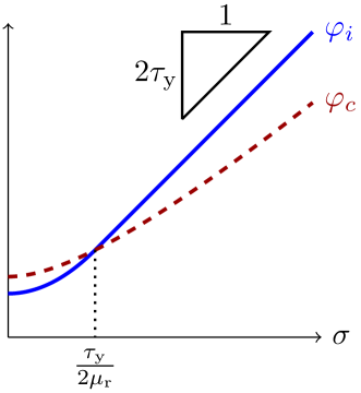
Figure 1: Sketch of functions $\varphi_{i}$ and $\varphi_{c}$ for ideal and composite viscoplasticity, respectively, as defined in (5). The function $\varphi_{i}$ consists of a quadratic and a linear piece, which are joined at $\sigma=\tau_{\mathrm{y}}/(2{\mu_{\mathrm{r}}})$. Both functions approach a slope of $2\tau_{\mathrm{y}}$ as $\sigma\to\infty$.

Next, we compute the first-order necessary conditions for (6), that is, the conditions a minimizer of (6) must satisfy. For that purpose, we use an arbitrary divergence-free velocity ${\boldsymbol{v}}\in H_{0}^{1}(\Omega)^{d}$ that satisfies the same homogeneous boundary condition as ${{\boldsymbol{u}}}$. Recall that the variation of $\dot{\varepsilon}_{\textsc{ii}}^{{\boldsymbol{u}}}$ with respect to ${\boldsymbol{u}}$ in a direction ${\boldsymbol{v}}$ is given by

$$[\delta_{{{\boldsymbol{u}}}}\dot{\varepsilon}_{\textsc{ii}}^{{\boldsymbol{u}}}]({\boldsymbol{v}})=\biggl{[}\delta_{{{\boldsymbol{u}}}}\sqrt{\tfrac{1}{2}\,\dot{\boldsymbol{\varepsilon}}(\boldsymbol{u}):\dot{\boldsymbol{\varepsilon}}(\boldsymbol{u})}\biggr{]}({\boldsymbol{v}})=\frac{\dot{\boldsymbol{\varepsilon}}({\boldsymbol{u}}):\dot{\boldsymbol{\varepsilon}}({\boldsymbol{v}})}{2\dot{\varepsilon}_{\textsc{ii}}^{{\boldsymbol{u}}}}.$$ (7)

Here and in the following, $\delta_{\boldsymbol{u}}$ denotes the variation with respect to $\boldsymbol{u}$. For the variation of $\Phi$ at ${\boldsymbol{u}}$ in direction ${\boldsymbol{v}}$, using the chain rule and (7), we obtain

$$[\delta_{{{\boldsymbol{u}}}}\Phi({{\boldsymbol{u}}})]({\boldsymbol{v}})=\int_{\Omega}\varphi^{\prime}(\dot{\varepsilon}_{\textsc{ii}}^{{\boldsymbol{u}}})\frac{\dot{\boldsymbol{\varepsilon}}({\boldsymbol{u}}):\dot{\boldsymbol{\varepsilon}}({\boldsymbol{v}})}{2\dot{\varepsilon}_{\textsc{ii}}^{{\boldsymbol{u}}}}\,d{\boldsymbol{x}}+\int_{\Omega}2\underline{\mu}\left(\dot{\boldsymbol{\varepsilon}}({\boldsymbol{u}}):\dot{\boldsymbol{\varepsilon}}({\boldsymbol{v}})\right)\,d{\boldsymbol{x}}-\int_{\Omega}\boldsymbol{f}\cdot{\boldsymbol{v}}\,d{\boldsymbol{x}}.$$ (8)

Taking the derivatives of (5a) and (5b), we have

$$\varphi_{i}^{\prime}(\sigma) =\left.\begin{cases}4{\mu_{\mathrm{r}}}\sigma&\text{ if }2{\mu_{\mathrm{r}}}\sigma<\tau_{\mathrm{y}}\\ 2\tau_{\mathrm{y}}&\text{ if }2{\mu_{\mathrm{r}}}\sigma>\tau_{\mathrm{y}}\end{cases}\right\}=2\min(2{\mu_{\mathrm{r}}}\sigma,\tau_{\mathrm{y}}),$$ (9)

$$\varphi_{c}^{\prime}(\sigma) =\frac{4{\mu_{\mathrm{r}}}\tau_{\mathrm{y}}\sigma}{2{\mu_{\mathrm{r}}}\sigma+\tau_{\mathrm{y}}},$$ (10)

we obtain for the integrands in (8)

$$\varphi_{i}^{\prime}(\dot{\varepsilon}_{\textsc{ii}}^{{\boldsymbol{u}}})\frac{\dot{\boldsymbol{\varepsilon}}({\boldsymbol{u}}):\dot{\boldsymbol{\varepsilon}}({\boldsymbol{v}})}{2\dot{\varepsilon}_{\textsc{ii}}^{{\boldsymbol{u}}}} =\left[\min\left(2{\mu_{\mathrm{r}}},\dfrac{\tau_{\mathrm{y}}}{\dot{\varepsilon}_{\textsc{ii}}^{{\boldsymbol{u}}}}\right)\right]\dot{\boldsymbol{\varepsilon}}({\boldsymbol{u}}):\dot{\boldsymbol{\varepsilon}}({\boldsymbol{v}}),$$

$$\varphi_{c}^{\prime}(\dot{\varepsilon}_{\textsc{ii}}^{{\boldsymbol{u}}})\dfrac{\dot{\boldsymbol{\varepsilon}}({\boldsymbol{u}}):\dot{\boldsymbol{\varepsilon}}({\boldsymbol{v}})}{2\dot{\varepsilon}_{\textsc{ii}}^{{\boldsymbol{u}}}} =\left[\dfrac{2{\mu_{\mathrm{r}}}\tau_{\mathrm{y}}}{2{\mu_{\mathrm{r}}}\dot{\varepsilon}_{\textsc{ii}}^{{\boldsymbol{u}}}+\tau_{\mathrm{y}}}\right]\dot{\boldsymbol{\varepsilon}}({\boldsymbol{u}}):\dot{\boldsymbol{\varepsilon}}({\boldsymbol{v}}).$$

Hence, the necessary optimality condition, $[\delta_{{{\boldsymbol{u}}}}\Phi({{\boldsymbol{u}}})]({\boldsymbol{v}})=0$ for all admissible ${\boldsymbol{v}}$, is the variational form of the the strong form of the Stokes problem (1), (2). The strong form can be recovered using integration by parts and the fact that ${\boldsymbol{v}}$ is arbitrary and by introducing the pressure as a Lagrange multiplier for the divergence-free condition [1].

Note that the optimization functional (6) is convex, which makes it useful for arguing existence and uniqueness of solutions. In particular if $\underline{\mu}>0$, the Stokes problem (1) and (2), combined with appropriate boundary conditions, has a unique solution since the energy functional $\Phi$ in (6) is strictly convex. While for $\underline{\mu}=0$ existence of solutions can be argued, they are not necessarily unique. Additionally, since the Stokes solution corresponds to a minimum of $\Phi$, this energy functional can also be used in a line search procedure to guarantee descent (and thus convergence) of iterative methods for nonlinear systems, such as a Newton or Picard method.

4 Standard and Stress–Velocity Newton Methods

Common methods for solving nonlinear systems of equations of the form (1) are the Picard fixed-point method and Newton’s method, or combinations thereof [24, 28, 9, 21, 6, 11, 33, 23]. As discussed in the preceding section, these iterative methods can be seen either as solving the nonlinear Stokes equations (1) or as minimizing the energy functional (6). Both iterative approaches are summarized next, where our derivations initially use an unspecified (convex) function $\varphi$ as in (6). At the end of this section, we list the standard and the stress–velocity Newton’s methods in Algorithm 1 as well as the specific linearized systems for ideal viscoplasticity $\varphi=\varphi_{i}$ in Table 1 and for composite viscoplasticity $\varphi=\varphi_{c}$ in Table 2.

4.1 Picard and standard Newton methods

The Picard fixed-point iteration for (1) and (2) starts with an initial guess $(\boldsymbol{u}_{0},p_{0})$ for velocity and pressure and, given an iterate $(\boldsymbol{u}_{k-1},p_{k-1})$, computes the next iterate $(\boldsymbol{u}_{k},p_{k})$ for $k=1,2,\ldots$ as solution to

$$-\nabla\cdot\left[\left(2\underline{\mu}+\frac{\varphi^{\prime}(\dot{\varepsilon}_{\textsc{ii}}^{{\boldsymbol{u}}_{k-1}})}{2\dot{\varepsilon}_{\textsc{ii}}^{{\boldsymbol{u}}_{k-1}}}\right)\dot{\boldsymbol{\varepsilon}}({\boldsymbol{u}_{k}})\right]+\nabla p_{k} =\boldsymbol{f},$$ (11a)

$$-\nabla\cdot\boldsymbol{u}_{k} =0,$$ (11b)

where $\dot{\varepsilon}_{\textsc{ii}}^{{\boldsymbol{u}}_{k-1}}$ is computed from the ($k-1$)st iterate. The new iterate depends only on the previous velocity and not on the pressure since the pressure variable enters linearly and acts as the Lagrange multiplier for enforcing the divergence-free condition. The Picard fixed-point method requires, in each iteration, the solution of one linear Stokes equation with spatially varying but isotropic viscosity. It typically converges from any initialization $(\boldsymbol{u}_{0},p_{0})$, but often exhibits slow convergence, in particular in the presence of significantly nonlinear or nonsmooth viscosity laws such as (2).

An alternative to the Picard iteration is Newton’s method, which, starting from an initial velocity–pressure pair $(\boldsymbol{u}_{0},p_{0})$, computes iterates by first solving the linear Newton system for the Newton update $(\tilde{}\boldsymbol{u},\tilde{p})$:

$$-\nabla\cdot\left[2\underline{\mu}\dot{\boldsymbol{\varepsilon}}(\tilde{\boldsymbol{u}})+\frac{\varphi^{\prime}(\dot{\varepsilon}_{\textsc{ii}}^{{\boldsymbol{u}}_{k-1}})}{2\dot{\varepsilon}_{\textsc{ii}}^{{\boldsymbol{u}}_{k-1}}}\bigg{(}\mathbb{I}-\psi(\dot{\varepsilon}_{\textsc{ii}}^{{\boldsymbol{u}}_{k-1}})\dfrac{\dot{\boldsymbol{\varepsilon}}(\boldsymbol{u}_{k-1})\otimes\dot{\boldsymbol{\varepsilon}}(\boldsymbol{u}_{k-1})}{2(\dot{\varepsilon}_{\textsc{ii}}^{{\boldsymbol{u}}_{k-1}})^{2}}\bigg{)}\dot{\boldsymbol{\varepsilon}}(\tilde{\boldsymbol{u}})\right]+\nabla\tilde{p} =-{\boldsymbol{r}}^{\boldsymbol{u}}_{k-1},$$ (12a)

$$-\nabla\cdot\tilde{{\boldsymbol{u}}} =-r^{p}_{k-1},$$ (12b)

where we use the notation

$$\psi(\dot{\varepsilon}_{\textsc{ii}}^{{\boldsymbol{u}}_{k-1}})\coloneqq\dfrac{\varphi^{\prime}(\dot{\varepsilon}_{\textsc{ii}}^{{\boldsymbol{u}}_{k-1}})-\dot{\varepsilon}_{\textsc{ii}}^{{\boldsymbol{u}}_{k-1}}\varphi^{\prime\prime}(\dot{\varepsilon}_{\textsc{ii}}^{{\boldsymbol{u}}_{k-1}})}{\varphi^{\prime}(\dot{\varepsilon}_{\textsc{ii}}^{{\boldsymbol{u}}_{k-1}})}.$$ (12c)

This is followed by the Newton update with step length $\alpha\leq 1$:

$$\boldsymbol{u}_{k}=\boldsymbol{u}_{k-1}+\alpha\tilde{}\boldsymbol{u},\quad p_{k}=p_{k-1}+\alpha\tilde{p},$$ (13)

which for $\alpha=1$ amounts to a so-called full Newton step. In (12a), $\mathbb{I}$ is the 4th-order identity tensor, and “$\otimes$” is the outer product between two (second-order) strain rate tensors. In the derivation of (12a), we have used the identity $({\boldsymbol{a}}:{\boldsymbol{b}}){\boldsymbol{c}}=({\boldsymbol{b}}\otimes{\boldsymbol{c}}){\boldsymbol{a}}$ for second-order tensors ${\boldsymbol{a}},{\boldsymbol{b}},{\boldsymbol{c}}$. The right-hand sides of the Newton system, ${\boldsymbol{r}}^{\boldsymbol{u}}_{k-1}:={\boldsymbol{r}}^{\boldsymbol{u}}(\boldsymbol{u}_{k-1},p_{k-1})$ and $r^{p}_{k-1}:=r^{p}(\boldsymbol{u}_{k-1})$, are the nonlinear residuals of the momentum (1a) and mass (1b) equations, respectively. Each Newton iteration requires the solution of a linear Stokes equation with a 4th-order anisotropic viscosity tensor, which is symmetric and positive semidefinite. The latter can be seen directly for $\varphi=\varphi_{i}$ and $\varphi=\varphi_{c}$ (see Tables 1 and 2) but also follows from the convexity properties of the objective (6). If $\varphi=\varphi_{c}$, the 4th-order tensor in (12) is positive definite, and thus this Newton linearization has a unique solution. If $\varphi=\varphi_{i}$, then this tensor is only semidefinite; but then assuming that $\underline{\mu}>0$ guarantees that the Newton system has a unique solution.

Note that the Picard method is a special case of Newton’s method. It arises from the Newton system (12) by neglecting the higher-order derivatives, that is, setting $\psi(\dot{\varepsilon}_{\textsc{ii}}^{{\boldsymbol{u}}_{k-1}})=0$, and by substituting $(\tilde{}\boldsymbol{u},\tilde{p})$ in (12) using (13) with $\alpha=1$:

$$-\nabla\cdot\left[\left(2\underline{\mu}+\frac{\varphi^{\prime}(\dot{\varepsilon}_{\textsc{ii}}^{{\boldsymbol{u}}_{k-1}})}{2\dot{\varepsilon}_{\textsc{ii}}^{{\boldsymbol{u}}_{k-1}}}\right)\left(\dot{\boldsymbol{\varepsilon}}({\boldsymbol{u}_{k}})-\dot{\boldsymbol{\varepsilon}}({\boldsymbol{u}_{k-1}})\right)\right]+\nabla\left(p_{k}-p_{k-1}\right) =-{\boldsymbol{r}}^{\boldsymbol{u}}_{k-1},$$

$$-\nabla\cdot\left(\boldsymbol{u}_{k}-\boldsymbol{u}_{k-1}\right) =-r^{p}_{k-1}.$$

Recognizing that the negative residuals are the momentum and mass equations evaluated at the $(k-1)$st iterate, we obtain the Picard system (11). As documented in the literature, Picard iterations exhibit in general better robustness compared with Newton’s method. To take advantage of Newton’s faster convergence locally near the solution, a number of Picard iterations are sometimes run before switching to Newton’s method [33, 21]. There is, however, no systematic way to determine at which iteration to switch from Picard to Newton, and one is left with heuristics from trial and error. The next section presents an alternative Newton linearization, which aims to combine the robustness of Picard’s method with the local fast convergence of Newton’s method. The method requires the solution of a modified system that has a structure similar to the standard approach (12).

4.2 A stress–velocity Newton method

Here, we present an alternative formulation of the nonlinear Stokes problem (1) and (2), which leads to a modified Newton algorithm. This formulation is motivated by the optimization formulation (6) and primal-dual Newton methods in rather different application areas such as total-variation image denoising [3, 13], linear elasticity problems with friction and plasticity [14, 12] or Bingham fluids [5]. We introduce an independent variable for the viscous stress tensor as in (3) and use that the following two conditions are equivalent:

$$\boldsymbol{\tau}-\frac{\varphi^{\prime}(\dot{\varepsilon}_{\textsc{ii}}^{{\boldsymbol{u}}})}{2\dot{\varepsilon}_{\textsc{ii}}^{{\boldsymbol{u}}}}\dot{\boldsymbol{\varepsilon}}({\boldsymbol{u}})=0\quad\Leftrightarrow\quad\frac{2\dot{\varepsilon}_{\textsc{ii}}^{{\boldsymbol{u}}}}{\varphi^{\prime}(\dot{\varepsilon}_{\textsc{ii}}^{{\boldsymbol{u}}})}\boldsymbol{\tau}-\dot{\boldsymbol{\varepsilon}}({\boldsymbol{u}})=0.$$ (14)

Note that this equivalency holds as ${\varphi^{\prime}(\dot{\varepsilon}_{\textsc{ii}}^{{\boldsymbol{u}}})}/{2\dot{\varepsilon}_{\textsc{ii}}^{{\boldsymbol{u}}}}=2\mu(\boldsymbol{u})>0$ provided that $\dot{\varepsilon}_{\textsc{ii}}^{{\boldsymbol{u}}}$ is finite. The resulting stress–velocity formulation for the unknowns $({\boldsymbol{u}},p,{\boldsymbol{\tau}})$ is derived by substitution of (14) into (1) and adding (14) as a new equation:

$$-\nabla\cdot\left(2\underline{\mu}\dot{\boldsymbol{\varepsilon}}({\boldsymbol{u}})+\boldsymbol{\tau}\right)+\nabla p =\boldsymbol{f}, \quad\text{in }\Omega,$$ (15a)

$$-\nabla\cdot{{\boldsymbol{u}}} =0, \quad\text{in }\Omega,$$ (15b)

$$\frac{2\dot{\varepsilon}_{\textsc{ii}}^{{\boldsymbol{u}}}}{\varphi^{\prime}(\dot{\varepsilon}_{\textsc{ii}}^{{\boldsymbol{u}}})}\boldsymbol{\tau}-\dot{\boldsymbol{\varepsilon}}({\boldsymbol{u}}) =0, \quad\text{in }\Omega.$$ (15c)

Before computing the linearization of the full nonlinear system (15), note that only (15c) is nonlinear, for which we introduce the notations

$${\boldsymbol{r}}^{{\boldsymbol{\tau}}}({\boldsymbol{u}},{\boldsymbol{\tau}}):=\frac{2\dot{\varepsilon}_{\textsc{ii}}^{{\boldsymbol{\boldsymbol{u}}}}}{\varphi^{\prime}(\dot{\varepsilon}_{\textsc{ii}}^{{\boldsymbol{\boldsymbol{u}}}})}\boldsymbol{\tau}-\dot{\boldsymbol{\varepsilon}}({\boldsymbol{\boldsymbol{u}}}).$$ (16)

To compute directional derivatives of ${\boldsymbol{r}}^{{\boldsymbol{\tau}}}$ with respect to $(\boldsymbol{u},\boldsymbol{\tau})$, we denote the corresponding variations by $(\tilde{\boldsymbol{u}},\tilde{\boldsymbol{\tau}})$ and use (7) to obtain

$$[\delta{\boldsymbol{r}}^{{\boldsymbol{\tau}}}(\boldsymbol{u},{\boldsymbol{\tau}})](\tilde{\boldsymbol{u}},\tilde{\boldsymbol{\tau}})=\dfrac{2\varphi^{\prime}(\dot{\varepsilon}_{\textsc{ii}}^{\boldsymbol{u}})-2\dot{\varepsilon}_{\textsc{ii}}^{\boldsymbol{u}}\varphi^{\prime\prime}(\dot{\varepsilon}_{\textsc{ii}}^{\boldsymbol{u}})}{\varphi^{\prime}(\dot{\varepsilon}_{\textsc{ii}}^{\boldsymbol{u}})^{2}}\dfrac{\dot{\boldsymbol{\varepsilon}}(\boldsymbol{u}):\dot{\boldsymbol{\varepsilon}}(\tilde{\boldsymbol{u}})}{2\dot{\varepsilon}_{\textsc{ii}}^{\boldsymbol{u}}}\boldsymbol{\tau}+\dfrac{2\dot{\varepsilon}_{\textsc{ii}}^{\boldsymbol{u}}}{\varphi^{\prime}(\dot{\varepsilon}_{\textsc{ii}}^{\boldsymbol{u}})}\tilde{\boldsymbol{\tau}}-\dot{\boldsymbol{\varepsilon}}(\tilde{\boldsymbol{u}}).$$ (17)

Therefore, the Newton step for the full nonlinear system (15) is

$$-\nabla\cdot\left(2\underline{\mu}\dot{\boldsymbol{\varepsilon}}(\tilde{\boldsymbol{u}})+\tilde{\boldsymbol{\tau}}\right)+\nabla\tilde{p} =\boldsymbol{f}+\nabla\cdot\left(2\underline{\mu}\dot{\boldsymbol{\varepsilon}}({\boldsymbol{u}})+\boldsymbol{\tau}\right)-\nabla p$$ (18a)

$$-\nabla\cdot{\tilde{\boldsymbol{u}}} =\nabla\cdot{{\boldsymbol{u}}}$$ (18b)

$$[\delta{\boldsymbol{r}}^{{\boldsymbol{\tau}}}({\boldsymbol{u}},{\boldsymbol{\tau}})](\tilde{{\boldsymbol{u}}},\tilde{{\boldsymbol{\tau}}}) =-{\boldsymbol{r}}^{{\boldsymbol{\tau}}}({\boldsymbol{u}},{\boldsymbol{\tau}}),$$ (18c)

Next, we eliminate (18c) from this system by isolating

$$\tilde{\boldsymbol{\tau}}=\left(\dfrac{\varphi^{\prime}(\dot{\varepsilon}_{\textsc{ii}}^{\boldsymbol{u}})}{2\dot{\varepsilon}_{\textsc{ii}}^{\boldsymbol{u}}}-\dfrac{\psi(\dot{\varepsilon}_{\textsc{ii}}^{\boldsymbol{u}})}{\dot{\varepsilon}_{\textsc{ii}}^{\boldsymbol{u}}}\dfrac{\dot{\boldsymbol{\varepsilon}}(\boldsymbol{u})\otimes\boldsymbol{\tau}}{2\dot{\varepsilon}_{\textsc{ii}}^{\boldsymbol{u}}}\right)\dot{\boldsymbol{\varepsilon}}(\tilde{\boldsymbol{u}})-\dfrac{\varphi^{\prime}(\dot{\varepsilon}_{\textsc{ii}}^{\boldsymbol{u}})}{2\dot{\varepsilon}_{\textsc{ii}}^{\boldsymbol{u}}}{\boldsymbol{r}}^{{\boldsymbol{\tau}}}({\boldsymbol{u}},{\boldsymbol{\tau}}),$$ (19)

where “$\otimes$” again denotes the outer product between two second-order tensors and $\psi(\cdot)$ is defined as in (12c). Substitution of $\tilde{\boldsymbol{\tau}}$ in (19) into (18a) eliminates (18c) and yields the following reduced Newton system (at Newton iteration $k$):

$$-\nabla\cdot\left[2\underline{\mu}\dot{\boldsymbol{\varepsilon}}(\tilde{\boldsymbol{u}})+\frac{\varphi(\dot{\varepsilon}_{\textsc{ii}}^{{\boldsymbol{u}}_{k-1}})}{2\dot{\varepsilon}_{\textsc{ii}}^{{\boldsymbol{u}}_{k-1}}}\bigg{(}\mathbb{I}-\dfrac{\sqrt{2}\psi(\dot{\varepsilon}_{\textsc{ii}}^{{\boldsymbol{u}}_{k-1}})}{\varphi^{\prime}(\dot{\varepsilon}_{\textsc{ii}}^{{\boldsymbol{u}}_{k-1}})}\dfrac{\dot{\boldsymbol{\varepsilon}}(\boldsymbol{u}_{k-1})\otimes\boldsymbol{\tau}_{k-1}}{\sqrt{2}\dot{\varepsilon}_{\textsc{ii}}^{\boldsymbol{u}_{k-1}}}\bigg{)}\dot{\boldsymbol{\varepsilon}}(\tilde{\boldsymbol{u}})\right]\!+\!\nabla\tilde{p} =-{\boldsymbol{r}}^{\boldsymbol{u}}_{k-1},$$ (20a)

$$-\nabla\cdot\tilde{{\boldsymbol{u}}} =-r^{p}_{k-1},$$ (20b)

where the right hand sides are, as before, the negative residuals of (1a) and (1b). Thus, to compute the full Newton step $(\tilde{{\boldsymbol{u}}},\tilde{p},\tilde{{\boldsymbol{\tau}}})$, only the reduced system (20) needs to be solved for $(\tilde{{\boldsymbol{u}}},\tilde{p})$ numerically, which amounts to the same computational complexity as computing a step of the standard Newton linearization (12). This is a key property of our stress–velocity Newton formulation because the overall time to (nonlinear) solution of the two Newton linearizations can simply be compared by counting the number of Newton iterations. After the numerical solution of (20) for $(\tilde{{\boldsymbol{u}}},\tilde{p})$ is available, one can, evaluate $\tilde{\boldsymbol{\tau}}$ by replacing $\boldsymbol{u}$ by $\boldsymbol{u}_{k-1}$ and $\boldsymbol{\tau}$ by $\boldsymbol{\tau}_{k-1}$ in (19). The computational cost of this evaluation is negligible compared with the cost of one linear solve.

Next, we ask whether the modified Newton step (20) always has unique solution. We will find that this can only be guaranteed after a small modification that is motivated by the optimization formulation and by comparison with the standard Newton method. However, this modification is crucial for robust convergence in numerical practice. Since we introduced the additional stress variable $\boldsymbol{\tau}$ during the linearization, we have lost the direct connection to an optimization problem and thus cannot use convexity arguments for an appropriate objective function. Comparing the modified Newton step (20) with the standard Newton step (12), we find that the only difference is the replacement of

$$\frac{\psi(\dot{\varepsilon}_{\textsc{ii}}^{{\boldsymbol{u}}_{k-1}})}{\sqrt{2}\dot{\varepsilon}_{\textsc{ii}}^{{\boldsymbol{u}}_{k-1}}}\dot{\boldsymbol{\varepsilon}}\text{ in }\eqref{eq:primal:momentum}\quad\text{by}\quad\frac{\sqrt{2}\psi(\dot{\varepsilon}_{\textsc{ii}}^{{\boldsymbol{u}}_{k-1}})}{\varphi^{\prime}(\dot{\varepsilon}_{\textsc{ii}}^{{\boldsymbol{u}}_{k-1}})}\boldsymbol{\tau}\text{ in }\eqref{eq:pd1:momentum}.$$

Since the second invariant of the left tensor is bounded by 1, we must ensure that the second invariant of the corresponding tensor in the stress–velocity formulation is also bounded by 1. This is the case if $\tau_{\textsc{ii}}\leq\tau_{\mathrm{y}}$, namely, that the stress tensor satisfies the yield stress bound. Note that this inequality is automatically satisfied when ${\boldsymbol{r}}^{{\boldsymbol{\tau}}}(\boldsymbol{u},\boldsymbol{\tau})=\boldsymbol{0}$, according to (4). Unfortunately, this does not hold generally. Thus, we ensure this by modifying the term involving the stress in (20a) by scaling it and using a symmetrized form of the 4th-order tensor. This rescaling is of the form

$${\boldsymbol{\tau}}\leftarrow\frac{{\boldsymbol{\tau}}}{\max(1,\tau_{\textsc{ii}}/\tau_{\mathrm{y}})}.$$ (21)

Combined with the symmetrization, this results in replacing

$$\dfrac{\dot{\boldsymbol{\varepsilon}}(\boldsymbol{u}_{k-1})\otimes\boldsymbol{\tau}_{k-1}}{\sqrt{2}\dot{\varepsilon}_{\textsc{ii}}^{\boldsymbol{u}_{k-1}}}\quad\text{ by }\quad\dfrac{\left(\dot{\boldsymbol{\varepsilon}}(\boldsymbol{u}_{k-1})\otimes\boldsymbol{\tau}_{k-1}\right)_{\textit{sym}}}{\sqrt{2}\dot{\varepsilon}_{\textsc{ii}}^{\boldsymbol{u}_{k-1}}\max(1,\tau_{\textsc{ii}}/\tau_{\mathrm{y}})},$$ (22)

where $\left({\boldsymbol{a}}\otimes{\boldsymbol{b}}\right)_{\textit{sym}}\coloneqq\frac{1}{2}\left({\boldsymbol{a}}\otimes{\boldsymbol{b}}+{\boldsymbol{b}}\otimes{\boldsymbol{a}}\right)$ is the symmetrization of the 4th-order tensor ${\boldsymbol{a}}\otimes{\boldsymbol{b}}$.

This modification to the stress–velocity Newton problem makes the algorithm a quasi-Newton method, i.e., the exact derivative matrix is replaced with an approximation. Upon convergence of the algorithm, however, the modification (22) becomes smaller since in the limit, ${\boldsymbol{r}}^{{\boldsymbol{\tau}}}(\boldsymbol{u},\boldsymbol{\tau})\rightarrow 0$, (14) must hold. This implies that, in the limit, the second invariant of the stress tensor is bounded by the yield stress and that the stress tensor is a multiple of the strain tensor and thus the influence of the symmetrization in (22) decreases. Since upon convergence the modifications vanish, we can expect to recover fast Newton-type convergence close to the solution. Note that similar modifications for primal-dual Newton methods, applied to rather different problems, are also discussed in [3, 13, 14, 12, 5].

Moreover, note that when $\boldsymbol{\tau}=\boldsymbol{0}$, (20) simply takes the form of the Picard fixed-point method. Since Picard is known to be stable and also to converge rapidly at the beginning (i.e., far from the solution), $\boldsymbol{\tau}=\boldsymbol{0}$ is a good initialization. After initial iterations, the stress–velocity Newton method becomes increasingly similar and eventually converges to the standard Newton method. This can be seen by replacing $\boldsymbol{\tau}_{k-1}$ in (20a) by $\varphi^{\prime}(\dot{\varepsilon}_{\textsc{ii}}^{\boldsymbol{u}_{k-1}})/(2\dot{\varepsilon}_{\textsc{ii}}^{\boldsymbol{u}_{k-1}})\dot{\boldsymbol{\varepsilon}}(\boldsymbol{u}_{k-1})$ following the definition of the stress tensor (14). This identity is satisfied upon convergence of ${\boldsymbol{r}}^{{\boldsymbol{\tau}}}(\boldsymbol{u},\boldsymbol{\tau})\to\boldsymbol{0}$.

4.3 Summary of methods for ideal and composite viscoplasticity

We summarize the methods developed above and specify the algorithmic steps for the ideal and composite rheological laws. For this purpose, we first collect derivatives of the functions $\varphi_{i}$ and $\varphi_{c}$: $\varphi_{i}(\sigma)=\begin{cases}2{\mu_{\mathrm{r}}}\sigma^{2}+\dfrac{\tau_{\mathrm{y}}^{2}}{2{\mu_{\mathrm{r}}}}&\text{ if }2{\mu_{\mathrm{r}}}\sigma\leq\tau_{\mathrm{y}},\\ 2\tau_{\mathrm{y}}\sigma&\text{ else}\end{cases}$ $\varphi_{c}(\sigma)=2\tau_{\mathrm{y}}\sigma-\dfrac{\tau_{\mathrm{y}}^{2}}{{\mu_{\mathrm{r}}}}\log(\tau_{\mathrm{y}}+2{\mu_{\mathrm{r}}}\sigma)$ $\varphi_{i}^{\prime}(\sigma)=\begin{cases}4{\mu_{\mathrm{r}}}\sigma&\text{ if }2{\mu_{\mathrm{r}}}\sigma<\tau_{\mathrm{y}},\\ 2\tau_{\mathrm{y}}&\text{ if }2{\mu_{\mathrm{r}}}\sigma>\tau_{\mathrm{y}}\end{cases}$ $\varphi_{c}^{\prime}(\sigma)=\dfrac{4{\mu_{\mathrm{r}}}\tau_{\mathrm{y}}\sigma}{2{\mu_{\mathrm{r}}}\sigma+\tau_{\mathrm{y}}}$ $\varphi_{i}^{\prime\prime}(\sigma)=\begin{cases}4{\mu_{\mathrm{r}}}&\text{ if }2{\mu_{\mathrm{r}}}\sigma<\tau_{\mathrm{y}},\\ 0&\text{ if }2{\mu_{\mathrm{r}}}\sigma>\tau_{\mathrm{y}}\end{cases}$ $\varphi_{c}^{\prime\prime}(\sigma)=\dfrac{4{\mu_{\mathrm{r}}}\tau_{\mathrm{y}}^{2}}{\left(2{\mu_{\mathrm{r}}}\sigma+\tau_{\mathrm{y}}\right)^{2}}$

The Picard, standard Newton, and stress–velocity Newton problems are summarized in Table 1 for ideal viscoplasticity and in Table 2 for composite viscoplasticity. In these tables, the Picard method is written directly for the new iterate $(\boldsymbol{u}_{k},p_{k})$, whereas the Newton methods are written for the updates $(\tilde{}\boldsymbol{u},\tilde{p})$; then the iterate $(\boldsymbol{u}_{k},p_{k})$ is computed as $(\boldsymbol{u}_{k},p_{k})=(\boldsymbol{u}_{k-1},p_{k-1})+\alpha(\tilde{}\boldsymbol{u},\tilde{p})$ with a step length $\alpha$ that is usually equal to or less than 1. After computing the stress–velocity Newton update, the corresponding stress update is found by using (19). In the stress–velocity Newton updates, the term involving $\boldsymbol{\tau}_{k-1}$ is modified as shown in (22) to ensure solvability of the stress–velocity Newton step. For a complete listing of standard and stress–velocity Newton’s methods see Algorithm 1, where the labels (N), (SVN), and (SU) refer to either of the equations in Table 1 or 2 depending whether the ideal or the composite viscoplastic law is used.

Algorithm 1 Standard and stress–velocity Newton’s methods

Standard Newton’s method:

1:Choose initial guess $(\boldsymbol{u}_{0},p_{0})$

2:for $k=1,2,\ldots$ until convergence do

3:     Evaluate residual $({\boldsymbol{r}}^{\boldsymbol{u}}_{k-1},r^{p}_{k-1})$

4:     Solve system (N) for $(\tilde{}\boldsymbol{u},\tilde{p})$

5:     Find step length $\alpha$ via line search

6:     Set $\boldsymbol{u}_{k}=\boldsymbol{u}_{k-1}+\alpha\tilde{}\boldsymbol{u}$, $p_{k}=p_{k-1}+\alpha\tilde{p}$

7:end for

Stress–velocity Newton’s method:

1:Choose initial guess $(\boldsymbol{u}_{0},p_{0})$, set $\boldsymbol{\tau}_{0}=\boldsymbol{0}$

2:for $k=1,2,\ldots$ until convergence do

3:     Evaluate residual $({\boldsymbol{r}}^{\boldsymbol{u}}_{k-1},r^{p}_{k-1})$

4:     Solve system (SVN) for $(\tilde{}\boldsymbol{u},\tilde{p})$

5:     Evaluate stress update $\tilde{\boldsymbol{\tau}}$ as in (SU)

6:     Find step length $\alpha$ via line search

7:     Set $\boldsymbol{u}_{k}=\boldsymbol{u}_{k-1}+\alpha\tilde{}\boldsymbol{u}$, $p_{k}=p_{k-1}+\alpha\tilde{p}$,

8:          $\boldsymbol{\tau}_{k}=\boldsymbol{\tau}_{k-1}+\alpha\tilde{\boldsymbol{\tau}}$

9:end for

Table 1: Comparison of iterative schemes for ideal viscoplastic law (2a). $\mathcal{X}$ is the indicator function of the set $\{2\dot{\varepsilon}_{\textsc{ii}}^{\boldsymbol{u}_{k-1}}{\mu_{\mathrm{r}}}>\tau_{\mathrm{y}}\}$.

Picard solve (P):

$\begin{aligned} -\nabla\cdot\left[\left(2\underline{\mu}+\min\Big{(}2{\mu_{\mathrm{r}}},\frac{\tau_{\mathrm{y}}}{\dot{\varepsilon}_{\textsc{ii}}^{{\boldsymbol{u}}_{k-1}}}\Big{)}\right)\dot{\boldsymbol{\varepsilon}}({\boldsymbol{u}}_{k})\right]+\nabla p_{k}&=\boldsymbol{f}\\ -\nabla\cdot\boldsymbol{u}_{k}&=0\\ \end{aligned}$

Standard Newton solve (N):

$\begin{aligned} -\nabla\cdot\left[\left(2\underline{\mu}+\min\Big{(}2{\mu_{\mathrm{r}}},\frac{\tau_{\mathrm{y}}}{\dot{\varepsilon}_{\textsc{ii}}^{\boldsymbol{u}_{k-1}}}\Big{)}\bigg{(}\mathbb{I}-\mathcal{X}\dfrac{\dot{\boldsymbol{\varepsilon}}(\boldsymbol{u}_{k-1})\otimes\dot{\boldsymbol{\varepsilon}}(\boldsymbol{u}_{k-1})}{2(\dot{\varepsilon}_{\textsc{ii}}^{\boldsymbol{u}_{k-1}})^{2}}\bigg{)}\right)\dot{\boldsymbol{\varepsilon}}(\tilde{\boldsymbol{u}})\right]+\nabla\tilde{p}&=-{\boldsymbol{r}}^{\boldsymbol{u}}_{k-1}\\ -\nabla\cdot\tilde{{\boldsymbol{u}}}&=-r^{p}_{k-1}\end{aligned}$

Stress–velocity Newton solve (SVN):

$\begin{aligned} -\nabla\cdot\left[\left(2\underline{\mu}+\min\left(2{\mu_{\mathrm{r}}},\frac{\tau_{\mathrm{y}}}{\dot{\varepsilon}_{\textsc{ii}}^{\boldsymbol{u}_{k-1}}}\right)\left(\mathbb{I}-\mathcal{X}\dfrac{\left(\dot{\boldsymbol{\varepsilon}}(\boldsymbol{u}_{k-1})\otimes\boldsymbol{\tau}_{k-1}\right)_{\textit{sym}}}{2\dot{\varepsilon}_{\textsc{ii}}^{\boldsymbol{u}_{k-1}}\max(\tau_{\mathrm{y}},\tau_{\textsc{ii}})}\right)\right)\dot{\boldsymbol{\varepsilon}}(\tilde{\boldsymbol{u}})\right]+\nabla\tilde{p}&=-{\boldsymbol{r}}^{\boldsymbol{u}}_{k-1}\\ -\nabla\cdot\tilde{{\boldsymbol{u}}}&=-r^{p}_{k-1}\\ \end{aligned}$

Stress update (SU):

$\tilde{\boldsymbol{\tau}}=-\boldsymbol{\tau}_{k-1}+\min\left(2{\mu_{\mathrm{r}}},\frac{\tau_{\mathrm{y}}}{\dot{\varepsilon}_{\textsc{ii}}^{\boldsymbol{u}_{k-1}}}\right)\left(\dot{\boldsymbol{\varepsilon}}(\tilde{\boldsymbol{u}})+\dot{\boldsymbol{\varepsilon}}(\boldsymbol{u}_{k-1})\right)-\mathcal{X}\dfrac{\left(\dot{\boldsymbol{\varepsilon}}(\boldsymbol{u}_{k-1})\otimes\boldsymbol{\tau}_{k-1}\right)_{\textit{sym}}}{2\left(\dot{\varepsilon}_{\textsc{ii}}^{\boldsymbol{u}_{k-1}}\right)^{2}\max(1,\tau_{\textsc{ii}}/\tau_{\mathrm{y}})}\dot{\boldsymbol{\varepsilon}}(\tilde{\boldsymbol{u}})$

Table 2: Comparison of iterative schemes for composite viscoplastic law (2b).

Picard solve (P):

$\begin{aligned} -\nabla\cdot\left[\left(\dfrac{2{\mu_{\mathrm{r}}}\tau_{\mathrm{y}}}{2{\mu_{\mathrm{r}}}\dot{\varepsilon}_{\textsc{ii}}^{\boldsymbol{u}_{k-1}}+\tau_{\mathrm{y}}}\right)\dot{\boldsymbol{\varepsilon}}({\boldsymbol{u}}_{k})\right]+\nabla p_{k}&=\boldsymbol{f}\\ -\nabla\cdot\boldsymbol{u}_{k}&=0\\ \end{aligned}$

Standard Newton solve (N):

$\begin{aligned} -\nabla\cdot\left[\dfrac{2{\mu_{\mathrm{r}}}\tau_{\mathrm{y}}}{2{\mu_{\mathrm{r}}}\dot{\varepsilon}_{\textsc{ii}}^{\boldsymbol{u}_{k-1}}+\tau_{\mathrm{y}}}\bigg{(}\mathbb{I}-\dfrac{2{\mu_{\mathrm{r}}}\dot{\varepsilon}_{\textsc{ii}}^{\boldsymbol{u}_{k-1}}}{2{\mu_{\mathrm{r}}}\dot{\varepsilon}_{\textsc{ii}}^{\boldsymbol{u}_{k-1}}+\tau_{\mathrm{y}}}\dfrac{\dot{\boldsymbol{\varepsilon}}(\boldsymbol{u}_{k-1})\otimes\dot{\boldsymbol{\varepsilon}}(\boldsymbol{u}_{k-1})}{2(\dot{\varepsilon}_{\textsc{ii}}^{\boldsymbol{u}_{k-1}})^{2}}\bigg{)}\dot{\boldsymbol{\varepsilon}}(\tilde{\boldsymbol{u}})\right]+\nabla\tilde{p}&=-{\boldsymbol{r}}^{\boldsymbol{u}}_{k-1}\\ -\nabla\cdot\tilde{{\boldsymbol{u}}}&=-r^{p}_{k-1}\end{aligned}$

Stress–velocity Newton solve (SVN):

$\begin{aligned} -\nabla\cdot\left[\dfrac{2{\mu_{\mathrm{r}}}\tau_{\mathrm{y}}}{2{\mu_{\mathrm{r}}}\dot{\varepsilon}_{\textsc{ii}}^{\boldsymbol{u}_{k-1}}+\tau_{\mathrm{y}}}\bigg{(}\mathbb{I}-\dfrac{\left(\dot{\boldsymbol{\varepsilon}}(\boldsymbol{u}_{k-1})\otimes\boldsymbol{\tau}_{k-1}\right)_{\textit{sym}}}{2\dot{\varepsilon}_{\textsc{ii}}^{\boldsymbol{u}_{k-1}}\max(\tau_{\mathrm{y}},\tau_{\textsc{ii}})}\bigg{)}\dot{\boldsymbol{\varepsilon}}(\tilde{\boldsymbol{u}})\right]+\nabla\tilde{p}&=-{\boldsymbol{r}}^{\boldsymbol{u}}_{k-1}\\ -\nabla\cdot\tilde{{\boldsymbol{u}}}&=-r^{p}_{k-1}\end{aligned}$

Stress update (SU):

$\tilde{\boldsymbol{\tau}}=-\boldsymbol{\tau}_{k-1}+\dfrac{2{\mu_{\mathrm{r}}}\tau_{\mathrm{y}}}{2{\mu_{\mathrm{r}}}\dot{\varepsilon}_{\textsc{ii}}^{\boldsymbol{u}_{k-1}}+\tau_{\mathrm{y}}}\left(\dot{\boldsymbol{\varepsilon}}(\tilde{\boldsymbol{u}})+\dot{\boldsymbol{\varepsilon}}(\boldsymbol{u}_{k-1})\right)-\dfrac{2{\mu_{\mathrm{r}}}\dot{\varepsilon}_{\textsc{ii}}^{\boldsymbol{u}_{k-1}}}{2{\mu_{\mathrm{r}}}\dot{\varepsilon}_{\textsc{ii}}^{\boldsymbol{u}_{k-1}}+\tau_{\mathrm{y}}}\dfrac{\left(\dot{\boldsymbol{\varepsilon}}(\boldsymbol{u}_{k-1})\otimes\boldsymbol{\tau}_{k-1}\right)_{\textit{sym}}}{2(\dot{\varepsilon}_{\textsc{ii}}^{\boldsymbol{u}_{k-1}})^{2}\max(1,\tau_{\textsc{ii}}/\tau_{\mathrm{y}})}\dot{\boldsymbol{\varepsilon}}(\tilde{\boldsymbol{u}})$

5 Test Problems and Implementation

In this section, we present the test problems we use to study our algorithms and summarize the discretizations and implementations. Note that in the test problems described below we use dimensional units, but our implementation uses rescaled quantities. In particular, the parameters in Examples 1 and 3 are scaled by $H_{0}=$ 30,000 m, $U_{0}=2.5\times 10^{-3}\text{ (m/year)}\times 1/3600/365.25/24\text{ (year/s) }$ and $\eta_{0}=10^{22}\text{ Pa}\cdot\text{s}$. The parameters in Example 2 are scaled by $H_{0}=1000$ m, $U_{0}=1.0\times 10^{-3}\text{ (m/year)}\times 1/3600/365.25/24\text{ (year/s) }$ and $\eta_{0}=10^{22}$ Pa s. We use ${\boldsymbol{f}}=\boldsymbol{0}$ in all problems as a gravity force together with constant density only affects the pressure but not the velocity for incompressible flow.

Example 1: Two-layer compressional notch problem The first problem is taken from [33] and has also been used in other publications [17, 11, 9]. The domain is a rectangle with dimensions $120\text{ km}\times 30\text{ km}$. The fluid consists of a viscoplastic upper layer of thickness $22.5\text{ km}$ with reference viscosity $\mu_{1}$ and yield stress $\tau_{y}$ and an isoviscous lower layer with constant viscosity $\mu_{2}$. A notch with the same viscosity as in the lower layer is introduced in the upper layer. Heterogeneous Dirichlet boundary conditions in the normal direction are enforced on the left and right boundaries, ${\boldsymbol{u}}\cdot{\boldsymbol{n}}=-u_{0}$, and free-slip conditions are assumed on the bottom boundary, and thus ${\boldsymbol{u}}\cdot{\boldsymbol{n}}=0$. All remaining boundary conditions are homogeneous Neumann conditions. Figure 2 shows the second invariant of the strain rate of solutions with the composite von Mises rheology. These should be compared with Fig. 6 in [33]. We use this problem to study the difference in the solutions computed with ideal and composite rheology, as well as the convergence behavior of the different algorithms we propose in this paper. Unless otherwise specified, we use the parameters $u_{0}=2.5~{}\text{mm/yr}$, $\mu_{1}=10^{24}~{}\text{Pa}\>\text{s}$, $\mu_{2}=10^{21}~{}\text{Pa}\>\text{s}$, $\underline{\mu}=10^{19}~{}\text{Pa}\>\text{s}$ (for ideal rheology) and $\tau_{y}=10^{8}~{}\text{Pa}$. The mesh we used for this problem (except the runs in Figure 11, where a coarser mesh is used) is the same as in [33]. It resolves the notch and consists of 36,748 triangles.

Figure 2: Second invariant of the strain rate pertaining to Example 1 using the composite formulation of a von Mises rheology with constant yield stress $\tau_{y}$ (left) and with depth-dependent yield stress (right). The depth-dependent yield stress is given by $\tau_{y}(x,y)=\tau_{y}\cos(\theta)+\left(\rho gy\right)\sin(\theta)$ with $\rho=2700~{}\text{kg/m}^{3}$, $g=9.81~{}\text{m/s}^{2}$, and $\theta=30^{\circ}$.

Example 2: Circular inclusion problem The second test problem is similar to one found in [6], where it is used as a test for viscoelastoplastic flow. The domain is a $4\text{ km}\times 2\text{ km}$ rectangle with a circular inclusion (radius $0.1\text{ km}$) located in the center. The domain excluding the circular inclusion has a reference viscosity $\mu_{1}$ and yield stress $\tau_{y}$, and the circular inclusion has a constant viscosity $\mu_{2}$. Neumann boundary conditions are applied at the top boundary; Dirichlet boundary conditions for the normal velocity component are enforced otherwise. The left and the right boundary conditions are ${\boldsymbol{u}}\cdot{\boldsymbol{n}}=-u_{0}$, resembling lateral compression of the domain, and the bottom is ${\boldsymbol{u}}\cdot{\boldsymbol{n}}=u_{0}/2$. In Figure 3, we show the second invariant fields for a problem where the viscosity contrast between the background and the inclusion is $10^{7}$. To resolve this extreme difference, we use a mesh that is significantly refined in and around the inclusion, as shown on the left in Figure 4. We use this setup to study the convergence behavior of our algorithms. For this example, unless otherwise specified, we use parameters $u_{0}=1.0~{}\text{mm/yr}$, $\mu_{1}=10^{24}~{}\text{Pa}\>\text{s}$, $\mu_{2}=10^{17}~{}\text{Pa}\>\text{s}$, $\underline{\mu}=10^{17}~{}\text{Pa}\>\text{s}$ (for ideal rheology) and $\tau_{y}=3\times 10^{7}~{}\text{Pa}$.

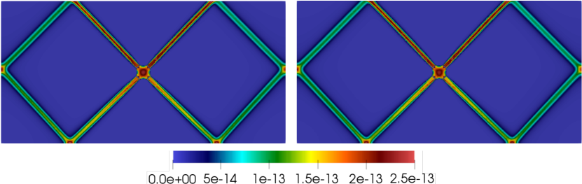
Figure 3: Second invariant of the strain rate pertaining to Example 2 using the composite formulation of a von Mises rheology with constant yield stress $\tau_{y}$ (left) and with depth-dependent yield stress (right). The depth-dependent yield stress is as specified in Figure 2.

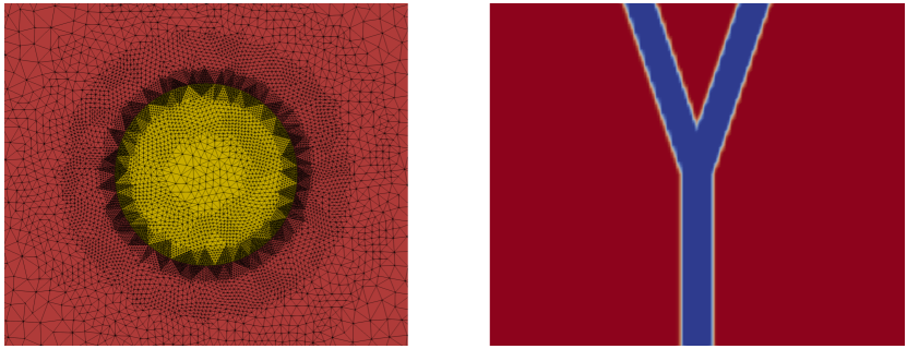
Figure 4: Viscosities of Examples 2 and 3. Left: Zoom-in of the locally refined mesh around the circular inclusion with radius 0.1 km in Example 2. The viscosity outside the the inclusion (in red) is several orders of magnitude larger than inside (in yellow). Right: Top view of the viscosity of the Y-shaped notch (in blue) of the 3-dimensional Example 3. Shown is a cutout of size $1\times 1$. The angle between the two branches of the notch is $2\tan^{-1}(1/3)\approx 37^{\circ}$.

Example 3: 3D compressional notch problem The third test problem is a three-dimensional variant of Example 1. The domain is a $120\text{ km}\times 60\text{ km}\times 30\text{ km}$ rectangular box, which has a viscoplastic upper layer with reference viscosity $\mu_{1}$ and yield stress $\tau_{y}$ and an isoviscous lower layer with constant viscosity $\mu_{2}$. Generalizing the setup from [33] used in Example 1, we introduce in the upper layer a Y-shaped notch (see the top view in Figure 4, right) with constant viscosity $\mu_{2}$. At the left and right sides, we enforce inflow boundary conditions, ${\boldsymbol{u}}\cdot{\boldsymbol{n}}=-u_{0}$, and at the fore, aft, and bottom boundaries we use ${\boldsymbol{u}}\cdot{\boldsymbol{n}}=0$ Dirichlet boundary conditions. At the top and for tangential velocities we apply homogeneous Neumann boundary conditions. With this test problem, we study the behavior of our algorithms for three-dimensional problems, their scalability, and their behavior when used in combination with adaptive mesh refinement of nonconforming hexahedral meshes. The parameters are the same as in Example 1, namely, $u_{0}=2.5~{}\text{mm/yr}$, $\mu_{1}=10^{24}~{}\text{Pa}\>\text{s}$, $\mu_{2}=10^{21}~{}\text{Pa}\>\text{s}$, $\underline{\mu}=10^{19}~{}\text{Pa}\>\text{s}$, and $\tau_{y}=10^{8}~{}\text{Pa}$. Note that in this example, the edges/faces of mesh elements are not aligned parallel to the boundary of the notch as they were in the examples before. Instead, we use a smooth transition from the reference viscosity $\mu_{1}$ of the upper layer to the viscosity $\mu_{2}$ of the notch and lower layer. This is carried out by first calculating the (shortest) distance $d$ between a mesh point and the interface and assigning the reference viscosity of the upper layer to be $\mu_{2}+(\mu_{1}-\mu_{2})\exp^{-1000d^{2}}$. This rapidly varying but smooth reference viscosity allows us to represent the physics of the Stokes problem with a sufficiently refined mesh. Moreover, along with solving the nonlinear equations, we adaptively refine the mesh in between Newton iterations and thus resolve viscosity gradients that are introduced through the nonlinear rheology.

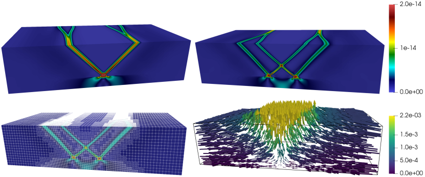
Figure 5: Flow pertaining to Example 3 with ideal viscoplasticity rheology. The top row shows the second invariant of the strain rate in front view (top left) and back view (top right). The bottom row shows the corresponding adaptively refined mesh (bottom left) and the velocity field (bottom right) with arrows colored by the velocity in $z$-direction.

Discretization and implementation details We now briefly summarize the discretization and implementation we use for our computational results. While the development of efficient and scalable solvers and preconditioners for (linearized) Stokes problems is an interesting and active field of research, here we focus on the behavior of the nonlinear iterations and give only a brief summary of the computational methods used. We discretize the Stokes equations using stable finite element pairings for the velocity and pressure variables. Note that one could use different (stable or stabilized) finite element pairings from those used here, or even different discretization methods such as staggered finite differences [4].

For the two-dimensional problems, unless stated otherwise, we use standard $P_{2}\times P_{1}$ Taylor-Hood elements on triangular meshes [7] and discontinuous linear elements for the stress variable. We also report results with higher-order Taylor Hood elements. Additionally, we experimented with stable element pairings with discontinuous pressure spaces. Since we observed very similar convergence behavior, we decided to not show these results. Our two-dimensional implementation is based on the open source finite element library FEniCS [19] and thus uses weak forms and numerical quadrature to compute finite element matrices. We found it beneficial to the convergence of iterative methods (in particular, Newton-type methods) to increase the numerical quadrature order, for example to 10. Doing so results in small quadrature errors and thus accurately approximated weak forms. These are important when linearization is done on the weak form level (as in FEniCS), to avoid having linearization and quadrature interfere and small numerical errors spoil the fast local convergence of Newton-type methods. Even with lower quadrature, however, we find good convergence but usually observe suboptimal convergence close to the solution. The linear problems arising in each Newton step are solved with a direct solver. To compute an appropriate step length for the Newton updates, we check whether the optimization objective in (6) decreases, and we reduce the step length if this is not the case. We compared using the optimization objective with using the nonlinear residual in this step length criterion and found that the two methods behave similarly.

For the three-dimensional problem, we use $\mathbb{Q}_{2}\times P_{1}^{\text{disc}}$ elements on nonconforming hexahedral meshes [7, 30]. The dual stress variable is treated pointwise at quadrature nodes and not approximated by using finite elements. This implementation builds on our previously developed scalable parallel software framework [30, 29]. To solve the (large) linear systems that arise, we use an iterative Krylov method with a block preconditioner for the Stokes system, which entails a Schur complement preconditioner. The viscous block in the Stokes system and components in our Schur complement preconditioner are amenable to multigrid methods. Hence, we have developed a hybrid (geometric and algebraic) multigrid method for adaptive meshes [30, 29]. For these three-dimensional problems, the step length for the Newton update is found by checking descent in the $L^{2}$-norm of the nonlinear residual, which amounts to approximately inverting a mass matrix during the inner product: $\left\lVert\boldsymbol{r}\right\rVert_{L^{2}}=\left\lVert\mathbf{r}\right\rVert_{\mathbf{M}^{-1}}=\sqrt{\mathbf{r}^{\mathsf{T}}\mathbf{M}^{-1}\mathbf{r}}$, for a residual vector $\mathbf{r}$ and the mass matrix $\mathbf{M}$ of the corresponding finite element space. In practice, it is beneficial for time to solution to employ an inexact Newton–Krylov method: far from the nonlinear solution, the stopping tolerance of the Krylov linear solver is set to a relatively high value, whereas closer to the nonlinear solution, the tolerance is decreased. Since this paper focuses on Newton’s method, we set a low Krylov tolerance $<10^{-7}$ throughout the nonlinear solve in our numerical examples.

The next section discusses qualitative properties of the solutions to the test problems and compares the convergence of the algorithms from Section 4.

6 Numerical Results

In this section, we study the performance of our algorithms for the two- and three-dimensional test problems described above. We also study the differences in the solutions resulting from using the ideal and the composite viscoplastic rheology laws, and we numerically verify the energy minimization properties of Stokes solutions derived in the preceding sections.

6.1 Comparison between ideal and composite plasticity

First, we compare the solution structure obtained with (2a) and (2b), the ideal and the composite von Mises rheology laws, respectively. Figures 6 and 7 show the second invariants of the strain rates for Example 1 when solved by using these two variants of combining the yield and reference viscosities. As illustrated in Figure 1 and as discussed previously in in Appendix C in [33], the composite rheology law can be considered as a regularization of the ideal plasticity due to a smooth transition between yielding and reference viscosity. Since the composite viscosity is always below the ideal viscosity, it leads to smaller strain rates in the solutions, as demonstrated in Figures 6 and 7. This difference in magnitude appears to be stronger for the problem with depth-dependent von Mises rheology (Figure 7). Additionally, the shape of the fault zone differs slightly, in particular close to the notch; and the second invariant of the strain rate is smoother for the composite rheology. This is, again, likely a consequence of the smooth way the yield viscosity is combined with the reference viscosity in the composite rheology law. This comparison shows that the definition of the viscoplastic rheology may impact the magnitude and potentially the structure of the solution; thus the two models cannot be interchanged.

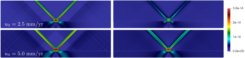
Figure 6: Comparison between ideal (left column) and composite rheology (right column) for von Mises rheology with constant yield stress and for two different values of lateral inflow velocities $u_{0}$. Colors depict the second invariant of the strain rate for Example 1.

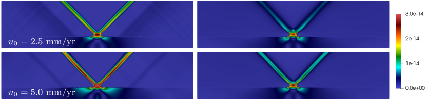
Figure 7: Comparison between ideal (left column) and composite rheology (right column) for depth-dependent von Mises rheology and for two different values of lateral inflow velocities $u_{0}$. The values for the depth-dependent yield stress are as specified in Figure 2. Colors depict the second invariant of the strain rate for Example 1.

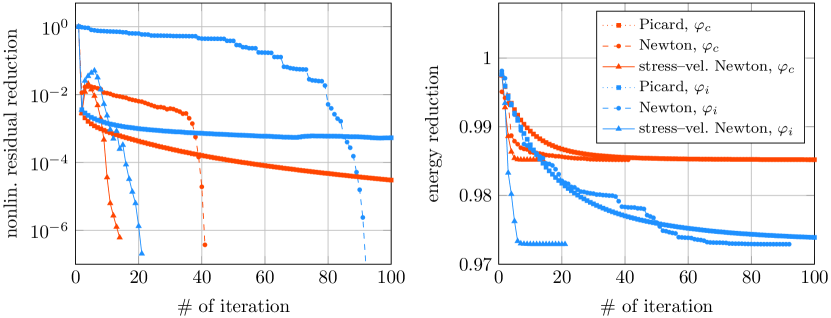
Figure 8: Convergence behavior of Example 1 for different iterative methods and ideal (blue curves) and composite (red curves) viscoplasticity. Shown on the left is the nonlinear residual reduction in each iteration and on the right the corresponding reduction of the energy objective (6).

6.2 Results for the three-dimensional problem

Numerical solutions for Example 3, a three-dimensional version of the notch problem, are shown in Figure 5. The symmetric V-shaped faults from Example 1 split into thinner W-shaped faults due to the shape of the notch along the interface of the upper and lower layers (see Figure 4, right). Figure 5, bottom right shows the velocity field (green arrows) at the nonlinear solution, where the central region is uniformly lifted with two lateral secondary uplift regions due to the secondary faults caused by the geometry of the notch.

We performed the three-dimensional computations on two uniformly refined meshes, including a relatively coarse mesh, which sufficiently resolves physical features, of 262,144 elements and a fine mesh of 2,097,152 elements, which is generated by one additional level of refinement. Further, we performed nonlinear solves with adaptive mesh refinement in between Newton iterations. The mesh adaptation starts from a uniform mesh of 262,144 elements and coarsens and refines based on the average second invariant of the strain rate per element: $\frac{1}{|\Omega_{e}|}\int_{\Omega_{e}}\dot{\varepsilon}_{\textsc{ii}}^{{\boldsymbol{u}}}({\boldsymbol{x}})d{\boldsymbol{x}}$, where $|\Omega_{e}|$ is the volume of an element $e$. The adaptation is triggered after a Newton step until the fifth nonlinear iteration, if it is needed. The final adapted meshes have a maximum refinement that is one level finer than the fine uniform mesh mentioned before. They differ in size for standard and stress–velocity Newton due to differences in the convergence of the solvers, having 881,945 and 1,107,758 elements, respectively. One example of an adapted mesh is depicted by the white edges in Figure 5, bottom left.

6.3 Nonlinear solver convergence

Next we study the convergence behavior of the different nonlinear iterative methods. Figures 8, 9, and 10 show the convergence history for Examples 1, 2, and 3. First, we observe that all algorithms converge faster for the composite compared with the ideal rheology (red vs. blue curves in Figure 8). This result is likely due to the higher regularity of the composite rheology (2b) compared with the ideal rheology (2a), which involves the pointwise $\min$-function. As is well documented in the literature, the Picard fixed-point method initially reduces the nonlinear residual rapidly but makes very slow progress in later iterations (see Figure 8), in particular for the highly nonlinear ideal rheology. The standard Newton method makes very slow progress initially until it reaches the “basin” of fast convergence, where it performs with the expected fast convergence. Furthermore the figure demonstrates that the stress–velocity Newton method converges rapidly for both types of viscoplastic laws (a factor of 2.5–5 fewer iterations than standard Newton), which is one of the key advantages of these novel nonlinear solvers. Note that the numerical results support the theoretical observation at the end of Section 4.2 that, if the stress variable is initialized with zero, the first iteration of stress–velocity Newton coincides with the first iteration of the Picard method.

The main reason for the vastly different behavior between the standard Newton and the stress–velocity Newton method can be seen in the step length plot of Figures 9, right. The line search reduces the length of standard Newton steps drastically in most iterations except the the very end, while the stress–velocity Newton method mostly makes full steps of length 1. A heuristic explanation for this behavior is that by introducing the additional stress variable into the nonlinear Stokes problem and using the transformation (14), the system becomes “less” nonlinear.

The results for Example 1 also show that while the nonlinear residual is not reduced monotonically, the energy objective (6) decreases monotonically (Figure 8, right). Since the objective is used to check descent when using the Newton update, this shows that using the objective from the underlying optimization problem for descent might be superior to using the nonlinear residual because it allows larger steps.

Our observations of the two-dimensional examples carry over to the three-dimensional example in Figure 10. The top graph of this figure shows the nonlinear convergence using the computationally more challenging ideal viscoplastic rheology. We have performed numerical experiments on three mesh configurations with increasing resolution comprised of a relatively coarse uniform mesh (Unif-C), a fine uniform mesh (Unif-F), and adaptively refined meshes (see Section 6.2 for more details). The finest mesh is achieved with the adaptively refined setup. It has an additional level of refinement to (Unif-F) that is assumed only locally resulting in fewer mesh elements overall than with uniform refinement. The (Unif-C) mesh consists of 262K elements, the (Unif-F) mesh with one additional level of refinement has 2.1M elements, and the (AMR) meshes have $\sim$1M elements. The stress–velocity Newton method takes about 20 iterations to reduce the nonlinear residual by 8–10 orders of magnitude for all three mesh configurations. The corresponding step lengths of stress–velocity Newton reduce below one only during the initial eight iterations (i.e., far from the solution) due to backtracking line search, but they remain at one until the algorithm has converged. The convergence of standard Newton is slower by a factor of four for the (Unif-C) mesh and increases to a factor of nine for the (AMR) setup, which has the highest level of local mesh refinement. Simultaneously with stagnating convergence, we observe a dramatic reduction of step lengths until a somewhat random inflection point when the desired super-linear Newton convergence reduces the residual quickly.

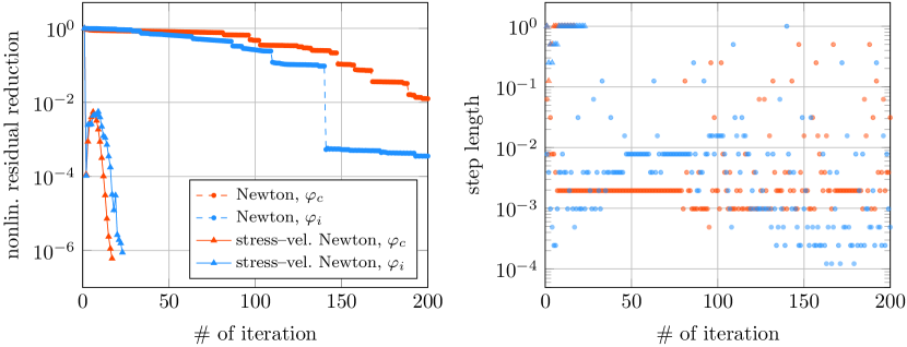
Figure 9: Convergence behavior for Example 2. Shown on the left is the residual reduction for standard and stress–velocity Newton for ideal (blue curves) and composite (red curves) rheologies. For ideal viscoplasticity, the lower viscosity bound $\underline{\mu}$ is important for convergence of the standard Newton method. If it is reduced by a factor of 10, the line search fails after 65 iterations (the stress–velocity Newton method still converges). The right plot shows the update step sizes these methods take.

Table 3: Convergence with varying mesh size for the composite rheology of Example 2. We list the number of iterations to reduce the nonlinear residual by $10^{-6}$.

# mesh elements	2,140	7,416	24,617	91,350
# standard Newton iterations	53	104	287	400
# stress–vel. Newton iterations	18	119	219	417

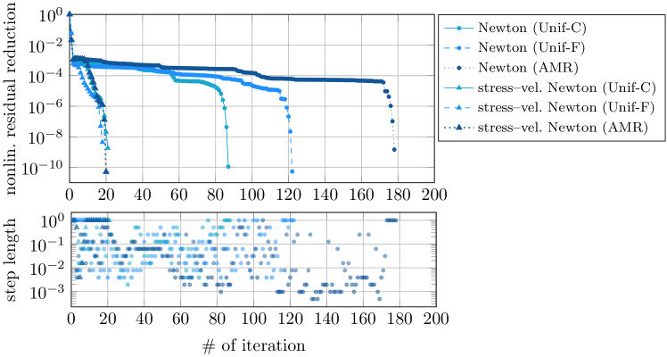
Figure 10: Convergence results for the three-dimensional Example 3 using the ideal viscoplastic rheology $\varphi_{i}$. The coarse uniform mesh (Unif-C) consists of 262K elements, the fine uniform mesh (Unif-F) with one additional level of refinement has 2.1M elements, and the final adapted meshes (AMR) with another additional level of max refinement have $\sim$1M elements. We observe a mesh-independent convergence of stress–vel. Newton. It is also faster than standard Newton by a factor of 4–9, where convergence deteriorates with finer mesh resolutions.

6.4 Solver behavior under mesh refinement and increasing order

In particular for solving large-scale problems, it is crucial that iterations numbers are insensitive to the refinement of the mesh and also the polynomial degree. Thus, in Table 3 we study the behavior of the standard and stress–velocity Newton method for meshes with an increasing number of elements. As can be seen, the iteration number for the standard Newton method grows significantly, while the iteration number for the velocity–stress Newton method remains constant. A similar test, now for increasing the order of the discretizations while keeping the mesh fixed, is shown on the right of Figure 11. We find that the convergence behavior for the stress–velocity Newton method does not change significantly when the polynomial order for the velocity discretization is increased from order $k=2$ to $k=5$, while the number of iterations increases with the polynomial order for the standard Newton method.

Supporting our results for two-dimensional problems using the FEniCS library, our code for three-dimensional problems shows similar convergence properties with respect to mesh refinement in Figure 10. It shows three mesh configurations with increasing level of refinement, where (Unif-C) and (Unif-F) are coarse and fine uniform meshes, respectively, and (AMR) has one additional level of local adaptive refinement compared to (Unif-F) (see Sections 6.2 and 6.3 for more details). Stress–velocity Newton requires only about 20 iterations until convergence and remains independent of mesh size. In contrast, the iteration counts of standard Newton depend heavily on the mesh resolution and increase by factor of $\sim$1.5 each time the mesh gains an additional level of refinement: taking 87, 122, and 178 iterations for (Unif-C), (Unif-F), and (AMR) meshes, respectively. These numerical results demonstrate the significant advantages of the stress–velocity Newton method for large-scale three-dimensional viscoplastic problems.

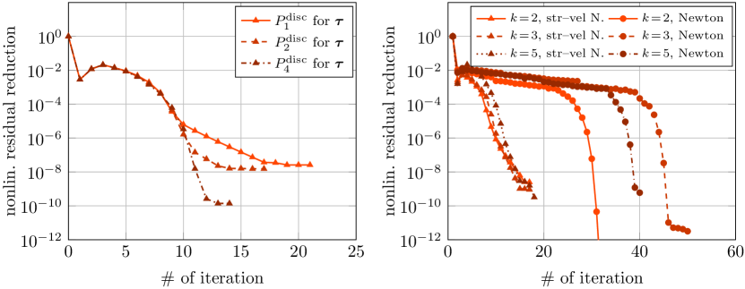
Figure 11: Tests with higher-order discretizations for Example 1 with composite rheology and parameters as detailed in Figure 8. Shown on the left is the residual reduction using standard Taylor-Hood elements, namely, order $k=2$ for the velocity and $k-1$ for the pressure, but with different-order discontinuous elements to discretize the stress tensor $\boldsymbol{\tau}$. Shown on the right is the behavior of the standard and the stress–velocity Newton methods for higher-order Taylor-Hood discretizations, namely, order $k$ for velocity and order $k-1$ for the pressure. The stress tensor is always discretized with polynomials of degree $k-1$. These runs use a coarser mesh consisting of 1,892 elements.

7 Conclusions

While viscoplastic rheologies are important for numerical models of the lithosphere, the resulting nonlinearity in the equations has been challenging for computational solutions. For viscoplastic rheologies where the yield stress does not depend on the dynamic pressure, we propose a novel Newton-type method in which we formally introduce an independent stress variable, compute the Newton linearization, and then use a Schur complement argument to eliminate the update for the stress variable from the Newton system. Hence, our method requires solving a sequence of linear Stokes problems that have the usual velocity–pressure unknowns. This method mostly allows one to take full unit length Newton update steps and thus converges significantly faster than the standard Newton method and the Picard method; and it is at least as fast as combined Picard–Newton methods, which require manual tuning and do not generalize well to different problem setups. We also observe that the number of iterations the method requires is independent of how fine the discretization is and which polynomial order is used to approximate velocity and pressure.

We also compare two von Mises rheology formulations: an ideal variant that uses a pointwise $\min$-function and a composite variant that uses the harmonic mean and, therefore, has effective viscosities that always lie below the ideal variant. While the two variants are sometimes used interchangeably, we find that they lead to solutions of rather different magnitude. Because of the improved smoothness, all solution algorithms in our comparison converge faster for the composite than for the ideal rheology. Furthermore, we study the uniqueness of solutions pertaining to the two rheologies using variational energy minimization arguments. We find that problems with the composite rheology always have a unique solution, whereas problems with ideal von Mises viscoplasticity require a regularization to ensure that they have a unique solution. In Example 2, we find that this regularization parameter can also play a practical role for the convergence of the standard Newton algorithm; see Figure 9.

Systematic study is needed to determine whether the novel methods can be extended to obtaining better converged solutions for rheologies with generalizations of the von Mises viscoplasticity, such as viscoelastoplasticity and rheologies where the yield stress depends on the dynamic pressure, also referred to as Drucker–Prager.

Government License The submitted manuscript has been created by UChicago Argonne, LLC, Operator of Argonne National Laboratory (“Argonne”). Argonne, a U.S. Department of Energy Office of Science laboratory, is operated under Contract No. DE-AC02-06CH11357. The U.S. Government retains for itself, and others acting on its behalf, a paid-up nonexclusive, irrevocable worldwide license in said article to reproduce, prepare derivative works, distribute copies to the public, and perform publicly and display publicly, by or on behalf of the Government. The Department of Energy will provide public access to these results of federally sponsored research in accordance with the DOE Public Access Plan.
https://energy.gov/downloads/doe-public-access-plan

References

- [1] Franco Brezzi and Michel Fortin. Mixed and hybrid finite element methods, volume 15 of Springer Series in Computational Mathematics. Springer-Verlag, New York, 1991.
- [2] James D Byerlee. Brittle-ductile transition in rocks. Journal of Geophysical Research, 73(14):4741–4750, 1968.
- [3] Tony F. Chan, Gene H. Golub, and Pep Mulet. A nonlinear primal-dual method for total variation-based image restoration. SIAM Journal on Scientific Computing, 20(6):1964–1977, 1999.
- [4] M Dabrowski, M Krotkiewski, and DW Schmid. MILAMIN: MATLAB-based finite element method solver for large problems. Geochemistry, Geophysics, Geosystems, 9(4), 2008.
- [5] Juan De los Reyes and Sergio Gonzalez Andrade. Path following methods for steady laminar Bingham flow in cylindrical pipes. ESAIM Mathematical Modelling and Numerical Analysis, 43:81–117, 01 2009.
- [6] Thibault Duretz, Alban Souche, Rena de Borst, and Laetitia Le Pourhiet. The benefits of using a consistent tangent operator for viscoelastoplastic computations in geodynamics. Geochemistry, Geophysics, Geosystems, 19(12):4904–4924, 2018.
- [7] Howard C. Elman, David J. Silvester, and Andrew J. Wathen. Finite elements and fast iterative solvers: with applications in incompressible fluid dynamics. Numerical Mathematics and Scientific Computation. Oxford University Press, Oxford, second edition, 2014.
- [8] Haakon Fossen. Structural Geology. Cambridge University Press, 2016.
- [9] M R T Fraters, W Bangerth, C Thieulot, A C Glerum, and W Spakman. Efficient and practical Newton solvers for non-linear Stokes systems in geodynamic problems. Geophysical Journal International, 218(2):873–894, 04 2019.
- [10] Philippe Fullsack. An arbitrary Lagrangian-Eulerian formulation for creeping flows and its application in tectonic models. Geophysical Journal International, 120(1):1–23, 1995.
- [11] A. Glerum, C. Thieulot, M. Fraters, C. Blom, and W. Spakman. Nonlinear viscoplasticity in ASPECT: benchmarking and applications to subduction. Solid Earth, 9(2):267–294, 2018.
- [12] Corinna Hager and B.I. Wohlmuth. Nonlinear complementarity functions for plasticity problems with frictional contact. Computer Methods in Applied Mechanics and Engineering, 198(41):3411 – 3427, 2009.
- [13] Michael Hintermüller and Georg Stadler. An infeasible primal-dual algorithm for total variation-based inf-convolution-type image restoration. SIAM Journal on Scientific Computing, 28(1):1–23, 2006.
- [14] S. Hüeber, G. Stadler, and B. I. Wohlmuth. A primal-dual active set algorithm for three-dimensional contact problems with Coulomb friction. SIAM Journal on Scientific Computing, 30(2):572–596, 2008.
- [15] Kolumban Hutter. Theoretical Glaciology. Mathematical Approaches to Geophysics. D. Reidel Publishing Company, 1983.
- [16] Tobin Isaac, Georg Stadler, and Omar Ghattas. Solution of nonlinear Stokes equations discretized by high-order finite elements on nonconforming and anisotropic meshes, with application to ice sheet dynamics. SIAM Journal on Scientific Computing, 37(6):B804–B833, 2015.
- [17] Boris J.P. Kaus. Factors that control the angle of shear bands in geodynamic numerical models of brittle deformation. Tectonophysics, 484(1):36 – 47, 2010. Quantitative modelling of geological processes.
- [18] Luc L. Lavier, W. Roger Buck, and Alexei N. B. Poliakov. Factors controlling normal fault offset in an ideal brittle layer. Journal of Geophysical Research: Solid Earth, 105(B10):23431–23442, 2000.
- [19] Anders Logg, Kent-Andre Mardal, and Garth Wells. Automated Solution of Differential Equations by the Finite Element Method: The FEniCS book, volume 84. Springer Science & Business Media, 2012.
- [20] Xiaolin Mao, Michael Gurnis, and Dave A May. Subduction initiation with vertical lithospheric heterogeneities and new fault formation. Geophysical Research Letters, 44(22):11,349–11,356, 2017.
- [21] Dave A May, Jed Brown, and Laetitia Le Pourhiet. A scalable, matrix-free multigrid preconditioner for finite element discretizations of heterogeneous Stokes flow. Computer Methods in Applied Mechanics and Engineering, 290:496 – 523, 2015.
- [22] Dave A. May and Louis Moresi. Preconditioned iterative methods for Stokes flow problems arising in computational geodynamics. Physics of the Earth and Planetary Interiors, 171:33–47, 2008.
- [23] C. Mehlmann and T. Richter. A modified global Newton solver for viscous-plastic sea ice models. Ocean Modelling, 116:96 – 107, 2017.
- [24] Louis Moresi and Viatcheslav Solomatov. Mantle convection with a brittle lithosphere: thoughts on the global tectonic styles of the Earth and Venus. Geophysical Journal International, 133(3):669–682, 1998.
- [25] John B. Naliboff, Magali I. Billen, Taras Gerya, and Jessie Saunders. Dynamics of outer-rise faulting in oceanic-continental subduction systems. Geochemistry, Geophysics, Geosystems, 14(7):2310–2327, 2013.
- [26] AA Popov and Stephan V Sobolev. SLIM3D: A tool for three-dimensional thermomechanical modeling of lithospheric deformation with elasto-visco-plastic rheology. Physics of the earth and planetary interiors, 171(1-4):55–75, 2008.
- [27] G. Ranalli. Rheology of the Earth. Springer, 1995.
- [28] Johann Rudi. Global convection in Earth’s mantle: Advanced numerical methods and extreme-scale simulations. PhD thesis, The University of Texas at Austin, 2018.
- [29] Johann Rudi, A. Cristiano I. Malossi, Tobin Isaac, Georg Stadler, Michael Gurnis, Peter W. J. Staar, Yves Ineichen, Costas Bekas, Alessandro Curioni, and Omar Ghattas. An extreme-scale implicit solver for complex PDEs: Highly heterogeneous flow in earth’s mantle. In SC15: Proceedings of the International Conference for High Performance Computing, Networking, Storage and Analysis, pages 5:1–5:12. ACM, 2015.
- [30] Johann Rudi, Georg Stadler, and Omar Ghattas. Weighted BFBT preconditioner for Stokes flow problems with highly heterogeneous viscosity. SIAM Journal on Scientific Computing, 39(5):S272–S297, 2017.
- [31] W Sharples, L-N Moresi, MA Jadamec, and Jerico Revote. Styles of rifting and fault spacing in numerical models of crustal extension. Journal of Geophysical Research: Solid Earth, 120(6):4379–4404, 2015.
- [32] S.V. Sobolev, A. Petrunin, Z. Garfunkel, and A.Y. Babeyko. Thermo-mechanical model of the Dead Sea Transform. Earth and Planetary Science Letters, 238(1):78–95, 2005.
- [33] Marc Spiegelman, Dave A May, and Cian R Wilson. On the solvability of incompressible Stokes with viscoplastic rheologies in geodynamics. Geochemistry, Geophysics, Geosystems, 17(6):2213–2238, 2016.
- [34] Paul J. Tackley. Self-consistent generation of tectonic plates in time-dependent, three-dimensional mantle convection simulations. Geochemistry, Geophysics, Geosystems, 1(8), 2000.
- [35] Donald L. Turcotte and Gerald Schubert. Geodynamics. Cambridge University Press, 2nd edition, 2002.
- [36] Richard von Mises. Mechanik der festen Körper im plastisch-deformablen Zustand. Nachrichten von der Gesellschaft der Wissenschaften zu Göttingen, Mathematisch-Physikalische Klasse, 1913:582–592, 1913.