Cloud Identification from All-sky Camera Data with Machine Learning

Abstract

Most ground-based observatories are equipped with wide-angle all-sky cameras to monitor the night sky conditions. Such camera systems can be used to provide early warning of incoming clouds that can pose a danger to the telescope equipment through precipitation, as well as for sky quality monitoring. We investigate the use of different machine learning approaches for automating the identification of mostly opaque clouds in all-sky camera data as a cloud warning system. In a deep-learning approach, we train a Residual Neural Network (ResNet) on pre-labeled camera images. Our second approach extracts relevant and localized image features from camera images and uses these data to train a gradient-boosted tree-based model (lightGBM). We train both model approaches on a set of roughly 2,000 images taken by the all-sky camera located at Lowell Observatory’s Discovery Channel Telescope, in which the presence of clouds has been labeled manually. The ResNet approach reaches an accuracy of 85% in detecting clouds in a given region of an image, but requires a significant amount of computing resources. Our lightGBM approach achieves an accuracy of 95% with a training sample of ${\sim}$1,000 images and rather modest computing resources. Based on different performance metrics, we recommend the latter feature-based approach for automated cloud detection. Code that was built for this work is available online.

1 Introduction

Ground-based telescopes are exposed to and have to be protected from environmental influences. Precipitation and high relative humidity can cause significant damage to optical surfaces, the telescope structure, as well as telescope electronics. In order to protect telescopes from rain and snow, the most conservative policy is to close their enclosures as soon as the sky is clouded out.

All-sky cameras provide an efficient and inexpensive means to monitor cloud coverage at night. Such cameras, which often use inexpensive charge-coupled-device (CCD) or complementary metal–oxide–semiconductor (CMOS) detectors in combination with wide-angle lenses provide the sensivity and dynamic range that is necessary to identify cloud coverage even on a dark night. Most observatories – ranging from small aperture telescopes to the largest available telescopes – already have such camera systems installed and use them on a regular basis.

Typically, human telescope operators monitor all-sky camera feeds in real-time, allowing them to react to incoming clouds by closing the telescope enclosure on short time scales. While the task of identifying clouds against the sky background is mostly trivial for humans, this is a non-trivial task for a machine. Problems arise because of the variable appearances clouds can have during the night. Depending on illumination conditions from the Moon or the Sun, clouds can either appear brighter than the clear sky, or darker. Furthermore, at the low imaging resolutions provided by all-sky cameras even the clear sky itself contains bright and dark patches, depending on the density and brightness of stars in a given field, creating a source of confusion in cloud identification. Additional complications arise from static or variable effects from terrestrial illumination and the observatory’s local horizon. A simple classification scheme, for instance based on sky brightness, is in most cases not sufficient to identify clouds with high confidence.

While the main motivation for this work is the development of a system that provides warning in the presence of opaque clouds that can potentially carry precipitation, the same methodology can be applied to quantify sky quality. Such a system can be used to derive the fraction of the accessible sky that is clear throughout a night or longer periods, or to identify near-photometric conditions without human interaction.

The automation of cloud discovery from all-sky camera data is worthwhile due to the ubiquity and general availability of these camera systems. An automated system that is able to warn a robotic telescope – or a human operator – of incoming clouds will significantly improve the safety of observatories and enable automated monitoring of sky quality.

In this work, we investigate the use of machine learning methods to identify and locate clouds in all-sky camera data using two different approaches. In our first approach, we use a deep-learning approach based on a residual neural network (ResNet) model that works on image data as obtained from the camera. Our second approach combines the extraction of carefully designed features that are indicative of clouds from images with a tree-based machine learning model (lightGBM).

Our requirement is to reach an accuracy of 95% for the identification of clouds for a given location on the sky from all-sky camera image data.

We define our models in Section 3, present their results in Section 4, and discuss their performances and possible application to different use cases in Section 5. Appendix A briefly discusses the implementation of the models and the code used in this work.

2 All-sky Camera Data

We train and test our machine learning models on image data taken at Lowell Observatory’s Discovery Channel Telescope. The images have been obtained with a Starlight Xpress Oculus all-sky camera, featuring a 1392$\times$1040 pixel CCD detector and a 1.55 mm f/1.2 fish-eye lens with a field of view of 180°. The camera creates a circular projection of the sky plane with a radius of 520 pixels and 16-bit dynamic range. Image files are provided in FITS format; the image header includes information on the date and time of the observation and the exposure time (typically 60 s at night). The imaging cadence at night is 1 min^-1. Figure 1 (panel a) shows a raw example image from this camera.

Figure 1: Preparation stages for our image data. (a) Raw image showing the circular projection of the sky and illumination on lens assembly parts. Clouds appear bright due to the imminent rise of the Moon; the Milkyway is visible, too. (b) Cropped image in which non-relevant parts for our task have been masked (telescope enclosure, nearby trees, and lens assembly). (c) Subregion grid resulting in 33 subregions. (d) Labeled subregion grid (subregions that contain significant amounts of clouds are highlighted).

2.1 Data Preparation

From each image we crop a quadratic region that contains the circular image of the sky.

We mask those parts of the image that do not show the sky – including parts of the lens assembly, as well as local background features like the telescope enclosure and trees – by settting the corresponding pixel values to zero. The mask is created from a median combination of 50 random images that were taken under similar (bright) illumination conditions. We blur the resulting combined image with a Gaussian filter (scipy.ndimage.filters.gaussian_filter) to remove small-scale features and use a threshold to extract those parts of the image that do not show the sky. Finally, we smooth the edges of our selection by convolving the resulting mask with a square kernel. The resulting mask has been applied in Figure 1 (panel b). While this approach does not perfectly mask all objects on the local horizon, it is sufficient for our purposes.

To roughly localize clouds in the image data, we divide each image into a set of subregions. The borders of these subregions are defined in terms of radial distance from Zenith and azimuth. The innermost subregion is a circular aperture centered on Zenith; more distant areas are arranged in rings that are sub-divided into equidistant ring-segments based on azimuth. This radially symmetric definition has the advantage that ring segments on the same ring correspond to the same elevation and the same airmass. Furthermore, this definition naturally reflects the ranked importance of finding clouds at different elevations: while clouds close to Zenith may pose an immediate threat to the observatory, clouds on the horizons are no immediate threat but should be recognized and monitored. This ranking can be directly translated into different warning levels.

For our data, we chose a scheme that consists of a circular aperture around Zenith, 3 rings, and 8 ring-segments. The distribution of the 33 resulting subregions is shown in Figure 1 (panel c).

2.2 Training Data Sample

Our training data sample consists of 1,975 images that were randomly drawn from a set of 259,259 images taken between June 2018 and August 2019. For each image we manually label the presence of clouds in each subregion with a binary flag. Subregions are assigned unity value if they contain considerable amounts of clouds that significantly affect the transparency in the corresponding subregions (see Section 5.2.2 for a discussion), or zero otherwise; thick cirrus affecting transparency is considered as a cloud, while thin cirrus maybe not be considered as a cloud. Figure 1 (panel d) shows a labeled example image.

From our 1,975 training data images, we extract 65,175 labeled subregions, 28,872 (44.3%) of which contain clouds, 36,303 (55.7%) of which do not contain clouds. Hence, our training data sample has a slight class imbalance that favors clear sky conditions.

3 Machine Learning Model Definitions

We use two different approaches and two different machine learning models to learn and predict the presence of clouds in our image data: a residual neural network (ResNet) that works with image data, and a tree-based model (lightGBM) that works on a set of carefully designed features that we extract from each image and subregion.

3.1 Image-Based Approach (ResNet)

We use a residual neural network (ResNet, Kaimang et al., 2015) adaptation that works directly on the cropped and masked image data. ResNets are frequently used in computer vision applications, including object identification, localization, classfication, and image segmentation.

Mimicking the way in which biological neural networks (e.g., the human brain) work, artificial neural networks consist of several layers of ”neurons” that are connected with each other and react to external stimulation in the form of an input data vector. Each neuron is a mathematical function that uses a weighting scheme to calculate a scalar output value based on the weights, the input data vector, and a non-linear activation function. In simple feed-forward neural networks, each neuron is fully connected to all neurons in the previous layer and all neurons in the following layer; outputs of the previous layer serve as input for the current layer, while the output of the current layer serves as input for the following layer. By carefully designing a neural network and training it with ground-truth data, it can learn patterns and perform tasks like image classification. The learning process is an optimization process that adjusts the weights in each neuron such that the output of the model agrees with the ground-truth. See Russel et al. (2009) and Goodfellow et al. (2016) for a review of the details of neural networks.

ResNets have a more complex network architecture including a number of convolutional layers and the outputs of neurons do not only affect the neurons in the following layer, but also those in later layers. This principle enables the training of extremely deep networks (with many layers) and thus the learning of rather complex tasks. See Kaimang et al. (2015) for more details.

We use the ResNet-18 implementation provided by torchvision.models.resnet and modify it in such a way that the first convolutional layer of the model is expecting single-channel (i.e., monochrome) images as input (instead of 3-channel RGB data) and uses a $16\times 16$ pixel convolutional kernel. Furthermore, the model produces an output vector of length 33, representing the 33 subregions in the image. As loss function, we choose the Binary Cross Entropy with Logits Loss (pytorch.nn.BCEWithLogitsLoss), which combines calculating the binary cross entropy between the training features (image data) and the training labels (presence of clouds) with a Sigmoid layer for additional non-linear activation. As optimizer we use Stochastic Gradient Descent with momentum (Goodfellow et al., 2016).

3.1.1 Training Procedure

We train our model in single-batch mode using 70% of the available training data (the remaining 30% are used as validation data sample) and start the optimization procress with a learning rate of 0.025, which decreases at a rate of 0.3 every 5th epoch for 100 epochs.

The training is performed on a standard desktop computer that is equipped with a NVIDIA GeForce GTX 1050 Ti graphics card, thus taking advantage of Pytorch’s GPU support.

The results of the training are presented in Section 4.1.

3.2 Feature-Based Approach (lightGBM)

We also use a gradient-boosted tree-based model that works on a set of features (see Section 3.2.1) that we extract from our images. The term “tree” refers in this case to a decision tree, which is a simple non-parametric machine learning model that can be used for classification. A decision tree is a directional graph of binary questions based on the provided feature space. In the case of a classification task, each “branch” of the tree ends in a “leaf”, which defines a class assignment. See Russel et al. (2009) for a discussion of decision trees.

A gradient-boosted tree-based model means the combination of a large number of decision trees and an optimization rule that builds succint trees to optimize the performance of the entire ensemble. Gradient-boosted tree-based models are extremely flexible and powerful in classification problems in pre-defined feature spaces.

We use the lightGBM (Ke et al., 2017) model implementation in combination with the sklearn.pipeline infrastructure to train our model. We evaluate sample scores using the cross entropy between model outputs and training labels.

3.2.1 Feature Definitions

We base the design of the feature space in which our tree-based model will learn on human experience and mimick criteria that a human would use in identifying clouds:

• source density: the presence of stars precludes the presence of thick clouds, which implies that subregions with a high density of sources most likely represent a clear patch of sky. We measure the number of sources per subregion with the Python module SEP, which in turns makes use of Source Extractor (Bertin & Arnouts, 1996). Sources are identified based on a minimum number of pixel that are brighter than the background by a given threshold; tuning these parameters depends somewhat on the detector. The source count obtained using this method typically represents a lower limit, due to the usually rather limited imaging resolution of the all-sky camera. We derive the source density by dividing the number of sources per subregion by the total subregion pixel area.

• background properties: depending on the illumination conditions (presence of the Moon or the Sun) clouds generally appear as dark or bright patches against the clear sky. We hence derive the average brightness, median brightness, and brightness standard deviation across each subregion.

• time derivatives: clouds are rarely stationary; we take advantage of this property and form differences for each of the aforementioned features for each subregion. In order to be sensitive to both fast-moving and slow-moving clouds, we form subregion-based differences of each of the aforementioned properties between the property of the current image and that of images that were taken 3 min ago and 15 min ago.

The proper interpretation of these features requires some additional information, which we also add to the feature space:

• solar and lunar elevation, lunar phase: all three measures provide valuable information on the illumination circumstances and address the question whether the model should expect clouds to be darker or brighter than the clear sky.

• subregion identifier: integer identifier of the current subregion, indicating its location on the local sky.

In total, the feature space considered encompasses 16 different features for each subregion and image in the training data set. In the training and prediction process we treat each subregion of each image as an independent datapoint with an input vector of length 16 and a scalar target value.

3.2.2 Training and Hyperparameter Tuning

We split the available labeled data sample into a validation sample, containing 10% of the examples, and another sample that is used in a randomized cross-validation approach with 5 folds. We evaluate the mean training and test scores in a uniform fashion over a wide range in the most relevant model parameters: the number of estimators, learning rate, maximum depth of each estimator, number of leaves per tree, and the minimum number of examples to form a leaf. Regularization is achieved by sampling L1 and L2 regularization parameters $\alpha$ and $\lambda$ on a logarithmic scale. The results of the training are presented in Section 4.2.

4 Results

4.1 ResNet

The performance of the ResNet model is somewhat sensitive to the learning rate and momentum, but outcomes are very similar for learning rates of the order of (1–3)% and momentum values 0.7–0.9. However, we do find significant variations between independent training runs despite the use of manual random seeding, which we attribute to random scheduling during the GPU acceleration and the relatively small training sample size for this type of model. In the following, we report on the results of the best of five independent training runs.

Figure 2 shows that we find validation sample accuracies of the order of ${\sim}$80%, peaking around 87% for individual training epochs. After ${\sim}$20 epochs, the training sample loss becomes mostly stationary, meaning that the model does not improve. The test sample loss, however, is subject to significant variations, which we attribute to the relatively small sample size. Training of the ResNet model leads to rather high validation sample accuracies of the order of 85% after only ${\sim}$10 training epochs. We adopt this accuracy and number of epochs in our further analysis. We find f1-scores of the order of 0.88. The f1-score is defined as the harmonic mean of precision and recall and serves as a measure for the overall performance of a binary classifier, where 1 denotes a flawless classification and lower values denote flawed classification results.

Training our ResNet adaptation for 100 epochs takes 6.9 hr, 10 epochs of training takes accordingly 41 min.

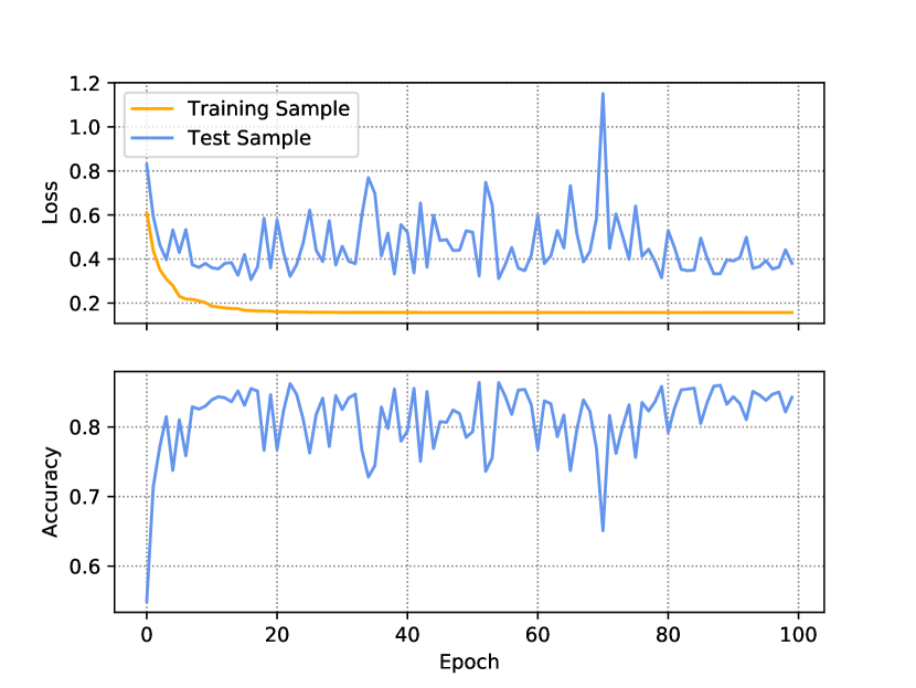
Figure 2: Loss (top) and test sample accuracy (bottom) of our ResNet model during 100 training epochs. After ${\sim}$20 epochs, the training sample loss is mostly stationary and the model barely improves. Given the low test sample loss and high test sample accuracy around 10 epochs, we recommend this number of epochs for training this model.

4.2 lightGBM

We adopt the following set of hyperparameters for our lightGBM model: a maximum depth of each tree of 5, 500 estimators, a learning rate of 0.25, 30 leaves per tree, 100 examples required to form a leaf, $\alpha=10$, and $\lambda=100$. This configuration leads to a training sample accuracy of 96% and a test sample accuracy of 95%. The accuracy on the validation sample, which was neither used in the training of the model nor in the tuning of the hyperparameters, is 95%, too. The f1-score on the validation sample is 0.94, underlining the good performance of the trained model.

The training of the entire training sample using the selected hyperparameters and a 5-fold cross-validation takes 12 s on a standard desktop computer.

Figure 3 shows the feature importances extracted from the final trained model. The feature importance used here is defined as the number of times a feature is used in this model throughout all individual decision trees. The comparison shows that environmental parameters that affect sky brightness are extremely important, followed by the subregion location. Actual subregion properties and their time differentials follow, the latter of which only have a small – but not negligible – impact on the model results.

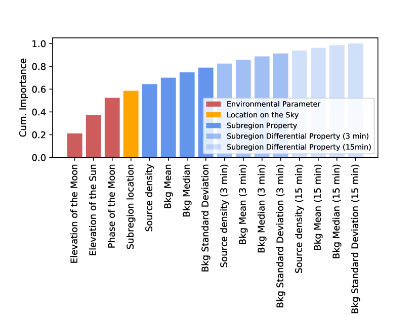
Figure 3: Cumulative feature importances extracted from the trained lightGBM model ordered by magnitude. Environmental parameters affecting the sky brightness play a major role in the identification of clouds, followed by the location in the sky. Subregion properties and their differentials play a decreasingly important role with time.

5 Discussion

5.1 Model Performance

We find the feature-based approach using lightGBM to be both significantly faster and more accurate than our image-based approach using the ResNet adaptation. Only our lightGBM approach meets our requirement of properly identifying 95% of subregions that contain clouds. This discrepancy can be explained with the fact that our feature-based approach takes advantage of pre-defined features guided by human experience which the ResNet model has to learn by itself.

While the feature-less approach using our ResNet model shows some promise, this model most likely requires much more training data to reach a similar accuracy as our lightGBM model. However, the need of more training data, which has to be labeled manually, in combination with the much higher computational requirements, make this deep learning approach much less attractive.

5.1.1 Model Accuracy and Confusion Matrix

The cloud detection probability for a single subregion is ${\sim}85$% using ResNet and ${\sim}$95% using lightGBM. Since clouds typically cover more than one subregion, the probability that any subregion in a set of $N$ subregions that actually include clouds increases exponentially with $N$. In the same way, the probability to miss clouds decreases. For example, the probability to miss the detection of clouds in three different subregions with the lightGBM classifier is ${\sim}0.05^{3}=10^{-4}$. Hence, the confidence in detecting the presence of clouds anywhere on the sky is much higher than the probability to detect them in a single subregion, supporting the usefulness of this machine-learning approach.

We further investigate the performance of our models using a confusion matrix, which not only provides information on the overall classification accuracy, but also additional information on the rate of false positive and false negative classifications. Here, a false positive classification means a subregion that has been predicted to contain clouds, although this is not the case. A false negative classification refers to a subregion that contains clouds which are not identified by the classifier. The confusion matrices for both methods used here are shown in Figure 4.

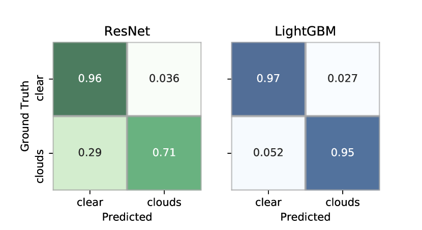
Figure 4: Confusion matrices for the methods considered in this work.

As Figure 4 shows, the false negative and false positive rates using the lightGBM classifier are rather small at 5.2% and 2.7%, respectively. We point out that the false negative rate is roughly a factor 2 higher than the false positive rate, which might be slightly affected by the class imbalance inherent to the training data sample (see Section 2.2), but is mostly likely due to the classifier’s inability to identify non-opaque clouds that were labeled in the training data set. This effect, as well as additional shortcomings potentially related to the insufficient size of the training sample (see Section 5.2.1), is much more obvious in the results of the ResNet classifier, which achieves a false negative rate of 29% and a false positive rate of 3.6%, underlining the insufficient performance of this classifier. The comparison of these numbers support the suitability of the lightGBM approach for this task, which is able to identify clouds with high confidence.

We note that for both model approaches the rate of misclassifications (false positives and false negatives) is highest for subregions close to the horizon. This is most likely due to confusion with layers of haze or other near-surface effects, as well as human subjectivity introduced in the training sample (see Section 5.2.2). This issue is most likely to be resolved with more consistent manual labeling of a larger training sample.

5.2 Training Data

The performance of each model depends highly on the amount and quality of the available training data sample.

5.2.1 How much training data is needed?

We investigate the impact of the training data sample size on the model performance by training the same models on random subsamples of the original training data sample. We use the same sets of hyperparameters presented in Section 4. Results for different subsample sizes are listed in Table 1.

Table 1: Model Performance as a Function of Training Sample Size.

Training Sample Size	ResNet		lightGBM
(Nimages)	Accuracy	F1	Accuracy	F1
1975	0.843	0.877	0.946	0.937
1000	0.816	0.847	0.945	0.939
500	0.762	0.795	0.932	0.919
100	0.552	0.591	0.915	0.910

In the case of our ResNet approach, a steady rise of both accuracy and F1-score can be observed through all training sample sizes used in this analysis. The fact that neither metric plateaus indicates that the trainig sample size required to max out the performance of the ResNet model has not been reached and that this model will benefit from additional training data. We fit a power-law function of the form $f(x;a,b,c)=a-b\cdot 10^{c}$ to the ResNet accuracy values in Table 1 and find a saturation accuracy of only 92%. Furthermore, we find through extrapolation that our ResNet approach requires of the order of 20,000 training samples to achieve an accuracy of 90%. We acknowledge that this extrapolation may not be highly accurate, but it certainly provides reasonable estimates of the orders of magnitudes for both the maximum accuracy that can be expected and the training sample size. Based on these estimates, we conclude that our ResNet approach in this form is extremely expensive compared to our lightGBM model.

We find lightGBM performances that are comparable to those reported in Section 4.2 for training sample sizes of the order of 1000 image examples. Even in the case of only 100 image examples, an accuracy above 90% can be reached. This result implies that the lightGBM approach is useful even if only a small training sample is available. We furthermore conclude that more then 1000 training examples will not significantly improve the performance of this model.

5.2.2 Training Data Quality and Cloud Definition

The training data sample should contain as little noise as possible in order to maximize the model performance. However, it is not always possible to provide unambiguous training data in the case of cloud identification, as it is a highly subjective process even for a human.

Clouds have many different ways to manifest in all-sky camera images, making it nearly impossible to come up with a clear definition what counts as a cloud and what not. Does thin cirrus count as a cloud? Do you consider a subregion to contain a cloud if it occupies less than 10% of that subregion’s area? Does haze on the horizon count as a cloud? There is no definitive answer to these questions, adding a significant amount of noise to the training data sample.

The sensitivity of any machine learning effort to cirrus and other not fully opaque clouds depends highly on the training data provided. Based on the goal set for this work – the implementation of a cloud warning system – we chose a rather conservative cloud definition in the sense that we expect a cloud to be fully opaque. While this definition is less prone to human subjectivity (leading to a more homogeneous training sample), it clearly creates a bias in the quantification of sky quality (e.g., cirrus is likely to be not detected as a cloud), which becomes apparent in the false negative rates of both classifiers (see Section 5.1.1). A less conservative cloud definition can lead to a better detectability of cirrus, but might be susceptible to other phenomena like air glow and terrestrial light sources. Additional processing of the input data might be necessary to distinguish the latter two effects from cirrus, e.g., by exploiting their static nature in the night sky. We leave such investigations for the future.

Both of our models utilize regularization mechanisms to be able to generalize the training data and to cope with noise in the training data. However, this also means that the subjective uncertainty of humans is propagated into the models: if the presence of clouds in a given subregion is vague to a human, it will also be vague to the model trained on data labeled by a human. Any labeling efforts by humans should thus be as consistent as possible.

We hence believe that the performance any model can achieve is mainly limited by the quality of the training data sample.

6 Conclusions

We find that the identification of clouds in all-sky camera data is a solvable task for machine learning models. We use two different approaches for this task: a ResNet model that works with image data and achieves an accuracy of ${\sim}85$%, and a lightGBM model that uses features extracted from the images and achieves an accuracy of ${\sim}$95%. While we find false negative and false positive rates of only a few percent for the lightGBM model, the ResNet model has a false positive rate of ${\sim}$3% and a false negative rate of 29%. These estimates are based on a training data sample containing 1975 images. While we expect a slightly better performance for the ResNet model wih a larger sample size, the lightGBM model seems to require only 1000 training samples to obtain its full performance.

In conclusion, we recommend the use of feature extraction in combination with a simple classification model, like lightGBM, as it provides superior performance in terms of accuracy and runtime.

The methods presented here are tailored to the detection of opaque clouds, i.e., for the protection of observatory equipment from weather. This is mostly achieved through the cloud definition that is applied in the labeling of the training data set. Additional steps will have to be taken to extend the usability of this methods for automated sky quality quantification that is also able to detect even thin cirrus or photometric conditions.

Appendix A Implementation and Resources

The code built for this work is publicly available under a 3-clause BSD-style license at https://github.com/mommermi/cloudynight (Mommert, 2020). The cloudynight repository contains (1) a Python module for data handling and preparation, feature extraction, model training and prediction, (2) a Python Django web server application for database management, data visualization, and manual labeling, (3) example data used in this work, and (4) a number of scripts for testing the functionality on the example data.

Please note that this code is not intended for plug-and-play. Instead, it is tailored to the example data used in this work. However, with the descriptions in this appendix and comments provided as part of the code, it should be easy to modify the code of the module and the web application to run them on other data sets.

The example data provided are sufficient to test the different parts of the provided code. However, especially the image data are not sufficient to train a meaningful model. Also note that due to the small number of images included in the example image set, it is impossible to derive time-dependent features from images – these features are hence set to zero in this case.

A.1 Design, Premises, and Setup

The cloudynight module consists of three classes: AllskyImage, which handles individual allsky images, AllskyCamera, which handles image management and provides wrapper methods for image sets, and LightGBMModel, which handles the lightGBM model used in this work. Note that the ResNet model implementation is provided as an example script, but not as part of cloudynight. A large fraction of the module’s setting are configurable using parameters defined by cloudynight.conf (in the file __init__.py).

Camera images are expected in FITS format. Each image should have a header containing at least the date and time of observation (header keyword DATE-OBS). Camera images are also expected to be sorted by night and to reside on a remote machine. The latest data for a given night can be downloaded from that remote machine with AllskyCamera.download_latest_data, which uses an rsync call to only copy new data; this mechanism requires the exchange of ssh keys between both machines. Downloaded images for a given night can be processed (prepared and feature-extracted) and results can be uploaded to the database with AllskyCamera.process_and_upload.

The database has to be setup as part of the Django web application. The use of array fields in the database requires a PostgreSQL database type. The setup of this web application is detailed in the repository documentation. The web application provides a RESTful API that can be used to access and modify the database from any other machine on the network, e.g., to run a trained model on a given image to detect clouds.

The database contains 3 tables:

• Subregion: contains outlines of the individual subregions for proper display in the web application;

• Unlabeled: contains image features for images that have not been labeled manually;

• Labeled: contains image features and cloud labels for images that have been labeled manually; this is the training data set.

Before using the web application, an image mask has to be created using the script generate_mask.py and the subregion outlines have to be uploaded to the database using the script subregions.py.

A.2 Training

After the proper setup of the module and the web application, training data have be generated. For this purpose, data from a large number of nights should be downloaded, processed, and uploaded to the Unlabeled table of the database using AllskyCamera.process_and_upload_data. The training task (label/) of the web application can now be used to manually label subregions that contain clouds; results are automatically saved to the Labeled table of the database.

A.3 Model Fitting

If enough training data are available, a model can be fitted The script model_lightgbm.py can be used as a template for this task. Model performances for different model parameters can be explored with LightGBMModel.train_randomizedsearchcv. Once a model solution has been found, the model has to be saved as a file using LightGBMModel.write_model so that the trained model can be utilized by the web application.

A.4 Cloud Detection

The presence of clouds can be predicted for the latest camera using the web application task predictLatestUnlabeled/. This task returns a json object that contains an array in which each element represents one subregion; the value of the element will be 1 in case a cloud has been detected and 0 otherwise. This information can be utilized by the user in any possible way.

A different way to predict the presence of clouds would be to download data using the RESTful API and then run a model in a Python script similar to model_lightgbm.py.

For automated cloud prediction on the latest camera image, the user has to setup a cron job that runs a script to download the latest image data for the current night and detects clouds in this image using predictLatestUnlabeled/.

References

- Astropy Collaboration (2013) Astropy Collaboration, Robitaille, T. P., Tollerud, E. J. et al. 2013, A&A, 558, A33
- Astropy Collaboration (2018) Astropy Collaboration, Price-Whelan, A. M., Sipocz, B. M. et al. 2018, AJ, 156, 123
- Bertin & Arnouts (1996) Bertin, E., Arnouts, S. 1996, A&AS, 117, 393
- Goodfellow et al. (2016) Goodfellow, I., Bengio, Y., Courville, A. 2016, “Deep Learning”, MIT Press (November 18, 2016)
- Hunter (2007) Hunter, J. D. 2007, Computing in Science & Engineering, 9, 90
- Kaimang et al. (2015) Kaiming, H., Zhang, X., Ren, S., Sun, J. 2015, arXiv:1512.03385
- Ke et al. (2017) Ke, G., Meng, Q., Finley, T. et al. 2017, Advances in Neural Information Processing Systems 30 (NIPS 2017), pp. 3149-3157.
- McKinney (2010) McKinney, W. 2010, Proceedings of the 9th Python in Science Conference, 51
- Mommert (2020) Mommert, M. 2020, https://doi.org/10.5281/zenodo.3662849
- Oliphant (2006) Oliphant, T. E. 2006, ”A guide to NumPy”, USA: Trelgol Publishing
- Paszke et al. (2019) Paszke, A., Gross, S., Massa, F. et al. 2019, Advances in Neural Information Processing Systems 32, 8024
- Pedegrosa et al. (2011) Pedregosa, F., Varoquaux, G., Gramfort, A. et al. 2011, Journal of Machine Learning Research 12, pp. 2825-2830
- Russel et al. (2009) Russell, S., Norvig, P. 2009, Pearson, “Artificial Intelligence: A Modern Approach”, 3rd edition (December 11, 2009)
- van der Walt et al. (2014) van der Walt, S., Schönberger, J. L., Nunez-Iglesias, J. 2014, arXiv:1407.6245
- Virtanen et al. (2019) Virtanen, P., Gommers, R., Oliphant, T. et al. 2019, arXiv:1907.10121
- Waskom et al. (2020) Waskom, M. Botvinnik, O., Ostblom, J. 2020S, Zenodo. http://doi.org/10.5281/zenodo.3629445