Efficient Algorithms for Multidimensional Segmented Regression

Abstract

We study the fundamental problem of fixed design multidimensional segmented regression: Given noisy samples from a function $f$, promised to be piecewise linear on an unknown set of $k$ rectangles, we want to recover $f$ up to a desired accuracy in mean-squared error. We provide the first sample and computationally efficient algorithm for this problem in any fixed dimension. Our algorithm relies on a simple iterative merging approach, which is novel in the multidimensional setting. Our experimental evaluation on both synthetic and real datasets shows that our algorithm is competitive and in some cases outperforms state-of-the-art heuristics. Code of our implementation is available at https://github.com/avoloshinov/multidimensional-segmented-regression.

1 Introduction

The regression problem (see, e.g.,  [MT77]) is one of the prototypical statistical tasks. In a (fixed design) regression problem, we are given a set of $n$ observations $(\mathbf{x}^{(i)},y_{i})$, where the $y_{i}$ are the dependent variables and the $\mathbf{x}^{(i)}$ are the independent variables, and our goal is to model the relationship between them. The standard assumption is that there is a simple function family $\cal F$ that models the underlying relation, and that the dependent observations are perturbed by random noise. More formally, we assume that there exists a known function family $\cal F$ such that for some $f\in{\cal F}$ we have

$$y_{i}=f(\mathbf{x}^{(i)})+\varepsilon_{i}\;,$$ (1)

where the $\varepsilon_{i}$ are i.i.d. sub-Gaussian random variables (see Section 2 for formal definitions). The quality of an approximation is typically measured using the Mean Squared Error (MSE).

The textbook case that $f$ is linear is fully understood: It is well-known that the least-squares estimator is statistically and computationally efficient. The more general setting that $f$ is non-linear, but satisfies some well-defined structural properties, has also been extensively investigated [GA73, Fed75, Fri91, BP98, YP13, KRS15, ASW13, Mey08, CGS15] and is still an active research topic. Indeed, the non-linear setting is not well-understood from an information-theoretic and/or computational standpoint.

In this paper, we study the case that the function $f$ is promised to be piecewise linear with a given number $k$ of unknown $d$-dimensional rectangles. This is known as fixed design multidimensional segmented regression, and has received considerable attention in the statistics community  [GA73, BFOS84, Fed75, Q⁺, BP98, Loh02, HHZ06, Loh11, YP13, ADLS16]. Information-theoretic aspects of the segmented regression problem are well-understood: Roughly speaking, the minimax risk is inversely proportional to the number of samples. In contrast, the computational complexity of the problem is poorly understood. Known methods with provable guarantees, e.g., those presented in [BSRM07], suffer worst-case runtimes of $\Omega(n^{d})$, where $n$ is the number of data points. Moreover, their guarantees are often not sufficiently strong to actually recover the function $f$ in the traditional mean-squared-error metric (as we explain in Section 1.1). In practice, heuristic methods such as CART [BFOS84] or GUIDE [Loh02] are often used, but to date there are no provable guarantees for the MSE of these estimators in this setting. The CART algorithm in particular remains very popular in practice, and is the default implementation for regression trees in SciPy.

Many of these heuristics, including CART, allow the rectangles that determine $f$ to depend on all $d$ of the variables. When $d$ is very large, the geometry of such trees becomes incredibly complex. Indeed, it is straightforward to demonstrate that solving this problem efficiently would yield a polynomial time algorithm for PAC learning decision trees over $d$ variables with $k$ leaves. This is a notorious open problem in computational learning theory, believed to require at least $k^{\Omega(\log d)}$ time [EH89].

To avoid this bottleneck, we consider a natural restriction of the general multidimensional segmented regression problem, where we assume that there is a known set $S$ of $d^{\prime}\ll d$ coordinates so that the rectangles depend only on the coordinates in $S$. That is, the position of these $d^{\prime}$ coordinates at a data point $\mathbf{x}$ determine which linear fit applies to $\mathbf{x}$. Such settings arise, e.g., in spatio-temporal datasets, where the linear predictor changes dramatically with time of year and/or location, but less so with other, secondary variables. When $d^{\prime}=1$, this problem reduces to the well-studied segmented regression problem [ADLS16]. However, for $d^{\prime}>1$, prior to this work, no computationally efficient algorithms with provable guarantees were known.

1.1 Our Results

Our main contribution is the first computationally efficient algorithm, with provable performance guarantees, for multidimensional segmented regression in any fixed dimension $d^{\prime}$. Specifically, we give an algorithm MultidimGreedyMerging, satisfying the following:

Theorem 1.1 (Informal, see Theorem 3.3).

Let $f$ be a $k$-piecewise linear function over $\mathbb{R}^{d}$, where the rectangles that determine $f$ depend only on a known set of $d^{\prime}$ variables, where $d^{\prime}=O(1)$. Given $\mathbf{x}^{(1)},\ldots,\mathbf{x}^{(n)}$ and $y_{1},\ldots,y_{n}$ generated by (1), where the noise $\varepsilon_{i}$ is i.i.d sub-Gaussian, MultidimGreedyMerging outputs $\hat{f}$ that with high probability satisfies

$$\mathrm{MSE}(\hat{f})\vcentcolon=\frac{1}{n}\sum_{i=1}^{n}(f(\mathbf{x}^{(i)})-\hat{f}(\mathbf{x}^{(i)}))^{2}=\widetilde{O}\left(\frac{kd}{n}+\sqrt{\frac{k}{n}}\right)\;.$$

Moreover, the algorithm runs in time $\widetilde{O}(nd^{2})$ time. Here $\widetilde{O}(\cdot)$ hides polylogarithmic factors in its argument.

We make several remarks about the guarantee achieved by our algorithm. First, it is folklore that the rate of $\Theta(kd/n)$ is minimax optimal for this estimation task. Thus, when $d$ or $k$ is large in comparison to $n$, we match the minimax rate, up to logarithmic factors.

Second, our guarantee is for mean-squared error recovery of $f$, which is a strong notion of recovery. In particular, we note that mean-squared error recovery is stronger than other natural notions considered in prior work, including those in [BSRM07]. As a result, these prior results do not have any implications for our setting.

Third, our algorithm runs in time that is nearly-linear in the number of data points $n$ and the number of rectangles $k$, for any constant $d^{\prime}$. Finally, we achieve this runtime by plugging in basic solvers for standard least-squares. However, as we discuss later on, one can instead instantiate our solver with any least-squares solver, and our runtime will match it, up to polylogarithmic factors. Thus, when $d^{\prime}$ is constant, our runtime matches that of standard least-squares regression, up to polylogarithmic factors.

We validate the performance of our algorithm with experiments on both synthetic and real-world data. We demonstrate that in reasonable settings, the performance of our algorithm compares favorably to CART, even when CART is allowed to branch on any coordinate, not just the ones in $S$.

1.2 Our Techniques

In this section, we provide a brief overview of our algorithmic approach. We start by observing that the algorithmic difficulty of the problem comes from the fact that the location of the $k$ rectangles (in each of which $f$ is linear) is unknown. For $d^{\prime}=1$, there is a known, classical dynamic program (DP) that allows us to “find” the unknown intervals (see, e.g., [ADLS16]). Unfortunately, such a DP approach makes crucial use of the geometry of the univariate setting and does not generalize even to $d^{\prime}=2$. Roughly speaking, the $d^{\prime}=1$ DP crucially uses the fact that merging two adjacent intervals creates another interval. However, in the multidimensional setting, the geometry is more complex (for example, merging two adjacent rectangles does not necessarily result in another rectangle) and DP seems to inherently fail. In summary, we are not aware of any prior algorithm for this problem with provable runtime better than the brute-force bound of $n^{\Omega(d^{\prime})}$.

Our algorithm uses an iterative greedy merging approach, generalizing an analogous approach that has been used in the univariate setting [ADH⁺15, ADLS16, ADLS17]. The idea is to start from a large set of rectangles (defined by the input points) and iteratively merge subsets of rectangles according to a judiciously chosen criterion. We note that our iterative merging approach is novel for the multivariate setting and we believe it will find further applications. In recent work, [DLS18] employed an iterative splitting algorithm to perform density estimation of multivariate histogram distributions. Our approach shares some features with [DLS18]. For example, we use a similar dyadic hierarchical partition of the space built on a data-dependent grid, which serves as the starting point of our algorithm. However, we emphasize that there are significant differences between our algorithm and its analysis, compared to [DLS18]. Perhaps the most notable difference is that our algorithm works “bottom up” as opposed to “top down” in [DLS18]. This makes both the algorithm and its analysis more subtle. As a result, the accuracy guarantees we obtain are somewhat stronger than what would be achievable via a “top down” approach.

2 Preliminaries and Background

2.1 Formal Problem Statement

In this subsection, we formally define the problem of multidimensional segmented regression that we will study in this paper.

A hyper-rectangle (or rectangle for short) $R\subseteq[0,1]^{d^{\prime}}$ is a set of the form $R=\otimes_{i=1}^{d^{\prime}}I_{i}$, where each $I_{i}\subseteq[0,1]$ is an interval. For $\mathbf{x}\in[0,1]^{d^{\prime}}\times\mathbb{R}^{d-d^{\prime}}$, we say that $\mathbf{x}\in R$, for a rectangle $R\subseteq[0,1]^{d^{\prime}}$, if the first $d^{\prime}$ coordinates of $\mathbf{x}$ lie within $R$.

We will consider a slightly generalized notion of piecewise linear functions, namely kernel piecewise linear functions, and the corresponding regression problem of kernel segmented regression. We let $\kappa:\mathbb{R}^{d}\to\mathbb{R}^{m}$ be a known, fixed kernel function. When $\kappa$ is the identity map, this reduces to the normal notion of segmented regression. This slight generalization will be helpful in the later experiments. However, we encourage the reader to assume that $\kappa$ is the identity on first reading.

We now have the following definition.

Definition 2.1 ($k$-piecewise linear functions).

Let $d\geq d^{\prime}$. We say that $f:[0,1]^{d^{\prime}}\times\mathbb{R}^{d-d^{\prime}}\to\mathbb{R}$ is a $k$-piecewise linear function with kernel $\kappa$ if there exists a partition of $[0,1]^{d^{\prime}}$ into $k$ axis-aligned hyper-rectangles $\mathcal{R}^{f}=\{R_{1}^{f},\ldots,R_{k}^{f}\}$ and vectors $\theta_{1},\ldots,\theta_{k}$, such that $f(\mathbf{x})=\langle\boldsymbol{\theta}_{i},\kappa(\mathbf{x})\rangle$ if $\mathbf{x}\in R_{i}^{f}$. For a $k$-piecewise linear function $f$, we call $\mathcal{R}^{f}$ its associated partition.

We note that the restriction that assumes that the first $d^{\prime}$ coordinates are within $[0,1]$ is without loss of generality, by scaling.

In this paper, we consider the fixed design segmented regression problem. We are given a fixed multiset of samples $\mathbf{x}^{(1)},\ldots,\mathbf{x}^{(n)}\in[0,1]^{d^{\prime}}\times\mathbb{R}^{d-d^{\prime}}$, and we have some unknown $k$-piecewise linear function $f:[0,1]^{d^{\prime}}\times\mathbb{R}^{d-d^{\prime}}$ with a known kernel $\kappa$. We will measure error under the standard metric of mean squared error. For any function $\tilde{f}:\mathbb{R}^{d}\to\mathbb{R}$, we define the mean squared error to be: $\mathrm{MSE}(\tilde{f})=\tfrac{1}{n}\sum_{i}^{n}(\tilde{f}(\mathbf{x}^{(i)})-f(\mathbf{x}^{(i)}))^{2}$.

With this notation, we can now formally define our problem:

Problem 2.2.

Let $\mathbf{x}^{(1)},\ldots,\mathbf{x}^{(n)}\in[0,1]^{d^{\prime}}\times\mathbb{R}^{d-d^{\prime}}$, and $f$ be as above. Let $y_{1},\ldots,y_{n}$ be generated by (1), where the $\varepsilon_{i}$ are independent sub-Gaussian noise variables (see e.g., [Rig15]), with variance proxy $\sigma^{2}$, mean $\mathbb{E}[\varepsilon_{i}]=0$, and variance $s^{2}=\mathbb{E}[\varepsilon_{i}^{2}]$. Given $(y_{1},\mathbf{x}^{(1)}),\ldots,(y_{n},\mathbf{x}^{(n)})$, the goal is to output $\widetilde{f}$ minimizing $\mathrm{MSE}(\widetilde{f})$.

Note that by losing at most a factor of $2$, we may assume that $n$ is a power of $2$.

The following vector notation will also be useful shorthand later on. We let $\boldsymbol{\epsilon}$ denote the vector of noise variables, that is, $\boldsymbol{\epsilon}_{i}=\varepsilon_{i}$. Similarly, let $\mathbf{f}$ denote the vector with components $\mathbf{f}_{i}=f(\mathbf{x}^{(i)})$ for $i\in[n]$. For any hyper-rectangle $R$, and any vector $\mathbf{v}\in\mathbb{R}^{n}$, we let $\mathbf{v}_{R}$ be the restriction of $\mathbf{v}$ to the coordinates $i$ so that $\mathbf{x}^{(i)}\in R$.

Finally, if $\tilde{f}$ is piecewise linear on some set of rectangles $\mathcal{R}$, we define the error of $\tilde{f}$ on $R\in\mathcal{R}$ as $\mathrm{err}(R,\tilde{f}):=\|\tilde{\mathbf{f}}_{R}-\mathbf{f}_{R}\|_{2}^{2}$. The $\mathrm{MSE}$ can thus also be expressed as $\mathrm{MSE}(\tilde{f})=\tfrac{1}{n}\sum_{R\in\mathcal{R}}\mathrm{err}(R,\tilde{f})$.

2.2 Hierarchical Structure

The true structure of the $k$ pieces of $f$ can be complicated, so as an intermediate step we introduce the notion of a hierarchical partition structure.

Given $\mathbf{x}^{(1)},\ldots,\mathbf{x}^{(n)}$, where $n$ is a power of $2$, we define an associated grid $\mathcal{G}=P_{1}\times P_{2}\times\ldots\times P_{d}$, where $P_{i}=\{x^{(1)}_{i},\ldots,x^{(n)}_{i}\}\subset[0,1]$ is the collection of all the different $i$th coordinates in the dataset. Let $v^{(1)}_{i}\leq v^{(2)}_{i}\leq\ldots\leq v^{(n)}_{i}$ be the elements of $P_{i}$ in sorted order. With this notation, the level-$\ell$ rectangles induced by $G$, denoted by $R_{\ell}$, are defined to be $R_{\ell}=\{\otimes_{i=1}^{d}[v^{(i)}_{2^{\ell}j_{i}},v^{(i)}_{2^{\ell}j_{i}+1}]:j_{i}\in{0,\ldots,n/2^{\ell}-1}\}$.

The dyadic decomposition with respect to a grid $\mathcal{G}$, denoted $\mathcal{D}=\mathcal{D}(\mathcal{G})$, is defined to be $\mathcal{D}=\cup_{\ell=1}^{\log n}R_{\ell}$. We let $\mathcal{D}_{k}$ denote all partitions of $\mathcal{D}$ into $k$ disjoint rectangles. That is, the dyadic decomposition includes all of the axis-aligned rectangles created by continuously splitting the grid in half in each of the first $d^{\prime}$ dimensions of the samples which define the grid. A dyadic decomposition induces a natural complete $2^{d^{\prime}}$-ary tree, where we think of the rectangle corresponding to the entire grid as the root, the rectangles in $R_{\log n}$ are the leaves, and a rectangle $R$ in level $\ell$ for $\ell=1,\ldots,\log n-1$ has edges to the rectangles $R^{\prime}$ in level $\ell+1$ so that $R^{\prime}\subset R$.

We say that a function $f:[0,1]^{d^{\prime}}\times\mathbb{R}^{d-d^{\prime}}\rightarrow\mathbb{R}$ obeys a dyadic hierarchical partition with respect to a grid $\mathcal{G}$, if there exists a partition of $[0,1]^{d^{\prime}}$ into axis-aligned rectangles $R_{1},\ldots,R_{k}\in\mathcal{D}(\mathcal{G})$ so that $f$ is piecewise-linear in the first $d^{\prime}$ coordinates on $R_{i}$. Such a function naturally corresponds to a subtree of the complete tree described above. Namely, we take smallest subtree of the complete tree so that $f$ is constant on the leaves of the subtree. We will often refer to this as the tree associated to $f$.

We first need the following lemma, which states that any partition with respect to a grid can be converted to a hierarchical partition with not too many more pieces.

Lemma 2.3.

Fix a grid $\mathcal{G}$ with side length $n$. Let $f:[0,1]^{d^{\prime}}\times\mathbb{R}^{d-d^{\prime}}\rightarrow\mathbb{R}$ be a k-piecewise linear function that is piecewise in $d^{\prime}$ dimensions, so that $f$ is constant on $R_{1},\ldots,R_{k}$, and every vertex of every rectangle lies on $\mathcal{G}$. Then $f$ obeys a $k\log^{d^{\prime}}n$-hierarchical partition.

Proof.

Any function which is supported within an axis-aligned rectangle R in $d^{\prime}$ dimensions can be represented with a $\log^{d^{\prime}}n$ hierarchical partition. Let $R=[a_{1},b_{1}]\times[a_{2},b_{2}]\times\ldots\times[a_{d^{\prime}},b_{d^{\prime}}]$. Every interval $[a_{i},b_{i}]$ can be written as a union of at most $\log n$ disjoint dyadic intervals $\mathcal{I}_{i}$. So, $R$ can be decomposed as the disjoint union of all rectangles $R=\otimes_{i=1}^{d^{\prime}}I_{i}$, where $I_{i}$ ranges over all intervals in $\mathcal{I}_{i}$. This requires $\log^{d^{\prime}}n$ pieces. Since our function has $k$ rectangles, then it can be represented with $k\log^{d^{\prime}}n$ hierarchical pieces. ∎

2.3 Mathematical Preliminaries

In this section, we state some mathematical preliminaries that our analysis uses.

We require the following bound on the noise:

Lemma 2.4.

Fix $\delta>0$ and let $\varepsilon_{1},\ldots,\varepsilon_{n}$ be as defined in (1). With probability $1-\delta$, we have

$$\Big{|}\sum_{i\in R}\varepsilon_{i}^{2}-s^{2}|R|\Big{|}\leq O(\sigma^{2}\log(n/\delta))\sqrt{|R|}\;,$$

simultaneously, for all rectangles $R$ in the dyadic partition.

Proof.

Let $\delta^{\prime}=O(\delta/n^{2})$. Let $\mathcal{T}$ be the hierarchical tree induced by a $n\times n$ size grid $\mathcal{G}$. Then, for any rectangle $R\in\mathcal{T}$, we apply a Bernstein-type inequality (see, e.g., Theorem 1.13 in [Rig15]) to the sub-exponential random variable $X_{i}=\varepsilon_{i}^{2}-s^{2}$ for $i\in R$. This inequality depends on the sub-exponential norm of the random variable, which in this case is $K=\sigma^{2}$. From this inequality, we have that the desired bound holds with probability $1-\delta^{\prime}$. By a union bound over all $O(n^{2})$ rectangles in $\mathcal{T}$, we get that desired bound holds with probability $1-\delta$, as claimed. ∎

We next require the following lemma, which states that with high probability the random Gaussian noise is not too correlated with the function. The proof follows from standard maximal inequalities, and we include it in an Appendix for completeness.

Lemma 2.5.

Let $m>0$. Let $\mathcal{L}_{{m}}$ be the space of $m$-piecewise linear functions. With probability $1-\delta$, we have

$$\sup_{f\in\mathcal{L}_{m}}\frac{|\langle\boldsymbol{\epsilon}_{R},\mathbf{f}_{R}\rangle|}{\|\mathbf{f}_{R}\|_{2}}\leq O(\sigma\sqrt{m\cdot\mathrm{rank}(\kappa(\mathbf{X}))+m\log(n/\delta)})\;.$$

With this in hand, we can prove the following guarantee for the error of the least squares fit, if we have identified rectangles on which the true function is linear. The proof is very similar to the proof of Theorem 2.2 in [Rig15], but we include it in an Appendix for completeness.

Lemma 2.6.

Let $\mathcal{R}=\{R_{1},\ldots,R_{t}\}$ be such that $t=O(k)$, and let $f$ be a piecewise linear function, so that it is a linear function on each $R\in\mathcal{R}$. Let $\hat{f}$ be a $t$-piecewise linear function, so that on each $R\in\mathcal{R}$, $\hat{f}$ is the linear least-squares fit to $f$ restricted to the points in $R$. Then, with probability $1-\delta$, we have $\sum_{R\in\mathcal{R}}\mathrm{err}(R,\hat{f})\leq O(\sigma^{2}k^{\prime}(\mathrm{rank}(\kappa(\mathbf{X}))+\log(n/\delta)))$.

3 Greedy Merging Algorithm

In this section, we present our algorithm for multidimensional segmented regression. Our algorithm begins by constructing a grid over the first $d^{\prime}$ coordinates of the samples, so then each sample is located on a vertex of this grid. This grid induces a dyadic hierarchical partition. We view this partition as a hierarchical tree, where the root contains the entire grid, and the children split the parent into equal sized axis-aligned rectangles in the partition, as long as the children contain samples.

Our algorithm begins with a tree on the dyadic partition with $n$ leaf nodes and iteratively considers merging groups of sibling leaf nodes, which correspond to axis-aligned rectangles in the same level in the hierarchy. In each iteration, we fit a least square fit over each of the groups of sibling leaf nodes. We then merge all siblings except the $2k^{\prime}$ groups that give us the largest regularized error measure. The regularized error measure is defined as

$$\widetilde{\mathrm{err}}(R,\hat{f}_{R})=\|y_{R}-\hat{f}_{R}\|_{2}^{2}-\sigma^{2}|R|\;,$$ (2)

where $k^{\prime}=k\log^{d^{\prime}}n$. We repeat this process until we have less than $2k^{\prime}$ groups of siblings up for consideration to be merged. The pseudo-code for our algorithm is given in Algorithm 1 and an illustration is given in Figure 1.

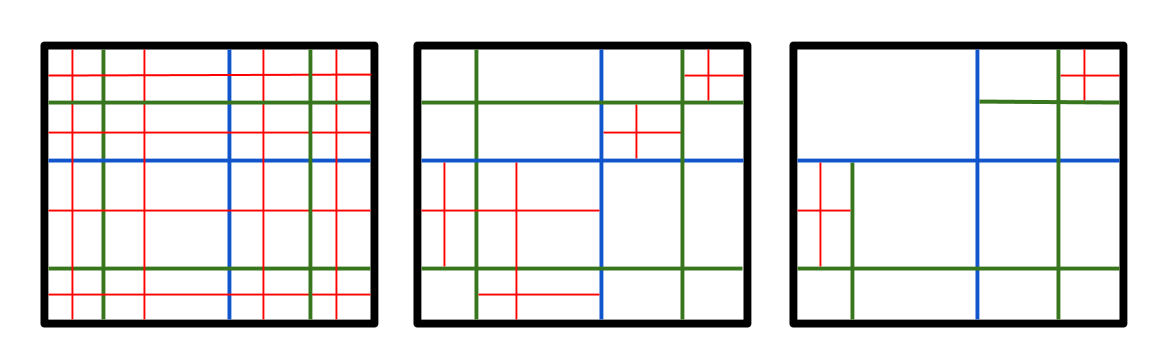
Figure 1: Example of two iterations of the merging algorithm on the partitions. The left sub-figure displays the hierarchical partitioning of $\mathbb{R}^{2}$ in the beginning. The level-$1$ rectangles are bordered by the blue lines, the level-$2$ by the green, and the level-$3$ by the red. In the first iteration, the candidates for merging are the groups of $4$ rectangles bordered by red. The center figure shows the results after the merging has been completed — the algorithm chooses to merge those that reduce the regularized error of (2). The right-most figure shows another iteration of the algorithm.

The regularized error measure is used as a proxy for the true error, which we cannot measure. We do not merge together rectangles that give the largest regularized error measure, since this is an indication that these samples might not fit well in a piece. By not merging $2k^{\prime}$ of the largest errors in each iteration, we have a guarantee that $k^{\prime}$ of these were actually rectangles on which $f$ was flat (contained in a true piece of $f$), which will allow us to bound the error on the rectangles we merge.

MultidimGreedyMerging$(\mathbf{X},\mathbf{y})$

Let $\mathcal{G}$ be a grid over the first $d^{\prime}$ coordinates of the samples in $\mathbf{X}$

Let $\mathcal{T}$ be a subtree of the hierarchical tree induced by $G$, initially containing all nodes which contain samples.

Let $\mathcal{S}$ be the collection of sets of sibling leaf nodes in $\mathcal{T}$.

Let $k^{\prime}=k\log^{d^{\prime}}n$

while $|\mathcal{S}|\geq 2k^{\prime}$ do

       for each set of sibling leaves $R\in\mathcal{S}$ do

             Let $\hat{f}_{R}$ = LeastSquares($\kappa({\mathbf{X}_{R}}),\mathbf{y}_{R}$)

             Let $\widetilde{\mathrm{err}}(R,\hat{f}_{R})=\|y_{R}-\hat{f}_{R}\|_{2}^{2}-\sigma^{2}|R|$

       end for

      Let $\mathcal{J}$ be the set of $2k^{\prime}$ sibling sets $R\in\mathcal{T}$ with largest $\widetilde{\mathrm{err}}(R,\hat{f}_{R})$

       for each $R\notin\mathcal{J}$ do

             Merge the sibling leaf nodes together in $\mathcal{T}$, so their parent becomes a leaf node

       end for

      

end while

return The function which is the least squares fit for every leaf of $\mathcal{T}$

Algorithm 1 Piecewise linear regression by greedy merging

3.1 Analysis of Algorithm 1

In our algorithm, we use the blackbox subroutine $\textsc{LeastSquares}(\mathbf{X},\mathbf{y})$, where $\mathbf{X}$ is the $n\times d$ data matrix and $\mathbf{y}$ is the vector of labels. The classical algorithms for least squares that are commonly used in practice have time complexity $O(nd^{2})$. We will assume this running time for this subroutine. So, when computing the least squares fit on some subrectangle $R$, $\textsc{LeastSquares}(\mathbf{X}_{R},\mathbf{y}_{R})$ runs in time $O(|R|\cdot d^{2})$. With this, it is not hard to show the following runtime bound.

Lemma 3.1.

Algorithm 1 runs in time $O(nd^{2}\log n)$.

Proof.

We go through a maximum of $\log n$ iterations. For each iteration, we need to call LeastSquares for each of the groups of sibling leaves in $\mathcal{T}$. For each group of leaves $S$, the runtime is $O(|S|\cdot d^{2})$, and since the leaves are disjoint, the total runtime over all the groups is $O(nd^{2})$. Thus, we get a runtime of $O(nd^{2}\log n)$ over all iterations. ∎

It is easily verified that by plugging in other solvers instead, we can also match their runtime, up to poly-logarithmic factors.

The following simple lemma bounds from above the number of pieces that the algorithm produces.

Lemma 3.2.

Algorithm 1 outputs a function that is piecewise linear on $O(k^{\prime\prime})$ pieces, where $k^{\prime\prime}=k\log^{d^{\prime}+1}n$.

Proof.

We stop merging if there are ever less than $2k^{\prime}$ sibling leaf groups under consideration to be merged. Each of these groups is responsible for preventing at most $2^{d^{\prime}}-1$ leaf nodes from being merged in each level on the path from them to the root node (since not all of the siblings of these leaves are also leaves). So, each group might block $2^{d^{\prime}}\log n$ leaf nodes from merging. Therefore, a total of $(2^{d^{\prime}}\log n)k^{\prime}=2^{d^{\prime}}k^{\prime\prime}$ leaf nodes are blocked, where $k^{\prime\prime}=k\log^{d^{\prime}+1}n$. If we add $2^{d^{\prime}+1}k^{\prime}$nodes that were up for consideration but not merged, we then have $O(k^{\prime\prime})$ total leaf nodes at the end. ∎

We are now ready to prove our main theorem.

Theorem 3.3.

Let $\delta>0$ and let $\hat{f}$ be the estimator returned by MultidimGreedyMerging. Let $k^{\prime}=O(k\log^{d^{\prime}}n)$. Let $k^{\prime\prime}=O(k\log^{d^{\prime}+1}n)$ be the number of pieces in $\hat{f}$. Let $r=\mathrm{rank}(\kappa(\mathbf{X}))$. Then, with probability $1-\delta$, we have

$$\mathrm{MSE}(\hat{f})=O\bigg{(}\frac{\sigma^{2}k^{\prime\prime}(r+\log(n/\delta))}{n}+\frac{\sigma\sqrt{k^{\prime}}\log(n/\delta)}{\sqrt{n}}\bigg{)}\;.$$

Proof.

Let $\mathcal{R}=\{R_{1},\ldots,R_{k^{\prime\prime}}\}$ be the leaves output by the algorithm. We partition $\mathcal{R}$ into two sets, and bound the error on the sets separately. We say $f$ is flat on a rectangle $R$ if $f$ over $R$ is defined by one linear function. We say that $f$ has a jump on $R$ if it is defined by more than one linear function over $R$. Let $\mathcal{F}=\{R\in\mathcal{R}:\text{f is flat on R}\}$ and $\mathcal{J}=\{R\in\mathcal{R}:\text{f has a jump on R}\}$.

We can bound the error over the rectangles in $\mathcal{F}$ by directly applying Lemma 2.6 to get $\sum_{R\in\mathcal{F}}\mathrm{err}(R)\leq O(\sigma^{2}k^{\prime\prime}(r+\log(n/\delta)))$. Next we bound the error of the rectangles in $\mathcal{J}$. Consider some $R\in\mathcal{J}$. If $|R|=1$, call this set $\mathcal{J}_{1}$. Then we know that $\hat{f}(x_{i})=y_{i}$ for the $i\in R$. We get the following bound from Lemma 2.4.

$$\sum_{R\in\mathcal{J}_{1}}\|\mathbf{f}_{R}-\hat{\mathbf{f}}_{R}\|^{2}_{2} \leq\sum_{R\in\mathcal{J}_{1}}\|\boldsymbol{\epsilon}_{R}\|^{2}_{2}$$

$$\leq O\left(\sum_{R\in\mathcal{J}_{1}}|R|+\log(n/\delta)\sqrt{|R|}\right)$$

$$\leq O\left(\sigma^{2}\left(k^{\prime\prime}+\log(n/\delta)\sqrt{k^{\prime\prime}}\right)\right)\;.$$

Otherwise, $R\in\mathcal{J}$ but $|R|>1$. Call this set $\mathcal{J}_{2}$. So, for each $R\in\mathcal{J}_{2}$, there was some iteration where there was a rectangle $R^{\prime}$ such that $R^{\prime}\subseteq R$, and $R^{\prime}$ was merged in that iteration. Let the set of rectangles that were sub-rectangles of rectangles in $\mathcal{J}_{2}$ and were merged at some iteration be $\mathcal{R}^{\prime}$.

In an iteration where $R^{\prime}$ was merged, there were $2k^{\prime}$ rectangles, $R_{1},\dots,R_{2k^{\prime}}$ such that $\widetilde{\mathrm{err}}(R^{\prime})\leq\widetilde{\mathrm{err}}(R_{j})$ for $j=1,\ldots,2k^{\prime}$. Out of these, we know that on at least $k^{\prime}$ of them, $f$ must be flat. Let this set be $\mathcal{R}^{*}$. We know that the error of each $R\in\mathcal{R}^{*}$ can be bounded above by the average error of all $R\in\mathcal{R}^{*}$. So, we have that $\widetilde{\mathrm{err}}(R^{\prime})\leq\widetilde{\mathrm{err}}(R_{j})\leq\tfrac{1}{k^{\prime}}\sum_{R\in\mathcal{R}^{*}}\widetilde{\mathrm{err}}(R)$.

We can bound $\sum_{R\in\mathcal{R}^{*}}\widetilde{\mathrm{err}}(R)$ as follows

$$\sum_{R\in\mathcal{R}^{*}}\widetilde{\mathrm{err}}(R) =\sum_{R\in\mathcal{R}^{*}}\|\mathbf{y}_{R}-\hat{\mathbf{f}}_{R}\|_{2}^{2}-\sigma^{2}|R|$$ (3)

$$=\sum_{R\in\mathcal{R}^{*}}\|\mathbf{f}_{R}-\hat{\mathbf{f}}_{R}\|^{2}_{2}$$

$$~{}~{}~{}~{}+2\sum_{R\in\mathcal{R}^{*}}\langle\boldsymbol{\epsilon}_{R},\mathbf{f}_{R}-\hat{\mathbf{f}}_{R}\rangle$$

$$~{}~{}~{}~{}+\sum_{R\in\mathcal{R}^{*}}\sum_{i\in R}(\varepsilon_{i}^{2}-\sigma^{2})$$ (4)

$$\leq O(\sigma^{2}k^{\prime}(r+\log(n/\delta)))$$

$$~{}~{}~{}~{}+O(\sigma\log(n/\delta)\sqrt{n})\;.$$ (5)

The first term in (5) follows from bounding the first term of (4) with Lemma 2.6, and the second term of (4) with Lemma 2.5. The second term of (5) follows from Lemma 2.4.

Thus, we divide by $k^{\prime}$ to get that $\widetilde{\mathrm{err}}(R^{\prime})\leq O(\sigma^{2}(r+\log(n/\delta)))+O(\frac{1}{k^{\prime}}\sigma\log(n/\delta)\sqrt{n})$. Since we actually want to bound $\mathrm{err}(R^{\prime})$, we bound from below $\widetilde{\mathrm{err}}(R^{\prime})$:

$$\widetilde{\mathrm{err}}(R^{\prime}) =\|\mathbf{y}_{R^{\prime}}-\hat{\mathbf{f}}_{R^{\prime}}\|^{2}_{2}-\sigma^{2}|R^{\prime}|$$

$$=\|\mathbf{f}_{R^{\prime}}-\hat{\mathbf{f}}_{R^{\prime}}\|^{2}_{2}$$

$$~{}~{}~{}~{}+2\langle\varepsilon_{R^{\prime}},\mathbf{f}_{R}-\hat{\mathbf{f}}_{R}^{\prime}\rangle+(\|\varepsilon_{i}\|^{2}_{2}-\sigma^{2}|R^{\prime}|)$$

$$\geq\mathrm{err}(R^{\prime})-O(\sigma\sqrt{r+\log(n/\delta)})\|\mathbf{f}_{R^{\prime}}-\hat{\mathbf{f}}_{R^{\prime}}\|_{2}$$

$$~{}~{}~{}~{}-O(\sigma\log(n/\delta))\sqrt{|R^{\prime}|}\;,$$

where the second term is bounded by Lemma 2.5 and the last term is bounded by Lemma 2.4.

We combine this bound with (4) and rearrange to get

$$\mathrm{err}(R^{\prime}) \leq O(\sigma^{2}(r+\log(n/\delta)))$$

$$~{}~{}~{}~{}+O(\sigma\sqrt{r+\log(n/\delta)})\|\mathbf{f}_{R^{\prime}}-\hat{\mathbf{f}}_{R^{\prime}}\|_{2}$$

$$~{}~{}~{}~{}+O\left(\sigma\log(n/\delta)(\sqrt{|R^{\prime}|}-\frac{\sqrt{n}}{k^{\prime}})\right)\;.$$

This inequality is of the form $z^{2}\leq bz+c$, where $b,c>0$, so then $z^{2}\leq O(b^{2}+c)$. Thus, we have

$$\mathrm{err}(R^{\prime})\leq O(\sigma^{2}(r+\log(n/\delta)))+$$

$$O\left(\sigma\log(n/\delta)(\sqrt{|R^{\prime}|}+\frac{\sqrt{n}}{k^{\prime}})\right)\;.$$

Therefore, the total error for rectangles in $\mathcal{J}_{2}$ is

$$\sum_{R\in\mathcal{J}_{2}}\mathrm{err}(R)\leq\sum_{R^{\prime}\in\mathcal{R}^{\prime}}\mathrm{err}(R^{\prime})$$

$$\leq O(\sigma^{2}k^{\prime}(r+\log(n/\delta)))+O(\sigma\log(n/\delta))(\sqrt{k^{\prime}n}),$$

where the second term follows from the fact that the rectangles in $\mathcal{R}^{\prime}$ are disjoint. Summing up the bounds we get for $\mathcal{F},\mathcal{J}_{1},$ and $\mathcal{J}_{2}$ completes the proof. ∎

4 Experiments

We study the performance of our new estimator for segmented regression on both synthetic and real data. All experiments were done on a laptop computer with a 2.5 GHz Intel Core i5 CPU and 8 GB of RAM. The focus of these evaluations was on statistical accuracy, not time efficiency. However, we note that the runtime of our algorithm was similar to that of CART. All algorithms took at most 18 seconds to run on the above computer architecture. For our synthetic data evaluations with piecewise constant true functions, our algorithm performs better in this measure. On real datasets, while our piecewise constant fits are worse than CART, we can perform better than CART if we use the full power of our estimator and output a piecewise linear predictor. Code of our implementation and experiments is available at https://github.com/avoloshinov/multidimensional-segmented-regression.

Synthetic data

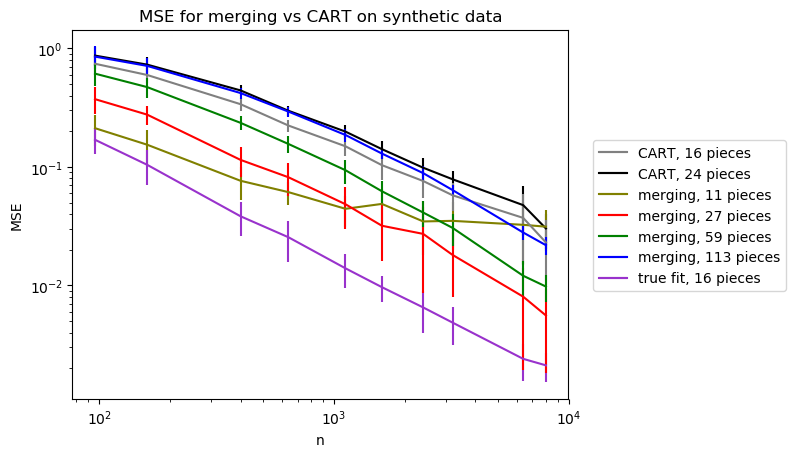
Figure 2: MSE of the merging algorithm and CART on synthetic data. There are four versions of our algorithm “merging” shown, with the average number of pieces that the algorithm produced over all of the trials over all of the values of $n$. There are two versions of CART shown — one that was limited to producing $16$ pieces, and one that was limited to producing $24$ pieces. The “true fit” shows what the piecewise constant fit is on the true partition with $16$ pieces.

We first compare the statistical performance of our algorithm to CART on synthetic data. We used the ScikitLearn Julia library to import the DecisionTreeRegressor model from the Python skikit-learn library. This model implements CART (https://scikit-learn.org/stable/modules/tree.html#tree).

Since we are comparing to CART, which produces piecewise constant predictors, we consider the special case of our algorithm using constant predictors, to give the fairest comparison. Observe that this corresponds to the special case of the constant kernel $\kappa(\textbf{x})=1$. We generate a function $f$ that is piecewise constant in $d^{\prime}=2$ dimensions with a total of $d=10$ features. To generate the data, we draw $n$ (ranging from $n=96$ to $n=8000$) samples, where each coordinate is a normally-distributed random number with mean $0$ and standard deviation $1$. We then generate a piecewise constant function with $k=16$ pieces in $d^{\prime}=2$ dimensions, by uniformly partitioning the data in the first two coordinates, such that each piece contains $n/k$ samples. Then, we pick a constant function for each piece, independently and uniformly at random from the interval $[0,1]$. We add i.i.d Gaussian noise with variance $1$ to each sample.

Figure 2 shows the average MSE over $20$ trials. The “true fit” shows the error of fitting a constant function on each of the true pieces. We ran CART with $16$ as the maximum number of leaves, as well as $24$ as the maximum number of leaves. We ran our algorithm “merging” with four different parameter settings, which resulted in an average of $11$, $27$, $59$, and $113$ pieces, for parameter settings respectively of $k,k/2,k/4,$ and $k/8$ for the number of candidate sets left when we stop merging. In theory, this parameter should be $2k^{\prime}$, where $k^{\prime}=k\log^{2}n$, but in practice, setting this parameter to smaller values and allowing our tree to keep merging works better, to a certain point. Most of our parameter settings achieved lower error than both of the CART algorithms for all values of $n$.

Real data

We investigate how our algorithm performs on real data through the Boston dataset (https://www.cs.toronto.edu/~delve/data/boston/bostonDetail.html). This dataset consists of $506$ samples, where each sample has $14$ attributes — we use the first $13$ as features and the last as the label. The goal is to model the median value of owner-occupied homes in $1000$s of dollars. We chose this dataset because it is presented as the main example in the documentation for CART in scikit-learn (https://scikit-learn.org/stable/modules/generated/sklearn.tree.DecisionTreeRegressor.html), as well as in many other examples of CART.

First, we compare the performance of CART on this dataset with a piecewise constant version of our algorithm (i.e., using the constant kernel). We run our algorithm and use the output of the number of pieces (25) as the input for how many pieces we want CART to output. For the merging algorithm, we use $4$ as the stopping parameter for merging, and $4$ as the value for sigma. We compute the model based on all of the samples, and then look at the MSE of the model on all of the samples.

For the stopping parameter, we tried values of $1,2,3,4,5,6$, which resulted in piecewise fits ranging from $7$ pieces to $54$ pieces. The choice for this parameter depends on the desired succinctness of the model. Since the comparisons to CART are similar for different value of this parameter, we just show the results for a single parameter. With a fixed stopping parameter (4), we tried $1,2,3,4,5,10$ as values for sigma, representing the variance of the noise of the data. We used these parameters and ran our algorithm on the data, then used the value that gave the best MSE on the data. We note that as a result of our choice of $\sigma$, the MSE only differed by a maximum of $7$, and usually by only $1$-$2$.

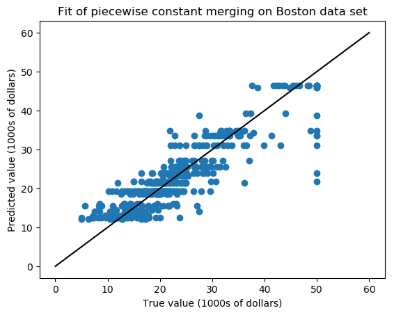
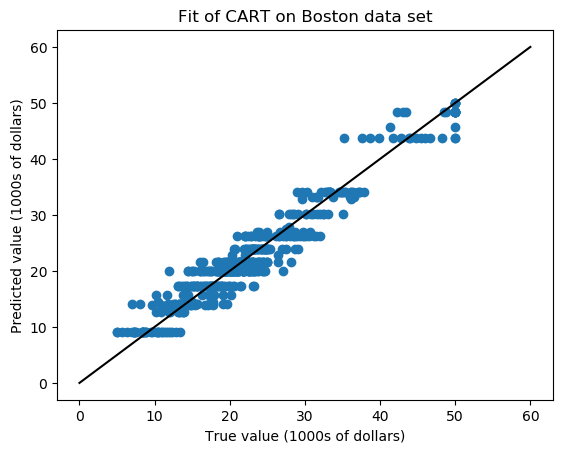
Figure 3: The piecewise constant fit with $25$ pieces with the merging algorithm and CART. The merging algorithm split on $2$ features: lstat (percent lower status of the population) and rm (average number of rooms per dwelling). The MSE of the merging algorithm was $19.242$ and the MSE of CART was $6.155$.

Now, we look at the performance of CART on this dataset with the piecewise linear version of our algorithm (i.e., the identity kernel function $\kappa(\textbf{x})=\textbf{x}$). Similarly to the constant experiment, we first run our algorithm, and use the output of the number of pieces as the input for how many pieces we want CART to output. For the merging algorithm, we use $3$ as the stopping parameter for merging, and $2$ as the value for sigma, which were chosen in the same manner as before. We compute the model based on all of the samples, and then look at the MSE of the model on all of the samples.

While our piecewise constant algorithm produced a result with worse MSE than CART, we can see that using our linear predictor can produce results with better MSE than CART in multiple regimes. We also note that our linear predictor, with sigma set between $1$ and $3$, outperforms CART for all stopping parameters that we chose, resulting in piecewise outputs on $7$ to $54$ pieces.

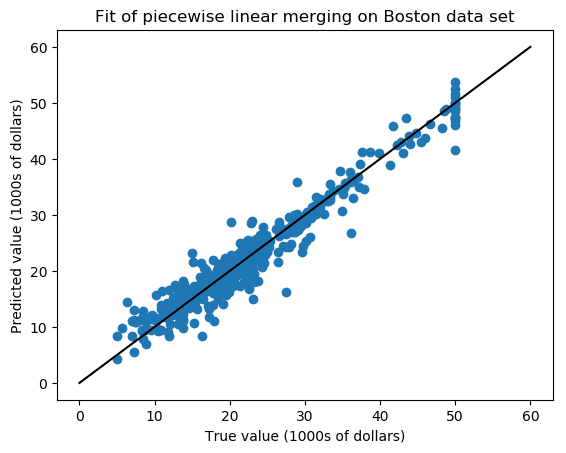
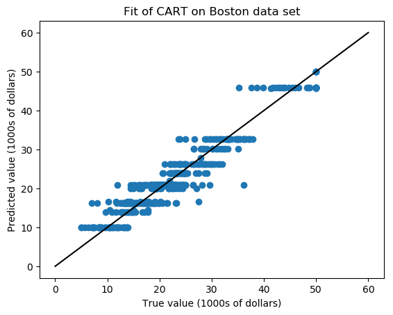
Figure 4: The linear constant fit with $16$ pieces with the merging algorithm, and a $16$ piece constant fit with CART. The merging algorithm split on $2$ features: lstat (percent lower status of the population) and rm (average number of rooms per dwelling). The MSE of the merging algorithm was $5.464$ and the MSE of CART was $8.615$.

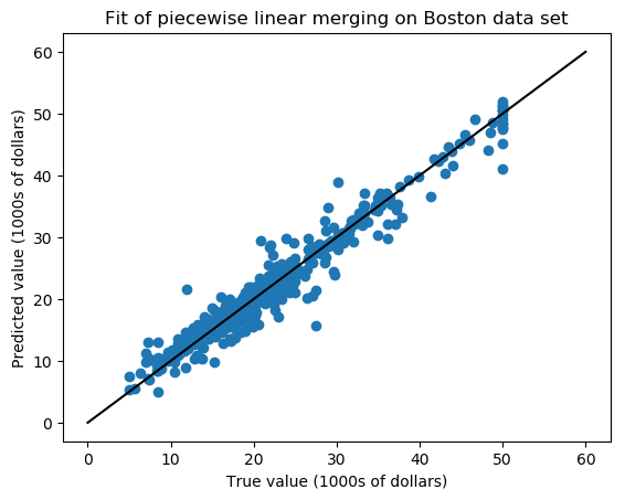
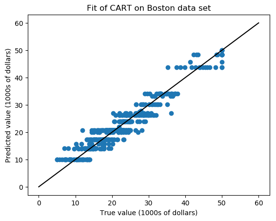
Figure 5: The linear constant fit with $22$ pieces with the merging algorithm, and a $22$ piece constant fit with CART. The merging algorithm split on $3$ features: lstat (percent lower status of the population), rm (average number of rooms per dwelling), and dis (weighted distances to five Boston employment centers). The MSE of the merging algorithm was $4.303$ and the MSE of CART was $6.779$.

Appendix A Omitted Details from Section 2

A.1 Proof of Lemma 2.5

Before we prove the lemma, we need the following maximal inequality, which bounds the correlation of a random vector with any fixed $d$-dimensional subspace, and the corollary bounds the correlation between sub-Gaussian random noise and any linear function on any rectangle.

Lemma A.1 (see e.g., proof of Theorem 2.2 in [Rig15]).

Fix $\delta>0$ and $\mathbf{v}\in\mathbb{R}^{n}$. Let $\varepsilon_{1},\ldots,\varepsilon_{n}$ be as defined in (1). Let $\boldsymbol{\epsilon}=(\varepsilon_{1},\ldots,\varepsilon_{n})$, and let $S$ be a fixed, $r$-dimensional affine subspace of $\mathbb{R}^{n}$. Then, with probability $1-\delta$, we have

$$\sup_{v\in S\setminus\{0\}}\frac{|\langle\boldsymbol{\epsilon},\mathbf{v}\rangle|}{\|\mathbf{v}\|_{2}}\leq O(\sigma\sqrt{r+\log(1/\delta)})\;.$$

With this lemma in hand we can now prove Lemma 2.5,

Proof of Lemma 2.5.

Fix a partition of $[0,1]^{2}$ into $k^{\prime}$ rectangles $\mathcal{R}$, where each $R\in\mathcal{R}$ is such that $R\in\mathcal{T}$. Let $S_{\mathcal{R}}$ be the set of $k^{\prime}$-piecewise linear functions, which are linear fits on each $R\in\mathcal{R}$. Then, $S_{\mathcal{R}}$ is a $k^{\prime}\cdot\mathrm{rank}(\kappa(\mathbf{X}))$-dimensional affine subspace. By Lemma A.1,

$$\sup_{f\in S_{\mathcal{R}}}\frac{|\langle\boldsymbol{\epsilon}_{R},\mathbf{f}_{R}\rangle|}{\|\mathbf{f}_{R}\|_{2}}\leq O(\sigma\sqrt{k^{\prime}\mathrm{rank}(\kappa(\mathbf{X}))+\log(1/\delta^{\prime})})\;,$$

with probability $1-\delta^{\prime}$. The number of possible partitions $\mathcal{R}$ is bounded above by ${n^{2}\choose{k^{\prime}}}=O(n^{2k^{\prime}})$. Let $\delta^{\prime}=\delta/n^{2k^{\prime}}$, then the result follows from a union bound over all possible partitions. ∎

A.2 Proof of Lemma 2.6

By the definition of the least squares fit, we have that $\left\|\mathbf{y}_{\mathcal{R}}-\hat{\mathbf{f}}_{\mathcal{R}}\right\|^{2}_{2}\leq\left\|\mathbf{y}_{\mathcal{R}}-\mathbf{f}_{\mathcal{R}}\right\|^{2}_{2}=\left\|\boldsymbol{\epsilon}_{\mathcal{R}}\right\|^{2}_{2}.$ If we expand the left hand side we get

$$\left\|\mathbf{y}_{\mathcal{R}}-\hat{\mathbf{f}}_{\mathcal{R}}\right\|^{2}_{2}=\left\|\mathbf{f}_{\mathcal{R}}+\boldsymbol{\epsilon}_{\mathcal{R}}-\hat{\mathbf{f}}_{\mathcal{R}}\right\|^{2}_{2}=\left\|\hat{\mathbf{f}}_{\mathcal{R}}-\mathbf{f}_{\mathcal{R}}\right\|^{2}_{2}+2\langle\boldsymbol{\epsilon}_{\mathcal{R}},\mathbf{f}_{\mathcal{R}}-\hat{\mathbf{f}}_{\mathcal{R}}\rangle+\left\|\boldsymbol{\epsilon}_{\mathcal{R}}\right\|^{2}_{2}\;.$$ (6)

Applying Lemma 2.5 gives us that with probability $1-\delta$,

$$\left\|\hat{\mathbf{f}}_{\mathcal{R}}-\mathbf{f}_{\mathcal{R}}\right\|^{2}_{2} \leq 2\langle\boldsymbol{\epsilon}_{\mathcal{R}},\hat{\mathbf{f}}_{\mathcal{R}}-\mathbf{f}_{\mathcal{R}}\rangle$$

$$\leq O(\sigma\sqrt{k^{\prime}\cdot\mathrm{rank}(\kappa(\mathbf{X}))+k^{\prime}\log(n/\delta)})\left\|\hat{\mathbf{f}}_{\mathcal{R}}-\mathbf{f}_{\mathcal{R}}\right\|_{2}\;.$$

Rearranging this, we get that $\left\|\hat{\mathbf{f}}_{\mathcal{R}}-\mathbf{f}_{\mathcal{R}}\right\|^{2}_{2}\leq O(\sigma^{2}k^{\prime}\mathrm{rank}(\kappa(\mathbf{X})+k^{\prime}\log(n/\delta))$, which is what we wanted to show.

References

- [ADH+15] J. Acharya, I. Diakonikolas, C. Hegde, J. Z. Li, and L. Schmidt. Fast and near-optimal algorithms for approximating distributions by histograms. In PODS, pages 249–263, 2015.
- [ADLS16] J. Acharya, I. Diakonikolas, J. Li, and L. Schmidt. Fast algorithms for segmented regression. In Proceedings of the 33nd International Conference on Machine Learning, ICML 2016, pages 2878–2886, 2016.
- [ADLS17] J. Acharya, I. Diakonikolas, J. Li, and L. Schmidt. Sample-optimal density estimation in nearly-linear time. In Proceedings of the Twenty-Eighth Annual ACM-SIAM Symposium on Discrete Algorithms, SODA 2017, pages 1278–1289, 2017. Available at https://arxiv.org/abs/1506.00671.
- [ASW13] H. Avron, V. Sindhwani, and D. Woodruff. Sketching structured matrices for faster nonlinear regression. In NIPS, pages 2994–3002. 2013.
- [BFOS84] L. Breiman, J.H. Friedman, R.A. Olshen, and C.J. Stone. Classification and regression trees. wadsworth & brooks. Cole Statistics/Probability Series, 1984.
- [BP98] J. Bai and P. Perron. Estimating and testing linear models with multiple structural changes. Econometrica, 66(1):47–78, 1998.
- [BSRM07] G. Blanchard, C. Schäfer, Y. Rozenholc, and K. R. Müller. Optimal dyadic decision trees. Machine Learning, 66(2-3):209–241, 2007.
- [CGS15] S. Chatterjee, A. Guntuboyina, and B. Sen. On risk bounds in isotonic and other shape restricted regression problems. Annals of Statistics, 43(4):1774–1800, 08 2015.
- [DLS18] I. Diakonikolas, J. Li, and L. Schmidt. Fast and sample near-optimal algorithms for learning multidimensional histograms. In Conference On Learning Theory, COLT 2018, pages 819–842, 2018.
- [EH89] A. Ehrenfeucht and D. Haussler. Learning decision trees from random examples. Information and Computation, 82(3):231–246, 1989.
- [Fed75] P. I. Feder. On asymptotic distribution theory in segmented regression problems– identified case. Annals of Statistics, 3(1):49–83, 01 1975.
- [Fri91] J. H. Friedman. Multivariate adaptive regression splines. Annals of Statistics, 19(1):1–67, 03 1991.
- [GA73] A. R. Gallant and Fuller W. A. Fitting segmented polynomial regression models whose join points have to be estimated. Journal of the American Statistical Association, 68(341):144–147, 1973.
- [HHZ06] T. Hothorn, K. Hornik, and A. Zeileis. Unbiased recursive partitioning: A conditional inference framework. Journal of Computational and Graphical statistics, 15(3):651–674, 2006.
- [KRS15] R. Kyng, A. Rao, and S. Sachdeva. Fast, provable algorithms for isotonic regression in all -norms. In NIPS, pages 2701–2709, 2015.
- [Loh02] W. Y. Loh. Regression tress with unbiased variable selection and interaction detection. Statistica Sinica, pages 361–386, 2002.
- [Loh11] W. Y. Loh. Classification and regression trees. Wiley Interdisciplinary Reviews: Data Mining and Knowledge Discovery, 1(1):14–23, 2011.
- [Mey08] M. C. Meyer. Inference using shape-restricted regression splines. Annals of Applied Statistics, 2(3):1013–1033, 09 2008.
- [MT77] F. Mosteller and J. W. Tukey. Data analysis and regression: a second course in statistics. Addison-Wesley, Reading (Mass.), Menlo Park (Calif.), London, 1977.
- [Q+] J. R. Quinlan et al. Learning with continuous classes. World Scientific.
- [Rig15] P. Rigollet. High dimensional statistics. 2015.
- [YP13] Y. Yamamoto and P. Perron. Estimating and testing multiple structural changes in linear models using band spectral regressions. Econometrics Journal, 16(3):400–429, 2013.