Analysis and Control of Power-Temperature Dynamics in Heterogeneous Multiprocessors

Abstract

Virtually all electronic systems try to optimize a fundamental trade-off between higher performance and lower power consumption. The latter becomes critical in mobile computing systems, such as smartphones, which rely on passive cooling. Otherwise, the heat concentrated in a small area drives both the junction and skin temperatures up. High junction temperatures degrade the reliability, while skin temperature deteriorates the user experience. Therefore, there is a strong need for a formal analysis of power consumption-temperature dynamics and predictive thermal management algorithms. This paper presents a theoretical power-temperature analysis of multiprocessor systems, which are modeled as multi-input multi-output dynamic systems. We analyze the conditions under which the system converges to a stable steady-state temperature. Then, we use these models to design a control algorithm that manages the temperature of the system without affecting the performance of the application. Experiments on the Odroid-XU3 board show that the control algorithm is able to regulate the temperature with a minimal loss in performance when compared to the default thermal governors.

I Introduction

The performance and capabilities of state-of-the-art mobile processors are severely limited by heat dissipation and resulting chip temperature [1, 2]. Competitive performance and functionality are enabled by increasing the operating frequency and the number of processing cores [3]. These choices lead to higher device temperature, thus affecting both user experience and reliability [1, 2, 4]. Therefore, maximum temperature constrains the power consumption, which limits the maximum operating frequency and number of active cores [5]. Commercial mobile platforms typically have hard-coded maximum safe temperature limits [6, 7]. If the temperature exceeds this limit at runtime, the system throttles the operating frequencies or reduces the number of active cores to decrease the temperature. In extreme cases, the system performs an emergency shutdown, which further cripples the performance and user experience [4].

Power consumption and temperature form a well-known positive feedback system [8, 9]. An increase in power consumption leads to an increase in temperature due to thermal resistance and capacitance networks [10]. As a result of the increase in temperature, there is an exponential rise in the leakage power [11]. If the system dynamics is stable, there exists a fixed-point temperature to which all the temperature trajectories converge within the region of convergence. That is, the temperature and power consumption rise until they eventually reach a fixed-point temperature. In contrast, an unstable system leads to a thermal runaway [9, 8, 12].

The stability of the system and existence of a fixed point do not necessarily ensure a thermally safe operation [12, 9]. The stable fixed point may lie beyond the temperature at which the system starts to throttle the frequencies or it may be greater than the operating limit of the device. Moreover, in a multiprocessor system, each core can converge to a different fixed-point temperature due to interactions between the core and workload running on each core [13]. For instance, if the graphics processing unit (GPU) is not heavily utilized, it converges to a lower temperature than heavily utilized cores. Therefore, the stable fixed point for each temperature hotspot has to be evaluated at runtime as the workload changes, so that necessary actions can be taken when violations are detected.

This paper presents a theoretical analysis of power-temperature dynamics in mobile multiprocessor systems. We start with an overview of power and thermal models used in the analysis. Then, we present an efficient method to evaluate the stability of the system and compute its fixed points. This is followed by a detailed analysis of the region of convergence of the thermal dynamics in a mobile multiprocessor system. Finally, we present a control algorithm to illustrate how we can avoid thermal violations. The control algorithm uses the fixed-point predictions to determine if the power-temperature dynamics is within a safe region of operation. If any violations are detected, it reduces the frequency for the application that is causing thermal violation. The selective control ensures that other applications in the system are not penalized. We evaluate the control algorithm on the Odroid-XU3 [14] platform. The platform includes the Exynos-5422 big.Little System-on-a-Chip (SoC). We use this platform for our experimental evaluations since it is used on smartphones like Samsung Galaxy S5 and is representative of the processors used in mobile systems. Our experiments on the Odroid-XU3 platform show that the proposed algorithm is able to isolate the power-hungry application, while maintaining the performance requirements of active applications. In summary, the major contributions of this paper are:

• An efficient solution to find the region of convergence of the power-temperature dynamics in a multiprocessor system,

• An optimization technique that speeds up the computation of the fixed point by up to 1.8$\times$ when compared to a baseline approach used in [12],

• A low-overhead control algorithm that uses fixed-point analysis to prevent thermal violations and lower the power consumption. Implementation on a commercial device shows that the algorithm is effective in preventing thermal violations while also lowering the power consumption of the device.

Application domains of proposed analysis: The primary application area of the proposed analysis is low-power handheld and wearable devices where the skin temperature of the device is critical for user comfort. This is especially important in wearable devices where the device is in constant contact with the user’s body. We can use the proposed analysis to predict the steady-state temperature of the device when a user is running an application over long periods of time (such as playing a game). Then, we can use the predictions and the time to reach the steady state to determine if the current trajectory leads to high skin-temperature and user discomfort. We also note that the proposed analysis and the control algorithm are not directly applicable to high-performance server units where the power consumption may change in the order of milliseconds.

The rest of the paper is organized as follows. We review the related work in Section II. Section III presents an overview of the temperature and power models used in the fixed-point analysis. Section IV first presents an overview of the fixed-point prediction for a single-input-single-output (SISO) model. This is followed by our analysis of the general multiple-input-multiple-output (MIMO) model. The lightweight control algorithm using fixed-point predictions is presented in Section V. Finally, we present the experimental evaluations in Section VI and the conclusions in Section VII.

II Related Work

Higher power densities in modern multiprocessors has led to increasing thermal stress on these devices. Higher temperature has an adverse impact on reliability [8, 15]. Therefore, a significant amount of research has focused on accurate, yet complex, offline models and lightweight runtime models. Design-time studies focus on analyzing the full-chip thermal behavior under different application workloads such that thermal policies for the chip can be determined [1, 16]. Since they simulate traces from common workloads to model the static and transient thermal behavior, they are not amenable to runtime analysis. In contrast, runtime approaches develop computationally efficient thermal and power models, which can be used for runtime analysis of the system [17, 12]. For instance, a grey-box system identification is used in [17] to develop the thermal model of a multicore system. A recent approach proposed in [12] performs an analysis of the stability of power-temperature dynamics in multiprocessor systems. However, it uses a simplified SISO model for evaluating the region of convergence of the power-temperature dynamics. In contrast, this paper presents an efficient solution to find the region of convergence of the power-temperature dynamics using a MIMO model.

MIMO system identification techniques have also been used in dynamic power management of multiprocessor systems [18, 19]. For instance, the work in [18] uses a MIMO formulation to model the queue utilizations in a multiprocessor system with multiple voltage-frequency islands. Then, it uses a feedback control algorithm to determine the operating frequency and voltage of each island while maintaining a reference utilization for each queue. Similarly, the approach in [19] first models the workload characteristics in a multiprocessor system using a multi-fractal master equation. Then, it uses the equation in a model predictive control algorithm to perform dynamic voltage and frequency scaling. Complementary to these approaches, the MIMO system identification used in this paper models the temperature of the device as a function of the power consumption of the different components in the system while not considering the specific workload characteristics. Therefore, we can potentially combine our models with the MIMO approaches of prior work [18, 19] to enable workload-aware thermal and power management.

Commercial products come with a mechanism to control the temperature of the system. It is achieved either by throttling the performance or shutting down the system. Reactive approaches continuously monitor the temperature and respond to avoid thermal violations, resulting in a larger penalty on performance [13, 20]. To mitigate the performance penalty, recent research has focused on developing predictive approaches for dynamic thermal and power management (DTPM). Predictive approaches develop computationally efficient thermal and power models [17, 21]. These models are used at runtime to estimate the short-term behavior of the power-temperature dynamics and take actions if violations are predicted [22, 23, 21]. These approaches are effective in predicting the short-term behavior of the power-temperature dynamics; however, the prediction error increases when long-term predictions are made [23]. A number of studies have also used control-theoretic approaches to regulate the temperature of the system [24, 25, 26, 27]. For instance, the work in [24] uses an integral controller to regulate the temperature of the system. The authors consider a nonlinear thermal model that captures the exponential dependence on leakage power. Similarly, the authors in [26] use an event-based proportional integral controller to maintain the temperature of the system below a desired set point. These approaches implement control algorithms around a desired set point. If the temperature reaches this set point, they throttle the whole system to decrease the power consumption and regulate the temperature. This, however, can cripple the whole system performance and penalize all active applications. In contrast, our stability analysis technique predicts the steady-state temperature before a thermal violation occurs. Hence, it can assist thermal management by predicting the steady-state temperature and enabling proactive decisions.

Positive feedback between the power consumption and temperature has been analyzed by a number of studies [9, 28, 12]. For instance, Liao et al. [9] show that a positive second-order derivative of the temperature leads to a thermal runaway. This criterion can be easily used for design-time analysis of the chip. However, it is not practical to use it at runtime, since the condition is true only after a thermal runaway has started. Temperature dependence of leakage current is used in [28] to increase the thermally sustainable power of the chip. The work in [12] proposes an approach to analyze the existence of fixed points by first reducing the system to a SISO model. However, none of these techniques can analyze the existence and stability of fixed points at runtime while considering the coupling between different cores. This paper presents a theoretical methodology to overcome this limitation and provides an efficient algorithm to calculate the fixed points and their stability. The fixed points are then used in a simple control algorithm that can avoid thermal violations without excessive performance penalties. The fixed-point analysis can also be used as an effective guard against power attacks, which cause damage by increasing the temperature of the device [29, 30, 31].

III Background and Overview

This section presents the power consumption and temperature models required for the proposed thermal fixed-point analysis. We provide an overview here for completeness, while additional details are presented in [21, 12].

III-A Power and Temperature Models

Let us assume that there are $M$ processors in the system, as summarized in Table I. The power consumption of processors in the target system is given by the $M\times 1$ vector $\mathbf{P}=[P_{1},P_{2},\ldots,P_{M}]^{\text{T}}$, where $P_{i}$ is given by:

$$P_{i}=C_{sw,i}V_{i}^{2}f_{i}+V_{i}I_{g,i}+V_{i}\kappa_{1,i}T_{i}^{2}e^{\frac{\kappa_{2,i}}{T_{i}}},~{}~{}1\leq i\leq M.$$ (1)

where $C_{sw,i}$ is the switching capacitance, $V_{i}$ is the supply voltage and $f_{i}$ is the operating frequency, $I_{g,i}$ is the gate leakage, $\kappa_{1,i}>0$ and $\kappa_{2,i}<0$ are technology-dependent parameters, and $T_{i}$ is the temperature. Since our focus is to analyze the dependence of power on the temperature, we can isolate the impact of the temperature as

$$P_{i}=P_{C,i}+V_{i}\kappa_{1,i}T_{i}^{2}e^{\frac{\kappa_{2,i}}{T_{i}}},~{}~{}1\leq i\leq M,$$ (2)

where $P_{C,i}=C_{sw,i}V_{i}^{2}f_{i}+V_{i}I_{g,i}$ represents the temperature-independent component.

Assume that are $N$ thermal hotspots in the system. The temperature of each thermal hotspot can be written as a function of the power consumption vector $\mathbf{P}$ and thermal capacitance and conductance matrices [1, 10]. Therefore, the temperature dynamics is defined by the state-space system

$$\mathbf{T[k+1]}=\mathbf{A}\mathbf{T[k]}+\mathbf{B}\mathbf{P[k]}$$ (3)

where $\mathbf{A}$ matrix is symmetric due to symmetricity of the heat transfer. A discrete-time system is used because temperature measurements and control decisions are sampled at equal discrete time intervals. Equation (3) expresses the temperature of each hotspot in the next time step as a function of the current temperature and the power consumption of $M$ sources. The $\mathbf{A}$ matrix describes the effect of temperature in time step $k$ on the temperature in the next time step. That is, it describes the coupling between the temperature hotspots. Similarly, the ${N\times M}$ matrix $\mathbf{B}$ describes the relation between the temperature in the next time step and each of the power sources. Substituting (1) in (3) leads to a system of nonlinear equations,

$$\mathbf{T[k+1]}=\mathbf{A}\mathbf{T[k]}+\mathbf{B}\big{[}P_{1}[k],P_{2}[k],\ldots,P_{M}[k]\big{]}^{\text{T}},~{}\mathrm{where}$$ (4)

$$\vspace{-2mm}P_{i}[k]=C_{sw,i}V_{i}^{2}f_{i}+I_{g,i}V_{i}+V_{i}\kappa_{1,i}T_{i}[k]^{2}e^{\frac{\kappa_{2,i}}{T_{i}[k]}},~{}1\leq i\leq M.$$

TABLE I: Summary of major parameters

Symbol	Description
$N,M$	The number of thermal hotspots and processing elements (resources) in the SoC, respectively.
$\mathbf{T[k]}$	$N\times 1$ vector where $T_{i}[k],~{}1\leq j\leq N$ denotes the temperature of the $i^{th}$ hotspot at time instant k.
$T$	The maximum (scalar) steady-state temperature over all thermal hotspots.
$\mathbf{P[k]}$	$M\times 1$ vector where $P_{i}[k],~{}1\leq i\leq M$ denotes the power consumption of the $i^{th}$ resource at time instant k.
$\kappa_{1,i},\kappa_{2,i}$	Technology-dependent parameters of the leakage power for the $i^{th}$ resource where $\kappa_{1,i}>0$ and $\kappa_{2,i}<0$.
$a,b$	Parameters of the single input single output model which describes the thermal dynamics.
$\mathbf{A},\mathbf{B}$	Parameters of the multiple input multiple output model which describes the thermal dynamics.
$\tilde{T},\alpha,\beta$	Auxiliary parameters introduced in Equation 8.

The nonlinear system of equations in (4) captures the positive feedback between power consumption and temperature. The steady-state solution of this system gives the fixed points of the thermal hotspots in the system. The steady-state temperature and power consumption are functions of dynamic changes in the power consumption, operating frequency of the cores, and the ambient temperature. Therefore, the steady-state solution of (4) has to be evaluated at runtime. Evaluating the steady-state solution of (4) at runtime is difficult due to the following reasons:

1. The system may not be stable due to the positive feedback between power and temperature,

2. The power consumption and temperature at any time instance depend on their previous values. This necessitates an iterative approach, which is not suitable for runtime systems [12],

3. The region of convergence of the system in terms of temperature and power consumption of each resource has to be found to ensure thermally safe operation.

In order to address these challenges, we first reduce the MIMO system in (4) to a SISO system and then find the steady-state solution for the SISO system. Using the SISO solution of each temperature hotspot we obtain the steady-state solution of (4) using Newton’s method, as described in the rest of this section.

III-B Background on Fixed-Point Analysis of the SISO System

In this section, we summarize our fixed-point analysis for the reduced-order SISO system since it provides the necessary background for the MIMO analysis. The details of the reduced order SISO analysis can be found in [12]. The MIMO power-temperature dynamics can be reduced to a SISO model for each of the temperature hotspots. We start with a reduced-order SISO system because it allows us to do an in-depth theoretical analysis of the system. To this end, we identify the parameters of the reduced-order system through system identification. Since the thermal safety is determined by the maximum temperature, the following analysis is performed for the maximum temperature.

The maximum steady-state temperature across all the hotspots can be denoted by a scalar $T$ as:

$$T=\max_{1\leq i\leq N}\lim_{k\rightarrow\infty}T_{i}[k]$$

At steady state ($k\rightarrow\infty$), the temperature of each hotspot can be modeled as,

$$T=aT+bP,$$ (5)

where $T$ is the steady-state temperature, $P$ is the steady-state power consumption and $0<a<1$, $b>0$ are the parameters of the reduced-order SISO system. Using (2) in (5) gives

$$(1-a)T-bP_{C}=bV\kappa_{1}T^{2}e^{\frac{\kappa_{2}}{T}}.$$ (6)

The power-temperature dynamics has fixed points if this equation has solutions. This means that if the dynamic power consumption of the device is maintained at $P_{C}$, the device will attain a steady state that is given by the solution of (6). Conversely, the dynamics does not have fixed points either when (6) does not have a solution or continuous variations in the power consumption prevent the system from reaching a steady state. Since we use (6) to perform the stability analysis, the following change of variables is introduced to simplify the notation.

$$\tilde{T}=-\frac{\kappa_{2}}{T},\hskip 8.53581pt$$ (7)

$$\alpha=\frac{b}{a-1}\frac{P_{C}}{\kappa_{2}}>0,\hskip 8.53581pt\beta=\frac{a-1}{b}\frac{1}{V\kappa_{1}\kappa_{2}}>0\hskip 2.84526pt.$$ (8)

With this change of variables, (6) becomes

$$\beta\tilde{T}(1-\alpha\tilde{T})=e^{-\tilde{T}},$$ (9)

where $\alpha>0,\beta>0$. Next, we present the conditions on the auxiliary temperature $\tilde{T}$, $\alpha$, and $\beta$ to ensure that (9) has a solution.

III-B1 Necessary and Sufficient Conditions for the Existence of Fixed Point(s)

The domain of the auxiliary temperature in (7) is given by $\tilde{T}\in(0,\infty)$, since $\tilde{T}=-\kappa_{2}/T$ where $\kappa_{2}<0$. Hence, the right-hand side of (9) lies in the interval $(0,1)$. That is, $0<\beta\tilde{T}(1-\alpha\tilde{T})=e^{-\tilde{T}}<1$ and $\tilde{T}<1/\alpha$. Therefore, the logarithm of both sides can be taken while maintaining the equality, that is,

$$\ln\beta+\ln\tilde{T}+\ln(1-\alpha\tilde{T})=-\tilde{T}.$$

Therefore, (9) has the same fixed points as,

$${F}(\tilde{T})=\ln\beta+\ln\tilde{T}+\ln(1-\alpha\tilde{T})+\tilde{T}=0.$$ (10)

The following lemma from [12] summarizes the properties of $\mathcal{F}(\tilde{T})$.

Lemma 1

$\mathcal{F}(\tilde{T})$ given in Equation 10 satisfies the following properties:

1. $\mathcal{F}(\tilde{T})$ is a concave function in the interval $\tilde{T}\in(0,1/\alpha)$.

2. $\mathcal{F}(\tilde{T})$ has a unique maxima at $\tilde{T}_{m}$, which is given by:

   $$\tilde{T}_{m}=\frac{1}{2\alpha}-1+\sqrt{\frac{1}{4\alpha^{2}}+1}$$ (11)

3. $\mathcal{F}(\tilde{T})$ is an increasing function in the interval $(0,\tilde{T}_{m})$ and a decreasing function in $(\tilde{T}_{m},1/\alpha)$.

An illustration of $\mathcal{F}(\tilde{T})$ is plotted in Figure 1. It can be seen that the function is concave in $(0,1/\alpha)$. The concavity also leads to $\mathcal{F}(\tilde{T})$ increasing in $(0,\tilde{T}_{m})$ and decreasing in $(\tilde{T}_{m},1/\alpha)$. The maxima of $\mathcal{F}(\tilde{T})$ can be evaluated using the maxima $\tilde{T}_{m}$ defined in Lemma 1. This is summarized in Corollary 1 below.

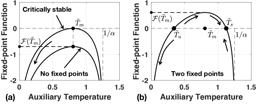
Figure 1: Illustration of fixed point function when there is (a) no fixed point and (b) when there are two fixed points, respectively. The figure is adapted from [12].

Corollary 1

The maxima of $\mathcal{F}(\tilde{T})$ is given by:

$$\mathcal{F}(\tilde{T}_{m})=\ln\beta-\ln\left(\frac{2}{\tilde{T}_{m}}+1\right)e^{-\tilde{T}_{m}}$$

Moreover, equation (9) has two fixed points if the maxima of $\mathcal{F}(\tilde{T})$ is greater than zero. Consequently, (9) has two fixed points if and only if

$$\beta\geq\left(\frac{2}{\tilde{T}_{m}}+1\right)e^{-\tilde{T}_{m}}$$ (12)

where $\tilde{T}_{m}$ depends only on the parameter $\alpha$ and it is defined in (11). Otherwise, it has no solution.

At runtime, the value of $\tilde{T}_{m}$ is computed using (11). Then, the condition for existence of fixed points given in Corollary 1 (Eq. 12) is evaluated. If it is not satisfied, there will be a thermal runaway as presented in Theorem 1 below. In practice, this means that the system will either throttle cores aggressively or perform an emergency shutdown.

III-B2 Stability of the Fixed Points

The behavior of $\tilde{T}$ as a function of $\mathcal{F}(\tilde{T})$ determines the stability of the fixed points. This behavior is summarized using the following lemma in [12].

Lemma 2

The value of $\tilde{T}$ in the temperature iteration increases when $\mathcal{F}(\tilde{T})<0$, and decreases when $\mathcal{F}(\tilde{T})>0$.

This lemma can be used to determine the stability using the sign of $\mathcal{F}(\tilde{T})$. The following theorem in [12] gives the stability of the fixed points using this lemma.

Theorem 1

The stability of the fixed points is as follows:

1. When (10) has no solution, the temperature iteration diverges, i.e., $\tilde{T}\rightarrow 0$ $(T\rightarrow\infty)$, as illustrated in Figure 1. Hence, there is a thermal runaway.

2. When there are two fixed points, $\tilde{T}_{u}\in(0,\tilde{T}_{m})$ is unstable and $\tilde{T}_{s}\in(\tilde{T}_{m},\frac{1}{\alpha})$ is stable.

3. In the latter case, any temperature iteration starting $(0,\tilde{T}_{u})$ diverges, i.e., $\tilde{T}\rightarrow 0$ and $T\rightarrow\infty$ leading to a thermal runaway. However, any temperature iteration starting in $(\tilde{T}_{u},\frac{1}{\alpha})$ converges to the stable fixed point $\tilde{T}_{s}$.

Theorem 1 states that the temperature proceeds along the arrows shown in Figure 1. When $\mathcal{F}(\tilde{T}_{m})<0$, i.e., no fixed point exists, $\tilde{T}$ decreases at each temperature iteration no matter where it starts. This means that $T$ increases in each temperature iteration due to (7). Therefore, there is a thermal runaway as illustrated in Figure 1(a). When $\mathcal{F}(\tilde{T}_{m})>0$, there are two fixed points denoted by $\tilde{T}_{u}$ and $\tilde{T}_{s}$. Iterations that start in the interval $(0,\tilde{T}_{u})$ diverge to $\tilde{T}\rightarrow 0$, since $\mathcal{F}(\tilde{T})<0$ in $(0,\tilde{T}_{u})$. Conversely, temperature iterations with initial points in the interval $(\tilde{T}_{u},\tilde{T}_{s})$ will converge to $\tilde{T}_{s}$, since $\mathcal{F}(\tilde{T})>0$. That is, temperature iterations starting in the interval $(\tilde{T}_{u},\frac{1}{\alpha})$ will also converge to $\tilde{T}_{s}$, as illustrated in Figure 1(b). Therefore, iterations starting in $\tilde{T}_{u}\in(0,\tilde{T}_{m})$ are divergent, while iterations starting in $\tilde{T}_{s}\in(\tilde{T}_{m},\frac{1}{\alpha})$ are convergent.

IV Fixed-Point Analysis for MIMO System

The SISO model in the previous sections allows us to analyze the behavior of thermal hotspots individually. However, in a multiprocessor system there is a close interaction of different resources in the system. As a result of this, activity in one part of the system affects the fixed-point temperatures in other parts of the system. Therefore, it is important to solve the MIMO system in (4) to calculate the fixed-point temperatures. The steady-state equation of the temperature dynamics can be modeled as

$$\mathbf{T^{*}}=\mathbf{A}\mathbf{T^{*}}+\mathbf{B}\mathbf{P^{*}}$$ (13)

where $\mathbf{T^{*}}$ and $\mathbf{P^{*}}$ are the steady-state temperatures and power consumptions, respectively. Define the following function,

$$\mathbf{f(\mathbf{T^{*}})}=(\mathbf{A}-\mathbf{I})\mathbf{T^{*}}+\mathbf{B}\mathbf{P^{*}}.$$ (14)

where $\mathbf{f(\mathbf{T^{*}})}$ is obtained by grouping the temperature terms in (13). $\mathbf{f(\mathbf{T^{*}})}$ is a vector-valued function that depends on $\mathbf{T^{*}}=[T_{1},\ldots,T_{N}]^{T}$ and $\mathbf{P^{*}}=[P_{1},\ldots,P_{M}]^{T}$ satisfying a set of nonlinear equations in terms of $\mathbf{T^{*}}$. This is a nonlinear system of equations due to the exponential temperature terms in $P_{i}$. The standard approach to solving this problem is to find a good initial point and use a root-finding algorithm to solve the nonlinear equations. In this work, we use the Newton’s method [32] to solve the system of equations in (14). The number of iterations required for Newton’s method depends on the initial points. An effective method to find good initial points is to use a reduced-order SISO system as described in [12]. The SISO solution provides fixed points with high accuracy and very low computational cost. Therefore, the SISO model of each hotspot can be used as the initial point in the Newton iterations. The convergence of Newton iterations, i.e., the existence of fixed points, will depend on the system parameters and the power consumption of each of the components. Next, we analyze the region of convergence of the power-temperature dynamics on the Odroid-XU3 board.

IV-A Region of Convergence for Power-Temperature Dynamics

The fixed-point function is given in (14) as

$$\mathbf{f}(\mathbf{T^{*}})=(\mathbf{A}-\mathbf{I})\mathbf{T^{*}}+\mathbf{B}\mathbf{P^{*}}.$$ (15)

We can write the Jacobian matrix of $\mathbf{f}(\mathbf{T^{*}})$ as

$$\mathbf{J}_{\mathbf{f}}(\mathbf{T^{*}})=(\mathbf{A}-\mathbf{I})+\mathbf{B}\mathbf{P^{*}}^{\prime},$$ (16)

where $\mathbf{P^{*}}^{\prime}$ is the derivative of the power consumption values with respect to the temperatures. In each iteration of Newton’s method, the temperature vector step is given by,

$$\Delta\mathbf{T^{*}}_{k}=-\mathbf{J}^{-1}_{\mathbf{f}}(\mathbf{T^{*}}_{k})\mathbf{f}(\mathbf{T^{*}}_{k})$$ (17)

where $k$ denotes the current iteration of Newton’s method. Using $\Delta\mathbf{T^{*}}_{k}$, the temperature vector is updated as,

$$\mathbf{T^{*}}_{k+1}=\mathbf{T^{*}}_{k}-\mathbf{J}^{-1}_{\mathbf{f}}(\mathbf{T^{*}}_{k})\mathbf{f}(\mathbf{T^{*}}_{k}),$$ (18)

where subscripts $k$ and $k+1$ are used to denote temperature in the current iteration and the next iteration, respectively. Using (18), we can define the Newton function $\mathbf{g}(\mathbf{T^{*}}_{k})$ as

$$\mathbf{g}(\mathbf{T^{*}}_{k})=\mathbf{T^{*}}_{k}+\Delta\mathbf{T^{*}}_{k}.$$ (19)

The Newton function gives all the temperatures that will be encountered during the evaluations of Newton’s method. We use this definition of the Newton function to analyze the stability and region of convergence of the power-temperature dynamics of the system. Specifically, the system has a guaranteed convergence to the unique fixed point by Contraction Mapping Theorem (see p.220 in [33]) if the following conditions are satisfied:

• Range of the Newton function is contained in the domain of the function. If the domain of the function is defined as the safe operating limits of the device, this condition ensures that all the temperature vectors given by Newton’s method lie within safe operating limits of the device.

• Norm of the Jacobian of the Newton function $\mathbf{g}(\mathbf{T^{*}}_{k})$ is less than 1.

These conditions will be satisfied for a range of power consumption and system parameters. These bounds can be found by analyzing the properties of $\mathbf{J}^{-1}_{\mathbf{f}}(\mathbf{T^{*}})$ and $\mathbf{f}(\mathbf{T^{*}})$, which is challenging due to the non-linearity. Therefore, in order to evaluate the region of convergence of the system, we analyze whether the previous conditions are satisfied for a range of power consumption values.

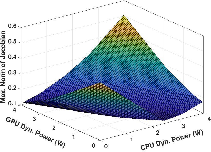
Figure 2: Maximum norm of the derivative of the Newton function when varying the CPU and GPU power consumption.

In order to evaluate the region of convergence of the power-temperature dynamics, we recursively evaluate the MIMO model equations (15) to (19). The system parameters that affect the region of convergence include $\mathbf{A}$, $\mathbf{B}$ matrices and the leakage power parameter of each resource. For a given set of system parameters, the power-temperature dynamics has a guaranteed convergence to a stable and safe fixed point for a range of power consumption and temperature values. The range of temperature for which the processor can operate safely is typically determined by the manufacturer. Therefore, the analysis performed in this section focuses on the range of power consumption for which convergence is guaranteed. As a first step, the nominal values of the system parameters determined from system identification are used to perform the simulations. Then, power consumption of the big cluster and GPU, which are the resources with temperature hotspots in the system, are swept from 0.0024 W to 4 W. We chose this range of power consumption values, since it is the typical power consumption range observed in a wide range of benchmarks. For each power consumption pair, the range of the Newton function $\mathbf{g(\mathbf{T^{*}})}$ and derivative of the Newton function are evaluated over the allowable temperature range of 37^∘C to 120^∘C. Using these results, the range of power consumption values for which the power-temperature dynamics in the system converges to a safe temperature is determined.

In order to have guaranteed convergence, the norm of the derivative must be less than 1 and range of the Newton function must be contained in the domain. As we can see in Figure 2, the maximum norm of the Jacobian is less than 1 for the entire range of power consumption values. However, when the CPU power is greater 3.5 W, the range of the Newton function $\mathbf{g}(\mathbf{T^{*}}_{k})$ is no longer contained in the domain. This means that there exists a temperature trajectory exceeding the maximum safe temperature of the board. Similarly, if the GPU power consumption is greater than 3.5 W, the range of the Newton function is not contained in the domain, as shown in Figure 3. Therefore, we can conclude that the system has guaranteed convergence when the power consumption of the CPU and GPU are in the shaded region shown in Figure 3. We see that the system has guaranteed convergence when the total dynamic power consumption of the CPU and GPU is less than about 3.5 W. This agrees with our experiments on the Odroid-XU3 board where sustained operation at power consumption higher than 3.5 W lead to thermal throttling of the system.

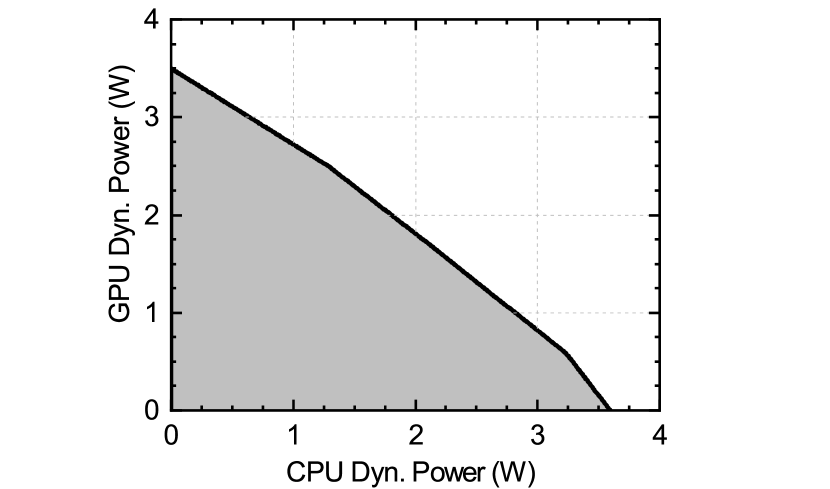
Figure 3: The region of power consumption values for which the range of the Newton function is contained in the domain. The proposed technique guarantees convergence when the total dynamic power consumption of the CPU and GPU is less than about 3.5 W. This result is aligned with our experiments on the Odroid-XU3 board where sustained operation at power consumption higher than 3.5 W lead to thermal throttling of the system.

IV-B Accelerating Newton Iterations

Newton’s method involves the calculation of $\mathbf{J}^{-1}_{\mathbf{f}}(\mathbf{T^{*}}_{k})$ in each iteration. This can be computationally expensive since we have to perform the inversion for multiple Newton iterations every time the fixed points are evaluated. Therefore, we exploit the structure of the temperature dynamics of the experimental platform to speed up the Newton’s method. The Odroid XU3 board consists of a little CPU cluster, a big CPU cluster, main memory and a GPU. Each CPU cluster contains four physical cores. The temperature hotspots in this system include the big cores and the GPU. Using this structure, the fixed-point function can be simplified by separating the temperature-dependent and temperature-independent terms as,

$$\mathbf{f}(\mathbf{T^{*}})=(\mathbf{A}-\mathbf{I})\mathbf{T^{*}}+\mathbf{B}\begin{bmatrix}p_{little}\\ p_{big,1}+p_{big,2}s_{big}\\ p_{mem}\\ p_{gpu,1}+p_{gpu,2}s_{gpu}\end{bmatrix},$$ (20)

where $p_{big,1}$ and $p_{gpu,1}$ are temperature-independent components of the big cluster and GPU, respectively. Temperature-dependent components of only the big cluster and GPU are considered as they have the largest effect on the temperature hotspots. The temperature-dependent components of power are defined as,

$$p_{big,2} =V_{big}\kappa_{1,big}, s_{big} =T_{big}^{2}\exp\Big{(}\frac{-\kappa_{2,big}}{T_{big}}\Big{)},$$

$$p_{gpu,2} =V_{gpu}\kappa_{1,gpu}, s_{gpu} =T_{gpu}^{2}\exp\Big{(}\frac{-\kappa_{2,gpu}}{T_{gpu}}\Big{)}.$$

Similarly, the Jacobian $\mathbf{J}_{\mathbf{f}}(\mathbf{T^{*}})$ can be written as,

$$\mathbf{J}_{\mathbf{f}}(\mathbf{T^{*}})=(\mathbf{A}-\mathbf{I})+p_{big,2}\tilde{s}_{big}b_{1}\begin{bmatrix}0&0&1&0&0\end{bmatrix}\\ +p_{gpu,2}\tilde{s}_{gpu}b_{4}\begin{bmatrix}0&0&0&0&1\end{bmatrix}$$ (21)

where $b_{i}$ denotes the $i$th column of the $\mathbf{B}$ matrix and

$$\tilde{s}_{cpu}= \exp\Big{(}\frac{-\kappa_{2,big}}{T_{big}}\Big{)}(2T_{big}+\kappa_{2,big}),$$

$$\tilde{s}_{gpu}= \exp\Big{(}\frac{-\kappa_{2,gpu}}{T_{gpu}}\Big{)}(2T_{gpu}+\kappa_{2,gpu}).$$ (22)

Since $\tilde{s}_{cpu}$ and $\tilde{s}_{cpu}$ are scalars, (21) can be written as,

$$\begin{split}\mathbf{J}_{\mathbf{f}}(\mathbf{T^{*}})={}&(\mathbf{A}-\mathbf{I})+p_{big,2}b_{1}\tilde{s}_{big}\begin{bmatrix}0&0&1&0&0\end{bmatrix}\\ &+p_{gpu,2}b_{4}\tilde{s}_{gpu}\begin{bmatrix}0&0&0&0&1\end{bmatrix},\end{split}$$

$$\begin{split}={}&(\mathbf{A}-\mathbf{I})+\begin{bmatrix}p_{big,2}b_{1}&p_{gpu,2}b_{4}\end{bmatrix}_{5\times 2}\begin{bmatrix}\tilde{s}_{big}&0\\ 0&\tilde{s}_{gpu}\end{bmatrix}_{2\times 2}\\ &\begin{bmatrix}0&0&1&0&0\\ 0&0&0&0&1\end{bmatrix}_{2\times 5},\end{split}$$

$$\begin{split}={}&(\mathbf{A}-\mathbf{I})\\ &+\begin{bmatrix}p_{big,2}b_{1}&p_{gpu,2}b_{4}\end{bmatrix}_{5\times 2}\begin{bmatrix}\tilde{s}_{big}&0\\ 0&\tilde{s}_{gpu}\end{bmatrix}_{2\times 2}\mathbf{V}_{2\times 5},\end{split}$$

where $\mathbf{V}=\begin{bmatrix}0&0&1&0&0\\ 0&0&0&0&1\end{bmatrix}_{2\times 5}$.

When Newton’s method is used to solve the fixed-point function, the temperature step in each iteration is given by

$$\Delta\mathbf{T^{*}}=-\mathbf{J}^{-1}_{\mathbf{f}}(\mathbf{T^{*}})\mathbf{f}(\mathbf{T^{*}}).$$ (23)

Without changing the value of $\Delta\mathbf{T^{*}}$, we can write

$$\Delta\mathbf{T^{*}}=-((\mathbf{A}-\mathbf{I})^{-1}\mathbf{J}_{\mathbf{f}}(\mathbf{T^{*}}))^{-1}(\mathbf{A}-\mathbf{I})^{-1}\mathbf{f}(\mathbf{T^{*}}).$$ (24)

Now, let $\mathbf{f}_{1}(\mathbf{T^{*}})=(\mathbf{A}-\mathbf{I})^{-1}\mathbf{f}$ and $\tilde{\mathbf{f}}_{1}(\mathbf{T^{*}})=(\mathbf{A}-\mathbf{I})^{-1}\mathbf{J}_{\mathbf{f}}(\mathbf{T^{*}})$. Using (20), $\mathbf{f}_{1}(\mathbf{T^{*}})$ is written as,

$$\mathbf{f}_{1}(\mathbf{T^{*}})=\mathbf{T^{*}}+(\mathbf{A}-\mathbf{I})^{-1}\mathbf{B}\begin{bmatrix}p_{little}\\ p_{big,1}+p_{big,2}s_{big}\\ p_{mem}\\ p_{gpu,1}+p_{gpu,2}s_{gpu}\end{bmatrix}.$$ (25)

Similarly, $\tilde{\mathbf{f}}_{1}(\mathbf{T^{*}})=(\mathbf{A}-\mathbf{I})^{-1}\mathbf{J}_{\mathbf{f}}(\mathbf{T^{*}})$ is written as,

$$\tilde{\mathbf{f}}_{1}(\mathbf{T^{*}})=\mathbf{I}+(\mathbf{A}-\mathbf{I})^{-1}\begin{bmatrix}p_{big,2}b_{1}&p_{gpu,2}b_{4}\end{bmatrix}_{5\times 2}\\ \begin{bmatrix}\tilde{s}_{big}&0\\ 0&\tilde{s}_{gpu}\end{bmatrix}_{2\times 2}V_{2\times 5}.$$ (26)

In order to simplify the notation, we can define matrices $\mathbf{U}$ and $\mathbf{C}$ as,

$$\mathbf{U}={} (\mathbf{A}-\mathbf{I})^{-1}\begin{bmatrix}p_{big,2}b_{1}&p_{gpu,2}b_{4}\end{bmatrix},$$

$$\mathbf{C}={} (\mathbf{A}-\mathbf{I})^{-1}\mathbf{B}\begin{bmatrix}p_{little}&0&0\\ p_{big,1}&p_{big,2}&0\\ p_{mem}&0&0\\ p_{gpu,1}&0&p_{gpu,2}\end{bmatrix}.$$ (27)

Using this notation, (25) can be rewritten as,

$${\mathbf{f}}_{1}(\mathbf{T^{*}})=\mathbf{T^{*}}+c_{1}+\begin{bmatrix}c_{2}&c_{3}\end{bmatrix}\begin{bmatrix}s_{big}\\ s_{gpu}\end{bmatrix}.$$ (28)

where $c_{i}$ denotes the $i$th column of $\mathbf{C}$. Similarly, (26) can be rewritten as,

$$\tilde{\mathbf{f}}_{1}(\mathbf{T^{*}})=\mathbf{I}+\mathbf{U}\begin{bmatrix}\tilde{s}_{big}&0\\ 0&\tilde{s}_{gpu}\end{bmatrix}\mathbf{V}.$$ (29)

In order to calculate the step size $\Delta\mathbf{T^{*}}$, the inverse of $\tilde{f}_{1}$ has to be evaluated at each step. The inverse can be easily calculated using the matrix inversion lemma [34] on (29). Consequently, the inverse of $\tilde{\mathbf{f}}_{1}(\mathbf{T^{*}})$ in (29) is written as

$$\tilde{\mathbf{f}}^{-1}_{1}(\mathbf{T^{*}})=\mathbf{I}-\mathbf{U}\Bigg{(}\begin{bmatrix}1/\tilde{s}_{big}&0\\ 0&1/\tilde{s}_{gpu}\end{bmatrix}+\mathbf{VU}\Bigg{)}^{-1}\mathbf{V}.$$ (30)

This simplification reduces to an inversion of a $2\times 2$ matrix, which can be achieved with simple algebraic operations. The evaluation of $\mathbf{U}$ requires computing $(\mathbf{A}-\mathbf{I})^{-1}$, which can be computed offline and stored in the system.

Using (25) and (29), the temperature step can be written as,

$$\Delta{\mathbf{T^{*}}}=-\tilde{\mathbf{f}}^{-1}_{1}(\mathbf{T^{*}})*{\mathbf{f}}_{1}(\mathbf{T^{*}}).$$ (31)

It can be seen that the calculation of $\Delta{\mathbf{T^{*}}}$ consists of only a matrix multiplication and the matrix inversion is eliminated. This translates to a signification reduction in the computational overhead of the Newton iterations. A detailed analysis of the execution time savings is presented in Section VI-F.

V Temperature Control using Fixed Points

One of the primary applications of the fixed-point prediction is to enable better dynamic thermal and power management (DTPM) algorithms. State-of-the-art DTPM algorithms typically throttle the entire system when a thermal violation is detected. This causes a performance loss for all the applications running in the system. Moreover, DTPM algorithms start throttling only after the temperature violates a threshold, which is not desirable. In contrast to these approaches, the fixed-point prediction can be used to make better DTPM decisions. It provides an estimate of the long-term thermal behavior of the system. This estimate can be used to determine the possibility of a thermal violation in the future. In addition to the fixed-point prediction, the time to reach the fixed-point estimate [12] gives a lower bound on the time at which the fixed point is attained.

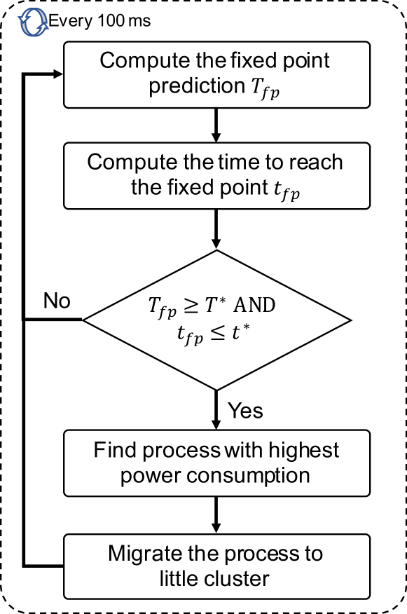
Figure 4: Overview of the proposed control algorithm.

Estimates of the fixed point and the time to reach can be used to design a simple control algorithm, as shown in Figure 4. The algorithm starts by computing the fixed point $T_{fp}$, followed by the time to reach the fixed point $t_{fp}$. A thermal violation is imminent if $T_{fp}$ is greater than a specified thermal limit $T^{*}$ and $t_{fp}$ is less than a specified time limit $t^{*}$. In these cases, the algorithm finds the process with the highest power consumption. This is achieved by monitoring the utilization of active processes over a one-second window and choosing the process with the highest utilization. We use a one-second window to ensure that momentary peaks in the power consumption are filtered out. Then, it moves the process to the low-power processors in the system. Once the process is moved to the low-power processor it is kept there for a fixed period (one control interval in our implementation). After the period is over, the default scheduling algorithms on the device are free to move the process back to the big core as a function of its processing requirements. This ensures that the process is not starved of computing resources once the temperature of the device is within safe limits. In addition to moving the process to low-power processors, we can also reduce the frequency of the core it is running on such that processes running on other cores are not penalized. However, the Odroid XU3 board used in our experimental evaluations allows control of frequency at the granularity of clusters (A15 or A7). Due to this limitation of the hardware platform, the control algorithm migrates the process with the highest power consumption to the low-power processors.

We invoke the control algorithm every 100 ms at runtime. We choose a 100 ms interval since the frequency management governors in typical smartphone operating systems, e. g. Android, apply frequency control decisions with this period. That is, the frequency governors present in the system evaluate the utilization of resources and the workload every 100 ms. Based on this evaluation, new frequencies for each resource are set. Therefore, the 100 ms interval for the invocation of the control algorithm allows us to capture these dynamic changes in the system (e.g. a new task starts to consume high power and raises the temperature). We note that the execution interval of the control algorithm can be changed dynamically as a function of the rate at which new processes are launched. For example, if new applications are being launched more frequently than every 100 ms we can decrease the execution interval of the control algorithm at the expense of increased runtime overhead.

The main benefit of our algorithm is that it only penalizes the processes that lead to thermal violations. All other processes running in the system are not penalized; hence, they can continue to operate with maximum performance. Furthermore, processes with real-time requirements can register themselves, so that they are not penalized by the algorithm. An illustration of the proposed algorithm is presented in the experiments.

One of the most important components of the control algorithm is the accurate prediction of the time to reach the fixed point. The approach proposed in [12] uses two temperature readings separated by a fixed amount of time to predict the time to reach the fixed point. While this approach provides a prediction with a very low computational overhead, the error in the prediction can be high. Therefore, in this paper, we use an improved approach that utilizes a larger number of samples to determine $t_{fp}$. Specifically, we maintain a vector that contains the envelope of the temperature measurements. The envelope of the temperature at any time step $k$ can be expressed as:

$$T_{u}[kT_{s}]=\max\{T[(k-M)T_{s}],T[(k-M+1)T_{s}],\dots,T[kT_{s}]\}$$ (32)

where $T_{u}[k]$ is the envelope temperature at time $kT_{s}$ using a sampling period of $T_{s}$, $M$ is the size of the window over which we take the maximum, $T[(k-M)T_{s}]$ is the temperature at time $(k-M)T_{s}$ and $T[kT_{s}]$ is the temperature at time $kT_{s}$. We take the maximum over a window to ensure that momentary spikes in the temperature are filtered out. An example of the temperature envelope is provided in Figure 7 in the experimental evaluations. The envelope data is then used to fit a first-order exponential model given by:

$$T[kT_{s}]=T_{u,init}+(T_{fix}-T_{u,init})(1-e^{-\frac{kT_{s}}{\tau}})$$ (33)

where $T_{u,init}$ is the initial upper envelope temperature, $T_{fix}$ is the fixed-point prediction and $\tau$ is the time constant for the first-order model. We use a nonlinear curve fitting tool to fit the upper envelope temperature data to the model in (33). The quality of the fit depends on the number of data points used in the curve fitting. A larger number of data points ensures a fit with lower error. However, the system needs to wait for a longer period of time to allow the accumulation of upper envelope temperature. In contrast, fewer data points can provide a faster estimation of the time to fixed point, albeit with a higher error. We explore this trade-off to determine the optimal number of data points, as shown in Section VI-D. In addition to the first-order exponential model, we evaluated a second-order model to estimate the time to the fixed point. However, we observed that the first time constant dominates the second time constant, implying that the model is strongly first order. Therefore, we use a first-order model in our experimental evaluations.

VI Experimental Evaluation

VI-A Experimental Setup

We perform evaluations of the proposed fixed-point prediction scheme using the Odroid-XU3 board. The Odroid-XU3 board uses the Samsung Exynos 5422 system-on-chip [14] that integrates four Cortex-A15 (big) cores, four Cortex-A7 (little) cores, and a Mali T628 GPU. It also includes thermal sensors to measure the temperature of each big core and the GPU. Furthermore, the platform provides current sensors that allow us to obtain the power consumption of the little cluster, big cluster, main memory, and the GPU at runtime. The board is installed with Android 7.1 running Linux kernel 3.10.9. We invoke the fixed-point framework and the control algorithm every 100 ms, along with the default frequency governors. The proposed approach is evaluated on Android benchmarks, such as 3DMark and Nenamark3. We choose 3DMark and Nenamark3 benchmarks because they are able to give standard metrics to measure the performance of various devices and algorithms. Both benchmarks run a series of tests on the device and report a metric at the end. Hence, we can compare the performance of the Odroid-XU3 board with and without our proposed approach.

VI-B Parameter Estimation and Accuracy Evaluation

The thermal fixed-point analysis presented in this paper does not assume any specific values for the system parameters. However, in order to validate the fixed-point analysis, system parameters have to be characterized. Specifically, we characterize the system parameters (e.g., matrices $\mathbf{A}$, $\mathbf{B}$, and the leakage power) for the experimental platform. We use the ssest function in the system identification of MATLAB [35] to the thermal model matrices $\mathbf{A}$ and $\mathbf{B}$. From the system identification, we observe that both $\mathbf{A}$ and $\mathbf{B}$ matrices are full rank. Similarly, nonlinear curve fitting is used to estimate the leakage power parameters for the big cluster and GPU. Further details on the methodology used to characterize the parameters are presented in [12] and [21].

Accuracy of Fixed-Point Predictions: The effectiveness of the proposed control algorithm depends on the accuracy of the fixed-point predictions. Therefore, we perform a detailed accuracy evaluation with ten compute-intensive benchmarks. Across the ten benchmarks, the highest error observed is 5.8$\degree$C which translates to a 6% error. On average, the proposed analysis predicts the fixed point with about 3$\degree$C (5%) error. For more details of the accuracy, such as the error for each benchmark, please refer to [12].

VI-C Power-Temperature Trajectory for MIMO Iterations

In this section, the fixed-point prediction is compared against the measured power-temperature trajectory for the GPU. In order to get an accurate experimental fixed point, the total power consumption of the device is kept at a constant level of about 1.18 W. Then, the fixed point of the GPU is calculated using the measured power consumption values, as shown using a red diamond in Figure 5. It is seen that the experimental fixed-point value closely matches the predicted fixed point. In addition to the prediction, simulations using different initial values of temperature and power consumption are performed. The simulations use the thermal and leakage power models to update the temperature and leakage power iteratively. We see that all the simulated trajectories converge to the predicted fixed point. Moreover, the measured power-temperature trajectory closely follows the simulated trajectory. This demonstrates that the thermal and power models identified closely match the dynamics of the device.

The temperature trajectory in Figure 5 can also be used to estimate CPU to environment thermal resistance of the device. The thermal resistance is defined as:

$$\theta=\frac{\Delta T}{P}$$ (34)

where $\theta$ is the thermal resistance, $\Delta T$ is the temperature differential, and $P$ is the power consumption. From the figure, we see that $\Delta T$ is 23$\degree$C while the power consumption $P$ is set as 1.18 W. Using this the thermal resistance $\theta$ is obtained as 19.48$\degree$C/W. We can also obtain the thermal resistance using the SISO model in (5). Specifically, we can write the thermal resistance as:

$$\theta=\frac{b}{1-a}.$$ (35)

Using the parameters obtained using system identification for $a=0.9994$ and $b=0.0121$, we can calculate the thermal resistance as 20.1$\degree$C/W, which is in close agreement to the value obtained experimentally. This shows that the proposed system identification methodology is able to accurately capture the thermal dynamics of the system. We note that more detailed models for the thermal resistance can be obtained if the details about the location of temperature sensors and chip packaging are publicly available. However, in the absence of these details we use system identification to gain insights into the thermal dynamics of the system.

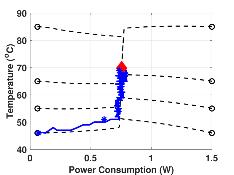
Figure 5: Power trajectory of the GPU when the total power consumption of the device is held constant at about 1.18 W

VI-D Time to Reach the Fixed Point

Accurate estimation of the time to reach the fixed point is an important component of the proposed control algorithm. Underestimation of the time to fixed point can lead to thermal issues, while overestimation leads to performance loss due to aggressive throttling. As explained in Section V, the accuracy of the time to fixed-point estimation depends on the number of data points used to fit the first-order model. Therefore, we evaluate the accuracy of the time to fixed-point estimation as a function of the number of data points used for the estimation. We can vary the number of samples used in the fitting by controlling the delay in fitting or by controlling the sampling rate of the temperature measurements. Figure 6 shows the error in the time to the fixed point as we vary the sampling rate and the delay in fitting. We observe that using temperature measurements in a shorter window and a lower sampling rate results in a higher error. As we increase the length of the window and the sampling rate, the error progressively reduces. We also observe that length of the window is more important than the sampling rate of the temperature measurements. For instance, using a 200 s window at a sampling rate of 10 Hz results in an error of only 5%, while shorter windows result in a higher error. A 200 s window is acceptable to obtain an accurate estimation of the time to fixed point as it takes more than 500 s for the system to attain steady state.

Figure 7 shows the comparison of the measured temperature, upper envelope temperature, and the first-order fit, for the Vortex workload in the SPEC benchmark suite, using the temperature measurements in the first 200 s. We see that the first-order fit closely follows the upper envelope temperature. Moreover, the time at which the first-order fit reaches the steady state differs from the actual time by about 10%. This error is acceptable since the fit is repeated every second. Therefore, as more data becomes available, the error decreases continuously. As a result of this, the control algorithm has the most up-to-date estimation of the time to the fixed point.

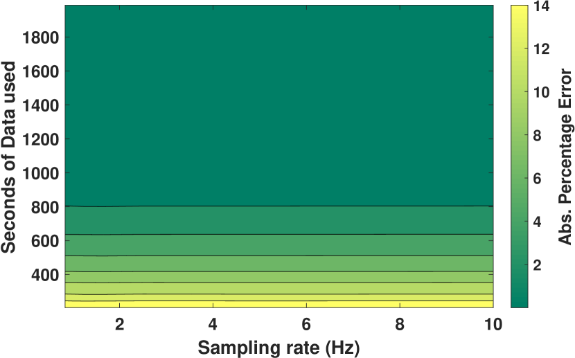
Figure 6: Comparison of prediction of time to the fixed point.

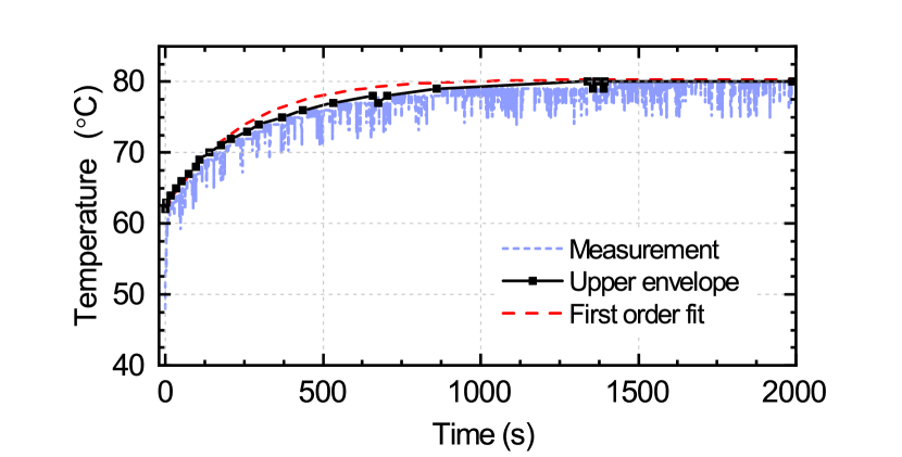
Figure 7: Comparison of temperature measurement, upper envelope of the temperature, and our first-order fit.

VI-E Application Control Using Fixed-Point predictions

This section presents an illustration of the control algorithm using fixed-point predictions. We run a real-time GPU benchmark along with a computationally intensive task in the background to evaluate the effectiveness of the control algorithm. The default policy is to use the thermal management algorithm in the Linux kernel version 3.10.9. Specifically, it uses fixed temperature thresholds and the ARM intelligent power allocation (IPA) algorithm to control the temperature [36]. ARM IPA uses a proportional-integral-derivative feedback controller (PID) to manage the temperature of the device. The IPA policy has a control temperature set at the time of its initialization. At runtime, it compares the control temperature to the maximum temperature observed in the system. Then, it finds the error between the control temperature and measured maximum temperature. Based on this error term, the IPA algorithm sets the frequency of each computing resource. We use the IPA algorithm as the baseline in our comparisons. The on-board fan is disabled during these evaluations since it is not a viable option for mobile platforms.

TABLE II: Maximum temperature of the system when using the default policy, DTPM, and the proposed control algorithm, respectively. A temperature violation occurs when the maximum temperature is higher than 85$\degree$C

Scenario	Number of thermal violations
3DMark (Baseline)	19
3DMark + BML (Baseline)	1294
3DMark + BML (Proposed approach)	176

TABLE III: Comparison of performance of three applications with proposed control

Test	App. Alone	App. + BML	App. + BML with Proposed Control
3DMark GT1	97 fps	86 fps	93 fps
3DMark GT2	51 fps	49 fps	52 fps
Nenamark3	3.5 levels	3.4 levels	3.5 levels

3D Mark alone: We start by running the 3DMark benchmark alone without introducing any background applications. Specifically, we run graphics test 1 (GT1) and graphics test 2 (GT2) benchmarks in the 3DMark application. We obtain an upper bound on the performance with this experiment. This experiment also gives us the baseline temperature profile, as shown in Table II. A thermal violation occurs whenever the maximum temperature is greater than 85$\degree$C, the temperature at which the default governor starts throttling the system. The first row of Table II shows that there are 19 thermal violations when running 3DMark alone. We also analyze the power consumption of each SoC component when running the 3DMark application in Figure 8. The GPU consumes about 42% of the total power since 3DMark is a GPU-intensive application. This is followed by the big cluster that consumes 38% of the power to perform computational parts of 3DMark.

3D Mark + BML (IPA): In the second part of the evaluation, we re-run the 3DMark benchmark along with the Basicmath Large (BML) application [37] in the background. BML is a CPU-intensive application that performs mathematical computations. As a result, it leads to an increase in the big core power consumption, which causes the total power consumption to increase to 3.65 W. The increase in the big core power consumption also increases its contribution to the total power from 38% to 60%, as shown in Figure 8. The higher power consumption causes the temperature to increase quickly beyond 85$\degree$C. Indeed, the number of thermal violations increases to 1294. As a result of this increase, the default IPA thermal governor starts to reduce the frequency of all the resources in the system. This leads to an undesirable drop in performance of GT1 and GT2, as shown in the third column of Table III. Specifically, the frame rate of GT1 decreases from 97 to 86 frames per second (fps), while the frame rate of GT2 decreases from 51 fps to 49 fps.

Proposed Control: Finally, we apply the proposed control algorithm when both 3D Mark and BML are running on the board. As expected, BML causes the power consumption and the temperature to rise. The proposed algorithm keeps track of the increase in the power consumption and updates its estimates of the fixed point continuously. As soon as it detects that the thermal limit will be breached in the near future, it migrates BML to the little cluster to reduce the number of thermal violations. The migration successfully reduces the number violations to 176, as shown in the third row of Table II. The migration also leads to a reduction of the big core power contribution from 60% to 42%, as shown in Figure 8. Moreover, the migration of BML to the little cluster causes its power consumption to increase from 7% to 16% of the total power. The migration effectively throttles BML with minimal performance loss for the 3DMark application, as seen in last column of Table III.

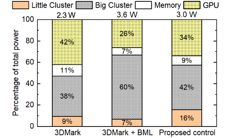
Figure 8: Power consumption distribution of 3DMark.

We repeat the same with the Nenamark3 benchmark in order to evaluate the control algorithm on a benchmark with different characteristics. The Nenamark3 benchmark measures the number of levels the platform can run at a given frame rate. Once the frame rate drops below the reference level, the benchmark terminates and reports the number of levels completed. The last row of Table III summarizes the performance obtained for the Nenamark3 benchmark under the three scenarios. As expected, the performance drops when we run BML along with Nenamark3. In contrast, the proposed control algorithm recovers the performance back to the baseline level. Furthermore, the power consumption follows a trend similar to that of 3DMark, as shown in Figure 9. In summary, the control algorithm effectively detects and migrates the power-hungry applications without affecting the performance of the foreground application.

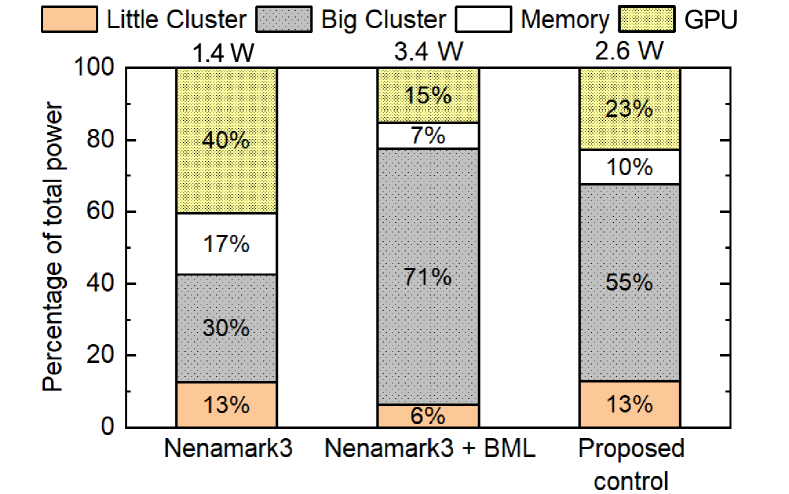
Figure 9: Power consumption distribution for the Nenamark3 benchmark.

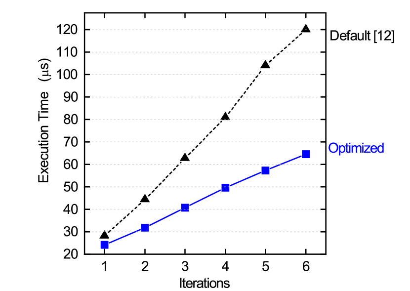
Figure 10: Comparison of the execution time of Newton’s method using the default implementation [12] and the proposed optimized implementation.

Implementation Overhead of Proposed Control: The implementation overhead of the proposed algorithm consists of two parts. The first part involves the evaluation of the fixed points by performing Newton’s method iterations. With our accelerated approach, the computation of the fixed points with six Newton iterations takes about 63 $\mu$s, as detailed in the next section. This computation has to be performed every 100 ms i.e. with every invocation of the control algorithm. The second part of the overhead is incurred when we find the process with the highest power consumption. This part takes about 1 s since we profile the utilization of all processes in the system in a 1 s window. A 1 s window is needed to ensure that momentary peaks in the power consumption can be filtered out. This overhead is not significant since it is invoked infrequently, i.e. only when a thermal violation is predicted. Furthermore, we can reduce the 1 s overhead by running a background task that keeps track of the process with the highest power consumption. In summary, the control algorithm takes only about 63 $\mu$s during normal course of execution, which is less than 0.1% of the 100 ms interval.

VI-F Effect of Accelerated Fixed-Point Computation

The runtime nature of the fixed-point computation necessitates fast and efficient implementation of the fixed-point iterations. Therefore, this section compares the implementation overheads of Newton’s method with and without the proposed optimization. The default implementation of Newton’s method takes about 27 $\mu$s for a single iteration and increases linearly with increasing iterations, as shown in Figure 10. The optimized method, on the other hand, takes about 24 $\mu$s for one iteration and increases at a much lower rate than the default implementation. Overall, we achieve speed up of about 1.8$\times$ when compared to the default implementation.

VII Conclusion

This paper presented a theoretical analysis of the temperature dynamics in multiprocessor systems. We first solved the system of MIMO equations to find the temperature fixed points in the system. Then, we experimentally derived the region of convergence of the CPU-GPU dynamics. Finally, we utilized a control algorithm to manage the temperature of the system without sacrificing the performance. We demonstrated the control algorithm on the Exynos 5422 system on a chip.

Even though we focused our analysis on mobile systems, it can be applied to other low-power devices such as wearables. This can be achieved by modeling the dynamics of these systems and then using the MIMO solution presented in this work. The analysis can be used to improve the thermal behavior in future processors. In particular, the fixed-point analysis can be used to detect power attacks in the system by detecting processes that lead to a high steady-state temperature.

Acknowledgements: This work was supported partially by Semiconductor Research Corporation (SRC) task 2721.001 and National Science Foundation grant CNS-1526562.

Ganapati Bhat received his B.Tech degree in Electronics and Communication from Indian Institute of Technology (ISM), Dhanbad, India in 2012. From 2012-2014, he worked as a software engineer at Samsung Research and Development Institute, Bangalore, India. He is currently a PhD candidate in Computer Engineering at the School of Electrical, Computer and Energy Engineering, Arizona State University. His research interests include energy optimization in computing systems, dynamic thermal and power management, and energy management for wearable systems.

Dr. Gumussoy is a research scientist at Autonomous Systems & Control group at Siemens Corporate Technology in Princeton, NJ. His general research interests are learning, control, identification, optimization and scientific computing with particular focus on reinforcement learning, optimal-adaptive control, frequency domain system identification, time-delay systems and their numerical implementations. He serves as an Associate Editor in IEEE Transactions on Control Systems Technology and IEEE Conference Editorial Board. Dr. Gumussoy received his B.S. degrees in Electrical & Electronics Engineering and Mathematics from Middle East Technical University at Turkey in 1999 and M.S., Ph.D. degrees in Electrical and Computer Engineering from The Ohio State University at USA in 2001 and 2004. He worked as a system engineer in defense industry (2005-2007) and he was a postdoctoral associate in Computer Science Department at University of Leuven (2008-2011). He was a principal control system engineer in Controls & Identification Team at MathWorks where his contributions ranges from state-of-the-art numerical algorithms to comprehensive analysis & design tools in Control System, Robust Control, System Identification and Reinforcement Learning Toolboxes.

Umit Y. Ogras received his Ph.D. degree in Electrical and Computer Engineering from Carnegie Mellon University, Pittsburgh, PA, in 2007. From 2008 to 2013, he worked as a Research Scientist at the Strategic CAD Laboratories, Intel Corporation. He is currently an Associate Professor at the School of Electrical, Computer and Energy Engineering. Recognitions Dr. Ogras has received include Strategic CAD Labs Research Award, 2012 IEEE Donald O. Pederson Transactions on CAD Best Paper Award, 2011 IEEE VLSI Transactions Best Paper Award and 2008 EDAA Outstanding PhD. Dissertation Award. His research interests include digital system design, embedded systems, multicore architecture and electronic design automation with particular emphasis on multiprocessor systems-on-chip (MPSoC).

References

- [1] W. Huang, S. Ghosh, S. Velusamy, K. Sankaranarayanan, K. Skadron, and M. R. Stan, “HotSpot: A Compact Thermal Modeling Methodology for Early-Stage VLSI Design,” IEEE Trans. Very Large Scale Integr. (VLSI) Syst., vol. 14, no. 5, pp. 501–513, 2006.
- [2] B. Egilmez, G. Memik, S. Ogrenci-Memik, and O. Ergin, “User-Specific Skin Temperature-Aware DVFS for Smartphones,” in Proc. 2015 Design, Autom. & Test in Europe Conf. & Exhibition, 2015, pp. 1217–1220.
- [3] R. Kumar, D. M. Tullsen, N. P. Jouppi, and P. Ranganathan, “Heterogeneous Chip Multiprocessors,” Computer, vol. 38, no. 11, pp. 32–38, 2005.
- [4] Samsung Electronics Co. (2016) Samsung Expands Recall to All Galaxy Note7 Devices. http://www.samsung.com/us/note7recall/ Accessed 07/14/2017.
- [5] A. Kumar, L. Shang, L.-S. Peh, and N. K. Jha, “System-Level Dynamic Thermal Management for High-Performance Microprocessors,” IEEE Trans. Comput.-Aided Design of Integr. Circuits Syst., vol. 27, no. 1, pp. 96–108, 2008.
- [6] V. Pallipadi and A. Starikovskiy, “The Ondemand Governor,” in Proc. of the Linux Symp., vol. 2, 2006, pp. 215–230.
- [7] S. Pagani, H. Khdr, J.-J. Chen, M. Shafique, M. Li, and J. Henkel, “Thermal Safe Power (TSP): Efficient Power Budgeting for Heterogeneous Manycore Systems in Dark Silicon,” IEEE Trans. Comput., vol. 66, no. 1, pp. 147–162, 2017.
- [8] A. Vassighi and M. Sachdev, “Thermal Runaway in Integrated Circuits,” IEEE Trans. Device Mater. Rel., vol. 6, no. 2, pp. 300–305, 2006.
- [9] W. Liao and L. He, “Coupled Power and Thermal Simulation with Active Cooling,” in Int. Workshop on Power-Aware Comput. Syst., 2003, pp. 148–163.
- [10] S. Sharifi, D. Krishnaswamy, and T. S. Rosing, “PROMETHEUS: A Proactive Method for Thermal Management of Heterogeneous MPSoCs,” IEEE Trans. Comput.-Aided Design Integr. Circuits Syst., pp. 1110–1123, 2013.
- [11] K. Roy, S. Mukhopadhyay, and H. Mahmoodi-Meimand, “Leakage Current Mechanisms and Leakage Reduction Techniques in Deep-Submicrometer CMOS Circuits,” Proc. of the IEEE, vol. 91, no. 2, pp. 305–327, 2003.
- [12] G. Bhat, S. Gumussoy, and U. Y. Ogras, “Power-Temperature Stability and Safety Analysis for Multiprocessor Systems,” ACM Trans. Embed. Comput. Syst., vol. 16, no. 5s, pp. 145:1–145:19, 2017.
- [13] O. Sahin and A. K. Coskun, “QScale: Thermally-Efficient QoS Management on Heterogeneous Mobile Platforms,” in Proc. Int. Conf. on Comput.-Aided Design, 2016, pp. 125:1–125:8.
- [14] Hardkernel, “ODROID-XU3,” https://wiki.odroid.com/old_product/odroid-xu3/odroid-xu3 Accessed 24 Nov. 2018, 2014.
- [15] P. Li, L. T. Pileggi, M. Asheghi, and R. Chandra, “Efficient Full-Chip Thermal Modeling and Analysis,” in Proc. Int. Conf. on Comput.-Aided Design, 2004, pp. 319–326.
- [16] Y. Zhan and S. S. Sapatnekar, “A High Efficiency Full-Chip Thermal Simulation Algorithm,” in Proc. Int. Conf. on Comput.-Aided Design, 2005, pp. 635–638.
- [17] F. Beneventi, A. Bartolini, A. Tilli, and L. Benini, “An Effective Gray-Box Identification Procedure for Multicore Thermal Modeling,” IEEE Trans. Comput., vol. 63, no. 5, pp. 1097–1110, 2014.
- [18] U. Y. Ogras, R. Marculescu, D. Marculescu, and E. G. Jung, “Design and Management of Voltage-Frequency Island Partitioned Networks-on-Chip,” IEEE Trans. on Very Large Scale Integration Systems, vol. 17, no. 3, pp. 330–341, 2009.
- [19] P. Bogdan, S. Garg, and U. Y. Ogras, “Energy-efficient computing from systems-on-chip to micro-server and data centers,” in Intl. Green and Sustainable Computing Conference (IGSC), 2015, pp. 1–6.
- [20] G. Bhat, S. Gumussoy, and U. Y. Ogras, “Power and thermal analysis of commercial mobile platforms: Experiments and case studies,” in 2019 Design, Automation & Test in Europe Conference & Exhibition (DATE). IEEE, 2019, pp. 144–149.
- [21] G. Bhat, G. Singla, A. K. Unver, and U. Y. Ogras, “Algorithmic Optimization of Thermal and Power Management for Heterogeneous Mobile Platforms,” IEEE Trans. Very Large Scale Integr. (VLSI) Syst., vol. 26, no. 3, pp. 544–557, 2018.
- [22] R. Cochran and S. Reda, “Thermal Prediction and Adaptive Control Through Workload Phase Detection,” ACM Trans. Des. Autom. of Electron. Syst., vol. 18, no. 1, pp. 7:1–7:19, 2013.
- [23] G. Singla, G. Kaur, A. K. Unver, and U. Y. Ogras, “Predictive Dynamic Thermal and Power Management for Heterogeneous Mobile Platforms,” in Proc. 2015 Design, Autom. & Test in Europe Conf. & Exhibition, 2015, pp. 960–965.
- [24] K. Rao, W. Song, S. Yalamanchili, and Y. Wardi, “Temperature Regulation in Multicore Processors Using Adjustable-Gain Integral Controllers,” in Proc. IEEE Conf. on Control Appl. (CCA), 2015, pp. 810–815.
- [25] F. Zanini, D. Atienza, and G. De Micheli, “A Control Theory Approach for Thermal Balancing of MPSoC,” in Proc. Asia and South Pacific Design Autom. Conf., 2009, pp. 37–42.
- [26] A. Leva, F. Terraneo, I. Giacomello, and W. Fornaciari, “Event-Based Power/Performance-Aware Thermal Management for High-Density Microprocessors,” IEEE Trans. Control Syst. Tech., vol. 26, no. 2, pp. 535–550, 2018.
- [27] A. Mutapcic, S. Boyd, S. Murali, D. Atienza, G. De Micheli, and R. Gupta, “Processor Speed Control With Thermal Constraints,” IEEE Trans. Circuits and Syst. I: Regular Papers, vol. 56, no. 9, pp. 1994–2008, 2009.
- [28] S. Heo, K. Barr, and K. Asanović, “Reducing Power Density through Activity Migration,” in Proc. 2003 Int. Symp. on Low Power Electron. and Design, 2003, pp. 217–222.
- [29] P. Dadvar and K. Skadron, “Potential Thermal Security Risks,” in 21st IEEE Semicond. Thermal Meas. & Management Symp., 2005, pp. 229–234.
- [30] J. Hasan, A. Jalote, T. Vijaykumar, and C. E. Brodley, “Heat Stroke: Power-Density-Based Denial of Service in SMT,” in 11th Int. Symp. on High-Performance Computer Arch., 2005, pp. 166–177.
- [31] J. Kong, J. K. John, E.-Y. Chung, S. W. Chung, and J. Hu, “On the Thermal Attack in Instruction Caches,” IEEE Trans. Depend. and Sec. Comput., vol. 7, no. 2, pp. 217–223, 2010.
- [32] K. E. Atkinson, An Introduction to Numerical Analysis. John Wiley & Sons, 2008.
- [33] W. Rudin, Principles of Mathematical Analysis, 3rd ed. McGraw-Hill, New York, 1976.
- [34] C. D. Meyer, Matrix Analysis and Applied Linear Algebra. SIAM, 2000, vol. 71.
- [35] Mathworks. (2018) System Identification Toolbox. https://www.mathworks.com/products/sysid.html Accessed 25 Jan. 2019.
- [36] X. Wang. (2015) Intelligent Power Allocation. http://infocenter.arm.com/help/topic/com.arm.doc.dto0052a/DTO0052A_intelligent_power_allocation_white_paper.pdf, Accessed 4 Dec. 2018.
- [37] M. R. Guthaus, J. S. Ringenberg, D. Ernst, T. M. Austin, T. Mudge, and R. B. Brown, “Mibench: A Free, Commercially Representative Embedded Benchmark Suite,” in Proc. Int. Workshop on Workload Char., 2001, pp. 3–14.