Partial stabilization of nonholonomic systems
with application to multi-agent coordination

Abstract

This paper focuses on the problem of constructing time-varying feedback laws that asymptotically stabilize a given part of the state variables for nonlinear control-affine systems. It is assumed that the class of systems under consideration satisfies nonlinear controllability conditions with respect to the stabilizable variables. Under these assumptions, a time-periodic feedback control is constructed explicitly by using the inversion of the matrix composed of the control vector fields and their Lie brackets. The proposed control design scheme is applied to solving the leader-following problem for nonlinear multi-agent systems. These results are illustrated with two examples of nonholonomic control problems: the partial stabilization of a rolling disc and the leader-following task for two unicycles.

1 Introduction

The development of control algorithms for nonholonomic mechanical systems attracts attention of many researchers because of numerous engineering applications and significant mathematical challenges. A principal challenge in the stabilization of nonholonomic systems is caused by their underactuated structure and essentially nonlinear dynamical properties. However, it should be noted that the requirement of asymptotic stability is redundant in many applied problems, while only the stability with respect to some part of the state variables characterizes the desired behavior of the closed-loop system. For example, such partial stability problems arise from the single axis stabilization of satellites [1, 2], tracking tasks for robotic manipulators with redundant kinematics [3, 4, 5], multi-agent coordination and synchronization tasks.

The stability property with respect to a part of variables was first rigorously introduced by A. M. Lyapunov and further studied, e.g., in [1, 6, 7, 8, 9, 10, 11]. A detailed survey of partial stability results can be found in [12]. Despite significant progress in this area, there are only a few results on the partial stabilization of nonholonomic systems. In particular, the paper [6] examined the relation between partial stability and stability with respect to all variables for nonholonomic mechanical systems and proposed partial stability conditions. A partial stabilization problem for Lagrangian systems has been considered in [13, 14]. Finite-time partial stabilization problem for chained-form and cascade systems has been studied, e.g., in [15, 16]. A more general class of nonlinear control system has been analyzed in [17, 9]. The proposed sufficient partial stability conditions rely on the assumption that the system admits certain Lyapunov-like function, whose time derivative is negative definite with respect to a given part of variables. However, the problem of partial stabilization remains open for general nonholonomic systems, for which the required Lyapunov-like function cannot be effectively constructed.

In [18], we have proposed practical partial asymptotic stability conditions for control-affine systems, whose averaged system has partially asymptotically stable equilibrium. The present paper addresses the problem of explicit construction of partially stabilizing feedback laws for nonlinear control-affine systems, whose vector fields satisfy certain Lie algebra rank condition. We will propose a family of time-periodic feedback laws for partial stabilization of such systems and apply the obtained results to nonlinear multi-agent systems. Note that, although there exist numerous results on multi-agent coordination (see, e.g., [19, 20] for a survey), the development of feedback control algorithms for nonholonomic agents has been addressed so far for specific systems only, such as kinematic or dynamic unicycle models [21, 22, 23, 24, 25, 26, 27, 28, 29, 30], chained-form systems [31], and manipulators [32, 33, 34].

The contribution of this paper is twofold. First, we introduce a novel approach for partial stabilization of nonlinear controllable systems by means of time-varying feedback laws. Unlike other results on partial stabilization of nonholonomic systems, our controllers ensure exponential convergence of the trajectories (see Section 2.B). Second, we adapt these control strategies for the leader-following problem in Section 2.C. The stability proof is presented in Section 3, and the efficiency of the proposed controllers is illustrated by numerical simulations in Section 4.

Basic notations. Throughout this paper, we will use the following notations:

$0_{n}$, $0_{m\times n}$ – $n$-dimensional zero column vector and $m\times n$-dimensional zero matrix, respectively;

$1_{n}$ – $n$-dimensional column vector with all entries being equal to 1;

$I_{m\times n}$ – $m\times n$-dimensional matrix with entries $I_{ii}=1$ and $I_{ij}=0$ whenever $i\neq j$ ($i=\overline{1,m}$, $j=\overline{1,n}$);

$\delta_{ij}$ – Kronecker delta: $\delta_{ii}=1$ and $\delta_{ij}=0$ whenever $i\neq j$;

$\|\cdot\|$ – the Euclidian norm in $\mathbb{R}^{n}$;

${\rm dist}(x,S)=\inf_{\xi\in S}\|x-\xi\|$ – the distance between a point $x\in\mathbb{R}^{n}$ and a set $S\subset\mathbb{R}^{n}$;

$B_{\delta}(x^{*})$ – $\delta$-neighborhood of an $x^{*}\in\mathbb{R}^{n}$ with $\delta>0$;

$\partial S$, $\overline{S}$ – the boundary and the closure of a set $S\subset\mathbb{R}^{n}$, respectively; $\overline{S}=S\cup\partial S$;

$|S|$ – the cardinality of a set $S$;

$L_{g}f(x)$ – the directional derivative of a vector field $f:\mathbb{R}^{n}\to\mathbb{R}^{n}$ in the direction of $g:\mathbb{R}^{n}\to\mathbb{R}^{n}$ at a point $x\in\mathbb{R}^{n}$, $L_{g}f(x)=\lim\limits_{s\to 0}\dfrac{f(x+sg(x))-f(x)}{s}$;

$[f,g](x)$ – the Lie bracket of vector fields $f,g:\mathbb{R}^{n}\to\mathbb{R}^{n}$ evaluated at a point $x\in\mathbb{R}^{n}$, $[f,g](x)=L_{f}g(x)-L_{g}f(x)$.

2 Main Results

2.1 Problem statement

Consider a nonlinear control-affine system of the form

$$\dot{x}=f_{0}(t,x)+\sum_{k=1}^{m}f_{k}(x)u_{k},$$ (1)

where $x=(x_{1},\dots,x_{n})^{\top}\in D\subseteq\mathbb{R}^{n}$ is the state vector and $u=(u_{1},\dots,u_{m})^{\top}$ is the control. We will split the components of the state vector as $x=(y^{\top},z^{\top})^{\top}\in\mathbb{R}^{n}$ with $y\in\mathbb{R}^{n_{1}}$ and $z\in\mathbb{R}^{n_{2}}$, $n_{1}+n_{2}=n$. With a slight abuse of notations, the column $x$ will be also identified with $x=(y,z)$. The main goal of this paper is to present an explicit control strategy for stabilizing system (1) with respect to its $y$-variables. For this purpose, we will exploit the notion of partial asymptotic stability [1, 7, 8].

Definition 1.

For $y^{*}\in\mathbb{R}^{n_{1}}$, the set $D^{*}=\{x=(y,z)\in\mathbb{R}^{n}:y=y^{*}\}\subset D$ is $y$-asymptotically stable for the system

$$\dot{x}=f(t,x),\quad x\in\mathbb{R}^{n},\,t\geq 0,\,f:\mathbb{R}^{+}\times\mathbb{R}^{n}\to\mathbb{R}^{n},$$ (2)

if it is $y$-stable and $y$-attractive, i.e.:
$-$ $y$-stability: for every $\Delta>0$, there exists a $\delta>0$ such that, for any $t_{0}\geq 0$ and $x(t_{0})\in B_{\delta}(y^{*})\times\mathbb{R}^{n_{2}}$, the corresponding solution $x(t)=(y(t),z(t))$ of (2) is uniquely defined for $t\geq t_{0}$, and $y(t)\in B_{\Delta}(y^{*})\text{ for all }t\in[t_{0},\infty)$;
$-$ $y$-attractivity: for some $\delta{>}0$ and for every $\Delta{>}0$, there exists a $t_{1}{\geq}0$ such that, for any $t_{0}{\geq}0$, $z(t_{0})\in\mathbb{R}^{n_{2}}$,

$$\text{if }y(t_{0})\in B_{\delta}(y^{*})\text{ then }y(t)\in B_{\Delta}(y^{*})\text{ for all }t\in[t_{0}+t_{1},\infty).$$

If the attractivity property holds for any $\delta{>}0$ then $y^{*}$ is called to be globally $y$-asymptotically stable for system (2).

With the above definition, the main problem considered in this paper can be formulated as follows.

Problem 1.

Given $y^{*}\in\mathbb{R}^{n_{1}}$, find a feedback law $v(t,y,z)$ such that the set $D^{*}=\{x=(y,z)\in\mathbb{R}^{n}:y=y^{*}\}$ is $y$-asymptotically stable for the closed-loop system (1) with $u=v(t,y,z)$.

If $m\geq n_{1}$ and the matrix $F(x)=I_{{n_{1}}\times n}\cdot(f_{1}(x),f_{2}(x),...,f_{m}(x))$ is of full rank for all $x$, then a natural approach for solving the above problem leads to defining stabilizing controls from the pseudo inversion of $F(x)$. However, Problem 1 becomes much more challenging if the number of controls is smaller than the number of $y$-variables. In this paper, we will present partial stabilization results for system (1) under certain bracket generating assumptions in case $m<n_{1}$. Under these assumptions, we will extend the control design scheme from [35, 36, 37] and formulate sufficient conditions for partial stabilizability of system (1). Similarly to the above papers, we will define solutions of the corresponding closed-loop system in the sense of sampling.

Definition 2.

Given a time-varying feedback law $u=v(t,x)$, $v:{\mathbb{R}}^{+}\times D\to\mathbb{R}^{m}$, $\varepsilon>0$, and $x^{0}\in D$, a $\pi_{\varepsilon}$-solution of system (1) corresponding to $x^{0}\in D$ and $v(t,x)$ is an absolutely continuous function $x(t)\in D$, defined for $t\in{\mathbb{R}}^{+}$, such that $x(0)=x^{0}$ and

$$\dot{x}(t)=f_{0}\big{(}t,x(t)\big{)}+\sum_{k=1}^{m}f_{k}\big{(}x(t)\big{)}v_{k}(t,x(\tau_{j})),\quad t\in[\tau_{j},\tau_{j}+\varepsilon),$$

with $\tau_{j}=j\varepsilon$ for $j=0,1,2,\,\dots$ .

2.2 Partially stabilizing control laws

In this subsection, we propose a control design scheme for partial stabilization of system (1) whose vector fields satisfy certain controllability condition. For the clarity of presentation, we rewrite system (1) as

$$\dot{y}=g_{0}(t,x)+\sum_{k=1}^{m}g_{k}(x)u_{k},\;\;\dot{z}=h_{0}(t,x)+\sum_{k=1}^{m}h_{k}(x)u_{k},$$ (3)

where $g_{k}:\mathbb{R}^{n}\to\mathbb{R}^{n_{1}}$, $h_{k}:\mathbb{R}^{n}\to\mathbb{R}^{n_{2}}$, $g_{0}:\mathbb{R}^{+}\times\mathbb{R}^{n}\to\mathbb{R}^{n_{1}}$, $h_{0}:\mathbb{R}^{+}\times\mathbb{R}^{n}\to\mathbb{R}^{n_{2}}$, so the vector fields of system (1) are represented as

$$f_{0}(x)=\left(\begin{array}[]{c}{g_{0}(t,x)}\\ h_{0}(t,x)\\ \end{array}\right),\ f_{k}(x)=\left(\begin{array}[]{c}g_{k}(x)\\ h_{k}(x)\\ \end{array}\right),\quad k=\overline{1,m}.$$

We assume that the controllability rank condition for these systems involves control vector fields and their Lie brackets. Namely, let $D_{1}\subseteq\mathbb{R}^{n_{1}}$ and $D_{2}\subseteq\mathbb{R}^{n_{2}}$ be domains, and let $D=\{(y,z)\in\mathbb{R}^{n}:y\in D_{1},z\in D_{2}\}.$ Assume that $f_{k}\in C^{2}(D;\mathbb{R}^{n})$ and that the following rank condition holds for all $x\in D\subset\mathbb{R}^{n}$:

$${\rm span}\Big{\{}g_{i}(x),\,I_{n_{1}\times n}[f_{i_{1}},f_{i_{2}}] (x)\Big{\}}={\mathbb{R}}^{n_{1}},$$ (4)

where $i\in S_{1}\subseteq\{1,\dots,m\}$, $(i_{1},i_{2})\in S_{2}\subseteq\{1,\dots,m\}^{2}$, $|S_{1}|+|S_{2}|=n_{1}$. Equivalently, this means the invertibility of the following $n_{1}\times n_{1}$-matrix:

$$\mathcal{F}(x)=\Big{(}\big{(}g_{i}(x)\big{)}_{i\in S_{1}}\ I_{n_{1}\times n}\big{(}[f_{i_{1}},f_{i_{2}}]\big{)}_{(i_{1},i_{2})\in S_{2}}\Big{)}\;\text{for}\;\;x\in D.$$ (5)

For this case, we adopt the family of controls [37]:

$$u_{k}^{\varepsilon}(t,x)=\sum_{i\in S_{1}}\phi^{k}_{i}(t,x)+\dfrac{1}{\sqrt{\varepsilon}}\sum_{(i_{1},i_{2})\in S_{2}}\phi^{k}_{i_{1}i_{2}}(t,x),\ k=\overline{1,m},$$ (6)

where $\varepsilon>0$ is a small parameter, $\phi^{k}_{i}(t,x)=\delta_{ki}a_{i}(x)$, and $\phi^{k}_{i_{1}i_{2}}(t,x)$ are time-periodic functions,

$$\phi^{k}_{i_{1}i_{2}} (t,x)=2\sqrt{\pi\kappa_{i_{1}i_{2}}|a_{i_{1}i_{2}}(x)|}\Big{(}\delta_{ki_{1}}\cos\Big{(}\dfrac{2\pi\kappa_{i_{1}i_{2}}t}{\varepsilon}\Big{)}+\delta_{ki_{2}}{\rm sign}(a_{i_{1}i_{2}}(x))\sin\Big{(}\dfrac{2\pi\kappa_{i_{1}i_{2}}t}{\varepsilon}\Big{)}\Big{)}.$$

Here $\kappa_{i_{1}i_{2}}$ are pairwise distinct positive integers, and the vector

$$a(x)=\Big{(}(a_{i}(x))_{i\in S_{1}}\ (a_{i_{1}i_{2}}(x))_{(i_{1},i_{2})\in S_{2}}\Big{)}^{\top}\in\mathbb{R}^{n_{1}}$$

of state-dependent coefficients is defined as

$$a(x)=-\gamma\mathcal{F}^{-1}(x)(y-y^{*}),$$ (7)

where $\gamma>0$, and $\mathcal{F}^{-1}(x)$ is the inverse matrix for $\mathcal{F}(x)$. The main idea behind this choice of coefficients is to ensure that the $y$-component of the solutions of (3) behaves similarly to the trajectories of the system $\dot{\bar{y}}=-\gamma(\bar{y}-y^{*})$ (for which, obviously, $y^{*}$ is the globally exponentially stable equilibrium). To ensure that system (3) can be stabilized in an arbitrary small neighborhood of the set $D^{*}$, we impose the following assumptions.

Assumption 1.

We suppose that:

• For any interval $I=[t_{0},t_{1})\subseteq{\mathbb{R}}^{+}$ and any solution $x(t)$ of system (3) defined on $I$ with some control $u\in C(I;{\mathbb{R}}^{m})$, the following property holds:

  $$\inf\limits_{t\in I}{\rm dist}(y(t),\partial D_{1}){>}0\Rightarrow\inf\limits_{t\in I}{\rm dist}(z(t),\partial D_{2}){>}0.$$

• There is an $\alpha>0$ s.t. $\|\mathcal{F}^{-1}(x)\|\leq\alpha$ for all $x\in D$.

• The functions $g_{k}\in C^{2}(D;\mathbb{R}^{n_{1}})$, $k=\overline{1,m}$, $g_{0}\in C^{2}(\mathbb{R}^{+}\times D;\mathbb{R}^{n_{1}})$, $h_{0}\in C(\mathbb{R}^{+}\times D;\mathbb{R}^{n_{2}})$; furthermore, the functions $g_{0}(t,x)$ and $h_{0}(t,x)$ are Lipschitz continuous with respect to $x$ uniformly in $t$, and, for any compact set $\widetilde{D}_{1}\subset D_{1}$, the functions $\|g_{0}(t,x)\|$, $\Big{\|}\dfrac{\partial g_{0}(t,x)}{\partial t}\Big{\|}$, $\Big{\|}L_{f_{j_{1}}}g_{j_{2}}(t,x)\Big{\|}$, and $\Big{\|}L_{f_{0}}L_{f_{k_{1}}}g_{k_{2}}(x)(t,x)\Big{\|}$ are bounded uniformly in $t$, for all $y\in\widetilde{D}_{1}$, $z\in D_{2}$, $t\geq 0$, $j_{1},j_{2}=\overline{0,m}$, $k_{1},k_{2}=\overline{1,m}$.

To ensure the exponential convergence of the trajectories of system (3), we will additionally assume that

• for any compact set $\widetilde{D}_{1}\subset D_{1}$, there exist $\alpha_{l},L_{g}\geq 0$ ($l=\overline{0,4}$) such that

  $$\|g_{0}(t,x)-g_{0}(t,\tilde{x})\|\leq L_{0}\|y-\tilde{y}\|,$$

  $$\|g_{0}(t,x)\|\leq\alpha_{0}\|y-y^{*}\|,\,\Big{\|}\dfrac{\partial g_{0}(t,x)}{\partial t}\Big{\|}\leq\alpha_{1}\|y-y^{*}\|^{\nu},$$

  $$\max\Big{\{}\Big{\|}L_{f_{0}}g_{k}(t,x)\Big{\|},\|L_{f_{k}}g_{0}(t,x)\Big{\|}\Big{\}}\leq\alpha_{3}\|y-y^{*}\|^{\nu-1},$$

  $$\Big{\|}L_{f_{0}}g_{0}(t,x)\Big{\|}\leq\alpha_{4}\|y-y^{*}\|^{\nu},\,\Big{\|}L_{f_{0}}L_{f_{i}}g_{j}(x)(t,x)\Big{\|}\leq\alpha_{5},$$

with some $\nu\geq 2$, for all $y,\tilde{y}\in\widetilde{D}_{1}$, $z,\tilde{z}\in D_{2}$, $t\geq 0$, $i,j=\overline{1,n}$.

Remark 1.

Assumption A1 is similar to the classical assumption on $z$-extendability of solutions in partial stability theory (see, e.g., [1]). For the case $D_{2}{=}\mathbb{R}^{n_{2}}$, this means that $z(t)$ cannot escape to infinity in finite time whenever $y(t)$ remains bounded. Such an assumption is usually satisfied for well-posed mathematical models without blow-up.

The basic result of this paper is as follows.

Theorem 1.

Let the vector fields of system (3) satisfy the rank condition (4), and let Assumptions A1–A3 hold. If the functions $u_{k}^{\varepsilon}(t,x)$ are defined by (6)–(7) then, for any $\delta>0$ and $\rho>0$, there exist $\bar{\varepsilon},\gamma,\zeta,\lambda>0$ and $t_{1}\geq 0$ such that, for any $x^{0}\in B_{\delta}(y^{*})\times D_{2}$ and $\varepsilon\in(0,\bar{\varepsilon}]$, the corresponding $\pi_{\varepsilon}$-solution of the closed-loop system (3) with $u_{k}=u_{k}^{\varepsilon}$ and $x(0)=x^{0}$ is well-defined on $t\in[0,+\infty)$ and

$$\|y(t)-y^{*}\|\leq\zeta\|y^{0}-y^{*}\|e^{-\lambda t}+\rho \text{ for }t\in[0,t_{1}),$$ (8)

$$\text{and }\|y(t)-y^{*}\|\leq\rho \text{ for }t\in[t_{1},+\infty).$$

If, additionally, A4 is satisfied and $\gamma>\alpha_{0}$, then

$$\|y(t)-y^{*}\|=O(e^{-\lambda t})\text{ as }t\to\infty.$$ (9)

The proof of Theorem 1 is given in Section 3.

Remark 2.

The proposed approach can be extended to systems with higher degrees of nonholonomy. In particular, if the rank condition has the form

$${\rm span}\Big{\{}g_{i}(x),\,[g_{i_{1}},g_{i_{2}}](x),\,\big{[}g_{j_{1}},[g_{j_{2}},g_{j_{3}}]\big{]}(x)\Big{\}}={\mathbb{R}}^{n_{1}}$$

with $i\in S_{1}$, $(i_{1},i_{2})\in S_{2}$, $(j_{1},j_{2},j_{3})\in S_{3}\subseteq\{1,\dots,m\}^{3}$, $|S_{1}|+|S_{2}|+|S_{3}|=n_{1}$, then we can take the controls from [37, Eqs. (5)–(7)].

2.3 Leader–following formation control

In this subsection, we will show an application of the obtained results to multi-agent systems. Let us emphasize that we only present a simplified problem setup due to space limits. Consider a system of $N+1$ heterogeneous nonholonomic agents:

$$\dot{x}^{\ell}=\sum_{j=1}^{m_{\ell}}f_{j}^{\ell}(x^{\ell})u_{j}^{\ell},\quad\ell=\overline{1,N},$$ (10a)

$$\dot{x}^{L}=f(t,x^{L}),$$ (10b)

where $x^{\ell}=(x_{1}^{\ell},\dots,x_{p}^{\ell})\in D_{1}\subseteq\mathbb{R}^{p}$, $f_{j}^{\ell}:D_{1}\to\mathbb{R}^{p}$, $u^{\ell}=(u_{1}^{\ell},\dots,u_{m_{\ell}}^{\ell})^{\top}\in\mathbb{R}^{m_{\ell}}$ represent the state vector, vector fields, and controls of the $\ell$-th agent, $\ell=1,2,\dots,N$; $x^{L}=(x_{1}^{L},\dots,x_{p}^{L})\in D_{1}$ and $f:\mathbb{R}^{+}\times D_{1}\to\mathbb{R}^{p}$ are the state vector and the vector field of the leader. In this section, we consider the leader-following control problem:

Problem 2.

Given $d_{\ell}\in{\mathbb{R}}^{p}$, $\ell=1,2,\dots,N$, the goal is to construct controls $u^{\ell}(t,x^{\ell},x^{L})$ for system (10) such that $\|x^{\ell}(t)-x^{L}(t)-d_{\ell}\|\to 0$ as $t\to\infty$.

Let each subsystem of (10a) satisfy the rank condition (4):

$${\rm span}\Big{\{}f_{i}^{\ell}(x^{\ell}),\,[f_{i_{1}}^{\ell},f_{i_{2}}^{\ell}] (x^{\ell})\Big{\}}={\mathbb{R}}^{p},\quad\ell=\overline{1,N},$$ (11)

with $i\in S_{1}^{\ell}\subseteq\{1,\dots,m_{\ell}\}$, $(i_{1},i_{2})\in S_{2}^{\ell}\subseteq\{1,\dots,m_{\ell}\}^{2}$, $|S_{1}^{\ell}|+|S_{2}^{\ell}|=p$. To apply results of the previous section, we introduce the variables $y^{\ell}=x^{\ell}-x^{L}-d_{\ell}$, $\ell=\overline{1,N}$. Then Problem 2 can be formulated as a partial stabilization problem for

$$\dot{y}^{\ell}=\sum_{k=1}^{m_{\ell}}f_{k}^{\ell}(y^{\ell}+x^{L}+d^{\ell})u_{k}^{\ell}-f(t,x^{L}),\quad\ell=\overline{1,N},$$ (12)

$$\dot{x}^{L}=f(t,x^{L}),$$

with respect to the $y^{\ell}$-variables. System (10) can be treated as a system of the type (3) with $y=({y^{1}}^{\top},\dots,{y^{\ell}}^{\top})^{\top}\in\mathbb{R}^{n_{1}}$, $z=x^{L}\in\mathbb{R}^{n_{2}}$, $n_{1}=Np$, $n_{2}=p$, $n=(N+1)p$, $m=\sum_{\ell=1}^{N}m_{\ell}$,

$$\scriptsize u_{k}=u_{k-m_{\ell_{k}-1}}^{\ell_{k}},\,g_{k}(x)=\left(\begin{array}[]{c}0_{(\ell_{k}-1)p}\\ f_{k}^{\ell_{k}}(y^{\ell_{k}}+x^{L}+d^{\ell_{k}})\\ 0_{(N-\ell_{k})p}\\ \end{array}\right),\,f_{k}(x)=0,$$

$$g_{0}(t,x)=-1_{n_{1}}f(t,x^{L}),\,h_{0}(t,x)=f(t,x^{L}),$$

where $\ell_{k}\in\{1,\dots,N\}$ and $m_{\ell_{k}}\in\{m_{1},\dots,m_{N}\}$ are such that $k\in[m_{\ell_{k}}+1,m_{\ell_{k}}+m_{\ell_{k}+1}]$ $(m_{0}:=0)$. Condition (11) implies that

$${\rm span}\Big{\{}g_{i}(x),\,I_{n_{1}\times n}[g_{i_{1}},g_{i_{2}}](x)\Big{\}}={\mathbb{R}}^{n_{1}}$$

with $i\in S_{1}=S_{1}^{1}\cup\dots\cup S_{1}^{N}$, $(i_{1},i_{2})\in S_{2}=S_{2}^{1}\cup\dots\cup S_{2}^{N}$, $|S_{1}|+|S_{2}|=n_{1}$. Furthermore, matrix (5) can be represented in the block-diagonal form:

$$\mathcal{F}(x)=\left(\begin{array}[]{cccc}\mathcal{F}_{1}(x)&0_{p\times p}&\ldots&0_{p\times p}\\ 0_{p\times p}&\mathcal{F}_{2}(x)&\ldots&0_{p\times p}\\ \vdots&\vdots&\ddots&\vdots\\ 0_{p\times p}&0_{p\times p}&\ldots&\mathcal{F}_{N}(x)\\ \end{array}\right),$$

$$\mathcal{F}_{\ell}(x)=\Big{(}\big{(}f_{i}^{\ell}(y^{\ell}{+}x^{\ell} {+}d^{\ell})\big{)}_{i\in S_{1}^{\ell}}\big{(}[f_{i_{1}}^{\ell},f_{i_{2}}^{\ell}](y^{\ell}{+}x^{\ell}{+}d^{\ell})\big{)}_{(i_{1},i_{2})\in S_{2}^{\ell}}\Big{)},\;\ell=\overline{1,N}.$$

Since $\dfrac{\partial g_{k}(x)}{\partial y^{\ell}}=\dfrac{\partial g_{k}(x)}{\partial x^{L}}$ and because of the special structure of the drift term, Assumption 1 can be rewritten as follows.

Assumption 2.

We suppose that:

• Any maximal solution $x^{L}(t)\in D_{1}$ of system (10b) with the initial data $x^{L}(t_{0})\in D_{1}$ is defined for all $t\geq t_{0}$.

• There exists an $\alpha>0$ such that $\|\mathcal{F}_{\ell}^{-1}(x)\|\leq\alpha$ for all $x\in D_{1}$, $\ell=\overline{1,N}$.

• The functions $\|f(t,x^{L})\|$, $\Big{\|}L_{f}f(t,x^{L})\Big{\|}$, and $\Big{\|}\dfrac{\partial f(t,x^{L})}{\partial t}\Big{\|}$ are bounded for all $x^{L}\in D_{1}$, uniformly in $t\geq 0$.

Under these assumptions, we express controls (6) with respect to the original variables in the following form:

$$u_{j}^{\ell}=u_{j}^{\ell,\varepsilon}(t,x^{\ell},x^{L})=\sum_{i\in S_{1}^{\ell}} \phi^{\ell,j}_{i}(x^{\ell},x^{L})+\dfrac{1}{\sqrt{\varepsilon}}\sum_{(i_{1},i_{2})\in S_{2}^{\ell}}\phi^{\ell,j}_{i_{1}i_{2}}(t,x^{\ell},x^{L}),$$ (13)

$$\phi^{\ell,j}_{i}(x^{\ell},x^{L})=\delta_{ji}^{\ell}a_{i}(x^{\ell},x^{L}),$$

$$\phi^{\ell,j}_{i_{1}i_{2}}(t,x^{\ell},x^{L})=2\sqrt{\pi\kappa^{\ell}_{i_{1}i_{2}}|a^{\ell}_{i_{1}i_{2}}(x^{\ell},x^{L})|}\Big{(}\delta_{ji_{1}}{\rm sign}(a^{\ell}_{i_{1}i_{2}}(x^{\ell},x^{L}))\cos\Big{(}\dfrac{2\pi\kappa^{\ell}_{i_{1}i_{2}}t}{\varepsilon}\Big{)}$$

$$\qquad\qquad\qquad\qquad\qquad{+}\delta_{ji_{2}}\sin\Big{(}\dfrac{2\pi\kappa^{\ell}_{i_{1}i_{2}}t}{\varepsilon}\Big{)}\Big{)},$$

$$a^{\ell}(x^{\ell},x^{L})=-\gamma_{\ell}\mathcal{F}_{\ell}^{-1}(x^{\ell})(x^{\ell}-x^{L}-d^{\ell}),\quad\gamma_{\ell}>0,$$ (14)

and the positive integers $\kappa^{\ell}_{i_{1}i_{2}}$ are such that $\kappa^{\ell}_{i_{1}i_{2}}\neq\kappa^{\ell}_{j_{1}j_{2}}$ whenever $(i_{1},i_{2})\neq(j_{1},j_{2})$. Thus, each control depends only on the vector fields of the corresponding agent and its distance to the leader. The following result is a direct consequence of Theorem 1.

Theorem 2.

Let the vector fields of each subsystem of (10a) satisfy the rank condition (11), and let Assumption 2 hold. If the functions $u_{j}^{\ell}$, $\ell=\overline{1,N}$, $j\in\overline{1,m_{\ell}}$, are defined by (13)–(14) then, for any $\delta>0$ and $\rho>0$, there exist $\bar{\varepsilon},\zeta_{\ell},\lambda_{\ell}>0$ and $t_{1}^{\ell}\geq 0$ such that, for any $\varepsilon\in(0,\bar{\varepsilon}]$, the $\pi_{\varepsilon}$-solutions $x^{\ell}(t)$ of each subsystem (10a) with the initial data $x^{\ell}(0)=x^{0,\ell}\in B_{\delta}(x^{L}(0))$ are well-defined on $t\in[0,+\infty)$ and

$$\|x^{\ell}(t)-x^{L}(t)-d^{\ell}\|\leq\zeta_{\ell}\|x^{0,\ell}-x^{L}(0)-d^{\ell}\|e^{-\lambda_{\ell}t}+\rho_{\ell}\text{ for }t<t_{1}^{\ell},$$

$$\|x^{\ell}(t)-x^{L}(t)-d^{\ell}\|\leq\rho\text{ for }t\in[t_{1}^{\ell},\infty),$$

provided that $\gamma_{\ell}>\dfrac{1}{\rho}\sup\limits_{t\geq 0,x^{L}\in D_{2}}\|f^{L}(t,x^{L})\|$.

3 Proof of Theorem 1

The proof is conceptually similar to the proof of [37, Theorem 1]. Below we describe its main idea and highlight the main differences caused by possibly unbounded behavior of the $z$-component of trajectories of the closed-loop system. Throughout the proof, we define the solutions of system (3) in the sense of Definition 2. We will prove assertion (9) of Theorem 1 and briefly outline the proof of (8) due to lack of space.

First we define several constants and sets which will be exploited throughout the proof. Let $\delta>0$ be such that $B_{\delta}(y^{*})\subset D_{1}$, and let us take a compact $\widetilde{D}_{1}$ such that $D_{0}=\overline{B_{\delta}(y^{*})}\subset\widetilde{D}_{1}\subseteq D_{1}$, so $d={\rm dist}(\partial D_{0},\partial\widetilde{D}_{1})>0$. Assume $x^{0}=(y^{0},z^{0})\in\widetilde{D}=\{x=(y,z)\in\mathbb{R}^{n}:y\in D_{0},z\in D_{2}\}$ and denote $U(x^{0})=\max\limits_{0\leq t\leq\varepsilon}\sum_{i=1}^{m}|u_{i}^{\varepsilon}(t,x^{0})|$. Using Hölder’s inequality and formula (7), one can show that, for any $x^{0}\in\widetilde{D}$,

$$U(x^{0}) \leq{c_{u}}\sqrt{\dfrac{\|y^{0}-y^{*}\|}{\varepsilon}},$$ (15)

where $c_{u}=\sqrt{\alpha}\big{(}|S_{1}|(\alpha\gamma\|y^{0}-y^{*}\|)^{2/3}+2\sqrt{2\pi}\sum_{(i_{1},i_{2})\in S_{2}}\kappa_{i_{1}i_{2}}^{2/3}\big{)}^{3/4}$ is monotonically increasing with respect to $\varepsilon$ and $\|y^{0}-y^{*}\|$.

Now we come to the main part of the proof, which we begin by showing that the solutions of system (3) in $D$ are well-defined on the time interval $[0,\varepsilon]$ with some $\varepsilon>0$. For this purpose we estimate the components of solutions of (3) with $x^{0}\in\widetilde{D}$ by the following integral representations:

$$\|y(t)-y^{0}\|\leq t\Big{(}\alpha_{0}\|y^{0}-y^{*}\|+U(x^{0})M_{g}\Big{)}+U(x^{0})L_{g}\int_{0}^{t}\|z(s)-z^{0}\|ds$$

$$+\Big{(}L_{0}+U(x^{0})L_{g}\Big{)}\int_{0}^{t}\|y(s)-y^{0}\|ds,$$

$$\|z(t)-z^{0}\|\leq t(M_{h0}+U(x^{0})M_{h})+\Big{(}L_{h0}+U(x^{0})L_{h}\Big{)}\int_{0}^{t}\|x(s)-x^{0}\|ds,$$

where $\alpha_{0},L_{0}$ are defined from A4,

$$M_{g}=\sup\limits_{\underset{1\leq k\leq m}{x\in\widetilde{D}}}\|g_{k}(x)\|,\;M_{h}=\sup\limits_{\underset{1\leq k\leq m}{x\in\widetilde{D}}}\|h_{k}(x)\|,\;M_{h0}=\sup\limits_{\underset{t\in[0,\infty)}{x\in\widetilde{D}}}\|h_{0}(t,x)\|,$$

and $L_{g},L_{h0},L_{h}$ are Lipschitz constants of the functions $g_{0},h_{0}$, and $h$ in $\widetilde{D}$, respectively. After applying the Grönwall–Bellman inequality, the above estimates take the form:

$$\|y(t)-y^{0}\|\leq \Big{(}t(\alpha_{0}\|y^{0}-y^{*}\|+U(x^{0})M_{g})$$

$$+U(x^{0})L_{g}\int_{0}^{t}\|z(s)-z^{0}\|ds\Big{)}e^{\big{(}L_{0}+L_{g}U(x^{0})\big{)}t},$$ (16)

$$\|z(t)-z^{0}\|\leq \big{(}t(M_{h0}+U(x^{0})M_{h})$$

$$+\Big{(}L_{h0}+U(x^{0})L_{h}\Big{)}\int_{0}^{t}\|y(s)-y^{0}\|ds\big{)}e^{\big{(}L_{h0}+U(x^{0})L_{h}\big{)}t}.$$ (17)

By substituting (17) into (16), integrating by parts the appearing expressions, and applying again the Grönwall–Bellman inequality, we conclude that

$$\|y(t)-y^{0}\|\leq t \left(U(x^{0})\left(M_{g}+L_{g}t\left(M_{h0}+U(x^{0})M_{h}\right)e^{\left(L_{h0}+U(x^{0})L_{h}\right)t}\right)+\alpha_{0}\|y^{0}-y^{*}\|\right)$$

$$\times e^{t\left(L_{0}+L_{g}U(x^{0})\left(1+\dfrac{t}{2}\left(L_{h0}+U(x^{0})L_{h}\right)e^{t\left(L_{0}+L_{g}U(x^{0})+\left(L_{h0}+U(x^{0})L_{h}\right)\right)}\right)\right)}.$$

Thus, for any $\varepsilon>0$ and any $t\in[0,\varepsilon]$,

$$\|y(t)-y^{0}\|\leq c_{y}\sqrt{\varepsilon\|y^{0}-y^{*}\|},$$ (18)

where

$$c_{y}=\left(c_{u}\left(M_{g}+L_{g}\sqrt{\varepsilon}\left(M_{h0}\sqrt{\varepsilon}+c_{u}M_{h}\right)e^{\left(L_{h0}\sqrt{\varepsilon}+c_{u}L_{h}\right)\sqrt{\varepsilon}}\right)+\alpha_{0}\sqrt{\|y^{0}-y^{*}\|}\right)e^{c_{y1}\sqrt{\varepsilon}},$$

$$c_{y1}{=} \sqrt{\varepsilon}L_{0}{+}L_{g}c_{u}\sqrt{\|y^{0}{-}y^{*}\|}\left(1{+}\dfrac{\sqrt{\varepsilon}}{2}\left(L_{h0}\sqrt{\varepsilon}{+}c_{u}L_{h}\right)e^{\varepsilon L_{0}{+}\sqrt{\varepsilon}\left(L_{h0}\sqrt{\varepsilon}{+}c_{u}L_{h}\right){+}L_{g}c_{u}\sqrt{\varepsilon\|y^{0}{-}y^{*}\|}}\right).$$

Let us underline that the above parameters are monotonically increasing with respect to $\varepsilon$ and $\|y^{0}-y^{*}\|$. From (18), one can explicitly determine such an $\varepsilon_{1}>0$ that, for any $\varepsilon\in[0,\varepsilon_{1}]$, the $y$-component of the solution of system (3) with controls (6) and initial conditions $x(0)\in\widetilde{D}$ remains in $\widetilde{D}_{1}$ for $t\in[0,\varepsilon_{1}]$. Together with the assumption A1 this implies the well-posedness of the whole solution $x(t)$ in $\widetilde{D}$ for $t\in[0,\varepsilon_{1}]$.

The next step is to analyze the value $y(\varepsilon)$. For this purpose we expand the solution of system (1) into the Chen–Fliess series with taking into account (6) and consider its $y$-component:

$$y(\varepsilon)=y^{0}+\varepsilon\mathcal{F}(x^{0})a(x^{0})+\varepsilon g_{0}(0,x^{0})+\sigma_{1}(\varepsilon,x^{0}) +r_{0}(\varepsilon)+r_{1}(\varepsilon),$$ (19)

$$\sigma_{1}(\varepsilon,x^{0})= -\varepsilon\mathcal{F}(x^{0})a(x^{0})+\sum_{k=1}^{m}g_{k}(x^{0})\int\limits_{0}^{\varepsilon}u_{k}(s_{1})d_{s_{1}}$$

$$+\sum_{k_{1},k_{2}=1}^{m}I_{n_{1}\times n}L_{f_{k_{2}}}f_{k_{1}}(x^{0})\int\limits_{0}^{\varepsilon}\int\limits_{0}^{s_{1}}u_{k_{1}}(s_{1})u_{k_{2}}(s_{2})ds_{2}ds_{1},$$

$$r_{0}(\varepsilon)= \int\limits_{0}^{\varepsilon}\int\limits_{0}^{s_{1}}\Big{(}L_{f_{0}}g_{0}(s_{2},x(s_{2}))+\dfrac{\partial g_{0}(s_{2},x(s_{2}))}{\partial s_{2}}$$

$$+\sum_{k=1}^{m}\Big{(}L_{f_{k}}g_{0}(s_{2},x(s_{2}))u_{k}(s_{2})+L_{f_{0}}g_{k}(s_{2},x(s_{2}))u_{k}(s_{1})\Big{)}ds_{2}ds_{1},$$

$$r_{1}(\varepsilon)= \sum_{k_{1},k_{2}=1}^{m}\int\limits_{0}^{\varepsilon}\int\limits_{0}^{s_{1}}\int\limits_{0}^{s_{2}}\Big{(}L_{f_{0}}L_{f_{k_{2}}}g_{k_{1}}(x(s_{3}))+\sum_{k_{3}=1}^{m}L_{f_{k_{3}}}L_{f_{k_{2}}}g_{k_{1}}(x(s_{3}))u_{k_{3}}(s_{3})\Big{)}$$

$$\times u_{k_{1}}(s_{1})u_{k_{2}}(s_{2})ds_{3}ds_{2}ds_{1}.$$

Using the proposed formula for the control functions and exploiting estimate (18) together with assumptions A2–A3, one can show that there exist $c_{\sigma_{1}},c_{0},c_{1}\geq 0$ such that

$$\|\sigma_{1}(\varepsilon,x^{0})\|\leq c_{\sigma_{1}}\big{(}\varepsilon\|y^{0}-y^{*}\|\big{)}^{3/2},$$

$$\|r_{0}(\varepsilon)\|\leq c_{0}\varepsilon^{3/2}\|y^{0}-y^{*}\|^{\nu/2},$$

$$\|r_{1}(\varepsilon)\|\leq c_{1}\big{(}\varepsilon\|y^{0}-y^{*}\|\big{)}^{3/2}.$$

Assume that $\varepsilon<\dfrac{1}{\gamma}$ and $\gamma>\alpha_{0}$. Exploiting the above estimates together with formula (7), we deduce that

$$\|y(\varepsilon)-y^{*}\|\leq (1-\varepsilon(\gamma-\alpha_{0}))\|y^{0}-y^{*}\|+(c_{\sigma_{1}}+c_{1})\big{(}\varepsilon\|y^{0}-y^{*}\|\big{)}^{3/2}+c_{0}\varepsilon^{3/2}\|y-y^{*}\|^{\nu/2}.$$

For any $\lambda\in(0,\gamma-\alpha_{0})$, let

$$\varepsilon_{2}=\dfrac{1}{\delta^{\nu-2}}\left(\dfrac{\gamma-\alpha_{0}-\lambda}{(c_{\sigma_{1}}+c_{1})\sqrt{\delta^{3-\nu}}+c_{0}}\right)^{2}.$$

Then, for any $\varepsilon\in(0,\hat{\varepsilon}=\min\{\varepsilon_{1},\varepsilon_{2},\gamma^{-1}\})$, we have

$$\|y(\varepsilon)-y^{*}\|\leq(1-\varepsilon\lambda)\|y^{0}-y^{*}\|.$$

Thus, $y(\varepsilon)\in D_{0}$ and, furthermore, for any $t\in[0,\varepsilon]$:

$$\|y(t)-y^{*}\|\leq\|y^{0}-y^{*}\|+\|y(t)-y^{0}\|\leq\|y^{0}-y^{*}\|+c_{y}\sqrt{\varepsilon\|y^{0}-y^{*}\|},$$

what follows from the triangle inequality and estimate (18). Summarizing all the above, we end up with the following intermediate result: for any $\varepsilon\in(0,\hat{\varepsilon})$, the solutions $x(t)$ of system (3) with controls (6) and initial conditions $y^{0}\in B_{\delta}(y^{*})$, $z^{0}\in D_{2}$ are well-defined in $\widetilde{D}$ for $t\in[0,\varepsilon_{1}]$ and, furthermore,

$$\|y(\varepsilon)-y^{*}\|\leq\|y^{0}-y^{*}\|\leq\delta.$$

Since all the parameters defined throughout the proof do not increase with decreasing $\|y^{0}-y^{*}\|$ and $\varepsilon$, the latter inequality yields that the solutions $x(t)$ of system (3) are well-defined in $\widetilde{D}$ also for $t\in[0,2\varepsilon]$, and

$$\|y(2\varepsilon)-y^{*}\|\leq(1-\lambda\varepsilon)^{2}\|y^{0}-y^{*}\|\leq e^{-2\lambda\varepsilon}\|y^{0}-y^{*}\|.$$

Iteration of the above argumentation for $x^{0}\in\widetilde{D}$ gives the following time-periodic decay rate estimate:

$$\|y(N\varepsilon)-y^{*}\|\leq\|y^{0}-y^{*}\|e^{-N\lambda\varepsilon}\text{ for }N\in\mathbb{N}.$$

Similarly to the proof of [37, Theorem 1], one can show that

$$\|y(t)-y^{*}\|\leq\|y^{0}-y^{*}\|e^{-\lambda(t-\varepsilon)}+c_{y}\sqrt{\varepsilon\|y^{0}-y^{*}\|e^{-\lambda(t-\varepsilon)}}.$$

This estimate proves assertion (9).

Similarly, to prove assertion (8) we show that there exist $\zeta_{1},\zeta_{2}\geq 0$, $\tilde{\lambda},\tilde{\varepsilon}>0$ such that, for all $\varepsilon\in(0,\tilde{\varepsilon})$,

$$\|y(\varepsilon)-y^{*}\|\leq(1-\varepsilon\lambda)\|y^{0}-y^{*}\|+\zeta_{1}\varepsilon,$$

$$\|y(t)-y^{*}\|\leq\|y^{0}-y^{*}\|+\zeta_{2}\sqrt{\varepsilon}\text{ for }t\in[0,\varepsilon].$$

These estimates imply that, for any $\delta,\rho>0$, there exists an $\hat{\varepsilon}>0$ such that, for all $\varepsilon\in(0,\hat{\varepsilon})$, the $y$-component of the solutions of system (3) with controls (6) and initial conditions $y^{0}\in B_{\delta}(y^{*})$, $z^{0}\in D_{2}$, enters the $\rho$-neighborhood of $y^{*}$ after a finite time, and remains there.

4 Examples

4.1 Position stabilization of a rolling disk

Consider the control system describing the motion of a unit disc rolling on the horizontal plane (cf. [38]):

$$\dot{x}=f_{1}(x)u_{1}+f_{2}(x)u_{2},\;\;x\in\mathbb{R}^{4},\,u=(u_{1},u_{2})^{\top}\in\mathbb{R}^{2},$$ (20)

where $f_{1}(x)=\big{(}\cos x_{3},\sin x_{3},0,1\big{)}^{\top}$, $f_{2}(x)=\big{(}0,0,1,0\big{)}^{\top}$. Here $(x_{1},x_{2})$ are the position coordinates, the angle $x_{3}$ characterizes the orientation of the disc with respect to the $x_{1}$-axis, and $x_{4}$ denotes the angle between a fixed radial axis on the disk and the vertical axis. The controllability condition for this system involves first- and second order Lie brackets of the vector fields $f_{1}$ and $f_{2}$:

$${\rm span}\big{\{}f_{1}(x),\,f_{2}(x),\,[f_{1},f_{2}](x),\,\big{[}[f_{1},f_{2}],f_{2}\big{]}(x)\big{\}}=\mathbb{R}^{4}$$

for all $x\in\mathbb{R}^{4}$. However, if only the position stabilization is required, then one can design stabilizing controls based on the rank condition with first order Lie brackets only. Namely, denoting $y=(x_{1},x_{2})^{\top}$, $z=(x_{3},x_{4})^{\top}$, we obtain the system of the type (3) with $g_{0}(t,x)=h_{0}(t,x)\equiv 0$, $g_{1}(x)=\big{(}\cos x_{3},\sin x_{3}\big{)}^{\top}$, $g_{2}(x)=\big{(}0,0\big{)}^{\top}$, $h_{1}(x)=\big{(}0,1\big{)}^{\top}$, $h_{2}(x)=\big{(}1,0\big{)}^{\top}$, $n_{1}=n_{2}=2$. The rank condition (4) holds with $S_{1}=\{1\}$, $S_{2}=\{(1,2)\}$, i.e.

$${\rm span}\Big{\{}g_{1}(x),\,I_{2\times 4}[f_{1},f_{2}](x)\Big{\}}=\mathbb{R}^{2}\text{ for all }x\in\mathbb{R}^{4}.$$

To stabilize the set $D^{*}=\{x=(y,z)\in\mathbb{R}^{4}:y=0\}$ with respect to the $y$-variable, we apply control laws (6) with $\kappa_{12}=1$:

$$u_{1}=a_{1}(x)+2\sqrt{\dfrac{\pi|a_{12}(x)|}{\varepsilon}}\cos\Big{(}\dfrac{2\pi\kappa_{12}t}{\varepsilon}\Big{)},$$ (21)

$$u_{2}=2\sqrt{\dfrac{\pi|a_{12}(x)|}{\varepsilon}}{\rm sign}(a_{12}(x))\sin\Big{(}\dfrac{2\pi\kappa_{12}t}{\varepsilon}\Big{)},$$

where $a_{1}(x)=-\gamma\big{(}x_{1}\cos x_{3}+x_{2}\sin x_{3}\big{)}$ and $a_{12}(x)=-\gamma\big{(}x_{1}\sin x_{3}-x_{2}\cos x_{3}\big{)}$. Figure 1 illustrates the behavior of system (20)–(21) with the initial condition $x(0)=(2,1,0,\pi)^{\top}$ and parameters $\varepsilon=1$, $\gamma=5$. Note that, since the constructed controls tend to 0 as $x(t)\to D^{*}$, the solution components $x_{3}(t),x_{4}(t)$ tend to constant values.

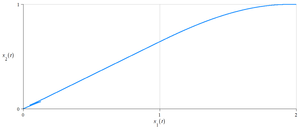
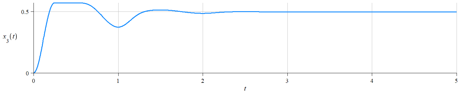
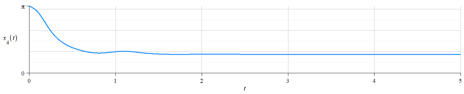
Figure 1: Projection of the trajectory of system (20), (21) on the $(x_{1},x_{2})$-plane (left) and time-plots of $x_{3}(t)$ and $x_{4}(t)$ (right).

4.2 Leader-following strategies.

To illustrate Theorem 2, consider Problem 2 for a system consisting of two unicycles, one of which (the leader) moves along the figure eight. The system dynamics is described by

$$\dot{x}^{1}=f_{1}(x^{1})u_{1}^{1}+f_{2}(x^{1})u_{2}^{1},\;\;x^{1}\in\mathbb{R}^{3},\,u^{1}=(u_{1}^{1},u_{2}^{1})^{\top}\in\mathbb{R}^{2},$$ (22)

$$\dot{x}^{L}_{1}=0.2\cos(0.1t),\,\dot{x}^{L}_{2}=-0.2,$$

$$\dot{x}^{L}_{3}=-\dfrac{0.2\sin(0.1t)\big{(}\cos^{2}(0.1t)+0.5\big{)}}{4\cos^{4}(0.1t)-3\cos^{2}(0.1t)+1},$$

where $f_{1}(x^{1})=\big{(}\cos(x_{3}^{1}),\sin(x_{3}^{1}),0\big{)}^{\top}$, $f_{2}(x^{1})=\big{(}0,0,1\big{)}^{\top}$. It is easy to see that condition (11) is satisfied with $S_{1}^{1}=\{1,2\}$, $S_{2}^{1}=\{(1,2)\}$:

$${\rm span}\big{\{}f_{1}(x^{1}),\,f_{2}(x^{1}),\,[f_{1},f_{2}](x^{1})\big{\}}=\mathbb{R}^{3}\text{ for all }x\in\mathbb{R}^{3}.$$

Then we apply Theorem 2 with

$$u_{1}^{1}=a_{1}^{1}(x^{1},x^{L})+\sqrt{\dfrac{4\pi|a_{12}^{1}(x^{1},x^{L})|}{\varepsilon}}\cos\dfrac{2\pi t}{\varepsilon},$$ (23)

$$u_{2}^{1}=a_{2}^{1}(x^{1},x^{L})+{\rm sign}(a_{12}^{1}(x^{1},x^{L}))\sqrt{\dfrac{4\pi|a_{12}(x,\gamma)|}{\varepsilon}}\sin\dfrac{2\pi t}{\varepsilon},$$

$$a_{1}^{1}(x^{1},x^{L})=(x_{1}^{1}-x_{1}^{L})\cos x_{3}+(x_{2}^{1}-x_{2}^{L})\sin x_{3}^{1},$$

$$a_{2}(x^{1},x^{L})=x_{3}^{1}-x_{3}^{L},$$

$$a_{12}(x^{1},x^{L})=(x_{1}^{1}-x_{1}^{L})\sin x_{3}^{1}-(x_{2}^{1}-x_{2}^{L})\cos x_{3}^{1}.$$

Figure 2 depicts the results of simulations for $\varepsilon=0.1$, $\gamma=10$, $d^{1}=(0.1,0.1,0)$, $x^{1}(0)=(1,0.5,0)^{\top}$, $x^{L}(0)=(0,0,\dfrac{\pi}{4})^{\top}$.

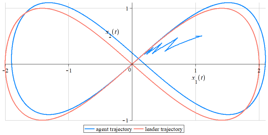
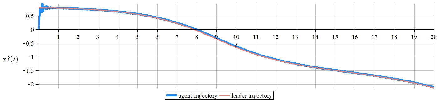
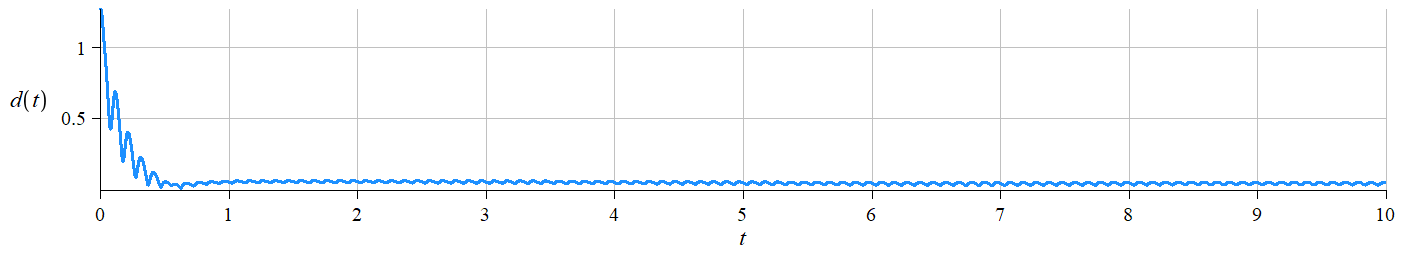
Figure 2: Projections of the trajectory of system (22) on the $(x_{1}^{1},x_{2}^{1})$- and $(x_{1}^{L},x_{2}^{L})$-planes (left) and time-plots of $x_{3}(t)$ and $d(t)=\|x^{1}-x^{L}-d^{1}\|$ (right).

5 Conclusions

As one can see from Figure 2, the proposed partially stabilizing controllers perform quite well for solving the coordination problem for nonholonomic agents. Although we have considered rather simple formulation of the leader-following problem in Section 2.3 and Section 4, we anticipate that the results of this paper will form a basis for further treatment of the general coordination problem for multi-agent systems under essentially nonlinear controllability conditions.

References

- [1] V. V. Rumyantsev and A. S. Oziraner, Stability and stabilization of motion with respect to a part of variables. Nauka, 1987 (in Russian).
- [2] A. Zuyev, “Application of control Lyapunov functions technique for partial stabilization,” in Proc. 2001 IEEE Int. Conf. on Control Applications (CCA’01), 2001, pp. 509–513.
- [3] K. Do, Z.-P. Jiang, and J. Pan, “Global partial-state feedback and output-feedback tracking controllers for underactuated ships,” Systems & Control Letters, vol. 54, no. 10, pp. 1015–1036, 2005.
- [4] J. Cochran and M. Krstic, “Nonholonomic source seeking with tuning of angular velocity,” IEEE Tran on Automatic Control, vol. 54, no. 4, pp. 717–731, 2009.
- [5] F. Mandi and N. Mišković, “Tracking underwater target using extremum seeking,” IFAC-PapersOnLine, vol. 48, no. 2, pp. 149 – 154, 2015.
- [6] Z. Hai-ping and M. Feng-xiang, “On the stability of nonholonomic mechanical systems with respect to partial variables,” Applied Mathematics and Mechanics, vol. 16, no. 3, pp. 237–245, 1995.
- [7] V. I. Vorotnikov, Partial stability and control. Springer Science & Business Media, 2012.
- [8] A. Zuyev, “Partial asymptotic stability and stabilization of nonlinear abstract differential equations,” in Proc. 42nd IEEE Conf on Decision and Control, vol. 2, 2003, pp. 1321–1326.
- [9] C. Jammazi, “On a sufficient condition for finite-time partial stability and stabilization: applications,” IMA Journal of Mathematical Control and Information, vol. 27, no. 1, pp. 29–56, 2010.
- [10] W. M. Haddad and A. L’Afflitto, “Finite-time partial stability and stabilization, and optimal feedback control,” Journal of the Franklin Institute, vol. 352, no. 6, pp. 2329–2357, 2015.
- [11] A. L. Zuyev, Partial stabilization and control of distributed parameter systems with elastic elements. Springer, 2015.
- [12] V. I. Vorotnikov, “Partial stability and control: The state-of-the-art and development prospects,” Automation and Remote Control, vol. 66, no. 4, pp. 511–561, 2005.
- [13] A. Shiriaev and O. Kolesnichenko, “On passivity based control for partial stabilization of underactuated systems,” in Proc. 39th IEEE Conf. on Decision and Control, vol. 3, 2000, pp. 2174–2179.
- [14] O. Kolesnichenko and A. S. Shiriaev, “Partial stabilization of underactuated Euler–Lagrange systems via a class of feedback transformations,” Systems & Control Letters, vol. 45, no. 2, pp. 121–132, 2002.
- [15] C. Jammazi, “Continuous and discontinuous homogeneous feedbacks finite-time partially stabilizing controllable multichained systems,” SIAM Journal on Control and Optimization, vol. 52, no. 1, pp. 520–544, 2014.
- [16] H. Chen, B. Li, B. Zhang, and L. Zhang, “Global finite-time partial stabilization for a class of nonholonomic mobile robots subject to input saturation,” International Journal of Advanced Robotic Systems, vol. 12, no. 11, p. 159, 2015.
- [17] C. Jammazi and A. Abichou, “Partial stabilizability of nonholonomic systems.” WSEAS Transactions on Systems, vol. 5, no. 5, pp. 947–952, 2006.
- [18] V. Grushkovskaya and A. Zuyev, “Partial stability concept in extremum seeking problems,” IFAC-PapersOnLine, vol. 52, pp. 682–687, 2019.
- [19] R. Olfati-Saber, J. A. Fax, and R. M. Murray, “Consensus and cooperation in networked multi-agent systems,” Proceedings of the IEEE, vol. 95, no. 1, pp. 215–233, 2007.
- [20] J. Qin, Q. Ma, Y. Shi, and L. Wang, “Recent advances in consensus of multi-agent systems: A brief survey,” IEEE Transactions on Industrial Electronics, vol. 64, no. 6, pp. 4972–4983, 2016.
- [21] D. V. Dimarogonas and K. J. Kyriakopoulos, “A feedback stabilization and collision avoidance scheme for multiple independent nonholonomic non-point agents,” in Proc. 2005 IEEE Int. Symposium on Intelligent Control, 2005, pp. 820–825.
- [22] A. Ajorlou and A. G. Aghdam, “Connectivity preservation in nonholonomic multi-agent systems: A bounded distributed control strategy,” IEEE Transactions on Automatic Control, vol. 58, no. 9, pp. 2366–2371, 2013.
- [23] Y. Cao, W. Yu, W. Ren, and G. Chen, “An overview of recent progress in the study of distributed multi-agent coordination,” IEEE Transactions on Industrial informatics, vol. 9, no. 1, pp. 427–438, 2012.
- [24] K. D. Do, “Formation tracking control of unicycle-type mobile robots with limited sensing ranges,” IEEE Transactions on Control Systems Technology, vol. 16, no. 3, pp. 527–538, 2008.
- [25] M. B. Egerstedt and X. Hu, “Formation constrained multi-agent control,” IEEE Transactions on Robotics and Automation, vol. 17, no. 6, pp. 947–951, 2001.
- [26] S. G. Loizou and K. J. Kyriakopoulos, “Navigation of multiple kinematically constrained robots,” IEEE Transactions on Robotics, vol. 24, no. 1, pp. 221–231, 2008.
- [27] C. Yoshioka and T. Namerikawa, “Formation control of nonholonomic multi-vehicle systems based on virtual structure,” IFAC Proceedings Volumes, vol. 41, no. 2, pp. 5149–5154, 2008.
- [28] S. Mastellone, D. M. Stipanovic, and M. W. Spong, “Remote formation control and collision avoidance for multi-agent nonholonomic systems,” in Proc. 2007 IEEE Int. Conf. on Robotics and Automation, 2007, pp. 1062–1067.
- [29] N. Moshtagh and A. Jadbabaie, “Distributed geodesic control laws for flocking of nonholonomic agents,” IEEE Transactions on Automatic Control, vol. 52, no. 4, pp. 681–686, 2007.
- [30] J. Zhu, J. Lu, and X. Yu, “Flocking of multi-agent non-holonomic systems with proximity graphs,” IEEE Trans. on Circuits and Systems I: Regular Papers, vol. 60, no. 1, pp. 199–210, 2012.
- [31] W. Dong and J. A. Farrell, “Cooperative control of multiple nonholonomic mobile agents,” IEEE Transactions on Automatic Control, vol. 53, no. 6, pp. 1434–1448, 2008.
- [32] L. Cheng, Z.-G. Hou, and M. Tan, “Decentralized adaptive consensus control for multi-manipulator system with uncertain dynamics,” in 2008 IEEE Int. Conf. on Systems, Man and Cybernetics, 2008, pp. 2712–2717.
- [33] Y.-C. Liu and N. Chopra, “Controlled synchronization of heterogeneous robotic manipulators in the task space,” IEEE transactions on Robotics, vol. 28, no. 1, pp. 268–275, 2011.
- [34] H. G. Tanner, S. G. Loizou, and K. J. Kyriakopoulos, “Nonholonomic navigation and control of cooperating mobile manipulators,” IEEE Transactions on Robotics and Automation, vol. 19, no. 1, pp. 53–64, 2003.
- [35] A. Zuyev, “Exponential stabilization of nonholonomic systems by means of oscillating controls,” SIAM Journal on Control and Optimization, vol. 54, no. 3, pp. 1678–1696, 2016.
- [36] A. Zuyev, V. Grushkovskaya, and P. Benner, “Time-varying stabilization of a class of driftless systems satisfying second-order controllability conditions,” in Proc. 15th European Control Conference, 2016, pp. 1678–1696.
- [37] V. Grushkovskaya and A. Zuyev, “Obstacle avoidance problem for second degree nonholonomic systems,” in Proc. 57th IEEE Conf. on Decision and Control, 2018, pp. 1500–1505.
- [38] Z. Li and J. Canny, “Motion of two rigid bodies with rolling constraint,” IEEE Transactions on Robotics and Automation, vol. 6, no. 1, pp. 62–72, 1990.