Quantum three body problems using harmonic oscillator bases with different sizes

Abstract

We propose a new treatment for the quantum three-body problem. It is based on an expansion of the wave function on harmonic oscillator functions with different sizes in the Jacobi coordinates. The matrix elements of the Hamiltonian can be calculated without any approximation and the precision is restricted only by the dimension of the basis. This method can be applied whatever the system under consideration. In some cases, the convergence property is greatly improved in this new scheme as compared to the old traditional method. Some numerical tricks to reduce computer time are also presented.

I Introduction

The quantum problem of three interacting particles is a very old one, since it is present in very different domains of physics: molecular, atomic, nuclear and hadronic physics among others. Besides the fact that there exists a large number of such systems in nature, it is interesting because it is much more difficult to solve than the relatively easy two-body problem. One difficulty comes from the fact that statistical approaches or even many-body technics are not efficient for three-body problems; in particular a good treatment of the center of mass is necessary and internal coordinates must be employed. Another difficulty appears if the three particles are identical; in that case one must fulfill the Pauli principle which is not easy to manage with internal coordinates.

There exists a lot of different technics to solve the three-body problem; let us cite, among others, quantum Monte Carlo method carl ; lind ; ham , Faddeev equations gloc , hyperspherical formalism flr , stochastic variational method suz , expansion on orthogonal bases, for example harmonic oscillator (OH) isg ; sil96 . In principle, all these methods tend to the exact result if some parameters (number of states, number of amplitudes, number of mesh points,…) tend to infinity. The convergence properties depend not only on the type of method, but also on the system and the dynamics themselves. Of course, one searches the minimum of computational effort for a given precision. Each method has its own advantages and its own drawbacks. For example, dealing with a semirelativistic kinematics is not an easy task with Faddeev or hyperspherical formalism on a mesh, hard core or very short range repulsive potentials are very difficult to implement with the stochastic variational method or the HO basis.

The aim of this paper is to revisit the HO method to accelerate the convergence of the results. So we want to obtain the same precision with an expansion needing less quanta, and thus less basis states. Besides the fact that a smaller number of quanta means less storing memory and less computational time, it has also the advantage to give a more physical idea of the wave function. Indeed if we obtain a good wave function with, let say, $N=1000$ basis states the physical interpretation of this wave function is difficult; on the other hand if we get the same precision with $N=10$ basis states, one grasps better the physical contents of the system because the degrees of freedom chosen are more adapted to it. Moreover, if we are interested by some observable built from this wave function the gain is even more impressive. To obtain the average value of the operator on the calculated wave function, the first case needs to compute one million terms, whereas one hundred terms are enough in the second case.

The traditional approach based on HO basis considers that the harmonic oscillator wave function have the same size (or the same scale) in both Jacobi coordinates. This was an unavoidable requirement to calculate rapidly and precisely the matrix elements of the potential within this basis. If the three particles have the same mass, as in most problems of nuclear physics, this condition is not a flaw; but if the particles have very different masses this condition is not well suited because the basis states can hardly reproduce the physical asymmetry. This paper presents a method to deal with this asymmetry by using HO wave functions with different sizes for different Jacobi coordinates. One can be very skeptical on the possibility to calculate rigorously the matrix elements in such a basis because it is known that expanding a HO wave function with one size on a basis of HO wave functions with another size requires an infinite number of terms. However, we will show that we perfectly achieve this goal if we define correct changes of variables. This possibility opens the door to a better convergence of the method.

We are aware that the present method cannot compete with more sophisticated technics to obtain a very precise result close to the exact one; but the price to pay is also much less. So, we believe that it is a good compromise between computational and technical difficulties and precision of the results. A serious advantage of this approach is that the use of a relativistic kinematics is not a problem; the Fourier transform of a HO function is again a HO function so that the matrix elements of the operator are easily calculated in momentum representation. Another interesting advantage of using a HO basis is its universality; it is systematic so that dealing with orbitally or radially excited states is of the same difficulty than dealing with the ground state. This is not the case for most of other methods.

The paper is organized as follows. In the next section, we develop the theory with special accent put on the differences with the traditional formalism. In Sec. III we present some numerical aspects that allowed us to gain comfortable computer time. In Sec. IV a detailed analysis of convergence properties, as well as a simple application are discussed. In the last section the conclusions are drawn. Some very technical details are relegated in the appendices.

II Theory

II.1 Jacobi coordinates

Each particle $i$ ($i$=1, 2, 3) is characterized by a mass $m_{i}$ and by various dynamical degrees of freedom: internal degrees of freedom symbolized generically by $\alpha_{i}$ and by its position ${\bf r}_{i}$ in a given reference frame. In case of electrons for atomic physics $\alpha_{i}$ stands for spin and the corresponding magnetic number; in the case of nucleons for nuclear physics $\alpha_{i}$ includes, in addition to spin, isospin degrees of freedom, while in the case of quarks for subnuclear physics $\alpha_{i}$ includes, in addition to spin and isospin, color degrees of freedom. The conjugate momentum of ${\bf r}_{i}$ is denoted ${\bf p}_{i}$. Let us define by $m$ an arbitrary reference mass and the dimensionless parameters $\omega_{i}=m_{i}/m$, $\omega_{ij}=\omega_{i}+\omega_{j}$, $\omega=\omega_{1}+\omega_{2}+\omega_{3}$.

In order to treat correctly the center of mass motion, it is necessary to introduce the center of mass position ${\bf R}$ and the total momentum ${\bf P}$, defined as usual

$${\bf R}=\frac{\omega_{1}{\bf r_{1}}+\omega_{2}{\bf r_{2}}+\omega_{3}{\bf r_{3}}}{\omega}\quad;\quad{\bf P}={\bf p}_{1}+{\bf p}_{2}+{\bf p}_{3}.$$ (1)

The dimensionless Jacobi coordinates ${\bf x}$ and ${\bf y}$ corresponding to internal relative positions can be defined with several prescriptions.

For people working with traditional HO functions, the usual definition is

$$b\,{\bf x}=\sqrt{\frac{2\omega_{2}\omega_{3}}{\omega_{23}}}\>({\bf r}_{2}-{\bf r}_{3})\quad;\quad b\,{\bf y}=\sqrt{\frac{2\omega_{1}\omega_{23}}{\omega}}\>\left(\frac{\omega_{2}{\bf r}_{2}+\omega_{3}{\bf r}_{3}}{\omega_{23}}-{\bf r}_{1}\right).$$ (2)

Here, the scale parameter $b$ implies a unique size for HO functions. The deep reason for choosing such a precise definition is the following; when dealing with the potential, one needs to express the Jacobi coordinates that are derived from a permutation of the particles. With the choice (2) all these Jacobi coordinates are related by orthogonal transformations; this nice property allows to simplify a lot the numerical calculations. The parameter $b$ can be determined from a variational procedure.

In our approach we introduce two scale parameters, one for each Jacobi coordinate, so that we define more simply

$$b_{x}\,{\bf x}=({\bf r}_{2}-{\bf r}_{3})\quad;\quad b_{y}\,{\bf y}=\frac{\omega_{2}{\bf r}_{2}+\omega_{3}{\bf r}_{3}}{\omega_{23}}-{\bf r}_{1}.$$ (3)

The two parameters $b_{x}$ and $b_{y}$ can also be determined by a variational procedure. For arbitrary values of $b_{x}$ and $b_{y}$, both definitions (2) and (3) of the Jacobi coordinates obviously differ; they are nevertheless identical if we impose the relationship

$$b_{x}=b\sqrt{\frac{\omega_{23}}{2\omega_{2}\omega_{3}}}\quad{\rm and}\quad b_{y}=b\sqrt{\frac{\omega}{2\omega_{1}\omega_{23}}}.$$ (4)

Thus, our new theory must coincide with the old one if we maintain the conditions (4). This is a drastic check for our numerical codes.

The conjugate momenta corresponding to ${\bf x}$ and ${\bf y}$ are denoted ${\bf p}$ and ${\bf q}$ respectively. Their expression in terms of ${\bf p}_{i}$ are straightforward.

II.2 Basis states

With those definitions (3), particle 1 plays a special role and the natural coupling is [1(23)]. Nevertheless we have the freedom to choose the particle order. If we were able to perform a rigorous treatment (number of quanta infinite), this order would be irrelevant; however the expansion is truncated, the order makes a difference, and there exists a special order which gives better results. We will show an example later.

The total wave function $\Psi$ is expanded on basis states

$$\Psi({\bf x},{\bf y})=\sum_{i=1}^{N}\eta_{\sigma_{i}}\Phi_{k_{i}}({\bf x},{\bf y}).$$ (5)

In this expression $\eta_{\sigma_{i}}$ is the part of the wave function corresponding to the internal degrees of freedom (spin, isospin, color) and means symbolically $[\alpha_{1}(\alpha_{2}\alpha_{3})_{\sigma}]_{\alpha}$; the various indices $\sigma$ stand for the intermediate couplings and correspond to a finite number of states. The space part $\Phi_{k_{i}}({\bf x},{\bf y})$ is a coupled product of two HO functions

$$\Phi_{k}({\bf x},{\bf y})=[\phi_{nl}({\bf x})\phi_{\nu\lambda}({\bf y})]_{L},$$ (6)

where $n$ ($\nu$) and $l$ ($\lambda$) are the radial and orbital quantum numbers for the Jacobi coordinate ${\bf x}$ (${\bf y}$); $L$ is the orbital angular momentum of the system, and the index $k$ gathers the quantum numbers ${n,l,\nu,\lambda,L}$. The functions $\phi_{nlm}({\bf x})$ = $\frac{u_{nl}(x)}{x}Y_{lm}(\hat{x})$ are the usual HO wave functions, defined in any textbook on quantum mechanics. In the following, we will use extensively the matrix elements

$$V_{nl,n^{\prime}l^{\prime}}(a)=\langle\phi_{nl}({\bf x})\mid V(ax)\mid\phi_{n^{\prime}l^{\prime}}({\bf x})\rangle=\delta_{ll^{\prime}}\int_{0}^{\infty}u_{nl}(x)u_{n^{\prime}l}(x)V(ax)dx.$$ (7)

An efficient method to calculate them is discussed later on.

An interesting property of the space functions (6) is the orthogonality condition

$$\langle\Phi_{k}({\bf x},{\bf y})\mid\Phi_{k^{\prime}}({\bf x},{\bf y})\rangle=\delta_{kk^{\prime}},$$ (8)

which is valid whatever the size parameters.

The number of quanta of the function (6) is simply $2n+l+2\nu+\lambda$. In the expansion of the total wave function (5), we always consider all the basis states (6) with a number of quanta less or equal to a given number $N_{Q}$. This prescription is absolutely fundamental to treat correctly the Pauli principle (see Sec. II.5).

II.3 The Hamiltonian

Since our approach is essentially of type “potential model” the Hamiltonian takes the traditional form

$$H=T+V.$$ (9)

We are able to treat equally well both types of kinetic energy operator $T$, nonrelativistic or semirelativistic.

The nonrelativistic operator is given by

$$T=T_{\rm nr}=\sum_{i=1}^{3}\frac{{\bf p}_{i}^{2}}{2m_{i}}-\frac{{\bf P}^{2}}{2M}=\frac{{\bf p}^{2}}{2\mu_{p}}+\frac{{\bf q}^{2}}{2\mu_{q}},$$ (10)

where $M=\omega m$ is the total mass and where $\mu_{p}$ and $\mu_{q}$ are quantities proportional to the reduced masses. They are defined by

$$\mu_{p}=\frac{mb_{x}^{2}\omega_{2}\omega_{3}}{\omega_{23}}\quad;\quad\mu_{q}=\frac{mb_{y}^{2}\omega_{1}\omega_{23}}{\omega}.$$ (11)

The semirelativistic operator needs to be evaluated in the rest frame $\bf P=0$; hence, we have

$$T=T_{\rm sr}=\sum_{i=1}^{3}\sqrt{{\bf p}_{i}^{2}+m_{i}^{2}}-M=K_{1}+K_{2}+K_{3}-M.$$ (12)

In the rest frame the expression of each term is written

$$K_{1} = \sqrt{\frac{{\bf q}^{2}}{b_{y}^{2}}+\omega_{1}^{2}m^{2}},$$

$$K_{2} = \sqrt{\left(\frac{\omega_{2}{\bf q}}{b_{y}\,\omega_{23}}+\frac{{\bf p}}{b_{x}}\right)^{2}+\omega_{2}^{2}m^{2}},$$

$$K_{3} = \sqrt{\left(\frac{\omega_{3}{\bf q}}{b_{y}\,\omega_{23}}-\frac{{\bf p}}{b_{x}}\right)^{2}+\omega_{3}^{2}m^{2}}.$$ (13)

Although it is possible to deal with three-body forces in this formalism, we consider in this paper only two-body forces

$$V=V_{12}+V_{13}+V_{23},$$ (14)

where $V_{ij}$ represents the interaction between particle $i$ and particle $j$. It can be decomposed generally as

$$V_{ij}=\sum_{s}\hat{O}_{ij}^{(s)}V_{ij}^{(s)}(\mid{\bf r}_{i}-{\bf r}_{j}\mid),$$ (15)

where $\hat{O}_{ij}^{(s)}$ is the operator acting in the space of internal degrees of freedom (spin, isospin, color). There exist in general several different structures $(s)$ compatible with invariance symmetries. The most general potential must take care of all these possibilities by a summation over the various structures. The space part for a given structure is the form factor $V_{ij}^{(s)}(\mid{\bf r}_{i}-{\bf r}_{j}\mid)$.

II.4 Matrix elements

II.4.1 Brody-Moshinsky coefficients

The calculation of the matrix elements in the basis (6) is one of the novelties developed in this paper. It is based on the use of generalized Brody-Moshinsky (or Smirnov) coefficients (BMC). This technique was employed long time ago by nuclear physicists but seems to be not often used nowadays. One can find the interesting properties of BMC in several textbooks (see for example law ; bro ) or papers sil85 . The only thing that is needed here is that they relate HO functions with arguments that are transformed by a rotation. More explicitly, we have

$$[\phi_{n_{1}l_{1}}({\bf r}\cos\beta+{\bf R}\sin\beta)\phi_{n_{2}l_{2}}(-{\bf r}\sin\beta+{\bf R}\cos\beta)]_{\lambda} =$$

$$\sum_{n,l,N,L}\langle nlNL;\lambda\mid n_{1}l_{1}n_{2}l_{2};\lambda\rangle_{\beta}[\phi_{nl}({\bf r})\phi_{NL}({\bf R})]_{\lambda}.$$ (16)

The various quantum numbers appearing in the BMC $\langle nlNL;\lambda\mid n_{1}l_{1}n_{2}l_{2};\lambda\rangle_{\beta}$ are constrained by triangular inequalities, by parity conservation and by conservation of the number of quanta.

II.4.2 kinetic energy

The matrix elements for the non-relativistic operator (10) are very well known

$$\langle\Phi_{k_{i}}\mid T_{\rm nr}\mid\Phi_{k_{j}}\rangle=\delta({\bar{k}}_{i},{\bar{k}}_{j})K_{p}(n_{i},n_{j})+\delta({\bar{k}}_{i},{\bar{k}}_{j})K_{q}(\nu_{i},\nu_{j}),$$ (17)

where the notation $\delta({\bar{k}}_{i},{\bar{k}}_{j})$ means the Kronecker symbol for every quantum number of the basis except those appearing in the matrix element in front of it ($K_{p}$ for the first, $K_{q}$ for the second). This last term is given by

$$K_{p}(n_{i},n_{j}) = \frac{1}{2\mu_{p}}\left[(2n_{i}+l_{i}+3/2)\delta_{n_{i},n_{j}}+\sqrt{n_{i}(n_{i}+l_{i}+1/2)}\delta_{n_{i},n_{j}+1}\right.$$ (18)

$$+ \left.\sqrt{n_{j}(n_{j}+l_{j}+1/2)}\delta_{n_{j},n_{i}+1}\right],$$

and an analogous expression for $K_{q}$.

The matrix elements for the semirelativistic operators (II.3) seem more complicated. However, it is convenient to work in momentum representation. Indeed the Fourier transform of the space function (6) is exactly of the same form (with an extra phase factor) with ${\bf p}$ and ${\bf q}$ replacing ${\bf x}$ and ${\bf y}$. The first term $K_{1}$ of the operator is thus very easy to calculate

$$\langle\Phi_{k_{i}}\mid K_{1}\mid\Phi_{k_{j}}\rangle=\delta({\bar{k}}_{i},{\bar{k}}_{j})\frac{(-1)^{\nu_{i}+\nu_{j}}}{b_{y}}{\cal K}_{\nu_{i}\lambda_{i},\nu_{j}\lambda_{j}}(b_{y}m\omega_{1}),$$ (19)

where the dynamical ingredient $\cal K$ is reduced to a single integral

$${\cal K}_{nl,NL}(\mu)=\int_{0}^{\infty}dq\,u_{nl}(q)u_{NL}(q)\sqrt{q^{2}+\mu^{2}}.$$ (20)

The idea for calculating the matrix elements of $K_{2}$ relies on a trick that can be applied with adaptation to the other matrix elements. We remark that, in $K_{2}$, the vector present under the square root, namely $\frac{\omega_{2}{\bf q}}{b_{y}\omega_{23}}+\frac{\bf p}{b_{x}}$, can be made proportional to some vector ${\bf r}$ which is obtained from ${\bf p}$ and ${\bf q}$ by a rotation with some angle $\beta_{1}$. One introduces the vector ${\bf s}$ orthogonal to ${\bf r}$ and moves, with help of BMC, from (${\bf p}$,${\bf q}$) representation for HO to the (${\bf r}$,${\bf s}$) representation. The calculation of the matrix element in this representation is then quite easy. The final result is

$$\langle\Phi_{k_{i}}\mid K_{2}\mid\Phi_{k_{j}}\rangle = \delta({\bar{k}}_{i},{\bar{k}}_{j})\frac{\pi_{2}}{\eta_{1}}\sum_{n_{2},l_{2},\nu_{2},\nu_{2}^{\prime},\lambda_{2}}(-)^{\nu_{2}+\nu_{2}^{\prime}}\langle\nu_{2}\lambda_{2}n_{2}l_{2};L_{i}\mid n_{j}l_{j}\nu_{j}\lambda_{j};L_{i}\rangle_{\beta_{1}}$$ (21)

$$\langle\nu_{2}^{\prime}\lambda_{2}n_{2}l_{2};L_{i}\mid n_{i}l_{i}\nu_{i}\lambda_{i};L_{i}\rangle_{\beta_{1}}{\cal K}_{\nu_{2}^{\prime}\lambda_{2},\nu_{2}\lambda_{2}}(\eta_{1}m\omega_{2}).$$

The phase is $\pi_{2}=(-1)^{l_{i}+l_{j}}$ and we have introduced geometrical factors

$$\alpha_{1} = \frac{\sqrt{b_{x}^{2}\omega_{2}^{2}+b_{y}^{2}\omega_{23}^{2}}}{\omega_{23}},$$

$$\eta_{1} = \frac{b_{x}b_{y}}{\alpha_{1}},$$ (22)

and the angle for the rotation

$$\cos\beta_{1}=\frac{b_{y}}{\alpha_{1}}\quad;\quad\sin\beta_{1}=\frac{b_{x}\,\omega_{2}}{\alpha_{1}\,\omega_{23}}.$$ (23)

The matrix element for the $K_{3}$ term is obtained exactly with the same trick. The result can be obtained from (21) with the phase $\pi_{3}=1$, with other geometrical factors $\alpha_{2}$, $\eta_{2}$, and a rotation angle $\beta_{2}$ deduced from $\alpha_{1}$, $\eta_{1}$, $\beta_{1}$ by replacing $\omega_{2}$ by $\omega_{3}$.

II.4.3 Potential energy

In calculating the matrix elements of the potential operator, one can focus on the operator (15) acting on the pair $kl$. Then

$$\langle\eta_{\sigma_{i}}\Phi_{k_{i}}\mid V_{kl}\mid\eta_{\sigma_{j}}\Phi_{k_{j}}\rangle=\sum_{s}{\cal O}_{ij}^{(s)}(kl){\cal E}_{ij}^{(s)}(kl),$$ (24)

where ${\cal O}_{ij}^{(s)}(kl)$ is the matrix element of the internal operator between the internal wave functions. It is calculated in practice by Racah techniques. We are interested here by the matrix element concerned with the space part

$${\cal E}_{ij}^{(s)}(kl)=\langle\Phi_{k_{i}}\mid V_{kl}^{(s)}(\mid{\bf r}_{k}-{\bf r}_{l}\mid)\mid\Phi_{k_{j}}\rangle.$$ (25)

The term $V_{23}$ is easy to calculate since the argument entering this term is precisely one of the Jacobi coordinate. One gets

$${\cal E}_{ij}^{(s)}(23)=\delta({\bar{k}}_{i},{\bar{k}}_{j})V_{n_{i}l_{i},n_{j}l_{j}}^{(s)}(b_{x})$$ (26)

with the definition (7) for the matrix element in the HO basis.

The calculation for $V_{13}$ is more involved but can be performed with the same trick as the one used for $K_{2}$. The argument ${\bf r}_{13}$ appearing in the potential can be put in the form ${\bf r}_{13}=\alpha_{1}{\bf u}$ with the vector ${\bf u}$ obtained from ${\bf x}$ and ${\bf y}$ by a rotation with the angle $\beta_{1}$. The coefficients $\alpha_{1}$ and $\beta_{1}$ are already defined in (II.4.2) and (23). One then introduces the vector ${\bf v}$ orthogonal to vector ${\bf u}$. The basis state are HO functions with (x,y) representation; with appropriate BMC we change them into HO functions with (u,v) representation. In this representation, the matrix element is obvious. The result is

$${\cal E}_{ij}^{(s)}(13) = \delta_{L_{i}L_{j}}\pi_{2}\sum_{n_{2},n_{2}^{\prime},l_{2},\nu_{2},\lambda_{2}}\langle\nu_{2}\lambda_{2}n_{2}l_{2};L_{i}\mid n_{j}l_{j}\nu_{j}\lambda_{j};L_{i}\rangle_{\beta_{1}}$$ (27)

$$\langle\nu_{2}\lambda_{2}n_{2}^{\prime}l_{2};L_{i}\mid n_{i}l_{i}\nu_{i}\lambda_{i};L_{i}\rangle_{\beta_{1}}V_{n_{2}^{\prime}l_{2},n_{2}l_{2}}^{(s)}(\alpha_{1}).$$

The calculation for $V_{12}$ is performed in an analogous way; the value of ${\cal E}_{ij}^{(s)}(12)$ has the same expression as (27) but with a phase $\pi_{3}=1$ and with $\alpha_{2}$ and $\beta_{2}$ replacing $\alpha_{1}$ and $\beta_{1}$.

II.4.4 Differences with the usual method

In this part, we want to point out what are the complications due to the use of HO functions with different sizes as compared to the traditional method based on HO functions with a unique size.

First, the number of basic states is a geometrical property based on invariance principles acting on quantum numbers; thus, for a given number of quanta $N_{Q}$, the number of basis states in both methods is exactly the same. The diagonalization procedure takes more or less the same time.

Now, one must examine the time needed to compute the matrix elements. In fact, one should realize that their formal expressions are exactly the same in both approaches. Thus, if we suppose that $b,b_{x},b_{y}$ are given once for all, the new method is as easy (or as difficult!) and as fast as the old one.

The difference is merely in the determination of the size parameters. In both method they are determined by requiring a minimum for the energy of a particular state. In the old method we have only one parameter $b$ whereas in this new method the minimization must be done in a two dimensional space ($b_{x},b_{y}$). This results of course in a larger time. But there is also another complication which is less transparent. In the old method the BMC to be used in the formalism depend only on the $\omega_{i}$ parameters (on the system) but not on the $b$ parameter; this was the reason for choosing the special set of Jacobi coordinates (2). Thus they can be calculated once for all at the beginning of the code and remain the same during the variational procedure. In the new method the BMC depend both on $\omega_{i}$ and ($b_{x},b_{y}$) (see relations (21) and (23)) so that they need to be recalculated at each step of the variational procedure. At first sight this may seem a dramatic drawback; however this must be moderated because BMC are computed very fast, and also because, for the same precision, the matrices in the new method are smaller than in the old one. All these aspects are commented later on.

II.5 Identical particles

In the case of two identical particles, it is natural to consider them as the objects 2 and 3, with the set of Jacobi coordinates chosen (3). It is then easy to select, in all the possible basis states, those characterized by the good symmetry property. This implies some constraints (depending on the fact that the particles are fermions or bosons) on the quantum numbers of the wave functions associated with the variable x. The basis is then smaller (roughly by a factor 2) than in the case of three different particles, and it can be also shown that

$$\langle\Phi_{k_{i}}\mid K_{2}\mid\Phi_{k_{j}}\rangle = \langle\Phi_{k_{i}}\mid K_{3}\mid\Phi_{k_{j}}\rangle,$$

$$\langle\eta_{\sigma_{i}}\Phi_{k_{i}}\mid V_{12}\mid\eta_{\sigma_{j}}\Phi_{k_{j}}\rangle = \langle\eta_{\sigma_{i}}\Phi_{k_{i}}\mid V_{13}\mid\eta_{\sigma_{j}}\Phi_{k_{j}}\rangle.$$ (28)

Consequently, the computation labor is in this case greatly reduced.

When the three particles are identical, it is not obvious to build the basis states in such a way that they are all completely symmetrical or antisymmetrical for the permutation of the particles. If we diagonalize the Hamiltonian in the basis for which particles 2 and 3 have already good symmetry properties, we obtain eigenstates which are either completely symmetrical, completely antisymmetrical, or of mixed symmetry. A way to distinguish all these states is to calculate for each state the mean value of the transposition operator $P_{13}$ for particles 1 and 3. The completely symmetrical (antisymmetrical) states will be characterized by $\langle P_{13}\rangle=+1$ ($-1$). One can thus imagine to let the Hamiltonian do the job to filter states with given symmetry, verify a posteriori the symmetry of eigenstates, and reject those having a symmetry not compatible with the Pauli principle. Practically this procedure cannot be applied systematically because very often there exist degenerate states with different symmetries.

This is why we adopt an approach which is more painful but which works correctly each time. In practice, we diagonalize the operator $P_{13}$ in the basis symmetrized for particles 2 and 3. We select the eigenstates with eigenvalues $+1$ or $-1$ according to the nature of our particles. Then we diagonalize the Hamiltonian in the basis built with the selected eigenstates. We can also perform the inverse basis change to obtain the Hamiltonian eigenstates expressed in the original basis.

We have to compute the matrix elements $\langle\eta_{\sigma_{i}}\Phi_{k_{i}}\mid P_{13}\mid\eta_{\sigma_{j}}\Phi_{k_{j}}\rangle$. The mean value of the operator for color, isospin and spin degrees of freedom is very easy to calculate by usual Racah techniques. The computation for the space part is much more involved. Let us note (${\bf x}^{\prime},{\bf y}^{\prime}$) the coordinates resulting of the action of $P_{13}$ on the coordinates (${\bf x},{\bf y}$). Then we have

$$\langle\Phi_{k_{i}}({\bf x},{\bf y})\mid P_{13}\mid\Phi_{k_{j}}({\bf x},{\bf y})\rangle=\langle\Phi_{k_{i}}({\bf x},{\bf y})\mid\Phi_{k_{j}}({\bf x}^{\prime},{\bf y}^{\prime})\rangle.$$ (29)

The trick is to introduce new sets of coordinates (${\bf u},{\bf v}$) and rotations $\cal R$ of angle $\varphi$ such that, for instance,

$$\left(\begin{array}[]{c}{\bf x}^{\prime}\\ {\bf y}^{\prime}\end{array}\right)={\cal R}\left(\begin{array}[]{c}{\bf u}\\ {\bf v}\end{array}\right)\quad{\rm and}\quad\left(\begin{array}[]{c}{\bf x}\\ {\bf y}\end{array}\right)={\cal R}\left(\begin{array}[]{c}{\bf v}/\sqrt{\alpha}\\ \sqrt{\alpha}\,{\bf u}\end{array}\right).$$ (30)

It is then possible to calculate the matrix element (29)

$$\langle\Phi_{k_{i}}\mid P_{13}\mid\Phi_{k_{j}}\rangle = \delta_{L_{i}L_{j}}\ \ \pi(r)\sum_{n_{1},n_{1}^{\prime},l_{1},\nu_{1},\nu_{1}^{\prime},\lambda_{1}}\langle\nu_{1}^{\prime}\lambda_{1}n_{1}^{\prime}l_{1};L_{i}\mid n_{j}l_{j}\nu_{j}\lambda_{j};L_{i}\rangle_{\varphi}$$ (31)

$$\langle n_{1}l_{1}\nu_{1}\lambda_{1};L_{i}\mid n_{i}l_{i}\nu_{i}\lambda_{i};L_{i}\rangle_{\varphi}\>F_{n_{1}^{\prime}n_{1}l_{1}}(\sqrt{\alpha})\>F_{\nu_{1}^{\prime}\nu_{1}\lambda_{1}}(1/\sqrt{\alpha}),$$

where

$$\alpha=\frac{16r^{4}+8r^{2}+9+\rho}{32r^{2}},\quad\rho=\sqrt{(4r^{2}-3)^{2}(16r^{4}+40r^{2}+9)},\quad r=\frac{b_{y}}{b_{x}},$$

$$\cos\varphi=\sqrt{\frac{\rho-16r^{4}+9}{2\rho}},\quad\sin\varphi=\sqrt{\frac{\rho+16r^{4}-9}{2\rho}},\quad{\rm and}$$

$$\pi(r)=(-1)^{\lambda_{i}+l_{i}+L_{i}}\quad{\rm if}\quad r<\sqrt{3}/2\quad{\rm or}\quad\pi(r)=(-1)^{\lambda_{i}+l_{j}+L_{i}}\quad{\rm if}\quad r>\sqrt{3}/2.$$ (32)

The quantity $F_{n^{\prime}nl}(a)$ measures the overlap of one HO function with another one scaled by a positive factor

$$F_{n^{\prime}nl}(a)=a^{3/2}\int_{0}^{\infty}u_{n^{\prime}l}(x)\>u_{nl}(ax)\>dx.$$ (33)

Its analytical expression as well as its symmetry properties are given in Ref. sema95 .

From Eq. (31), it appears that the operator $P_{13}$ couples basis states which can be characterized by different numbers of quanta. Consequently, in a basis truncated at a fixed number of quanta, it is not possible to obtain an integer value for $\langle P_{13}\rangle$, that is to say an eigenstate with a well defined symmetry. Such an eigenstate needs an infinite number of basis states to develop.

Nevertheless, if $b_{y}/b_{x}=\sqrt{3}/2$, that is to say if the relationship (4) is verified, we have $\alpha=1$ and $\varphi=\pi/6$, which implies

$$\langle\Phi_{k_{i}}\mid P_{13}\mid\Phi_{k_{j}}\rangle=\delta_{L_{i}L_{j}}(-1)^{\lambda_{i}+l_{i}+L_{i}}\langle\nu_{j}\lambda_{j}n_{j}l_{j};L_{i}\mid n_{i}l_{i}\nu_{i}\lambda_{i};L_{i}\rangle_{\pi/6}.$$ (34)

In this case, two basis states with different numbers of quanta are not mixed by the operator $P_{13}$, and it is possible to obtain an eigenstate with a defined symmetry in a basis truncated at a fixed number of quanta. This is the reason why we work in such bases, as mentioned above.

To study systems with three identical particles we must choose between two procedures. We can work with $b_{x}$ and $b_{y}$ completely free to compute the lowest possible upper bounds, but the price to pay is to obtain eigenstates which are not characterized by a defined symmetry. On contrary, we can impose the constraint (4) on $b_{x}$ and $b_{y}$ to get eigenstates with a defined symmetry, but with the risk to not obtain the lowest possible upper bounds. In all cases studied, we remarked that it is preferable to work with the second procedure because the loss of good symmetry properties results in an increase of the upper bounds which cannot be compensated by relaxing the constraint (4). Actually, the asymmetry between Jacobi coordinates is less pronounced in three identical particle systems, it is then not a serious penalty to work with only one effective variational parameter for such systems.

III Numerical aspects

This section is devoted to some tricks that we employed in our numerical codes to fasten the computations.

As we saw just before, the BMC need to be calculated very often, each time as we change one of the size parameters. Moreover, if the number of quanta increases, the number of BMC required increases also drastically. The algorithm to calculate them has been explained in detail in Ref. sil85 ; it relies on recursive formulae which are precise and fast enough. In order to be efficient this algorithm needs to calculate all of them up to a given number of quanta $N_{Q}$ even if they are not all necessary for our calculations. Table 1 shows the total number of BMC as a function of $N_{Q}$. In our calculations we have pushed the expansion up to $N_{Q}=16$. The great advantage of this algorithm is that the BMC are stored naturally in such a way that the elements needed in the various summations where they appear (summations over $n,l,\nu,\lambda$) are placed contiguously in a one dimensional array so that the summation is restricted to a reading in sequence which is very fast.

Another time consuming part of our job, is the calculation of the matrix elements (7) which appear in the inner loops of our codes. There exists a very old way, that is also often forgotten, to calculate them precisely and very fast. The technique relies on Talmi’s integrals and was reported elsewhere sema95 . More details are provided in the appendix A. Let us just mention that most of Talmi’s integral of practical use can be evaluated analytically; this is important because they depend on the size parameters and must be calculated very often.

IV Results

Our method can be applied to a wide variety of three particle systems. In this paper we study the convergence rate with baryons considered as three quark systems. We report some results obtained with a nonrelativistic potential model which can describe quite well meson and baryon spectra bhad81 , and two simple potential models developed to compare nonrelativistic and semirelativistic approaches fulc94 .

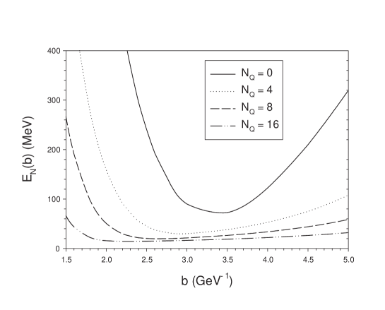
Figure 1: Binding energy of the nucleon $E_{N}$ for the potential of Bhaduri et al. bhad81 as a function of the number of quanta $N_{Q}$ and the unique oscillator length $b$.

The quality of an upper bound depends on two kinds of parameters: the number of quanta and the oscillator length parameters. In the case of three identical particles, we have mentioned that it is preferable to work with an unique parameter $b$ (see Sec. II.5). In Fig. 1, the nucleon mass $M_{N}$ for the model of Ref. bhad81 is plotted as a function of $b$ for different values of the number of quanta $N_{Q}$. For small values of $N_{Q}$, a good choice of $b$ is crucial, but as $N_{Q}$ increases, the minimum of the curve $M_{N}(b)$ becomes more and more flat. In order to save computation time, it is interesting to compute a given upper bound in two steps. First, determine the optimum value of the oscillator parameter for this upper bound computed with a small value of the number of quanta, say $N^{\prime}_{Q}$. Secondly, use this value of the oscillator parameter to recompute the upper bound with a higher value of the number of quanta, say $N_{Q}$. This situation is illustrated in Table 2 for two $I=S=1/2$ lowest state baryons within the model of Ref. bhad81 . We can see that for baryon containing at least two different particles, it is also interesting to use this procedure. In the following we will always take $N^{\prime}_{Q}=8$. The maximum number of quanta used in this paper is $N_{Q}=16$. A higher value is not considered for practical reasons (see Table 1 and appendix  A). The method used to determine the optimum values of length parameters is described in appendix B.

We will now see that good upper bounds can be obtained with the procedure described above. First look at the case of 3 identical particles, for which it is preferable to use the constraint (4) on length parameters. In Table 3, binding energies of the center of gravity $N-\Delta$ for the nonrelativistic and semirelativistic Fulcher’s models fulc94 are given as a function of the number of quanta $N_{Q}$. For both kinematics, the convergence is reached at $N_{Q}=16$.

In the cases of asymmetric systems, we can expect that the use two nonlinear parameters will bring some advantages. In Table 4, binding energies of the lowest state $ubb$ baryon, for the nonrelativistic Fulcher’s models fulc94 , are given as a function of the number of quanta $N_{Q}$, for two values of $L$. For the $L=0$ state, the use of two oscillator lengths yields only a very small improvement for a small number of quanta. This improvement even vanishes when the number of quanta increases. For $L=4$, the upper bound is significantly below when two nonlinear parameters are used at small number of quanta. The result at $N_{Q}=8$ with two parameters is better than the one at $N_{Q}=16$ with only one parameter. This means that if a tremendous precision is not necessary one can be content with a small value of $N_{Q}$ for two oscillator lengths. This implies, for instance, work with 50 basis states instead of 420 (see Table 4 for $L=4$). Similar results are obtained with the nonrelativistic model of Ref. bhad81 .

For semirelativistic kinematics, the new method yields more drastic improvement. In Table 5, binding energies of the lowest state $ubb$ baryon, for the semirelativistic Fulcher’s models fulc94 , are given as a function of the number of quanta $N_{Q}$, for two values of $L$. As well for $L=0$ as for $L=4$, the upper bounds at $N_{Q}=8$ with two nonlinear parameters is much better than the ones at $N_{Q}=16$ with one nonlinear parameter, the gain being larger for $L=4$. Moreover with only one oscillator length, the convergence is not reached, contrary to the situation with two oscillator lengths. Again, if a great precision is not crucial, one can be content with small value of $N_{Q}$ for two oscillator lengths.

It is worth noting that in the case of three different particles, a good choice of the numbering of particles can increase the convergence rate. In Table 6, the binding energy of the lowest state of the $ucb$ $L=4$ baryon for the semirelativistic Fulcher’s models fulc94 is computed as a function of the number of quanta $N_{Q}$. For small values of $N_{Q}$, we can see that the coupling $u[cb]$ gives lower bounds that the coupling $c[ub]$. With the first numbering, we benefit at best of the asymmetry of the system: $c$ and $b$ quarks form a small diquark with the $u$ quark orbiting around. The oscillator length $b_{x}$, associated with the coordinate ${\bf r}_{2}-{\bf r}_{3}$, is smaller than the parameter $b_{y}$. The situation is at the opposite for the coupling $c[ub]$. The difference seems small but it is large enough to give lower bounds. Obviously when the number of quanta increases, both coupling methods tend to give the same results, since the mass of real state (infinite number of quanta) is independent of the numbering of the particles.

Our method is mainly efficient in the case of semirelativistic kinematics. One can ask if it is really important for three-body systems. Several works have shown that semirelativistic kinematics is a key ingredient of quark potential models (see for instance isgur ). Here, we illustrate this point with simple calculations relying on potential models used above. In Ref. fulc94 , it is shown that a semirelativistic potential model yields a better description of meson spectra than a nonrelativistic approach. We will use the two models of this paper to compute some baryon masses in order to see if the semirelativistic kinematics is again preferable.

Hamiltonian described in Ref. fulc94 do not contain any spin nor isospin dependent operator, so it is only possible to compute center of gravity of families of baryon. In Table 7, some ground states and first excited states of strange and non-strange baryons are compared with experimental data. For both nonrelativistic and semirelativistic spectra a simple three-body term has been added in order to obtain exactly the $N-\Delta$ center of gravity. This term, proposed in Ref. bhad81 , is a constant $A$ divided by the product of the three quark masses contained in the baryon. The “experimental” centers of gravity are obtained on the basis of a chromomagnetic description of baryons (see for instance (clos79, , p. 384)). A $\chi^{2}$ value is computed for each kinematics, with a standard deviation estimated at 15 MeV, around the isospin breaking value. We can clearly see that the semirelativistic approach is far better, due mainly to a much more reasonable description of first excited states.

Orbital excitations of baryons are also better described by relativistic kinematics. This can be seen on Fig. 2, where the predictions of the two models of Ref. fulc94 for the Regge trajectory of the $\Delta$-family are plotted. For this figure both spectra are renormalized in order to give the exact mass for the baryon $\Delta$.

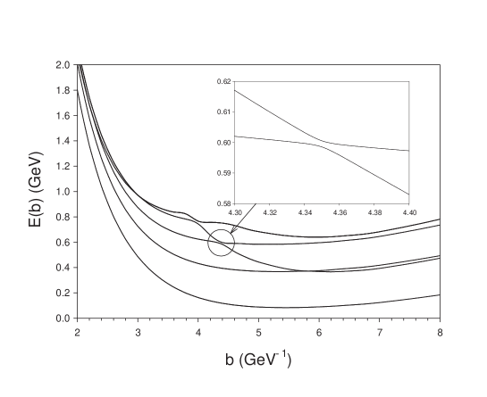
Figure 3: Binding energies of the five first $L=4$ $S=1/2$ $ubb$ baryon states for the potential of Bhaduri et al. bhad81 , as a function of the unique oscillator length $b$, for a number of quanta $N_{Q}=8$.

It is worth mentioning a phenomenon which can complicate the search of an optimal upper bound. On Fig. 3, the five first binding energies of a very asymmetric baryon are plotted as a function of an unique oscillator length $b$. At a first glance, one can see several crossings of levels for particular value of $b$. If we zoom on these points, we can see that there is no crossing at all actually. We have remarked that the apparition of (what we call) pseudo-crossing is favoured for very asymmetric systems, high angular momenta and semirelativistic kinematics. It is worth noting that the value of $b$, for which a pseudo-crossing between two given levels appears, decreases when the number $N_{Q}$ of quanta increases. Indeed, when $N_{Q}$ increases, a wider range of values of $b$ allows to obtain a good approximation of the wave functions; the unphysical characteristics of the spectrum are rejected toward zero length parameter. Similar phenomena appears when two oscillator lengths are considered, but they are much more difficult to visualize. Sometimes, the presence of pseudo-crossings can perturb the search of a minimum since the binding energy can vary abruptly with the length parameter at these points. The solution is simply to take smaller ranges of $b$ values to search for the minimum energy.

V Conclusions

The quantum three-body problem is well under control from the numerical point of view. In this paper we have revisited the method based on an expansion of the wave function on HO basis. The advantage of this approach is the possibility to allow different sizes $b_{x}$ and $b_{y}$ for HO functions related to different Jacobi coordinates ${\bf x}$ and ${\bf y}$.

We proved that the matrix elements can be calculated without any approximation and exactly for any value of the number of quanta $N_{Q}$. The complications as compared to the traditional approach is that we are obliged now to perform a double minimization on $b_{x}$ and $b_{y}$ instead of a single minimization on an unique parameter $b$; moreover the Brody-Moshinsky coefficients need also to be recalculated each time we change the size parameters. These disagreements are largely compensated by the fact that, for a given precision, the matrices to be diagonalized are much smaller. This last point is equivalent to say that for a given number of quanta, the precision achieved can be largely increased as compared to the old method. We thus think that our new treatment is a good compromise between precision and numerical effort.

Since it is universal and systematic, our method is particularly well suited for very asymmetric systems (for example one light and two heavy particles) and for systems having a large orbital angular momentum ($L$ = 4, 5, 6, …). This is not the case for most of other competitive approaches. Moreover, the method works particularly well for semirelativistic kinematics. We have been very careful to include several options (storage of BMC, use of Talmi’s integrals, special minimization procedure, …) that allow a drastic gain in computer time. The numerical code can be adapted on any normal personal computer and the results are already very satisfactory even with a few tens of seconds run on these machines.

Besides the numerical aspect, which is however very important, this method deals with more appropriate degrees of freedom and thus sticks more to the physical system. In particular a good precision can be achieved with a wave function containing a quite reasonable number of basic states $N$. This point is very important for the calculation of physical observables which grows as $N^{2}$.

For the moment our code can deal with nonrelativistic and semirelativistic kinetic energy terms and with central and hyperfine potentials. It can be adapted, with some modifications, to treat also more complex structures such as instanton effects, spin-orbit and tensor forces. The treatment of three-body interaction can also be considered. Some of these aspects are already under work.

Appendix A Talmi’s integrals

The computation of matrix elements (7) can be performed in a very efficient way by means of the so-called Talmi’s integrals. It can be shown that bro

$$V_{nl,n^{\prime}l^{\prime}}(b)=\delta_{ll^{\prime}}\sum_{p=l}^{n+n^{\prime}+l}B(n,n^{\prime},l,p)\>I_{p}(V,b).$$ (35)

In presence of tensor forces, formula (35) must be modified as states with different orbital angular momenta are mixed. In this case, new coefficients $B(n,l,n^{\prime},l^{\prime},p)$ must be used. In expression (35), the quantities $B(n,n^{\prime},l,p)$ are geometrical coefficients which can be calculated once for all, while the numbers $I_{p}(V,b)$ are the Talmi’s integrals which must be computed each time the length scales of the HO functions are changed. They are explicitly given by the following formula

$$I_{p}(V,b)=\frac{2}{\Gamma(p+3/2)}\int_{0}^{\infty}x^{2p+2}\>\exp(-x^{2})\>V(bx)\>dx.$$ (36)

This method has two great advantages: i) only $2N+1$ Talmi’s integrals are necessary to get the $N(N+1)/2$ matrix elements, which save a lot of computation time; ii) most of the $I_{p}(V,b)$ quantities are given by an analytical expression, so that the complete set of matrix elements are obtained fast and with a good precision.

It is worth mentioning that the coefficients $B(n,n^{\prime},l,p)$ can be stored in such a way that the elements needed in a summation where they appear are placed contiguously in a one dimensional array so that the summation is restricted to a reading in sequence which is very fast. These coefficients can be computed very accurately but their values increase rapidly with the quantum numbers. As the summation (35) is an alternate one, the values of the Talmi’s integrals result from differences of large numbers. Working with double precision numbers limits the use of this technique for values of $n+n^{\prime}+l$ below a number around 20.

Some Talmi’s integrals for various potentials are given in Ref. sema97 . For the nonrelativistic kinetic energy term, it is not necessary to use Talmi’s integral since the matrix elements of p² on HO functions are very simple expressions (see formula (18)). The analytical form for the matrix elements of the semirelativistic kinetic energy operator (20) involves the calculation of the following Talmi’s integral

$$I_{p}\left(e^{-ax^{2}}\sqrt{bx^{2}+c}\right)=\sqrt{b}\left(\frac{c}{b}\right)^{p+2}U\left(p+\frac{3}{2},p+3,\frac{(1+a)c}{b}\right).$$ (37)

$U(x,y,z)$ is a Kummer function abra70 , which can be calculated accurately by using recurrence formula for small values of $z$, or asymptotic expansion for large values of $z$. For medium values of this parameter, a direct integration of (36), by Gauss-Laguerre method for instance, gives the best accuracy.

Appendix B Minimization procedure

For a given number of quanta, the quality of the lower bound $E_{k}$ for the $k$th level depends on the length scales parameters $b_{x}$ and $b_{y}$. As we have seen in Sec. II.5, only one parameter $b$ is relevant in the case of three identical parameters. It is then necessary to find a fast method to compute the minimum of the functions $E_{k}(b_{x},b_{y})$ or $E_{k}(b)$. Let us focus first on the case of one nonlinear parameter.

A very efficient algorithm to find the minimum of a one parameter function is the Brent’s method pres92 . It relies on successive approximations of the function by parabolic curves. This method is robust and necessitates only the computation of one new point at each iteration, but it presents 3 drawbacks: i) to start, three abscissas must be given in a such way that the second one corresponds to the lowest ordinate; ii) nothing prevents the algorithm to find a new abscissa with a value irrelevant for the problem chosen; iii) the real form of the function can be very different of a parabola in the first steps of the procedure, which can increases dramatically the computation time. A way to cure simultaneously these flaws is to approach the function to minimize, at least for the first iterations, by a trial function presenting one minimum and which matches at best the real functions in the relevant range of abscissa values. In order to not penalize the method, the trial function must be defined with only three parameters as a parabola. One can try

$$y=\alpha x^{m}+\beta x^{n}+\gamma x^{p},$$ (38)

where $m$, $n$ and $p$ are different fixed real numbers. Given 3 values $y_{1}$, $y_{2}$ and $y_{3}$, for 3 given values $x_{1}$, $x_{2}$ and $x_{3}$, the parameters $\alpha$, $\beta$ and $\gamma$ can be found analytically if one power vanishes or if $n=(m+p)/2$. So we always work with these constraints.

Applied to the study of baryons with nonrelativistic kinematics for instance, we found that the choice $m=-2$, $n=1$ and $p=0$ allows a fast computation of the minimum of the curve $E_{k}(b)$, even if the position of the minimum is very badly estimated. These numbers stems from the dependence on $b$ of the Talmi’s integral. Other sets of numbers can be easily found in the case of different interactions.

To search the minimum of the functions $E_{k}(b_{x},b_{y})$, we apply our modified Brent’s method alternatively for parameters $b_{x}$ and $b_{y}$. With a judicious management of the search procedure, this method is in most cases faster and safer than more sophisticated algorithms.

Table 1: Number of Brody-Moshinsky coefficients (BMC) to be calculated for a given number of quanta $N_{Q}$. For details concerning the algorithm, see for example Ref. sil85 .

$N_{Q}$	Number of BMC	$N_{Q}$	Number of BMC
0	1
1	5	9	12 225
2	24	10	22 352
3	80	11	39 136
4	240	12	66 168
5	616	13	108 264
6	1 456	14	172 320
7	3 144	15	267 312
8	6 389	16	405 537

Table 2: Binding energies $E$ (in MeV) of two lowest state $I=S=1/2$ baryons for the potential of Bhaduri et al. bhad81 . Energies are calculated with 16 quanta for values of oscillator parameters (in GeV^-1) which give the lowest energy for $N^{\prime}_{Q}$ quanta.

	$uuu$, $L=0$		$ubb$, $L=4$
$N^{\prime}_{Q}$	$b$	$E$	$b_{x}$	$b_{y}$	$E$
0	3.337	17.956
2	3.238	17.466
4	2.941	16.167	1.739	2.711	55.558
6	2.817	15.695	1.759	2.668	55.535
8	2.648	15.117	1.704	2.474	55.422
10	2.551	14.822	1.719	2.348	55.368
12	2.425	14.495	1.654	2.236	55.319
14	2.347	14.345	1.699	2.110	55.290
16	2.251	14.262	1.619	2.041	55.278

Table 3: Binding energies (in MeV) of the center of gravity $N-\Delta$ for the nonrelativistic (NR) and semirelativistic (SR) Fulcher’s models fulc94 as a function of the number of quanta $N_{Q}$. Energies are computed with the value of the oscillator parameter $b$ (in GeV^-1) which gives the lowest bound for $8$ quanta. The dimension $D_{Q}$ of the basis for $N_{Q}$ quanta is also indicated. Note that values of the binding energies are very different for the two models since the mass of quark $u$ is 0.325 GeV for the NR model and 0.150 GeV for the SR model.

$N_{Q}$	$D_{Q}$	NR	SR
		$b=3.119$	$b=2.639$
8	70	244.35	799.85
10	112	244.28	799.56
12	168	244.17	798.61
14	240	244.14	798.45
16	330	244.11	798.11

Table 4: Binding energies (in GeV) of the lowest state $S=1/2$ $ubb$ baryon, for two values of $L$, for the nonrelativistic Fulcher’s models fulc94 , as a function of the number of quanta $N_{Q}$. Energies $E_{1}$ are computed with an unique value of the oscillator parameter $b$, while energies $E_{2}$ are computed with $b_{x}$ and $b_{y}$ not constrained by the relation (4). Energies are computed with values of the oscillator parameters (in GeV^-1) which give the lowest bound for $8$ quanta. The dimension $D_{Q}$ of the basis for $N_{Q}$ quanta is also indicated.

$N_{Q}$	$D_{Q}$	$E_{1}$	$E_{2}$
$L=0$		$b=3.592$	$b_{x}=0.996$
			$b_{y}=2.260$
8	35	0.3664	0.3661
10	56	0.3661	0.3659
12	84	0.3654	0.3654
14	120	0.3652	0.3652
16	165	0.3650	0.3650
$L=4$		$b=5.521$	$b_{x}=1.766$
			$b_{y}=2.565$
8	50	1.0929	1.0703
10	100	1.0783	1.0699
12	175	1.0732	1.0696
14	280	1.0713	1.0695
16	420	1.0705	1.0694

Table 5: Same as for Table 4 but for the semirelativistic Fulcher’s models fulc94 .

$N_{Q}$	$D_{Q}$	$M_{1}$	$M_{2}$
$L=0$		$b=3.951$	$b_{x}=0.963$
			$b_{y}=1.650$
8	35	0.6242	0.5969
10	56	0.6141	0.5966
12	84	0.6067	0.5948
14	120	0.6034	0.5945
16	165	0.6003	0.5938
$L=4$		$b=6.667$	$b_{x}=1.651$
			$b_{y}=2.147$
8	50	1.5441	1.3603
10	100	1.4729	1.3591
12	175	1.4304	1.3578
14	280	1.4045	1.3573
16	420	1.3885	1.3569

Table 6: Binding energies $E$ (in GeV) of the lowest state $L=4$ $S=1/2$ $ucb$ baryon for the semirelativistic Fulcher’s models fulc94 , as a function of the number of quanta $N_{Q}$, and as a function of the coupling mode between particles. Energies are computed with $b_{x}$ and $b_{y}$ optimum for $N^{\prime}_{Q}$ quanta. The dimension $D_{Q}$ of the basis for $N_{Q}$ quanta is also indicated.

		$c[ub]$			$u[cb]$
$N^{\prime}_{Q}$	$N_{Q}$	$D_{Q}$	$b_{x}$	$b_{y}$	$E$	$b_{x}$	$b_{y}$	$E$
4	4	10	2.635	2.112	1.7394	2.131	2.442	1.6915
6	6	40	2.646	2.087	1.6833	2.115	2.469	1.6718
8	8	100	2.553	2.064	1.6638	2.091	2.343	1.6587
8	10	200			1.6587			1.6566
8	12	350			1.6562			1.6550
8	14	560			1.6553			1.6545
8	16	840			1.6546			1.6541

Table 7: Masses (in GeV) of some $L=0$ baryons for the nonrelativistic (NR) and semirelativistic (SR) Fulcher’s models fulc94 , compared with experiment (Exp.). All values given are masses relieved of chromomagnetic contribution (see text). The value of the corrective term is given for both model, as well as the corresponding $\chi^{2}$ values.

Baryons	Exp.	NR	SR
$N-\Delta$ ($1S$)	1.086	1.086	1.086
$N-\Delta$ ($2S$)	1.520	1.827	1.655
$\Lambda-\Sigma-\Sigma^{*}$ ($1S$)	1.269	1.250	1.269
$\Lambda-\Sigma-\Sigma^{*}$ ($2S$)	1.735	1.928	1.832
$\Xi-\Xi^{*}$ ($1S$)	1.439	1.437	1.455
$\Omega$ ($1S$)	1.611	1.660	1.679
$\displaystyle{\frac{A}{m_{1}m_{2}m_{3}}}$ (GeV)		$-0.133$	$-0.162$
$\chi^{2}$		$119.4$	$28.5$

Figure 2: Regge trajectories for the positive parity $I=3/2$ baryons. Circle indicates the experimental values with the error bars. Solid (dashed) line joins the theoretical values from the semirelativistic (nonrelativistic) Fulcher’s model fulc94 .

References

- (1) J. Carlson, Phys. Rev. C 36, 2026 (1987).
- (2) W. von der Linden, Phys. Rep. 220, 53 (1992).
- (3) B. L. Hammond et al., Monte Carlo methods in Ab initio quantum chemestry (World Scientific, Singapore, 1994).
- (4) W. Glöckle, The quantum mechanical few-body systems (Springer Verlag, Berlin, Heidelberg, 1983).
- (5) M. Fabre de la Ripelle, Ann. Phys. 147, 281 (1983).
- (6) Y. Suzuki and K. Varga, Stochastic variational approach to quantum mechanical few-body problems (Springer Verlag, Berlin, Heidelberg, 1998).
- (7) N. Isgur and G. Karl, Phys. Rev. D 18, 4187 (1978). N. Isgur and G. Karl, Phys. Rev. D 20, 1191 (1979).
- (8) B. Silvestre-Brac, Few-Body Systems 20, 1 (1996).
- (9) R. D. Lawson, Theory of the nuclear shell model (Oxford University Press, 1980).
- (10) T. A. Brody and M. Moshinsky, Tables of transformation brackets (Monografias del Instituto de Fisica,Mexico, 1960).
- (11) B. Silvestre-Brac, J. Physique 46, 1087 (1985).
- (12) C. Semay and B. Silvestre-Brac, Phys. Rev. D 51, 1258 (1995).
- (13) R. K. Bhaduri, L. E. Cohler, and Y. Nogami, Nuovo Cimento 65A, 376 (1981).
- (14) Lewis P. Fulcher, Phys. Rev. D 50, 447 (1994).
- (15) S. Godfrey and N. Isgur, Phys. Rev. D 32, 189 (1985); S. Capstick and N. Isgur, Phys. Rev. D 34, 2809 (1986); L. Ya. Glozman et al., Phys. Rev. C 57, 3406 (1998); L. Ya. Glozman, W. Plessas, K. Varga, and R. F. Wagenbrunn, Phys. Rev. D 58, 094030 (1998).
- (16) F. E. Close, An Introduction to Quarks and Partons (Academic Press, 1979).
- (17) C. Semay and B. Silvestre-Brac, Nucl. Phys. A 618, 455 (1997).
- (18) M. Abramowitz and I. A. Stegun, Handbook of mathematical functions (Dover publications, Inc., New York, 1970).
- (19) William H. Press, Saul A. Teukolsky, William T. Vetterling, and Brain P. Flannerey, Numerical Recipes in FORTRAN (Cambridge University Press, 1992).