Large-Scale Zone-Based Evacuation Planning:
Models, Algorithms, and Evaluation

Abstract

In zone-based evacuation planning, the region to evacuate is divided into zones and each zone must be assigned a path to safety and departure times along the path. Zone-based evacuations are highly desirable in practice because they allow emergency services to communicate evacuation orders and to control the evacuation more accurately. Zone-based evacuations may also be combined with contraflows (to maximize the network capacities) and may impose additional constraints on the evacuation path (e,g,. path convergence) and the departure times (e.g., non-preemption).

This paper presents a systematic study large-scale zone-based evacuation planning, both from an effectiveness and a computational standpoint. It reviews existing optimization algorithms, and presents new ones, and evaluates them, on a real, large-scale case study, both from a macroscopic standpoint and through microscopic simulations under a variety of assumptions. The results provide some unique perspectives on the strengths and weaknesses of each approach and the implications of evacuation functionalities. The paper also suggests new directions for future research in zone-based evacuation and beyond in order to address the fundamental challenges by emergency services around the world.

1 Introduction

Large-scale evacuations are often necessary and critical to the preservation of safety and lives of residents in regions threatened by man-made or natural disasters like floods, hurricanes, and wildfires. According to a report by the International Federation of Red Cross and Red Crescent Societies [35], the first decade of the 21^st century witnessed 7184 disasters around the world which affected a total of 2.55 billion people, accounted for the deaths of more than 1 million people, and incurred $986 billion in economic losses. There is now an evacuation of 1,000 or more people every two or three weeks in the United States alone.

Effective disaster management requires, among others, evacuation plans that ensure resources like transportation network capacity and time are not completely overwhelmed by evacuee demand. Traffic congestion and associated delays which usually result from self-evacuations, in which individuals are given the freedom to choose their own evacuation routes, destinations, and times, significantly increase the risk of casualties being stranded in disaster affected areas. Therefore, it is crucial for emergency authorities to be equipped with centralized disaster management tools capable of generating and prescribing plans that guarantee optimal utilization of evacuation resources to attain specific goals like maximizing the number of evacuees reaching safety or minimizing overall evacuation time. Evacuation planning algorithms fulfill this need by producing prescriptive evacuation plans, i.e., a set of operational instructions for authorities to manage and orchestrate large-scale evacuations through the specification of directions for evacuees, including routes from their homes to designated safe destinations and departure times to be followed, as well as identification of roads that need to be closed to facilitate traffic flow. This contrasts to self-evacuations that are more difficult to control and may produce significant congestion.

Hamacher and Tjandra [16] distinguish between microscopic and macroscopic approaches to evacuation modeling. Microscopic approaches model individual characteristics of evacuees, their interactions with each other, and how these factors influence their movement. In contrast, macroscopic approaches aggregate evacuees and model their movements as flow in a network, making them much more amenable to optimization. Macroscopic models are often defined in terms of flows over time in order to capture capacity constraints more accurately. In particular, they typically use the concept of time-expanded graphs pioneered by Ford and Fulkerson [13].

This study is concerned with macroscopic approaches to prescriptive evacuation planning, although all results are validated using microscopic traffic simulations. Moreover, it focuses on zone-based evacuations in which all evacuees from the same residential zone are assigned a single evacuation route. Most emergency services rely on zone-based evacuations which facilitate the communication of evacuation plans, reduce confusion, increase compliance, and allow for a more reliable control of the evacuation Indeed, zone-based evacuations are probably the only practical method for communicating instructions precisely to the population at risk. They are however much more computationally challenging to plan and finding scalable algorithms has been one of the foci of recent research.

The core Zone-based Evacuation Planning Problem (ZEPP) considered in this study consists in assigning an evacuation path, as well as departure times, to each zone in the region. However, even when restricting attention to zone-based evacuations, several important design decisions remain to be taken: They include, but are not limited to, contraflows, convergent plans, and preemption.

• Contraflows, also known as lane reversals, are the idea of using inbound lanes for outbound traffic in evacuations. Several studies have suggested contraflow procedures as a viable method for increasing network capacity (e.g., [39, 37]).

• Convergent plans ensure that each evacuee coming to an intersection follows the same path subsequently. The rationale for convergent plans is that they eliminate forks from all evacuation paths and hence reduce driver hesitation at road intersections, which has been shown to be a significant source of delays [38]. Convergent paths also allow roads which are not part of the evacuation paths to be blocked, facilitating vehicular guidance and enforcement of the evacuation plans.

• Non-preemptive evacuations ensure that the evacuation of a zone, once it starts, proceeds without interruptions. Non-preemptive evacuations are also preferred by emergency services since they are easier to enforce.

Each of these decisions has a significant impact, not only on the effectiveness of an evacuation (e.g., the number of evacuees reaching safety), but also on the computational properties of the optimization model and its potential solution techniques.

The purpose of this paper is to provide a systematic comparative study of zone-based evacuation planning, their design choices, their fidelity, and their computational performance. It synthesizes existing algorithms, complements them with some new ones to fill some of the gaps in the design space, and compares them on a real-life case study both at macroscopic and microscopic scales. The case study concerns the the Hawkesbury-Nepean (HN) region located north-west of Sydney, Australia; The associated time-expanded graph has 30,000 nodes and 75,000 arcs.

The benefits of this study are threefold:

1. It systematically evaluates, on a large case study and for the first time, a variety of zone-based evacuation planning algorithms both from macroscopic and microscopic viewpoints;

2. It quantifies, for the first time, the benefits and limitations of contraflows, convergent plans, and preemption, providing unique perspectives on how to deploy these algorithms in practice;

3. It highlights the approaches that are best suited to capture each of these design features and the computational burden they impose.

4. It suggests potential directions for future research.

Finally, the paper addresses some other avenues for future research that are not satisfactorily addressed in the literature yet but are critical in practice.

The rest of this paper is organized as follows. Section 2 outlines the key concepts in zone-based evacuation planning, including time-expanded graphs, contraflows, and convergent evacuations. Section 3 provides a Mixed Integer Program (MIP) for non-convergent, preemptive evacuation planning with contraflows. This MIP introduces the main decision variables that appear in most approaches discussed in the paper. Section 4 presents a Benders Decomposition approach for non-convergent, preemptive ZEPP and Section 5 reviews the Benders decomposition approach for the convergent preemptive ZEEP originally proposed in [36]. Section 6 presents the conflict-based path-generation heuristic algorithm proposed in [34] for the non-convergent, preemptive ZEEP, while Section 7 reviews the column-generation approach to the non-convergent, non-preemptive ZEEP which was originally proposed in [33] and improved upon in [17]. Section 9 presents the case study, the experimental setting, and some initial observations. Section 10 presents the experimental results from a macroscopic standpoint and Section 11 provides the details of the microscopic simulations. Section 12 gives some perspectives on directions for future research and knowledge gaps that needs to be filled. Section 13 discusses some related work to give more context to all the results in the paper. Finally, Section 14 concludes the paper.

2 Problem Formulation

Figure 1 shows an example of the evacuation scenario that is addressed by all methods presented in this work. Square 0 represents an evacuation node (e.g., a residential zone), triangles A and B represent safe nodes (final evacuation destinations), circles 1-3 represent transit nodes (road intersections), and arcs represent roads connecting the nodes. Times on each arc indicate when each road will become unavailable (e.g., due to being flooded) and the time on the evacuation node indicates the final deadline by which it must be evacuated. In this example, the evacuation deadline for node 0 is 13:00 since its last outgoing arc will be blocked at that time.

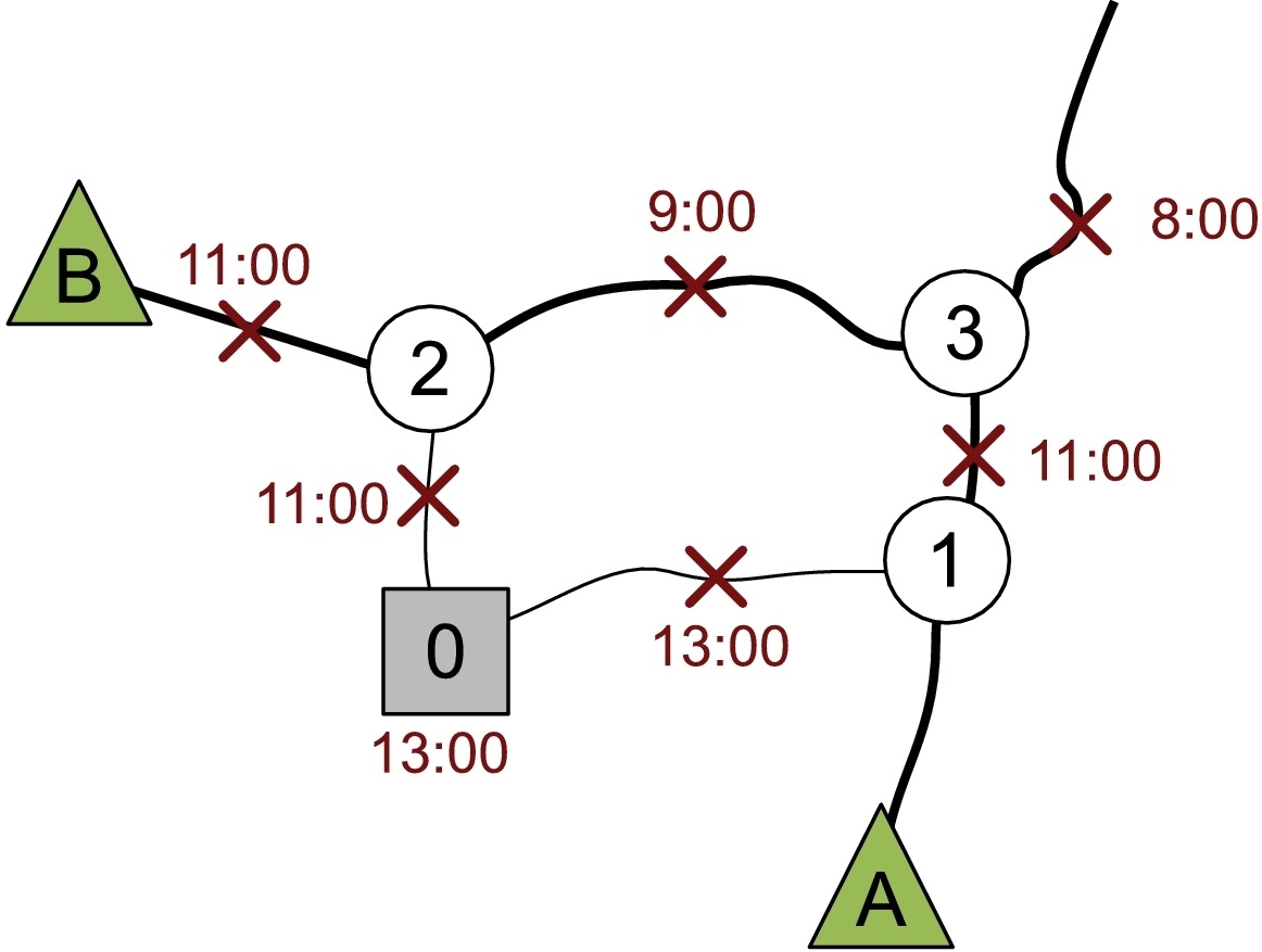
Figure 1: A Sample Evacuation Scenario.

The evacuation scenario can be abstracted by a static evacuation graph $\mathcal{G}=(\mathcal{N}=\mathcal{E}\cup\mathcal{T}\cup\mathcal{S},\mathcal{A})$ where $\mathcal{E}$, $\mathcal{T}$, and $\mathcal{S}$ are the set of evacuation, transit, and safe nodes respectively, and $\mathcal{A}$ is the set of all arcs. Each evacuation node $k\in\mathcal{E}$ has associated with its demand $d_{k}$ representing the number of vehicles to be evacuated and its evacuation deadline $f_{k}$, while each arc $e\in\mathcal{A}$ has associated with its travel time $s_{e}$, its capacity $u_{e}$ in terms of vehicles per unit time, and its block time $f_{e}$ at which the road becomes unavailable. Figure 2 shows the static evacuation graph for the scenario of Figure 1. The evacuation node is labeled with its demand and evacuation deadline while the arcs are labeled with their travel time, capacity, and block time. Also note that the evacuation node has no incoming arcs and the safe nodes have no outgoing arcs.

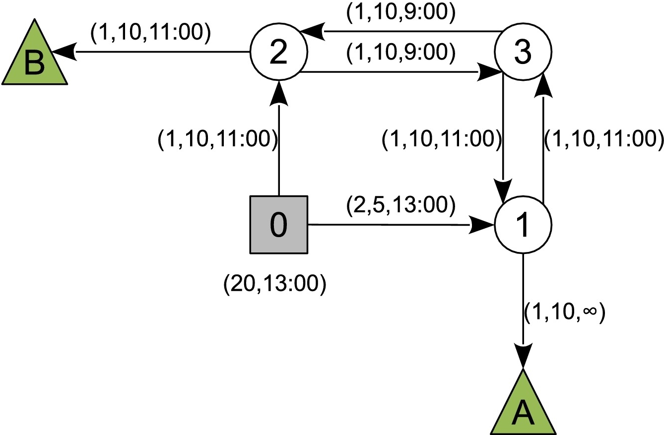
Figure 2: The Static Evacuation Graph for the Scenario in Figure 1.

In order to reason about traffic flows over time, the static graph is converted into a time-expanded graph $\mathcal{G}^{x}=(\mathcal{N}^{x}=\mathcal{E}^{x}\cup\mathcal{T}^{x}\cup\mathcal{S}^{x},\mathcal{A}^{x})$. The conversion is performed by first discretizing the time horizon $\mathcal{H}$ into time steps of identical length $t\in\mathcal{H}$, creating a copy of all nodes at each time step, and replacing each arc $e=(i,j)$ with corresponding arcs $e_{t}=(i_{t},j_{t+s_{e}})$ for each time step that $e$ is available. Figure 3 shows the time-expanded graph constructed from the static graph of Figure 2, where each arc is labeled with its capacity. Infinite capacity arcs are introduced connecting the evacuation and safe nodes at each time step to allow evacuees to wait at those nodes. Nodes that cannot be reached from either the evacuation or safe nodes within the time horizon are removed from the graph (they are greyed out in Figure 3).

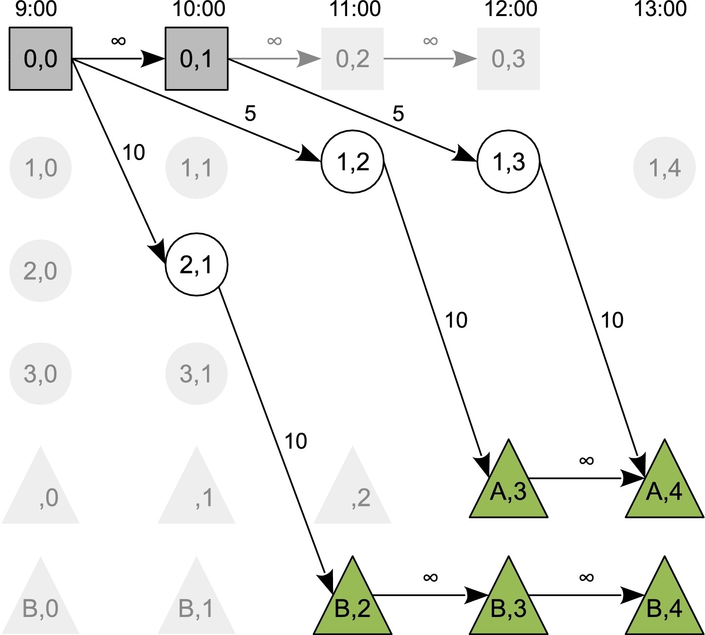
Figure 3: The Time-expanded Graph of Static Graph in Figure 2.

An evacuation plan can then be defined to contain the following two components: (a) a set of evacuation paths, each represented by a sequence of connected nodes in the static graph from an evacuation node to a safe node, specifying the route to be taken by residents of each evacuation node to reach safety, and (b) an evacuation schedule indicating the number of vehicles that need to depart from each evacuation node at each time step $t\in\mathcal{H}$. The Zone-Based Evacuation Planning Problem (ZEPP) can now be defined as follows.

Definition 1

Given an evacuation graph $\mathcal{G}$, the Zone-Based Evacuation Planning Problem (ZEPP) consists of finding an evacuation path from each evacuation zone to a safe node that maximize the flow of evacuees to safe nodes, while satisfying the problem constraints.

Contraflows

Contraflows are an important tool in evacuation planning and scheduling. To capture their benefits, this study assumes the existence of a subset $\mathcal{A}_{c}\subseteq\mathcal{A}$ of arcs in the static graph that may be used in contraflows during evacuations. The unique arc that goes in the opposite direction of arc $e\in\mathcal{A}_{c}$ is denoted by $\bar{e}$. The set $\mathcal{A}_{c}$ can then be partitioned into $\hat{\mathcal{A}}_{c}$ and $\check{\mathcal{A}}_{c}$ such that $\forall e\in\hat{\mathcal{A}}_{c}:\bar{e}\in\check{\mathcal{A}}_{c}$. Finally, $e_{0}\in\mathcal{A}$ denotes the static edge associated with edge $e\in\mathcal{A}^{\text{x}}$ and $\delta^{-}(i)$ and $\delta^{+}(i)$ denote the set of incoming and outgoing arcs of node $i$ respectively.

Convergent Evacuations

Convergent paths reduce confusion and hesitation during an evacuation. They can be formally defined by the following definitions.

Definition 2

A graph $\mathcal{G}=(\mathcal{N},\mathcal{A})$ is connected if, for all $k\in\mathcal{E}$, there exists a path from $k$ to a safe node.

Definition 3

A graph $\mathcal{G}=(\mathcal{N},\mathcal{A})$ is convergent if, for all $i\in\mathcal{E}\cup\mathcal{T}$, the outdegree of $i$ is $1$.

As stated by [12], any connected evacuation graph $\mathcal{G}$ contains a connected and convergent subgraph $\mathcal{G}^{\prime}$. If an evacuation graph is connected and convergent, each evacuation node has a unique path to a safe node. The Convergent Zone-Based Evacuation Planning Problem (C-ZEPP) is defined as follows:

Definition 4

Given a connected evacuation graph $\mathcal{G}$, the Convergent Zone-Based Evacuation Planning Problem (C-ZEPP) consists of finding a convergent subgraph $\mathcal{G}^{\prime}$ of $\mathcal{G}$ and a set of evacuee departure times that maximize the flow from evacuation nodes to safe nodes, while satisfying the problem constraints.

Non-Preemption and Response Curves

Non-preemptive evacuation plans are typically organized around the concept of response curves [32]. A response curve $f$ is a function that models the number of evacuees departing an evacuation node over time after an evacuation start time $t_{0}\in\mathcal{H}$. The number $D_{k}(t)$ of evacuees departing an evacuation node $k$ at time $t$ is defined using a selected response curve $f$ as follows:

$$D_{k}(t)=\begin{cases}0&\text{if}\ t<t_{0}\\ f(t-t_{0})&\text{if}\ t\geq t_{0}\end{cases}$$ (1)

$D_{k}(t)$ can be used to precisely specify a non-preemptive evacuation schedule for evacuation node $k$. Figure 4 shows $D_{k}(t)$ utilizing four different types of response curves. The S-shape, Rayleigh and inverse Rayleigh curves use $t_{0}$ = 60 minutes, while the step function uses $t_{0}$ = 120 minutes. The step response curve, where evacuees depart at a constant rate after $t_{0}$ until a region is completely evacuated, is the response curse considered in this paper.

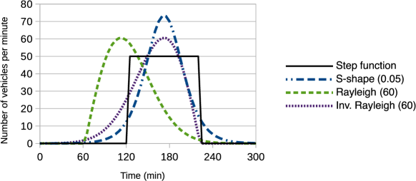
Figure 4: The number of evacuees departing an evacuation node $k$ as a function of time, $D_{k}(t)$, using four different types of response curves (from [33]).

Definition 5

Given an evacuation graph $\mathcal{G}$, the Non-Preemptive Zone-Based Evacuation Planning Problem (NP-ZEPP) consists of finding for each evacuation zone an evacuation path to a safe node, a departure time, and a response curve that maximize the flow of evacuees to safe nodes, while satisfying the problem constraints.

The paper considers the ZEPP, C-ZEPP, and NP-ZEPP problems and algorithms to solve them. Each of these problems is considered with and without contraflows.

3 The Basic MIP Model for the ZEPP

This section presents a Mixed Integer Program (MIP) model for the ZEPP. Model (2-11) in Figure 5 provides the intuition that serves as the basis for the more complex models presented subsequently. The decision variables of the model are as follows: Binary variable $x_{{e},{k}}$ is equal to 1 if and only if edge $e\in\mathcal{A}$ belongs to the evacuation path for evacuation node $k$, and $\varphi_{{e},{k}}$ is a continuous variable equal to the flow of evacuees from evacuation node $k$ on edge $e\in\mathcal{A}^{\text{x}}$. To indicate which road should be used in contraflows, binary variable $y_{e}$ represents whether arc $e$ is used in its normal direction ($y_{e}=1$) or in contraflow ($y_{e}=0$). Each road segment $(e,\bar{e})$ with $e\in\hat{\mathcal{A}}_{c},\bar{e}\in\check{\mathcal{A}}_{c}$ can then be utilized in one of three possible configurations: (a) $(y_{e},y_{\bar{e}})=(1,1)$ where both arcs are used in their normal directions, (b) $(y_{e},y_{\bar{e}})=(1,0)$ where arc $\bar{e}$ is used in contraflow, or (c) $(y_{e},y_{\bar{e}})=(0,1)$ where arc $e$ is used in contraflow.

$$\max\quad \sum_{k\in\mathcal{E}^{\text{x}}}\sum_{e\in\delta^{-}(v_{t})}\varphi_{{e},{k}}$$ (2)

s.t. $$\sum_{e\in\delta^{+}(k)}x_{{e},{k}}=1 \forall k\in\mathcal{E}$$ (3)

$$\sum_{e\in\delta^{-}(i)}x_{{e},{k}}-\sum_{e\in\delta^{+}(i)}x_{{e},{k}}=0 \forall k\in\mathcal{E},i\in\mathcal{T}$$ (4)

$$\sum_{e\in\delta^{-}(i)}\varphi_{{e},{k}}-\sum_{e\in\delta^{+}(i)}\varphi_{{e},{k}}=0 \forall i\in\mathcal{N}^{\text{x}}\setminus\{v_{s},v_{t}\},k\in\mathcal{E}$$ (5)

$$\sum_{k\in\mathcal{E}}\varphi_{{e},{k}}\leq u_{e} \forall e\in\mathcal{A}^{\text{x}}\setminus\mathcal{A}_{c}$$ (6)

$$\sum_{k\in\mathcal{E}}\varphi_{{e},{k}}\leq y_{{e_{0}}}u_{{e}}+(1-y_{{\bar{e_{0}}}})u_{{\bar{e}}} \forall e\in\mathcal{A}_{c}$$ (7)

$$\varphi_{{e},{k}}\leq u_{e}*x_{{e},{k}} \forall e\in\mathcal{A}^{\text{x}},k\in\mathcal{E}$$ (8)

$$y_{{e}}+y_{{\bar{e}}}\geq 1 \forall e\in\hat{\mathcal{A}}_{c}$$ (9)

$$y_{{e}}\in\{0,1\} \forall e\in\mathcal{A}_{c}$$ (10)

$$\varphi_{{e},{k}}\geq 0,x_{{e},{k}}\in\{0,1\} \forall e\in\mathcal{A}^{\text{x}},k\in\mathcal{E}$$ (11)

Figure 5: The MIP Model for the ZEEP.

Constraints (3) ensure that exactly one path is used to route the flow coming from evacuation nodes, while constraints (4) ensure the continuity of the path. Constraints (5) ensure flow conservation through the time-expanded graph. Constraints (6) enforce the capacity of each edge in the time-expanded graph. Constraints (7) enforce the capacity on edges that allow contraflow: They allocate to $e$ the capacity of edge $\bar{e}$ whenever $\bar{e}$ is used in contraflow, and forbid any flow on $e$ when it is used in contraflow. Constraints (8) ensure that there is no flow of evacuees coming from an evacuation node $k$ if edge $e$ is not part of the evacuation path for $k$. Constraints (9) prohibit the simultaneous use of $e$ and $\bar{e}$ in contraflow. The objective (2) maximizes the number of evacuees reaching safety.

Model (2-11) is intractable for the case study used in this paper which has approximately 30,000 nodes and 75,000 arcs. The computational difficulty comes from two interconnected components: The selection of the paths is a design component, while the scheduling of the evacuation is multi-commodity flow. The algorithms described in this paper address this computational challenge by separating these two aspects. Observe also that the temporal aspects (i.e., when to schedule evacuees along a path) are an important and difficult aspect of the ZEPP. Finally, it is interesting to mention that additional requirements, such as convergent evacuations and non-preemption, may lead to elegant computational contributions that would not be possible otherwise.

4 Benders Decomposition for the ZEEP

This section presents an (approximate) Benders decomposition for the ZEEP. This Benders decomposition is referred to as the Benders Non-convergent (BN) method in the rest of the paper. The Restricted Master Problem (RMP) of the Benders decomposition selects evacuation paths that are then used in the subproblem (SP) for scheduling the flows of evacuees over time along these paths. It is important to note that the subproblem is a multi-commodity flow and hence it is not totally unimodular. As a result, the Benders decomposition in the BN method solves a relaxation of the ZEEP where the integrality constraints on flow variables are relaxed. A final MIP is solved to obtain an integer solution to the subproblem.

As is traditional in Benders decomposition, the objective values of the RMP and SP provide upper and lower bounds on the optimal solution to Model (2-11) without integrality constraints on the flow variables. When they converge, evacuation paths from the RMP and the evacuation schedule from the SP form an optimal solution. Otherwise, a Benders cut is generated from the solution of the SP and introduced into the RMP as an additional constraint to remove the current evacuation paths from the RMP’s feasible region, after which the entire process is repeated.

The Restricted Master Problem

The RMP, depicted in Figure 6, finds evacuation paths for each evacuation zone. It operates on the static graph and its main decision variables are the binary variables $x_{e,k}$ of Model (2-11). In addition to the Benders cuts, the RMP also reasons about aggregate flows and aggregated capacities, an idea that was proposed in [36] to obtain reasonable evacuation paths early on. In particular, variable $\psi_{e,k}$ represents the aggregate flow of evacuees from evacuation node $k$ along arc $e$ and arc capacities are aggregated over the time horizon in all of the RMP’s capacity constraints. Finally, $z_{\text{RMP}}$ is the RMP’s objective value and represents the number of evacuees reaching safety.

$$\max z_{\text{RMP}}$$ (12)

subject to

$$z_{\text{RMP}}\leq\sum_{k\in\mathcal{E}}\sum_{e\in\delta^{+}(k)}\psi_{e,k}$$ (13)

$$\sum_{e\in\delta^{+}(k)}x_{e,k}=1\qquad\forall k\in\mathcal{E}$$ (14)

$$\sum_{e\in\delta^{+}(i)}x_{e,k}\leq 1\qquad\forall i\in\mathcal{T},\forall k\in\mathcal{E}$$ (15)

$$\sum_{e\in\delta^{-}(i)}\psi_{e,k}-\sum_{e\in\delta^{+}(i)}\psi_{e,k}=0\qquad\forall i\in\mathcal{T},\forall k\in\mathcal{E}$$ (16)

$$\sum_{e\in\delta^{+}(k)}\psi_{e,k}\leq d_{k}\qquad\forall k\in\mathcal{E}$$ (17)

$$\psi_{e,k}\leq x_{e,k}\sum_{t\in\mathcal{H}}u_{e_{t}}\qquad\forall e\in\mathcal{A}\setminus\mathcal{A}_{c},\forall k\in\mathcal{E}$$ (18)

$$\psi_{e,k}\leq x_{e,k}\sum_{t\in\mathcal{H}}(u_{e_{t}}+u_{\bar{e}_{t}})\qquad\forall e\in\mathcal{A}_{c},\forall k\in\mathcal{E}$$ (19)

$$\sum_{k\in\mathcal{E}}\psi_{e,k}\leq\sum_{t\in\mathcal{H}}u_{e_{t}}\qquad\forall e\in\mathcal{A}\setminus\mathcal{A}_{c}$$ (20)

$$\sum_{k\in\mathcal{E}}\psi_{e,k}\leq y_{e}\sum_{t\in\mathcal{H}}u_{e_{t}}+(1-y_{\bar{e}})\sum_{t\in\mathcal{H}}u_{\bar{e}_{t}}\qquad\forall e\in\mathcal{A}_{c}$$ (21)

$$y_{e}+y_{\bar{e}}\geq 1\qquad\forall e\in\mathcal{A}_{c}$$ (22)

$$\psi_{e,k}\geq 0\qquad\forall e\in\mathcal{A},\forall k\in\mathcal{E}$$ (23)

$$x_{e,k}\in\{0,1\}\qquad\forall e\in\mathcal{A},\forall k\in\mathcal{E}$$ (24)

$$y_{e}\in\{0,1\}\qquad\forall e\in\mathcal{A}_{c}$$ (25)

Figure 6: The Restricted Master Problem for the BN method.

Constraints (13), together with objective function (12), maximize the flow of evacuees from all evacuation nodes. Constraints (14) specify that exactly one path is generated for each evacuation node, and constraints (15) ensure that the one path requirement is preserved throughout the graph. Constraints (16) ensure that flow is conserved throughout the graph, and constraints (17) make sure that total flow from each evacuation node does not exceed its demand. Constraints (18) and (19) permit evacuee flow from evacuation node $k$ on an arc only if the arc is selected for the evacuation path of $k$. Constraints (20) ensure that the flow from all evacuation nodes along an arc does not exceed the aggregate capacity for arcs that may not be used in contraflow, while constraints (21) do the same for arcs that may be used in contraflow. Finally, constraints (22) indicate that at most one arc in road segment $(e,\bar{e})$ with $e\in\hat{\mathcal{A}}_{c},\bar{e}\in\check{\mathcal{A}}_{c}$ can be used in contraflow. To generate evacuation plans with contraflows, constraints (22) can be replaced with constraints

$$y_{e}+y_{\bar{e}}=2\qquad\forall e\in\mathcal{A}_{c}$$

which forces all arcs to be used in their normal directions.

The Benders Subproblem

The SP, depicted in Figure 7, utilizes paths generated from the RMP together with the time-expanded graph $\mathcal{G}^{x}$ to generate an evacuation schedule that maximizes the number of evacuees reaching safety along those paths. The paths are specified by the values $\{\bar{x}_{e,k}\}$ and $\{\bar{y}_{e}\}$ for variables $\{x_{e,k}\}$ and $\{y_{e}\}$ in the RMP. The SP uses variable $\varphi_{e_{t},k}$ to represent the flow of evacuees from evacuation node $k$ along arc $e_{t}$ in $\mathcal{G}^{x}$, and $z_{\text{SP}}$ is the SP’s objective value.

$$\max z_{\text{SP}}=\sum_{k\in\mathcal{E}}\sum_{e_{t}\in\delta^{+}(k)}\varphi_{e_{t},k}$$ (26)

subject to

$$\sum_{e_{t}\in\delta^{-}(i)}\varphi_{e_{t},k}-\sum_{e_{t}\in\delta^{+}(i)}\varphi_{e_{t},k}=0\qquad\forall i\in\mathcal{T}^{x},\forall k\in\mathcal{E}$$ (27)

$$\sum_{t\in\mathcal{H}}\sum_{e_{t}\in\delta^{+}(k)}\varphi_{e_{t},k}\leq d_{k}\qquad\forall k\in\mathcal{E}$$ (28)

$$\varphi_{e_{t},k}\leq\bar{x}_{e,k}\cdot u_{e_{t}}\qquad\forall e\in\mathcal{A}\setminus\mathcal{A}_{c},\forall t\in\mathcal{H},\forall k\in\mathcal{E}$$ (29)

$$\varphi_{e_{t},k}\leq\bar{x}_{e,k}\cdot(u_{e_{t}}+u_{\bar{e}_{t}})\qquad\forall e\in\mathcal{A}_{c},\forall t\in\mathcal{H},\forall k\in\mathcal{E}$$ (30)

$$\sum_{k\in\mathcal{E}}\varphi_{e_{t},k}\leq u_{e_{t}}\qquad\forall e\in\mathcal{A}\setminus\mathcal{A}_{c},\forall t\in\mathcal{H}$$ (31)

$$\sum_{k\in\mathcal{E}}\varphi_{e_{t},k}\leq\bar{y}_{e}\cdot u_{e_{t}}+(1-\bar{y}_{\bar{e}})\cdot u_{\bar{e}_{t}}\qquad\forall e\in\mathcal{A}_{c},\forall t\in\mathcal{H}$$ (32)

$$\varphi_{e_{t},k}\geq 0\qquad\forall e_{t}\in\mathcal{A}^{x},\forall k\in\mathcal{E}$$ (33)

Figure 7: The Bender Subproblem for the BN method.

The objective function (26) maximizes the flow of evacuees from all evacuation nodes. Constraints (27) enforce flow conservation throughout $\mathcal{G}^{x}$, while constraints (28) ensure that the total flow from each evacuation node does not exceed its demand. Constraints (29) and (30) permit flow only on the selected arcs for each evacuation node. Constraints (31) ensure that the total flow from all evacuation nodes along an arc does not exceed its capacity for arcs that may not be used in contraflow, while constraints (32) do the same for arcs that may be used in contraflow.

The Benders Cuts

A Benders optimality cut is generated from the solution of the SP and added to the RMP as long as the objective values of the RMP and SP do not converge. The cut is of the form

$$\begin{split}z_{\text{RMP}}\leq&\sum_{k\in\mathcal{E}}d_{k}\cdot\pi_{k}+\sum_{e\in\mathcal{A}\setminus\mathcal{A}_{c}}\sum_{t\in\mathcal{H}}u_{e_{t}}\sum_{k\in\mathcal{E}}x_{e,k}\cdot\pi_{e_{t},k}+\\ &\sum_{e\in\mathcal{A}_{c}}\sum_{t\in\mathcal{H}}(u_{e_{t}}+u_{\bar{e}_{t}})\sum_{k\in\mathcal{E}}x_{e,k}\cdot\pi_{e_{t,c},k}+\sum_{e\in\mathcal{A}\setminus\mathcal{A}_{c}}\sum_{t\in\mathcal{H}}u_{e_{t}}\cdot\pi_{e_{t}}+\\ &\sum_{e\in\mathcal{A}_{c}}\sum_{t\in\mathcal{H}}[y_{e}\cdot u_{e_{t}}+(1-y_{\bar{e}})\cdot u_{\bar{e}_{t}}]\cdot\pi_{e_{t,c}}\end{split}$$ (34)

where $\{\pi_{k}\}$, $\{\pi_{e_{t},k}\}$, $\{\pi_{e_{t,c},k}\}$, $\{\pi_{e_{t}}\}$, and $\{\pi_{e_{t,c}}\}$ are the dual variables of constraints (28), (29), (30), (31), and (32) respectively. Since the SP is always feasible, Benders feasibility cuts are never generated by this algorithm.

The Benders Non-convergent Algorithm

Algorithm 1 summarizes the entire BN algorithm which uses $\text{RMP}(\mathcal{G},\mathcal{H})$ to denote an optimal solution obtained from solving the RMP given static graph $\mathcal{G}$ and time horizon $\mathcal{H}$ as inputs, $\text{SP}(\Psi,\mathcal{H})$ to denote an optimal solution of the SP given a solution to the RMP, $\Psi$, and time horizon $\mathcal{H}$ as inputs, and $z(\sigma)$ to denote the objective value of a solution $\sigma$.

Algorithm 1 Benders Non-convergent

1:$t^{*}\leftarrow\min\{t\in\mathcal{H}\,|\,z(\text{RMP}(\mathcal{G},[0..t]))=z(\text{RMP}(\mathcal{G},\mathcal{H}))\}$

2:$z_{\text{RMP}}\leftarrow z(\text{RMP}(\mathcal{G},[0..t^{*}]))$

3:$z_{\text{SP}}\leftarrow z(\text{SP}(\text{RMP}(\mathcal{G},[0..t^{*}]),\mathcal{H}))$

4:$z_{\text{SP,max}}\leftarrow z_{\text{SP}}$

5:while $z_{\text{RMP}}-z_{\text{SP,max}}>\varepsilon$ do

6:     Generate Benders cut from solution of SP and add it to RMP

7:     $z_{\text{RMP}}\leftarrow z(\text{RMP}(\mathcal{G},\mathcal{H}))$

8:     $z_{\text{SP}}\leftarrow z(\text{SP}(\text{RMP}(\mathcal{G},\mathcal{H}),\mathcal{H}))$

9:     $z_{\text{SP,max}}\leftarrow\max\{z_{\text{SP,max}},z_{\text{SP}}\}$

10:Solve $\text{SP}(\text{RMP}(\mathcal{G},\mathcal{H}),\mathcal{H})$ with $\varphi_{e_{t},k}\ \text{integer}\ \forall e_{t}\in\mathcal{A}^{x},\forall k\in\mathcal{E}$

11:return Evacuation paths from solution of RMP and evacuation schedule from solution of SP

The BN algorithm begins with a procedure that searches for the tightest time horizon $t^{*}$ that can preserve the optimal solution to the RMP, $z(\text{RMP}(\mathcal{G},\mathcal{H}))$. This step was originally proposed by Even et al. [12] who found that a tighter time horizon produces better evacuation paths for the flow scheduling problem of their two-stage approach. The BN method adopts a similar strategy to seed the Benders decomposition. The procedure is implemented using a simple sequential search which solves $\text{RMP}(\mathcal{G},\mathcal{H})$ with progressively smaller values of $\mathcal{H}$ in search of $t^{*}$.

After this step, the algorithm proceeds to first solve the RMP to generate evacuation paths, and then the SP using the generated paths as input to generate an evacuation schedule. The minimum objective value $z_{\text{RMP}}$ of the RMP is then compared to the maximum objective value $z_{\text{SP,max}}$ of the SP. If they do not converge (if their difference is larger than a convergence criterion $\varepsilon$, which we set to 0), a Benders cut is generated utilizing dual variables from the solution of the SP and added to the RMP to remove the current evacuation paths from its feasible region. The process of solving the RMP and SP is then repeated until convergence. Since the Benders decomposition relaxes the integrality constraints on the flow variables, the subproblem is solved one more time as a MIP after convergence to obtain an integer solution to the subproblem.

5 Benders Decomposition for Convergent Evacuation Planning

This section present the Benders decomposition of [36] for the C-ZEEP, i.e., for the convergent preemptive zone-based evacuation planning. This Benders decomposition is referred to as the Benders convergent (BC) method in this paper. The BC method shares a lot of similarities with the BN method. The BC method however imposes that the evacuation paths form a convergent graph and hence that the outdegree at each transit node is at most 1. This convergence property has some fundamental consequences: (1) the BC method is exact since the subproblem becomes totally submodular; (2) it trivially supports contraflows; and (3) its computational performance is strong compared to all the other algorithms.

The Restricted Master Problem

$$\max z_{\text{RMP}}$$ (35)

subject to

$$z_{\text{RMP}}\leq\sum_{k\in\mathcal{E}}\sum_{e\in\delta^{+}(k)}\psi_{e}$$ (36)

$$\sum_{e\in\delta^{-}(i)}\psi_{e}-\sum_{e\in\delta^{+}(i)}\psi_{e}=0\qquad\forall i\in\mathcal{T}$$ (37)

$$\sum_{e\in\delta^{+}(i)}x_{e}\leq 1\qquad\forall i\in\mathcal{E}\cup\mathcal{T}$$ (38)

$$\psi_{e}\leq x_{e}\sum_{t\in\mathcal{H}}u_{e_{t}}\qquad\forall e\in\mathcal{A}$$ (39)

$$\sum_{e\in\delta^{+}(k)}\psi_{e}\leq d_{k}\qquad\forall k\in\mathcal{E}$$ (40)

$$\psi_{e}\geq 0\qquad\forall e\in\mathcal{A}$$ (41)

$$x_{e}\in\{0,1\}\qquad\forall e\in\mathcal{A}$$ (42)

Figure 8: The Restricted Master Problem for the BC method.

The RMP for the BC method is presented in Figure 8. Because the paths are convergent, the model is considerably simpler: There is no need to track the origin of the flow (i.e., the evaluation zone) and have different flow conservation constraints for each evacuation zone. The model still uses a binary variable $x_{e}$ to indicate if an arc $e$ is to be part of an evacuation path. But it uses a single variable $\psi_{e}$ to represent the aggregate flow of evacuees along arc $e$ over the time horizon. Arc capacities are again aggregated over the time horizon in the capacity constraints. Constraint (36) combined with objective function (35) maximizes the flow of evacuees leaving all evacuation nodes. Constraint (37) enforces flow conservation, while constraint (38) enforces the convergence of arcs selected by the evacuation paths. Constraints (39) permit flows only on selected arcs and ensures aggregate flow along them do not exceed their aggregate capacity. Finally, constraint (40) ensures that the total flow from each evacuation node does not exceed its demand.

The Benders Subproblem

The Benders problem for method BC, depicted in Figure 9, is again simpler due to path convergence and uses a a variable $\varphi_{e_{t}}$ to represent flow of evacuees along arc $e_{t}$ in $\mathcal{G}^{x}$. Objective function (43) maximizes flow of evacuees across all evacuation nodes. Constraints (44) enforce flow conservation, constraints (45) permit flow only on arcs selected for evacuation paths and ensure the flow does not exceed the arc’s capacity, and constraints (46) ensure that the total flow leaving each evacuation node does not exceed its demand.

$$\max z_{\text{SP}}=\sum_{k\in\mathcal{E}}\sum_{e_{t}\in\delta^{+}(k)}\varphi_{e_{t}}$$ (43)

subject to

$$\sum_{e_{t}\in\delta^{-}(i)}\varphi_{e_{t}}-\sum_{e_{t}\in\delta^{+}(i)}\varphi_{e_{t}}=0\qquad\forall i\in\mathcal{T}^{x}$$ (44)

$$\varphi_{e_{t}}\leq\bar{x}_{e}\cdot u_{e_{t}}\qquad\forall e\in\mathcal{A},\forall t\in\mathcal{H}$$ (45)

$$\sum_{e_{t}\in\delta^{+}(k)}\varphi_{e_{t}}\leq d_{k}\qquad\forall k\in\mathcal{E}$$ (46)

$$\varphi_{e_{t}}\geq 0\qquad\forall e_{t}\in\mathcal{A}^{x}$$ (47)

Figure 9: The Bender Subproblem for the BN method.

The Benders Cuts

The Benders optimality cuts are of the form

$$z_{\text{RMP}}\leq\sum_{e\in\mathcal{A}}x_{e}\sum_{t\in\mathcal{H}}u_{e_{t}}\cdot\pi_{e_{t}}+\sum_{k\in\mathcal{E}}d_{k}\cdot\pi_{k}$$ (48)

and use dual variables $\{\pi_{e_{t}}\}$ and $\{\pi_{k}\}$ associated with constraints (45) and (46) of the SP respectively. Again, Benders feasibility cuts are never generated in this algorithm because the SP is always feasible.

Pareto-Optimal Cuts

The convergence of Benders decomposition can be accelerated through utilization of Pareto-optimal cuts [36], i.e., cuts that are not dominated by any other Benders cut. The Magnanti-Wong method [30] is utilized to generate these stronger cuts. The method requires a core point, i.e., a point located within the relative interior of the convex hull of the feasibility domain of the RMP’s first-stage variable $\{x_{e}\}$. For this formulation, the core point utilized is simply $x_{e}^{0}=\frac{1}{|\delta^{+}(i)+1|}$ for each arc $e=(i,j)$. The dual of the Magnanti-Wong problem (DMWP) which utilizes this core point and the optimal objective value of the SP, $z_{\text{SP}}$, is solved to generate a Pareto-optimal cut.

$$\max\sum_{k\in\mathcal{E}}\sum_{e_{t}\in\delta^{+}(k)}\varphi_{e_{t}}+\xi\cdot z_{\text{SP}}$$ (49)

subject to

$$\sum_{e_{t}\in\delta^{-}(i)}\varphi_{e_{t}}-\sum_{e_{t}\in\delta^{+}(i)}\varphi_{e_{t}}=0\qquad\forall i\in\mathcal{T}^{x}$$ (50)

$$\varphi_{e_{t}}+x_{e}\cdot u_{e_{t}}\cdot\xi\leq x_{e}^{0}\cdot u_{e_{t}}\qquad\forall e\in\mathcal{A},\forall t\in\mathcal{H}$$ (51)

$$\sum_{e_{t}\in\delta^{+}(k)}\varphi_{e_{t}}+d_{k}\cdot\xi\leq d_{k}\qquad\forall k\in\mathcal{E}$$ (52)

$$\varphi_{e_{t}}\geq 0\qquad\forall e_{t}\in\mathcal{A}^{x}$$ (53)

In order to generate the Pareto-optimal cut, coefficients $\{\pi_{e_{t}}\}$ and $\{\pi_{k}\}$ in cut (48) are taken from the dual variables of constraints (51) and (52) respectively instead of those from constraints of the SP.

Contraflow Extension

The BC algorithm proposed in [36] did not consider contraflows but it can be easily extended to support this functionality. In fact, convergent evacuations make contraflows very easy, as their tree structure guarantees that, for any road segment $(e,\bar{e})$ with $e\in\hat{\mathcal{A}}_{c},\bar{e}\in\check{\mathcal{A}}_{c}$, if $x_{e}=1$, then $x_{\bar{e}}=0$. In other words, if an arc $e\in\hat{\mathcal{A}}_{c}$ is in an evacuation path, the corresponding unique arc in the opposite direction $\bar{e}$ is not. This makes it possible to use arc $\bar{e}$ in contraflow if arc $e\in\hat{\mathcal{A}}_{c}$ is being used in an evacuation plan, since arc $\bar{e}$ is guaranteed not to be part of any other evacuation path by the convergence constraint. As a consequence, the BC algorithm is extended to allow contraflow as follows. Before the algorithm is executed, the capacities of all arcs $e\in\mathcal{A}_{c}$ is replaced with new capacities $u_{e_{t},\text{new}}=u_{e_{t}}+u_{\bar{e}_{t}}$. To identify where to use contraflows, it suffices to identify arcs $e\in\mathcal{A}_{c}$ with flows $\varphi_{e_{t}}>u_{e_{t}}$, meaning that the extra capacity afforded by using arc $\bar{e}$ in contraflow is necessary to achieve optimality.

6 The Conflict-based Path Generation Method

This section summarizes the heuristic algorithm originally presented in [34] to solve the ZEPP and called the Conflict-based Path Generation (CPG) method. The CPG method originated from an attempt to design a column-generation algorithm for the ZEPP. However, each new path creates a collection of variables, i.e., the path variables and the associated flow variables, and these variables are linked like in constraints (8) of the MIP model. Since the duals of these constraints are not readily available, it did not appear easy to derive a column-generation algorithm at the time. Hence, the CPG mimics the behavior of a column-generation algorithm but its pricing subproblem is a heuristic. More precisely, the CPG breaks down the evacuation planning problem into a subproblem (SP) responsible for generating evacuation paths and a restricted master problem (RMP) responsible for selecting paths and scheduling the evacuation. The method maintains a subset of critical evacuation nodes $\mathcal{E}^{\prime}\subseteq\mathcal{E}$, i.e., evacuation nodes that have not been fully evacuated, and it alternates execution of the SP and RMP until $\mathcal{E}^{\prime}$ is empty.

The Restricted Master Problem

The RMP of the CPG method, shown in Figure 10, selects an evacuation path for each evacuation node and schedules the evacuees over them to maximize the number of evacuees reaching safety. The paths are selected from a set of evacuation paths $\Omega^{\prime}$ generated by the SP. The RMP uses a binary variable $x_{p}$ to indicate whether a path $p\in\Omega^{\prime}$ is selected for the evacuation plan, a continuous variable $\varphi_{p}^{t}$ to represent the number of evacuees departing along path $p$ at departure time $t$, and a continuous variable $\bar{\varphi}_{k}$ to represent the number of evacuees that cannot be evacuated at evacuation node $k$. In addition to these, $\Omega_{k}\subset\Omega^{\prime}$ is the subset of evacuation paths for evacuation node $k$, $\omega(e)\subseteq\Omega^{\prime}$ is the subset of paths that contain arc $e$, $\mathcal{H}_{p}\subseteq\mathcal{H}$ is the subset of time steps over which path $p$ is usable, $\tau_{p}^{e}$ is the number of time steps required to reach arc $e$ when traversing path $p$, and $u_{p}$ is the capacity of path $p$.

$$\max\sum_{p\in\Omega}\sum_{t\in\mathcal{H}_{p}}\varphi_{p}^{t}$$ (54)

subject to

$$\sum_{p\in\Omega_{k}}x_{p}=1\qquad\forall k\in\mathcal{E}$$ (55)

$$\sum_{p\in\Omega_{k}}\sum_{t\in\mathcal{H}_{p}}\varphi_{p}^{t}+\bar{\varphi}_{k}=d_{k}\qquad\forall k\in\mathcal{E}$$ (56)

$$\sum_{\begin{subarray}{c}p\in\omega(e)\\ t-\tau_{p}^{e}\in\mathcal{H}_{p}\end{subarray}}\varphi_{p}^{t-\tau_{p}^{e}}\leq u_{e_{t}}\qquad\forall e\in\mathcal{A}\setminus\mathcal{A}_{c},\forall t\in\mathcal{H}$$ (57)

$$\sum_{\begin{subarray}{c}p\in\omega(e)\\ t-\tau_{p}^{e}\in\mathcal{H}_{p}\end{subarray}}\varphi_{p}^{t-\tau_{p}^{e}}\leq y_{e}\cdot u_{e_{t}}+(1-y_{\bar{e}})\cdot u_{\bar{e}_{t}}\qquad\forall e\in\mathcal{A}_{c},\forall t\in\mathcal{H}$$ (58)

$$y_{e}+y_{\bar{e}}\geq 1\qquad\forall e\in\mathcal{A}_{c}$$ (59)

$$\sum_{t\in\mathcal{H}_{p}}\varphi_{p}^{t}\leq|\mathcal{H}_{p}|\cdot x_{p}\cdot u_{p}\qquad\forall p\in\Omega^{\prime}$$ (60)

$$\varphi_{p}^{t}\geq 0\qquad\forall p\in\Omega^{\prime},\forall t\in\mathcal{H}_{p}$$ (61)

$$\bar{\varphi}_{k}\geq 0\qquad\forall k\in\mathcal{E}$$ (62)

$$y_{e}\in\{0,1\}\qquad\forall e\in\mathcal{A}_{c}$$ (63)

$$x_{p}\in\{0,1\}\qquad\forall p\in\Omega^{\prime}$$ (64)

Figure 10: The Restricted Master Problem for the CPG Method.

Objective function (54) maximizes the flow of evacuees over all paths. Constraints (55) allow only one path from being selected per evacuation node, while constraints (56) ensures that the sum of evacuees who reach or who do not reach safety is equal to the demand at each evacuation node. Constraints (57) and (58) enforce the capacity of arcs that may not and may be used in contraflow respectively. Constraints (59) prohibit the simultaneous use of arcs $e$ and $\bar{e}$ in contraflow for road segment $(e,\bar{e})$ with $e\in\hat{\mathcal{A}}_{c},\bar{e}\in\check{\mathcal{A}}_{c}$. Finally, constraints (60) allows for flows only on selected paths. To generate an evacuation plan that does not permit contraflow, Constraint (59) is replaced with Constraint (65) to ensure all arcs are only used in their normal directions.

$$y_{e}+y_{\bar{e}}=2\qquad\forall e\in\mathcal{A}_{c}$$ (65)

Observe Constraints (60) that feature both variables $\varphi_{p}^{t}$ and $x_{p}$. These constraints must be generated every time a new path is available and they make it difficult to obtain a traditional pricing subproblem since their duals are not available.

The Path Generation Subproblem

The SP utilizes a conflict-based path generation heuristic to generate evacuation paths that could potentially improve the objective value of the RMP. These paths are generated by solving the following multiple-origins, multiple-destinations shortest path problem:

$$\min\sum_{k\in\mathcal{E}^{\prime}}\sum_{e\in\mathcal{A}}c_{e}\cdot y_{e,k}$$ (66)

subject to

$$\sum_{e\in\delta^{-}(i)}y_{e,k}-\sum_{e\in\delta^{+}(i)}y_{e,k}=0\qquad\forall i\in\mathcal{T},\forall k\in\mathcal{E}^{\prime}$$ (67)

$$\sum_{e\in\delta^{+}(k)}y_{e,k}=1\qquad\forall k\in\mathcal{E}^{\prime}$$ (68)

$$y_{e,k}\in\{0,1\}\qquad\forall e\in\mathcal{A},\forall k\in\mathcal{E}^{\prime}$$ (69)

The problem formulation utilizes a binary variable $y_{e,k}$ to indicate whether arc $e$ belongs to the path generated for evacuation node $k$. Constraints (67) enforce path continuity while Constraints (68) ensure only one path is generated for each critical node. Objective function (66) minimizes the total cost of all paths. Arc cost $c_{e}$ is defined as a linear combination of an arc’s travel time $s_{e}$, the number of times arc $e$ is utilized in the current set of paths $\Omega^{\prime}$, and the utilization of arc $e$ in the current solution:

$$c_{e}=\alpha_{t}\frac{s_{e}\cdot r}{\max_{e\in\mathcal{A}}s_{e}}+\alpha_{c}\frac{\sum_{\begin{subarray}{c}p\in\Omega^{\prime}\\ e\in p\end{subarray}}1}{|\Omega^{\prime}|}+\alpha_{u}\frac{\sum_{\begin{subarray}{c}p\in\Omega^{\prime}\\ e\in p\end{subarray}}\sum_{t\in\mathcal{H}_{p}}\varphi_{p}^{t}}{\sum_{t\in\mathcal{H}}u_{e_{t}}}$$ (70)

In Equation (70), $\alpha_{t}$, $\alpha_{c}$, and $\alpha_{u}$ are positive weights which sum to 1, and $r$ is a random noise factor that is initialized to 1 and subsequently modified to $r\in[1-\epsilon,1+\epsilon]$ depending on the number of iterations in which the objective value of the RMP did not improve. The value $\epsilon$ is set to 0.50 in this study.

The Conflict-based Path Generation Algorithm

This CPG algorithm is summarized in Algorithm 2. PathGenerationSP $(\mathcal{E}^{\prime},\Omega^{\prime},\Lambda)$ denotes a subroutine that solves the SP with a set of critical evacuation nodes $\mathcal{E}^{\prime}$, a set of evacuation paths $\Omega^{\prime}$, and an evacuation schedule $\Lambda$ obtained from the solution of the RMP as inputs. $\text{EvacuationSchedulingMP}(\Omega^{\prime})$ denotes a subroutine that solves the RMP using a set of evacuation paths $\Omega^{\prime}$ as input. $\text{FindCriticalEvacuationNodes}(\Lambda)$, as its name suggests, is a subroutine that identifies evacuation nodes that have not been fully evacuated using an evacuation schedule $\Lambda$ as input.

Algorithm 2 Conflict-based Path Generation

1:$\Omega^{\prime}\leftarrow\text{PathGenerationSP}(\mathcal{E},\text{\O},\text{\O})$

2:$\Lambda\leftarrow\text{EvacuationSchedulingMP}(\Omega^{\prime})$

3:$\mathcal{E}^{\prime}\leftarrow\text{FindCriticalEvacuationNodes}(\Lambda)$

4:while $\mathcal{E}^{\prime}\neq\text{\O}$ do

5:     $\Omega^{\prime}\leftarrow\Omega^{\prime}\cup\text{PathGenerationSP}(\mathcal{E}^{\prime},\Omega^{\prime},\Lambda)$

6:     $\Lambda\leftarrow\text{EvacuationSchedulingMP}(\Omega^{\prime})$

7:     $\mathcal{E}^{\prime}\leftarrow\text{FindCriticalEvacuationNodes}(\Lambda)$

8:$\Lambda\leftarrow\text{Solve EvacuationSchedulingMP}(\Omega^{\prime})$ with $\varphi_{p}^{t}\ \text{integer}\ \forall p\in\Omega^{\prime},\forall t\in\mathcal{H}_{p}$

9:return Selected evacuation paths from solution of RMP and evacuation schedule $\Lambda$

The algorithm begins by first solving the SP to generate an evacuation path for each evacuation node. The RMP is then solved to schedule the flow of evacuees over these paths. Critical evacuation nodes are then identified and stored in $\mathcal{E}^{\prime}$, and as long as this set is not empty, the process of solving the SP to generate additional evacuation paths and the RMP to produce an evacuation schedule that maximizes the flow of evacuees is repeated. The algorithm terminates when $\mathcal{E}^{\prime}$ is empty or when a maximum number of iterations is reached (maximum number of iterations is set to 10 in this study). Upon completion, the RMP is solved one last time as an IP, where variables $\{\varphi_{p}^{t}\}$ are set to be integers, to produce an evacuation schedule with integral flow values. In all but the instance with the largest population, the CPG method produces evacuation plans very quickly.

7 Column Generation for Evacuation Planning

This section presents the column-generation algorithm (CG) introduced in [33] to solve the NP-ZEPP, i.e., the CG method generates non-preemptive, non-convergent zone-based evacuation paths. Interestingly, forbidding preemption makes it possible to design an exact column generation, avoiding the difficulties faced by the CPG method. The key idea underlying the CG is to generate time-response evacuation plans of the form $p=\langle P,f,t_{0}\rangle$ where

1. $P$ is an evacuation path for a given zone $k$;

2. $t_{0}$ is the starting time of the evacuation along path $P$;

3. $f\in\mathcal{F}$ is a response curve from a set $\mathcal{F}$ of predefined response curves.

The CG method also features a multi-objective function that minimizes the overall evacuation time in addition to maximizing the number of evacuees reaching safety.

The Restricted Master Problem

The RMP selects time-response evacuation plans from a subset of feasible plans $\Omega^{\prime}$ to maximize the number of evacuees reaching safety and minimize the overall evacuation time. The formulation uses a number of constants associated with the plans. In particular, $c_{p}$ denotes the cost for selecting plan $p$, $\Omega_{k}\subseteq\Omega^{\prime}$ is the subset of plans for evacuation node $k$, $\omega(e)\subseteq\Omega^{\prime}$ is the subset of plans that utilize arc $e$, and $a_{p,e_{t}}$ denotes the flow of evacuees along arc $e$ at time $t$ induced by plan $p$ (as prescribed by the response curve and the departure time). The cost $c_{p}$ of plan $p$ is defined as a function that applies a linear penalty on the arrival time of evacuees at the safe node and heavily penalizes the number of evacuees that cannot reach safety. More precisely, $c_{p}$ is defined as:

$$c_{p}=\sum_{e\in p}\sum_{t\in\mathcal{H}}c_{e_{t}}\cdot a_{p,e_{t}}+\bar{c}\cdot\bar{a}_{p}$$ (71)

where $\bar{a}_{p}$ denotes the number of evacuees not reaching safety when executing of plan $p$, and $c_{e_{t}}$ and $\bar{c}$ are defined as follows:

$$c_{e_{t}}=c_{(i,j)_{t}}=\begin{cases}\frac{t}{|\mathcal{H}|}&\text{if }j\in\mathcal{S}\\ 0&\text{otherwise}\end{cases}$$ (72)

$$\bar{c}=100\max_{e\in\mathcal{A},t\in\mathcal{H}}\{c_{e_{t}}\}\cdot\max_{k\in\mathcal{E}}\{d_{k}\}$$ (73)

$$\min\sum_{p\in\Omega^{\prime}}x_{p}\cdot c_{p}$$ (74)

subject to

$$\sum_{p\in\Omega_{k}}x_{p}=1\qquad\forall k\in\mathcal{E}$$ (75)

$$\sum_{p\in\omega(e)}a_{p,e_{t}}\cdot x_{p}\leq u_{e_{t}}\qquad\forall e\in\mathcal{A},\forall t\in\mathcal{H}$$ (76)

$$x_{p}\geq 0\qquad\forall p\in\Omega^{\prime}$$ (77)

Figure 11: The Restricted Master Problem for the CG Method.

The RMP uses a binary variable $x_{p}$ to indicate whether plan $p\in\Omega^{\prime}$ is selected and is shown in Figure 11. It is essentially a set-covering problem with constraints on the arc capacities. Constraints (75) ensure that only one plan is selected for each evacuation node $k$ and Constraint (76) enforce all arc capacities. The RMP minimizes the overall cost which essentially causes the objective function (74) to be multi-objective and lexicographic: The RMP first maximizes of the number of evacuees reaching safety and then minimizes the overall evacuation time. The formulation is a linear relaxation of the original RMP; After completion of the column-generation phase, the RMP will be solved as a MIP.

The Reduced Cost Formulation

To find a time-response evacuation plan $p$ that can improve the current RMP, its reduced cost $r_{p}$ must be negative, i.e.,

$$r_{p}=c_{p}-\mathbf{a}_{p}^{\intercal}\boldsymbol{\pi}<0$$ (78)

where $\mathbf{a}_{p}$ is the column of constraint coefficients of $x_{p}$ and $\boldsymbol{\pi}$ is the vector of dual values from the optimal solution of the RMP. Letting $\{\pi_{k}\}$, and $\{\pi_{e_{t}}\}$ denote the dual variables of constraints (75) and (76), and respectively, and substituting (71) into (78), the reduced cost can be formulated as:

$$r_{p} =\sum_{e\in p}\sum_{t\in\mathcal{H}}c_{e_{t}}\cdot a_{p,e_{t}}+\bar{c}\cdot\bar{a}_{p}-\pi_{k}-\sum_{e\in p}\sum_{t\in\mathcal{H}}\pi_{e_{t}}\cdot a_{p,e_{t}}$$

$$=-\pi_{k}+\bar{c}\cdot\bar{a}_{p}+\sum_{e\in p}\sum_{t\in\mathcal{H}}(c_{e_{t}}-\pi_{e_{t}})\cdot a_{p,e_{t}}$$ (79)

The Pricing Subproblem

The PSP is responsible for identifying a new time-response evacuation plan that satisfies the negative reduced cost criteria. The formulation of the PSP exploits some key characteristics of the reduced cost. First, the reduced cost contains terms that are specific to a single time-response evacuation plan $p$. Since the time-response evacuation plans are independent of each other, the PSP can also be solved independently for each evacuation node $k\in\mathcal{E}$ and for each predefined response curve $f\in\mathcal{F}$, allowing multiple PSPs to be solved concurrently in parallel. Moreover, since $\pi_{k}$ does not depend on the path, finding a plan $p$ with negative reduced cost is equivalent to finding an evacuation path $P$ and a start time $t_{0}$ that minimize the last two terms of (7) for each $k\in\mathcal{E}$ and for each $f\in\mathcal{F}$. Denote the last two terms of (7) as $\text{Cost}(P,t_{0})$:

$$\text{Cost}(P,t_{0})=\bar{c}\cdot\bar{a}_{p}+\sum_{e\in p}\sum_{t\in\mathcal{H}}(c_{e_{t}}-\pi_{e_{t}})\cdot a_{p,e_{t}}$$ (80)

The second key observation is that the path $P$ and evacuation start time $t_{0}$ that minimizes $\text{Cost}(P,t_{0})$ can be obtained by applying a least-cost path algorithm on an extended time-expanded graph $\mathcal{G}^{x}$ with carefully defined arc costs. In particular, the formulation recognizes that time-response evacuation plan follows the same path at each time step and hence the arc costs can be aggregated together. The extension to the time-expanded graph involves the introduction of a virtual super-sink, $v_{t}$, which all safe nodes $s\in\mathcal{S}^{x}$ are connected to with arcs $e_{t}\in\mathcal{A}_{s}^{x}=\{(s,v_{t})\ |\ s\in\mathcal{S}^{x}\}$. Now denote by $\mathcal{A}_{w}^{x}$ the set of all infinite capacity arcs used to model evacuees waiting at the evacuation nodes. For a given evacuation node $k$ and response curve $f$, a path $P^{x}$ in $\mathcal{G}^{x}$ from evacuation node $k_{0}$ (evacuation node $k$ and time 0) to $v_{t}$ corresponds to a time-response evacuation plan $p=\langle P,f,t_{0}\rangle$, where $P$ is given by the sequence of nodes visited by $P^{x}$ excluding $v_{t}$ and $t_{0}$ is given by the time of the first non-waiting arc leaving $\mathcal{E}^{x}$. For instance, path $P^{x}$ represented by the red colored arcs in Figure 12 corresponds to path $P=\langle 0,1,\text{A}\rangle$ and evacuation start time $t_{0}$ = 10:00.

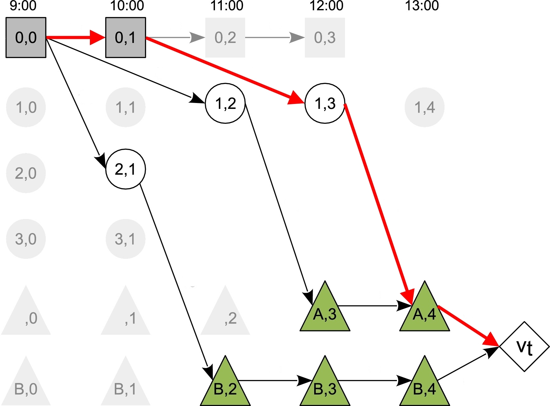
Figure 12: Path $P^{x}$ in the extended time-expanded graph.

The cost of the combination (path,start time), $\text{Cost}(P,t_{0})$, can be calculated by first assigning arc costs $c_{e_{t}}^{\text{sp}}$ to each arc $e_{t}\in\mathcal{A}^{x}$ as follows:

$$c_{e_{t}}^{\text{sp}}=\sum_{t^{\prime}=t}^{|\mathcal{H}|}(c_{e_{t^{\prime}}}-\pi_{e_{t^{\prime}}})\cdot f(t^{\prime}-t)\qquad\forall e_{t}\in\mathcal{A}^{x}\setminus(\mathcal{A}_{w}^{x}\cup\mathcal{A}_{s}^{x})$$ (81)

$$c_{e_{t}}^{\text{sp}}=\bar{c}\cdot(d_{k}-F(|\mathcal{H}|-t))\qquad\forall e_{t}\in\mathcal{A}_{s}^{x}$$ (82)

$$c_{e_{t}}^{\text{sp}}=0\qquad\forall e_{t}\in\mathcal{A}_{w}^{x}$$ (83)

Equation (81) aggregates future costs of arc $e_{t}$, should it be selected for a time-response evacuation plan, while Equation (82) accounts for the cost of evacuees not reaching safety for time-response evacuation plans which end with that arc.

With these arc cost definitions, $\text{Cost}(P,t_{0})$ for a path $P$ and an evacuation start time $t_{0}$ that corresponds to a path $P^{x}$ can be calculated using Equation (84):

$$\text{Cost}(P,t_{0}) =\sum_{e_{t}\in P^{x}}c_{e_{t}}^{\text{sp}}$$ (84)

$$=\bar{c}\cdot(d_{k}-F(|\mathcal{H}|-t))+\sum_{e_{t}\in P^{x}\setminus\mathcal{A}_{s}^{x}}\sum_{t^{\prime}=t}^{|\mathcal{H}|}(c_{e_{t^{\prime}}}-\pi_{e_{t^{\prime}}})\cdot f(t^{\prime}-t)$$ (85)

$$=\bar{c}\cdot\bar{a}_{p}+\sum_{e\in p}\sum_{t\in\mathcal{H}}(c_{e_{t}}-\pi_{e_{t}})\cdot a_{p,e_{t}}$$ (86)

Equations (85) and (86) show that the expansion of (84) will eventually lead to the original equation for $\text{Cost}(P,t_{0})$ in (80).

With this formulation, the goal of the PSP, which is to find a path $P$ and evacuation start time $t_{0}$ combination that minimizes $\text{Cost}(P,t_{0})$, can be accomplished by finding a shortest path from $k_{0}$ to $v_{t}$ in the extended time-expanded graph for each $k\in\mathcal{E}$ and $f\in\mathcal{F}$. This allows a shortest path algorithm such as the Bellman-Ford algorithm to be applied to solve the PSP in polynomial time.

The Contraflow Extension

The CG method can also be extended to produce an evacuation plan that allows for contraflows. It suffices to replace constraints (76) in the RMP with Constraints (87) and (88), and to introduce additional Constraints (89) and (90).

$$\sum_{p\in\omega(e)}a_{p,e_{t}}\cdot x_{p}\leq u_{e_{t}}\qquad\forall e\in\mathcal{A}\setminus\mathcal{A}_{c},\forall t\in\mathcal{H}$$ (87)

$$\sum_{p\in\omega(e)}a_{p,e_{t}}\cdot x_{p}\leq y_{e}\cdot u_{e_{t}}+(1-y_{\bar{e}})\cdot u_{\bar{e}_{t}}\qquad\forall e\in\mathcal{A}_{c},\forall t\in\mathcal{H}$$ (88)

$$y_{e}+y_{\bar{e}}\geq 1\qquad\forall e\in\mathcal{A}_{c}$$ (89)

$$y_{e}\in[0,1]\qquad\forall e\in\mathcal{A}_{c}$$ (90)

Constraints (87) enforce capacity on arcs that may not be used in contraflow, while Constraints (88) do the same for arcs that may. Constraints (89) prevents arcs $e$ and $\bar{e}$ from being used in contraflow simultaneously for road segment $(e,\bar{e})$ with $e\in\hat{\mathcal{A}}_{c},\bar{e}\in\check{\mathcal{A}}_{c}$, and Constraints (90) apply a linear relaxation on variable $y_{e}$. Once the column generation procedure has terminated, variable $y_{e}$ is made binary, the final RMP is solved as a MIP, and the rest of the CG method remains unchanged.

Elementary Paths

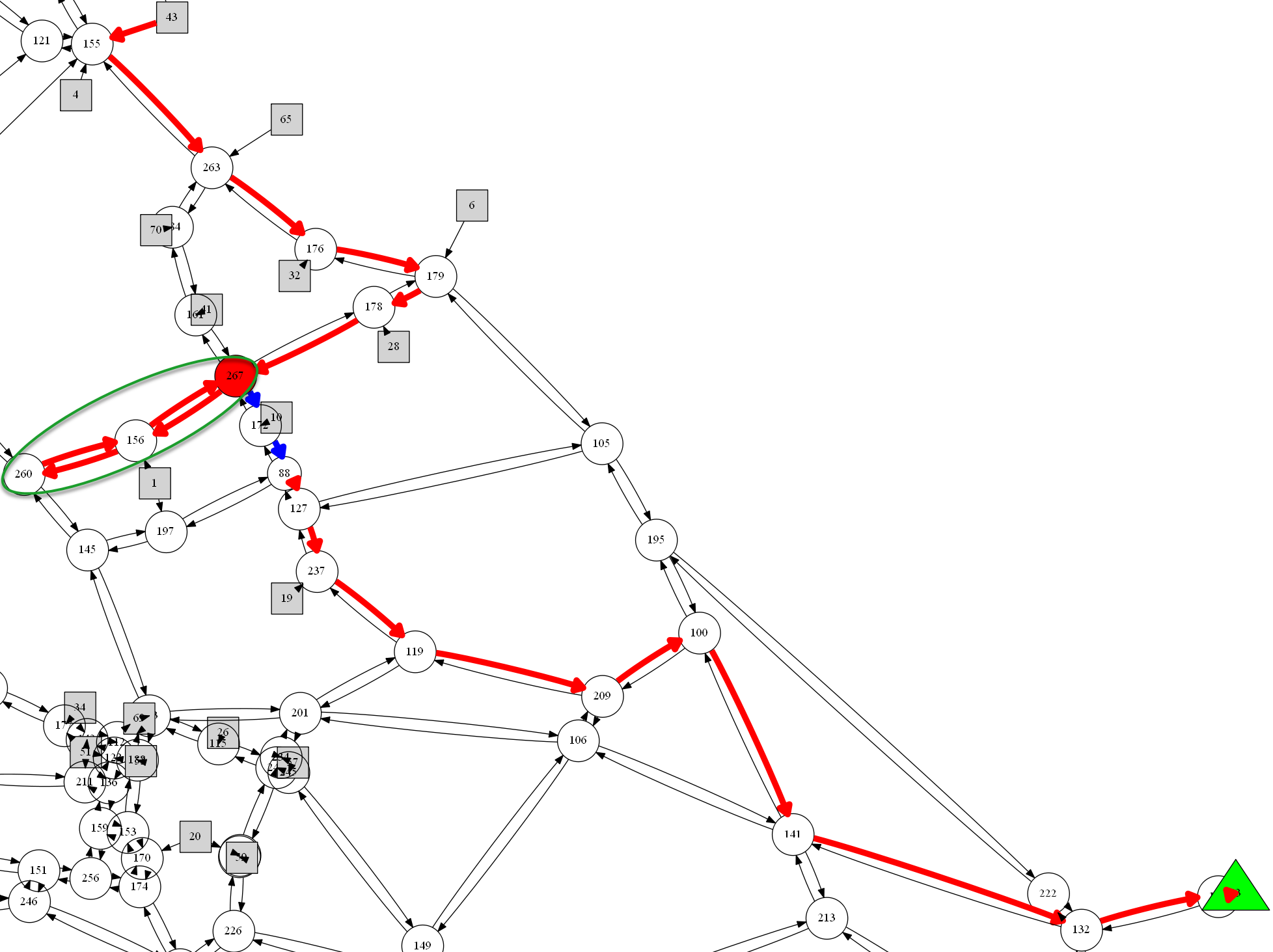
Figure 13: An Example of Non-Elementary Path.

The time-expanded graph $\mathcal{G}^{x}$ is by construction acyclic as its arcs only connect nodes at different time steps. As such, the shortest paths identified in the PSP are also acyclic. However, this fact does not preclude the PSP from generating paths that visit the same transit node in $\mathcal{G}^{x}$ at different time steps, as there are no restrictions enforced in the shortest path algorithms preventing such paths from being generated. While such paths are acyclic in $\mathcal{G}^{x}$, their corresponding counterparts in the static graph $\mathcal{G}$ contain cycles, as they visit the same transit node more than once.

These cyclic paths are called non-elementary (they visit the same node multiple times) and an example of such a non-elementary path is shown in Figure 13. Non-elementary paths in the static graph are undesirable in real evacuations, as they give evacuees the impression that the evacuation plans are sub-optimal and reduce trust in emergency services. However, when the CG algorithm is applied to the real case study, about 44% of the generated evacuation paths are not elementary.

$$\min\sum_{e_{t}\in\mathcal{A}^{x}}c_{e_{t}}^{\text{sp}}\cdot x_{e_{t}}$$ (91)

subject to

$$\sum_{e_{t}\in\delta^{+}(k_{0})}x_{e_{t}}=1$$ (92)

$$\sum_{e_{t}\in\delta^{-}(i)}x_{e_{t}}-\sum_{e_{t}\in\delta^{+}(i)}x_{e_{t}}=0\qquad\forall i\in\mathcal{N}^{x}\setminus\{k_{0},v_{t}\}$$ (93)

$$\sum_{e_{t}\in\delta^{-}(v_{t})}x_{e_{t}}=1$$ (94)

$$\sum_{i_{t}\in\mathrm{\Lambda}(i)}\sum_{e_{t}\in\delta^{+}(i_{t})}x_{e_{t}}\leq 1\qquad\forall i\in\mathcal{T}$$ (95)

$$x_{e_{t}}\in\{0,1\}\qquad\forall e_{t}\in\mathcal{A}^{x}$$ (96)

Figure 14: The Pricing Subproblem With Elementary Paths.

This section outlines the pricing subproblem proposed in [17] that only generates time-response evacuation plans with elementary paths. Let $\mathrm{\Lambda}(i)$ denote the set of time-expanded nodes in $\mathcal{G}^{x}$ for a node $i\in\mathcal{T}$, i.e., $\mathrm{\Lambda}(i)=\{i_{t}\,|\,t\in\mathcal{H}\}$. A path $P^{x}$ in $\mathcal{G}^{x}$ corresponds to an elementary path $P$ in $\mathcal{G}$ if and only if $P^{x}$ visits at most a single node in $\mathrm{\Lambda}(i)$ for each node $i\in\mathcal{T}$. As a result, instead of finding a least-cost path, the revised PSP must find a least-cost path that is also an elementary path in the static graph. Figure 14 depicts the new formulation of the pricing problem. The formulation uses binary decision variable $x_{e_{t}}$ to indicate whether edge $e_{t}$ should be selected as part of the shortest path. Objective function (91) minimizes the total cost of the path. Constraint (92) specifies that exactly one path should emanate from source node $k_{0}$, while constraint (94) ensures the path ends at super sink node $v_{t}$. Constraints (93) enforce path continuity at every node other than the source and super sink. Finally, Constraints (95) guarantee that each transit node is visited by the path at most once throughout the entire time horizon.

This version of the PSP is a shortest path problem with resource constraints [21] which is known to be NP-hard [14]. In this particular formulation, the resources are simply the unit “visited” resources associated with each transit node in $\mathcal{G}^{x}$. The set of all time steps of a particular transit node, $\{i_{t}\,|\,i\in\mathcal{T},\forall t\in\mathcal{H}\}$, is allocated only one unit of this “visited” resource, and the resource is completely consumed if this node were to be visited by a path. For the case study in this paper, this constrained shortest-path problem must be solved repeatedly for a graph with approximately 30000 nodes and 75000 arcs.

While solving formulation (91)-(96) using a MIP solver will result in the desired shortest elementary path, the hybrid strategy proposed in [17] is capable to obtain these paths faster. The hybrid strategy combines the above formulation with a $k$-shortest-path-based algorithm based on the implementation of Jimenez and Marzal’s Recursive Enumeration Algorithm (REA) [22]. This algorithm incrementally generates a $k$^th-shortest path based on information of the $(k-1)$ shortest paths. It can be used to find the shortest elementary path by first generating the shortest path (setting $k=1$). If the path is elementary, the algorithm terminates. Otherwise, the next shortest path is generated by the REA (by incrementing $k$ by 1) and the elementary check is applied on this path. This process is repeated until an elementary path is obtained.

Computational experiments on the case study show that the $k$-shortest-path-based algorithm is extremely fast at finding shortest elementary paths when the required $k$ values are relatively small ($k<10^{5}$). Unfortunately, in some rare instances, the value of $k$ required to obtain an elementary path is extremely large (in the millions), and under these circumstances, solving the MIP formulation produces faster results. Therefore, the hybrid strategy combines both methods by first utilizing the $k$-shortest-path-based algorithm to find shortest elementary paths up to a threshold value for $k$ (in this study, the threshold is set to $10^{5}$). If this $k$-threshold is reached and a elementary path is yet to be found, a MIP formulation is solved. This hybrid strategy exploits the strengths of both methods and is extremely effective at identifying shortest elementary paths quickly in almost all cases.

8 Clearance Time Minimization

Of the four methods presented, only the CG method has a multi-objective function which minimizes total evacuation time in addition to maximizing number of evacuees reaching safety. The BN, BC, and CPG methods only optimize for the latter goal. However, evacuation authorities are also deeply interested in the minimum clearance time, i.e., the smallest amount of time to evacuate an entire region. A precise definition of minimum clearance time, $h^{*}$, is as follows:

$$h^{*}=\min\Bigg{\{}t\in\mathcal{H}\ \bigg{|}\ z(\text{EPP}(\mathcal{G},[0..t]))=\sum_{k\in\mathcal{E}}d_{k}\Bigg{\}}$$ (97)

where $\text{EPP}(G,\mathcal{H})$ denotes the optimal solution obtained from an EPP formulation given static graph $\mathcal{G}$ and time horizon $\mathcal{H}$ as inputs. This section shows how to obtain the minimum clearance time for each method.

Benders Non-convergent and Convergent Methods

The BN and BC methods each consists of an RMP and an SP which generate upper and lower bounds to the objective value. As proposed in [36], a lower bound on the minimum clearance time, $h^{\dagger}$, can first be obtained by performing a binary search over the time horizon using just the RMP. Next, a sequential search using the full BN or BC method can be used to find $h^{*}$, beginning from its lower bound $h^{\dagger}$. This approach seems preferable over a binary search for the second stage as $h^{*}$ is very likely closer to the lower bound $h^{\dagger}$ and hence the second part of the algorithm will converge faster by starting a sequential search from that time. Algorithm 3 summarizes the entire approach.

Algorithm 3 Clearance Time Minimization for BN and BC Methods

1:$h^{\dagger}\leftarrow\min\{t\in\mathcal{H}\,|\,z(\text{RMP}(\mathcal{G},[0..t]))=\sum_{k\in\mathcal{E}}d_{k}\}$

2:$h^{*}\leftarrow\min\{t\in[h^{\dagger}..\mathcal{H}]\,|\,z(\text{EPP}(\mathcal{G},[0..t]))=\sum_{k\in\mathcal{E}}d_{k}\}$

3:return $h^{*}$, evacuation paths from solution of RMP, and evacuation schedule from solution of SP

Conflict-based Path Generation Method

Since the CPG method does not maintain upper and lower bounds to the objective value of the EPP, the clearance time can be performed by a binary search over the time horizon the full CPG method.

Column Generation Method

Even though the CG method’s multi-objective function minimizes total evacuation time, the quantity is not equivalent to clearance time. Clearance time is equivalent to the time at which the last evacuee arrives at its safe node, and this is not the quantity being minimized in the objective function. Minimizing total evacuation time might result in minimal clearance time, but it might also produce suboptimal clearance times as the penalty incurred by late arrival of the last evacuee could possibly be diluted by early arrival costs. Application of a binary search over the time horizon is an option, however this paper did not resort to this approach due to the significant run times of the CG method. Therefore, the minimum clearance time experiments only report the arrival time of the last evacuee produced by the CG method while fully recognizing that it might be suboptimal as the method’s objective function does not explicitly minimize clearance times.

9 The Case Study

This section presents a case study to investigate the effectiveness and run times of the four methods on a real-world evacuation scenario. It also discusses some preliminary observations on various properties of the evacuation algorithms.

The Case Study

The case study is the Hawkesbury-Nepean (HN) region located north-west of Sydney, Australia, which is separated from the Blue Mountains, a catchment area, by the Warragamba dam (See Figure 15. This dam often spills over and, if it breaks, it would create a massive flooding event for West Sydney. The region’s evacuation graph consists of 80 evacuation nodes, 184 transit nodes, and 5 safe nodes. Evacuation node deadlines and road block times for the region were obtained from a hydro-dynamic simulation of a 1-in-100 years flood event. The region has a total of 38,343 vehicles to be evacuated in its base instance; However the results also consider the effect of increasing the population size by linearly scaling the base instance by a factor $x\in[1.0,3.0]$, as West Sidney has sustained significant population growth. Figure 16(a) shows a bird’s-eye view of the entire region, while Figure 16(b) shows its corresponding evacuation graph, with squares, circles, and triangles representing evacuation, transit, and safe nodes respectively. Each instance (or evacuation scenario) is referred to as HN80-Ix from this point forth, where $x$ is the population scaling factor.

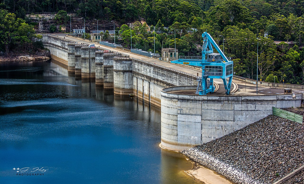
Figure 15: The Warragamba Dam in New South Wales.

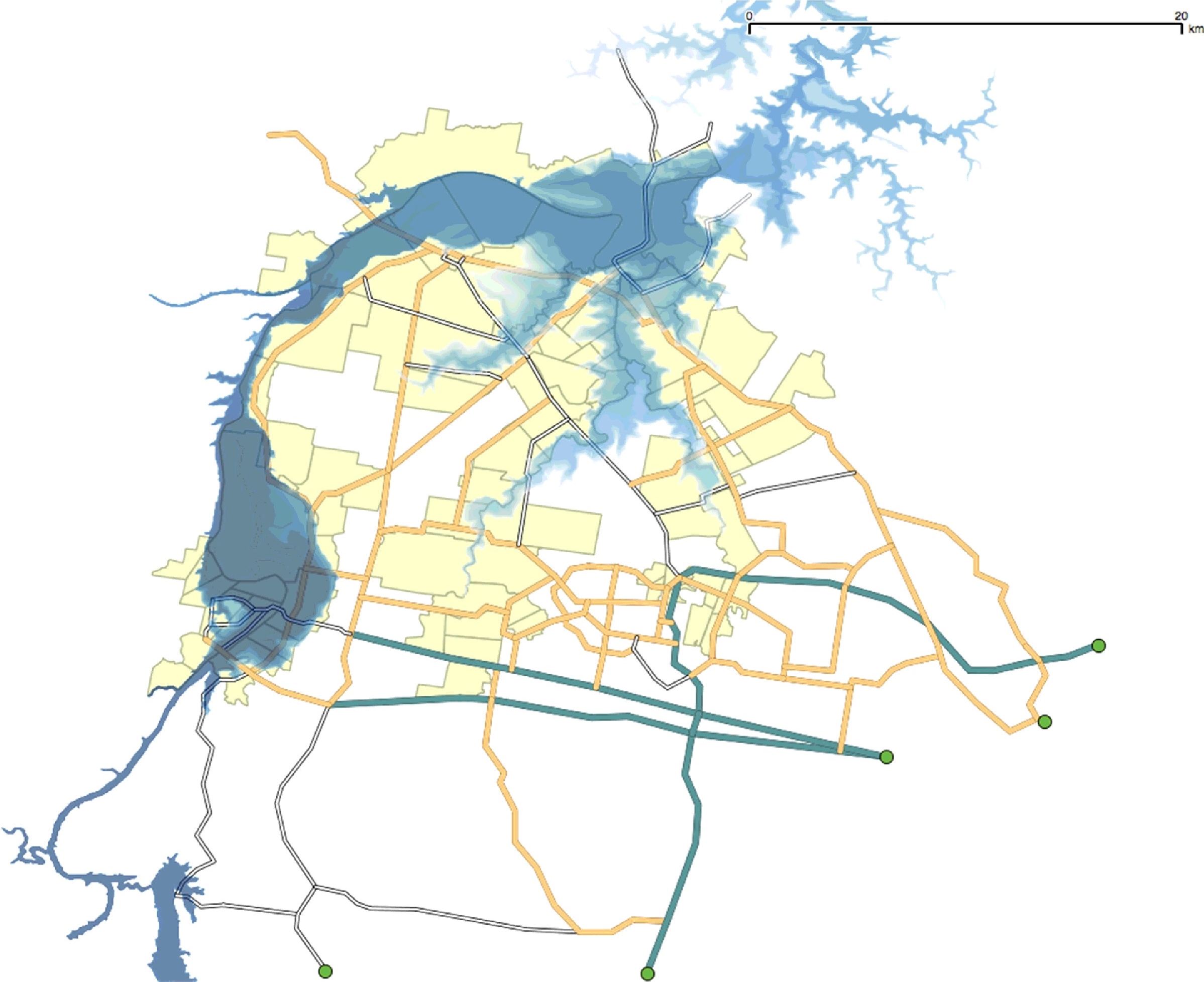
(a) HN map (from [34])

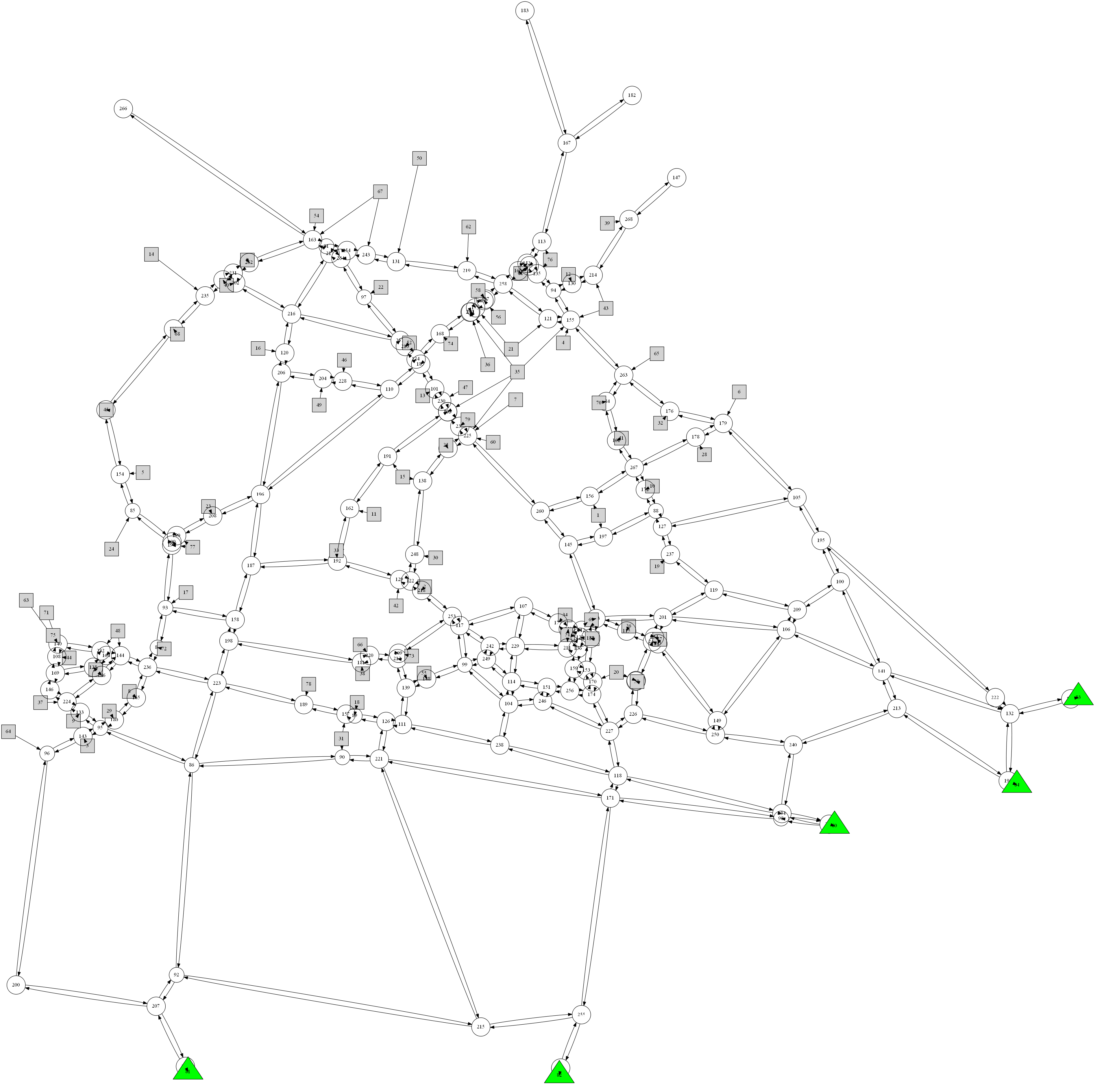
(b) HN evacuation graph

Figure 16: The Map and Evacuation Graph of the Hawkesbury-Nepean Region.

Experimental Settings

The performance of each method is evaluated under two settings: (a) a deadline setting where the maximum number of evacuees reaching safety is determined within a fixed time horizon $\mathcal{H}$ = 10 hours, and (b) a minimum clearance time setting where the smallest amount of time needed to evacuate the entire region is determined. Under both settings, the time horizon is discretized into 5 minute time steps. For the CG method, the set of predefined response curves $\mathcal{F}$ was populated with step response curves with flow rates $\gamma\in\{2,6,10,25,50\}$ evacuees per time step. All methods were implemented in C++, with multi-threaded components being handled using OpenMP, used in conjunction with Gurobi 6.5.2 to solve all mathematical programs. All experiments were conducted on the University of Michigan’s Flux high-performance computing cluster, with each utilizing 8 cores of a 2.5 GHz Intel Xeon E5-2680v3 processor and 64 GB of RAM.

Convergent versus Non-Convergent Paths

Figures 17(a) and 17(b) illustrate examples of generated non-convergent and convergent evacuation paths that do not use contraflow. The paths, whose arcs are represented by red colored arrows, are overlaid on top of the evacuation graph in these figures. It can be seen in Figure 17(b) that convergent paths form a tree with leaves at the evacuation nodes (squares in the graph) and rooted at the safe nodes (triangles in the graph). The non-convergent paths in Figure 17(a) do not share this property; however not being constrained by this property allows more arcs to be utilized for evacuation (at the expense introducing potential delays caused by driver hesitation when multiple paths fork at road intersections).

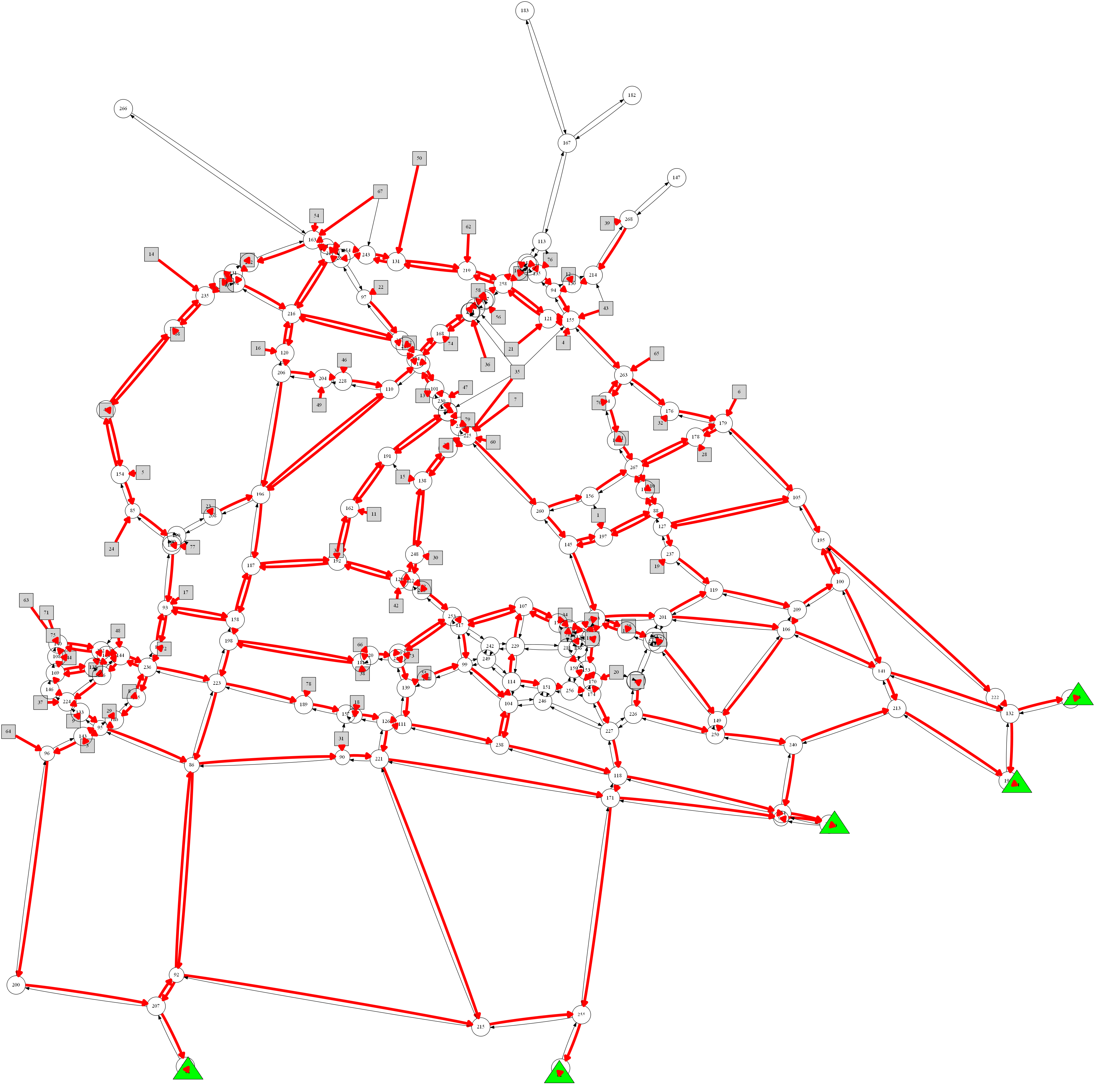
(a) Non-Convergent Evacuation Paths.

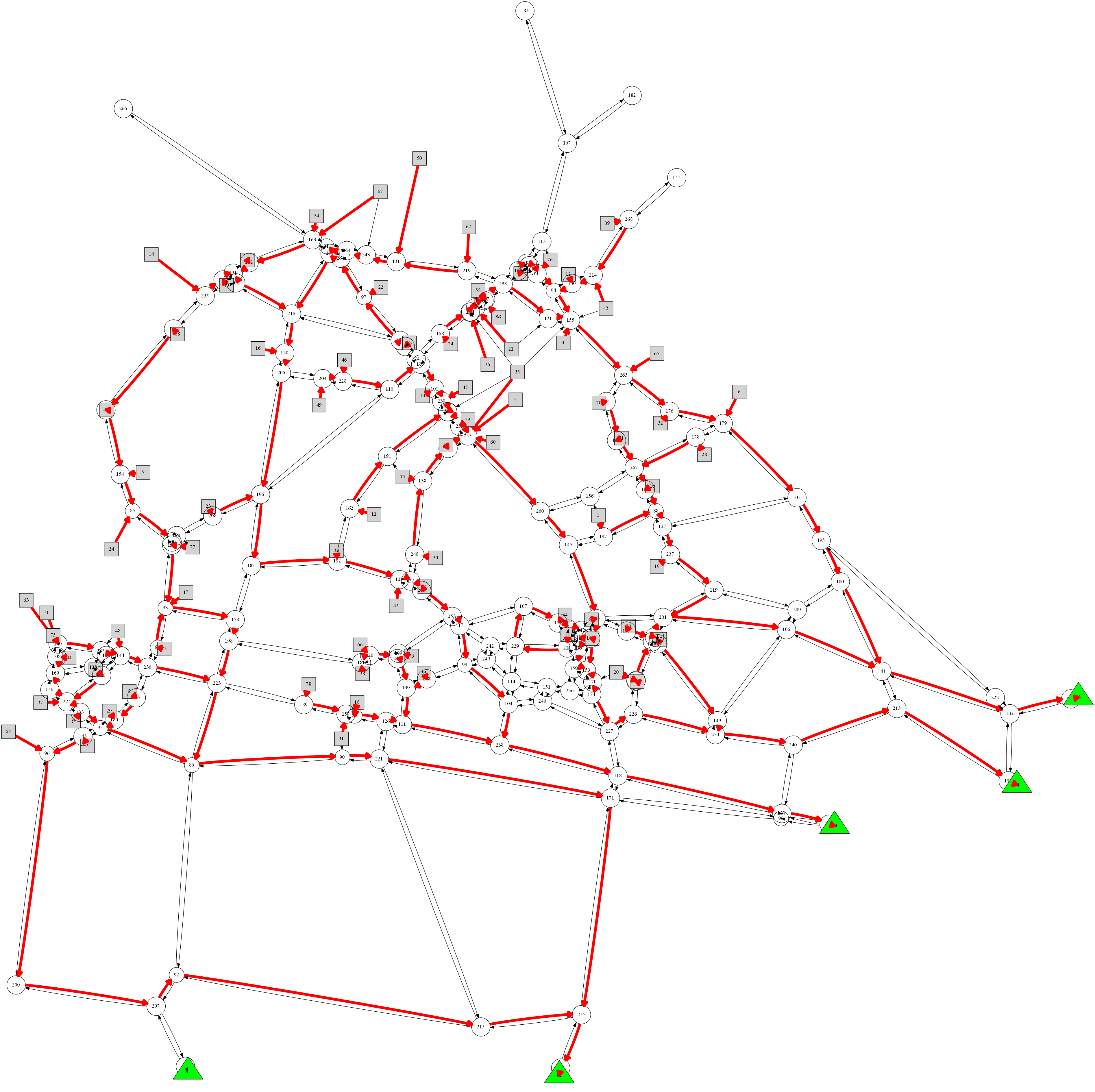
(b) Convergent Evacuation Paths.

Figure 17: Non-Convergent and Convergent Evacuation Paths without Contraflow Generated by the BN and BC Methods.

Preemptive Versus Non-Preemptive Schedules

Figure 18 highlights the difference between preemptive and non-preemptive evacuation schedules generated for an evacuation node with 569 evacuees. The preemptive schedule is characterized by multiple spikes followed by interruptions in evacuee departure rates over time, which may lead to some challenges in the enforcement of the schedule. This is contrasted with the non-preemptive schedule which uses a step response curve with a flow rate of 25 evacuees every 5 minutes. Evacuation is started at the 85^th minute, and a constant departure rate is maintained until the node has been completely evacuated, making the schedule arguably easier to enforce compared to the preemptive one.

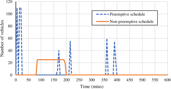
Figure 18: Preemptive and Non-Preemptive Evacuation Schedules for an Evacuation Node with 569 Evacuees (Generated by the BN and CG Methods Respectively).

Convergence of the Benders Decomposition

Figures 19(a) and 19(b) reveal how the upper and lower bounds of the BN and BC methods converge over time for a particular experiment in the deadline setting. For this instance, the BC method converged in less than 140 iterations, while the BN method did not, even after 360 iterations, at which point the algorithm was terminated as it exceeded a set time limit (time limits for each method are elaborated further in Section 10). Nevertheless, it can be seen that final optimality gap is very small ($\approx 0.2\%$) and this gap was attained in less than 40 iterations.

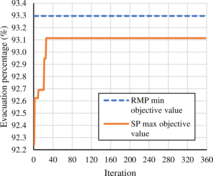
(a) Convergence of the BN Method

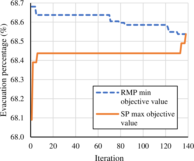
(b) Convergence of BC Method

Figure 19: Convergence characteristics of the BN and BC methods under the deadline setting for the HN80-I3.0 instance.

Elementary and Non-Elementary Paths

Table 1 compares results of the column generation phase of the CG method without and with the elementary path restriction. The key takeaway is that the two formulations produce the same optimal values. Minor differences in the last two instances may be due to the column generation phase being terminated before convergence as a CPU time limit of 5760 minutes was reached (CPU time limits applied to all experiments are detailed further in Section 10.1). Restricting attention to elementary paths increases the CPU times, which is not surprising, since finding shortest paths subject to resource constraints is an NP-hard problem: Even though the hybrid strategy employed for finding elementary paths is highly effective, it still cannot compete with the polynomial time Bellman-Ford algorithm used in the original formulation. Nevertheless, it is interesting to observe that the CPU time advantage of the original formulation diminishes as the population size increases. Another intriguing observation is that CG with elementary paths reaches optimality in fewer iterations and it has fewer columns in its final RMP in almost all instances.

Instance	Original Shortest Path PSP				New Elementary Shortest Path PSP
	Iter #	Column #	CPU Time (mins)	Optimal Obj Val	Iter #	Column #	CPU Time (mins)	Optimal Obj Val
HN80-I1.0	79	12251	39	8816	79	11678	124	8816
HN80-I1.1	104	15072	136	10405	95	13853	218	10405
HN80-I1.2	229	22571	799	12116	190	19543	834	12116
HN80-I1.4	152	20184	690	15935	108	17048	404	15935
HN80-I1.7	178	21871	1312	22635	120	19883	2760	22635
HN80-I2.0	197	31418	5760	30490	145	25051	5760	30490
HN80-I2.5	121	22806	5760	46189	129	23513	5760	46188
HN80-I3.0	132	31726	5760	$1.960\times 10^{9}$	87	21233	5760	$1.961\times 10^{9}$

Table 1: Results of column generation phase of CG method using original shortest path and new elementary shortest path PSP formulations (when no contraflow is allowed).

Convergence of the Column Generation

Figure 20 demonstrates how the objective value of the RMP of the CG method evolves over time during its column-generation phase. It also shows the evolution of the objective value of the best incumbent solution found for the RMP when it is solved as an IP in its last iteration, together with the progression of its optimality gap over time. It can be seen that there is a steep decline in the objective value of the restricted master problem within the first 100 seconds, after which the value slowly approaches a minimum. The same trend is observed when the restricted master problem is solved as a MIP, with the optimality gap of the best incumbent solution settling to a value of $\approx 13.5\%$ when the algorithm reached its time limit.

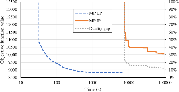
Figure 20: Evolution of the solution quality of the CG method over time for the HN80-I1.0 instance.

10 Macroscopic Evaluation

This section provides a summary of the results obtained from all four methods under the deadline and minimum clearance time settings, together with the specific conditions under which each method is applied.

10.1 The Deadline Setting

Under the deadline setting, each method maximizes the number of evacuees reaching safety for the HN80-Ix instances (with x $\in[1.0,3.0]$) within a fixed time horizon $\mathcal{H}$ = 10 hours.

The BN Method

The results of the BN method are summarized in Tables 2 and 3 without and with contraflow respectively. As shown in Algorithm 1, BN first searches for the tightest time horizon $t^{*}$ that can preserve the optimal solution of the RMP, $z(\text{RMP}(\mathcal{G},\mathcal{H}))$. The tables show the CPU time taken for this first phase in column “$t^{*}$ CPU Time”. Each RMP instance in this procedure is given a CPU time limit of 10 minutes. The tables also show the total number of iterations required to complete the entire method as well as the corresponding total CPU time taken. The complete method is allocated a CPU time limit of 24 hours. Finally, the tables show the minimum objective value of the RMP $z_{\text{RMP}}$ and the maximum objective value of the SP, $z_{\text{SP,max}}$ at termination in terms of evacuation percentage, as well as the optimality gap, i.e., the percentage difference between the upper and lower bounds of the solution given by $\frac{z_{\text{RMP}}-z_{\text{SP,max}}}{z_{\text{SP,max}}}$.

There are three key observations from Tables 2 and 3: (a) Without contraflows, the method converges to an evacuation percentage of 100% for all instances except for HN80-I3.0, for which the method produces a 93.1% evacuation percentage. This was also the only instance where the method did not converge within the allocated CPU time limit; however the final optimality gap of 0.20% assures that the obtained solution is very close to being optimal. (b) The method converges after only 1 iteration for all instances except HN80-I2.5 and HN80-I3.0 without contraflow. For instances that took 1 iteration, the bulk of the CPU time is spent on the search for $t^{*}$. (c) When using contraflows, the method converges faster on all instances: The increased network capacity provided by contraflows makes the evacuation instances easier to solve.

Instance	Iter #	$\boldsymbol{t^{*}}$ CPU Time (mins)	Total CPU Time (mins)	$\boldsymbol{z_{\text{RMP}}}$ (%)	$\boldsymbol{z_{\text{SP,max}}}$ (%)	Optimality Gap (%)
HN80-I1.0	1	131	135	100.0	100.0	0.00
HN80-I1.1	1	111	117	100.0	100.0	0.00
HN80-I1.2	1	104	110	100.0	100.0	0.00
HN80-I1.4	1	92	96	100.0	100.0	0.00
HN80-I1.7	1	103	110	100.0	100.0	0.00
HN80-I2.0	1	79	84	100.0	100.0	0.00
HN80-I2.5	4	38	98	100.0	100.0	0.00
HN80-I3.0	358	5	1449	93.3	93.1	0.20

Table 2: Results of the BN method under the deadline setting without contraflow.

Instance	Iter #	$\boldsymbol{t^{*}}$ CPU Time (mins)	Total CPU Time (mins)	$\boldsymbol{z_{\text{RMP}}}$ (%)	$\boldsymbol{z_{\text{SP,max}}}$ (%)	Optimality Gap (%)
HN80-I1.0	1	43	47	100.0	100.0	0.00
HN80-I1.1	1	43	45	100.0	100.0	0.00
HN80-I1.2	1	41	43	100.0	100.0	0.00
HN80-I1.4	1	48	50	100.0	100.0	0.00
HN80-I1.7	1	42	45	100.0	100.0	0.00
HN80-I2.0	1	42	45	100.0	100.0	0.00
HN80-I2.5	1	36	39	100.0	100.0	0.00
HN80-I3.0	1	35	37	100.0	100.0	0.00

Table 3: Results of the BN method under the deadline setting with contraflow.

The BC Method

Tables 4 and 5 show results of the BC method under the deadline setting without and with contraflow respectively. The tables are similar to Tables 2 and 3 because of the similarities between the BN and BC methods. The CPU time limits allocated for the BC method are different however: Each RMP instance in the search for $t^{*}$ is given a limit of 10 minutes, whereas the entire method is allocated only 2 hours of CPU time due its faster convergence.

The key observations from these two tables are as follows: (a) The method evacuates everyone for all instances when contraflow is allowed, and for instances HN80-Ix with x $\in[1.0,1.7]$ when contraflow is not allowed. However, unlike the BN method, this method converges to optimal solutions for all instances as evidenced by their 0% optimality gaps. (b) For instances in which a 100% evacuation rate is achieved, the method converges in just 1 iteration, and the bulk of the CPU time in these instances is spent searching for $t^{*}$. (c) Except for instance HN80-I1.4, the method converges faster when contraflow is allowed. As mentioned earlier, the BC method is extremely effective in finding high-quality evacuations quickly.

Instance	Iter #	$\boldsymbol{t^{*}}$ CPU Time (mins)	Total CPU Time (mins)	$\boldsymbol{z_{\text{RMP}}}$ (%)	$\boldsymbol{z_{\text{SP,max}}}$ (%)	Optimality Gap (%)
HN80-I1.0	1	0.35	0.51	100.0	100.0	0.00
HN80-I1.1	1	10.19	10.28	100.0	100.0	0.00
HN80-I1.2	1	10.15	10.24	100.0	100.0	0.00
HN80-I1.4	1	1.13	1.21	100.0	100.0	0.00
HN80-I1.7	1	10.21	10.32	100.0	100.0	0.00
HN80-I2.0	14	0.09	1.80	96.9	96.9	0.00
HN80-I2.5	22	0.28	3.43	81.4	81.4	0.00
HN80-I3.0	138	0.01	16.22	68.5	68.5	0.00

Table 4: Results of the BC method under the deadline setting without contraflow.

Instance	Iter #	$\boldsymbol{t^{*}}$ CPU Time (mins)	Total CPU Time (mins)	$\boldsymbol{z_{\text{RMP}}}$ (%)	$\boldsymbol{z_{\text{SP,max}}}$ (%)	Optimality Gap (%)
HN80-I1.0	1	0.19	0.27	100.0	100.0	0.00
HN80-I1.1	1	0.22	0.30	100.0	100.0	0.00
HN80-I1.2	1	0.28	0.37	100.0	100.0	0.00
HN80-I1.4	1	2.31	2.42	100.0	100.0	0.00
HN80-I1.7	1	0.50	0.60	100.0	100.0	0.00
HN80-I2.0	1	0.61	0.70	100.0	100.0	0.00
HN80-I2.5	1	0.38	0.48	100.0	100.0	0.00
HN80-I3.0	1	0.20	0.30	100.0	100.0	0.00

Table 5: Results of the BC method under the deadline setting with contraflow.

The CPG Method

Results for the CPG method are outlined in Tables 6 and 7 respectively. The tables show the number of iterations, the CPU time, and the evacuation percentage. As mentioned in Section 6, the CPG algorithm is allowed a maximum of 10 iterations, after which it was terminated even if it still had critical nodes which are not completely evacuated. Additionally, the RMP and SP are each allocated a CPU time limit of 1 hour.

The tables show that a 100% evacuation rate is achieved in all instances but HN80-I2.5 and HN80-I3.0 without contraflow. These two instances were terminated by the iteration limit. The results also show relatively short CPU times of less than a minute for instances HN80-Ix with x $\in[1.0,2.0]$, and a spike in CPU time for instance HN80-I3.0 both with and without contraflow. This is possibly caused by the increase in difficulty of solving these instances. The positive correlation between the number of iterations required and the value of x for the instances provides further evidence that the heuristic requires more iterations to evacuate more evacuees. Similar to the BN and BC methods, the CPU times for each instance are smaller when contraflow is allowed. On almost all instances, the CPG method is very effective as well.

Instance	Iter #	CPU Time (mins)	Evacuation Percentage (%)
HN80-I1.0	2	0.05	100.0
HN80-I1.1	3	0.07	100.0
HN80-I1.2	3	0.08	100.0
HN80-I1.4	3	0.10	100.0
HN80-I1.7	3	0.15	100.0
HN80-I2.0	4	0.69	100.0
HN80-I2.5	10	11.04	96.7
HN80-I3.0	10	96.48	86.3

Table 6: Results of deadline setting CPG method without contraflow.

Instance	Iter #	CPU Time (mins)	Evacuation Percentage (%)
HN80-I1.0	1	0.04	100.0
HN80-I1.1	1	0.03	100.0
HN80-I1.2	2	0.04	100.0
HN80-I1.4	2	0.05	100.0
HN80-I1.7	2	0.06	100.0
HN80-I2.0	3	0.15	100.0
HN80-I2.5	4	2.44	100.0
HN80-I3.0	4	21.23	100.0

Table 7: Results of the CPG method under the deadline setting with contraflow.

The CG Method

The results of the CG method without and with contraflow are summarized in Tables 8 and 9 respectively. They show the number of iterations and the CPU time taken by the column generation phase to converge, the total number of columns generated by the phase, the total CPU time taken by the entire CG method, the optimality gap of the final integer solution of the RMP, calculated using formula $\frac{z_{\text{RMP,MIP}}-z_{\text{RMP,LP}}}{z_{\text{RMP,MIP}}}$ where $z_{\text{RMP,LP}}$ an d $z_{\text{RMP,MIP}}$ are the final objective values of the column generation and the MIP respectively, and the evacuation percentage achieved by the method. A couple of CPU time limits are applied to the method: 96 hours for the column generation phase and 24 hours for the final MIP.

The tables show that the final MIP reaches its 24 hour time limit in all instances. The column-generation phase also reaches its 96 hour time limit in the most challenging instances, HN80-Ix with x $\in[2.0,3.0]$ without contraflow and HN80-I3.0 with contraflow. A 100% evacuation rate is achieved in instances HN80-Ix with x $\in[1.0,1.4]$ without contraflow and with x $\in[1.0,2.0]$ with contraflow. Correspondingly, the optimality gaps of these instances are relatively low, being $<20\%$ when contraflow is not allowed and $<10\%$ when it is allowed. This indicates that the quality of the solutions obtained for these instances are relatively high. The large optimality gap of the other instances can be explained by the large penalty incurred in their objective values because not everyone is evacuated safely in the final integer solutions. A steady increase in CPU times is also observed as the population scaling factor x increases. For the same instance, the CPU times are smaller when contraflow is allowed, and so are the optimality gaps when 100% evacuation is achieved.

Instance	Iter #	Column #	Column Generation CPU Time (mins)	Total CPU Time (mins)	Optimality Gap (%)	Evacuation Percentage (%)
HN80-I1.0	75	11626	153	1593	13.5	100.0
HN80-I1.1	88	13463	261	1701	14.9	100.0
HN80-I1.2	191	18020	792	2232	15.0	100.0
HN80-I1.4	116	17412	681	2121	16.9	100.0
HN80-I1.7	119	19415	1275	2715	100.0	96.1
HN80-I2.0	163	25883	5760	7200	100.0	92.5
HN80-I2.5	126	23185	5760	7200	100.0	89.7
HN80-I3.0	95	23146	5760	7200	63.0	81.1

Table 8: Results of the CG method under the deadline setting without contraflow.

Instance	Iter #	Column #	Column Generation CPU Time (mins)	Total CPU Time (mins)	Optimality Gap (%)	Evacuation Percentage (%)
HN80-I1.0	60	3757	25	1465	4.2	100.0
HN80-I1.1	69	4636	55	1495	4.5	100.0
HN80-I1.2	105	5398	137	1577	5.1	100.0
HN80-I1.4	152	8015	304	1744	5.0	100.0
HN80-I1.7	226	11880	829	2269	7.1	100.0
HN80-I2.0	310	14971	1899	3339	9.9	100.0
HN80-I2.5	453	21474	5741	7181	99.9	99.7
HN80-I3.0	201	17094	5760	7200	99.9	99.8

Table 9: Results of the CG method under the deadline setting with contraflow.

Comparison of the Evacuation Rates

Figures 21 and 22 compare the evacuation percentages achieved by all four methods. Figure 22 compares the performance of each method when contraflow is allowed, and it can be seen that all methods achieve 100% evacuation for all instances, except for the CG method which achieves 99.7% and 99.8% evacuation for HN80-I2.5 and HN80-I3.0 respectively. The performance comparison of each method without contraflow is shown in Figure 21 which paints a slightly different picture. All methods achieve 100% evacuation only up to instance HN80-I1.4. For instances with larger population scaling factors, the percentage evacuation starts to drop off significantly for some methods and slightly for others. A common trend prevalent in these instances (HN80-Ix with x $\in[1.7,3.0]$) is that the BN method consistently produces the highest evacuation percentage, followed by CPG. Although both methods generate evacuation plans with the same characteristics, their performance disparity could be attributed to the heuristic nature of CPG: The BN method, although not strictly optimal, returns optimal results when the integrality constraints on flows is relaxed. The lower evacuation rate of the BC and CG methods can be explained by the additional constraints imposed on their respective evacuation plans: The BC method produces convergent paths and the CG method generates non-preemptive evacuation schedules. These constraints limit their ability of matching the performance of the BN and CPG methods in a macroscopic analysis. Indeed, the benefits of these methods cannot be captured in a macroscopic analysis, as they concern human behavior and the realities of enforcing evacuation plans. Note also that the CG method is unique in that the evacuation rates of its plans are limited to the set of predefined flow rates $\gamma$ that was specified in Section 9, whereas the same limitation does not apply to the other methods. The method’s performance is dependent on these preset $\gamma$ values, and that its performance would change given different sets of $\gamma$ values.

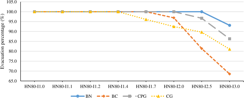
Figure 21: Evacuation percentage under deadline setting without contraflow summary.

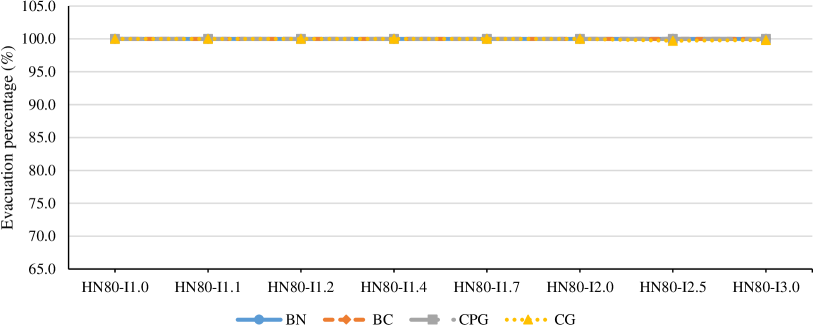
Figure 22: Evacuation percentage under deadline setting with contraflow summary.

Comparison of the CPU Times

Tables 10 and 11 compile the total CPU times of all four methods without and with contraflow respectively. The tables also show average CPU times for each method across all instances with their associated standard errors representing uncertainty. The standard errors are relatively large for most methods due to the spread in CPU times across the various instances. Nevertheless, a quantitative comparison can still be made. Regardless of whether contraflow is allowed or not, the BC and CPG methods consistently consume the smallest amount of CPU time, followed by the BN method, and finally the CG method. On top of being the most expensive method, the CG method reaches its CPU time limit in a few of the more challenging instances. The difference in run times across the different methods is not surprising due to the different algorithms employed as well as the varying constraints imposed on their evacuation plans.

Instance	Total CPU Time (mins)
	BN	BC	CPG	CG
HN80-I1.0	135	0.51	0.05	1593
HN80-I1.1	117	10.28	0.07	1701
HN80-I1.2	110	10.24	0.08	2232
HN80-I1.4	96	1.21	0.10	2121
HN80-I1.7	110	10.32	0.15	2715
HN80-I2.0	84	1.80	0.69	7200
HN80-I2.5	98	3.43	11.04	7200
HN80-I3.0	1449	16.22	96.48	7200
Average	275 $\pm$ 168	6.75 $\pm$ 2.04	13.58 $\pm$ 11.92	3995 $\pm$ 946

Table 10: CPU times of all methods under deadline setting without contraflow.

Instance	Total CPU Time (mins)
	BN	BC	CPG	CG
HN80-I1.0	47	0.27	0.04	1465
HN80-I1.1	45	0.30	0.03	1495
HN80-I1.2	43	0.37	0.04	1577
HN80-I1.4	50	2.42	0.05	1744
HN80-I1.7	45	0.60	0.06	2269
HN80-I2.0	45	0.70	0.15	3339
HN80-I2.5	39	0.48	2.44	7181
HN80-I3.0	37	0.30	21.23	7200
Average	44 $\pm$ 2	0.68 $\pm$ 0.25	3.00 $\pm$ 2.62	3284 $\pm$ 880

Table 11: CPU times of all methods under deadline setting with contraflow.

The disparity in CPU times between the BN and BC methods deserves special attention as their algorithms share a lot of similarities, both utilizing Benders decomposition. This discrepancy is explained by the sizes of the RMP and SP of both methods, which are summarized in Table 12. Although the BC method solves three problems (the RMP, SP, and DMWP) during each iteration and the BM method solves only two, the number of variables and constraints in the latter is significantly larger, leading to correspondingly larger CPU times. Moreover the nature of the subproblem is fundamentally different: The Benders subproblems of the BC method are maximum flows, whereas those of the BN method are multi-commodity flow problems, where evacuees from an evacuation node can be seen as a single commodity.

		BC Method	BN Method
Restricted Master Problem	Constraint #	$|\mathcal{T}|+|\mathcal{E}\cup\mathcal{T}|+|\mathcal{A}|+|\mathcal{E}|+|\mathcal{C}|+1$	$|\mathcal{E}|^{2}+2|\mathcal{T}||\mathcal{E}|+|\mathcal{E}|+|\mathcal{A}||\mathcal{E}|+|\mathcal{A}|+|\mathcal{A}_{c}|+|\mathcal{C}|+1$
	Variable #	$2|\mathcal{A}|+1$	$2|\mathcal{A}||\mathcal{E}|+|\mathcal{A}_{c}|+1$
Subproblem	Constraint #	$|\mathcal{T}||\mathcal{H}|+|\mathcal{A}||\mathcal{H}|+|\mathcal{E}|$	$|\mathcal{T}||\mathcal{H}||\mathcal{E}|+|\mathcal{E}|+|\mathcal{A}||\mathcal{H}||\mathcal{E}|+|\mathcal{A}||\mathcal{H}|$
	Variable #	$|\mathcal{A}||\mathcal{H}|$	$|\mathcal{A}||\mathcal{H}||\mathcal{E}|$
Dual of Magnanti-Wong Problem	Constraint #	$|\mathcal{T}||\mathcal{H}|+|\mathcal{A}||\mathcal{H}|+|\mathcal{E}|$	-
	Variable #	$|\mathcal{A}||\mathcal{H}|+1$	-

Table 12: Number of constraints and variables in the problems of the BC and BN methods.

10.2 The Minimum Clearance Time Setting

In the minimum clearance time experiments, each method finds the smallest amount of time needed to evacuate the entire region, i.e., to achieve 100% evacuation. A precise definition of minimum clearance time $h^{*}$ is given in Equation (97).

As explained in Section 8, the CG method’s multi-objective function simultaneously minimizes the overall evacuation time and maximizes the evacuation percentage. As such, $h^{*}$ can be determined from its deadline setting results for instances where 100% evacuation is achieved by identifying the time at which the last evacuee reaches its safe node. For the BN and BC methods, the approach outlined in Section 8 is applied to find $h^{*}$. As summarized in Algorithm 3, a binary search procedure is first applied to find a lower bound $h^{\dagger}$ to the minimum clearance time. A sequential search procedure is then applied to find $h^{*}$. For both methods, a CPU time limit of 10 minutes is applied when solving each RMP instance in the binary search procedure. However, in the subsequent sequential search, a CPU time limit of 10 hours is used for each search step of the BN method, while a time limit of 2 hours is used for that of the BC method. The different time limits are selected to cater for the correspondingly different convergence times of each method. The approach outlined in Section 8 is used to find $h^{*}$ for the CPG method. Under the minimum clearance time setting, the method’s RMP and SP are each allocated only 2 minutes of CPU time.

Instance	BN		BC		CPG		CG
	CPU Time (mins)	Min Clear Time (mins)	CPU Time (mins)	Min Clear Time (mins)	CPU Time (mins)	Min Clear Time (mins)	CPU Time (mins)	Min Clear Time (mins)
HN80-I1.0	814	260	11	335	29	280	1593	455
HN80-I1.1	1936	290	12	365	27	315	1701	555
HN80-I1.2	650	300	10	395	38	330	2232	570
HN80-I1.4	1440	350	13	450	35	380	2121	600
HN80-I1.7	690	405	10	535	55	445	-	-
HN80-I2.0	705	470	10	630	41	520	-	-
HN80-I2.5	1374	575	2	770	94	625	-	-
HN80-I3.0	1128	675	16	925	67	815	-	-

Table 13: Minimum clearance times of all methods without contraflow.

Instance	BN		BC		CPG		CG
	CPU Time (mins)	Min Clear Time (mins)	CPU Time (mins)	Min Clear Time (mins)	CPU Time (mins)	Min Clear Time (mins)	CPU Time (mins)	Min Clear Time (mins)
HN80-I1.0	500	195	26	225	46	200	1465	235
HN80-I1.1	624	205	27	240	56	210	1495	255
HN80-I1.2	713	225	47	260	57	235	1577	285
HN80-I1.4	49	250	3	285	79	260	1744	320
HN80-I1.7	207	290	1	335	56	320	2269	575
HN80-I2.0	49	335	10	390	63	385	3339	535
HN80-I2.5	52	405	10	475	99	440	-	-
HN80-I3.0	59	475	0	560	106	500	-	-

Table 14: Minimum clearance times of all methods with contraflow.

The total CPU times and the value of $h^{*}$ for each method are presented in Tables 13 and 14 for cases without and with contraflow respectively. For the CG method, results are only shown for instances where the method achieved 100% evacuation under the deadline setting. Figures 23 and 24 compare each method without and with contraflow respectively. As expected, the clearance times increase as the population grows and contraflows help reducing them. Across all instances, the BN method consistently produces the smallest clearance time, followed by CPG, BC, and CG. A slight anomaly is observed in the results of the CG method for instances HN80-I1.7 and HN80-I2.0 when contraflow is allowed, where the clearance time is smaller for the latter instance. This result is likely caused by the early termination of the RMP’s last iteration, in which it reached its 24 hours CPU time limit.

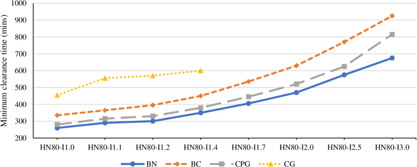
Figure 23: Minimum clearance time without contraflow summary.

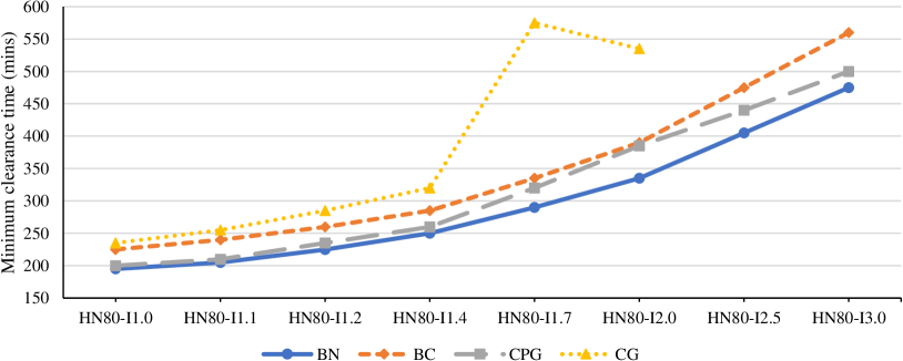
Figure 24: Minimum clearance time with contraflow summary.

Finally, Table 15 shows the average CPU times consumed by each method under the minimum clearance time setting. Whether contraflow is allowed or not, the BC method consistently consumes the least amount of CPU time, followed by CPG, BN, and CG.

Method	Average CPU Time (mins)
	Without Contraflow	With Contraflow
BN	1092 $\pm$ 164	282 $\pm$ 101
BC	11 $\pm$ 1	16 $\pm$ 6
CPG	48 $\pm$ 8	70 $\pm$ 8
CG	1912 $\pm$ 156	1981 $\pm$ 297

Table 15: Average CPU times of all methods under minimum clearance time setting.

11 Microscopic Evaluation

The four evacuation methods presented in this paper are macroscopic and do not capture individual evacuee behaviors, movements, and interactions, as well as vehicle dynamics such as acceleration and deceleration, lane changing, and collision avoidance which are all reflective of what would actually happen in a real world evacuation scenario. These factors could introduce unanticipated delays or induce congestion, both of which would negatively affect the performance of an evacuation plan. Unfortunately, these factors are not captured in the macroscopic evaluation.

This section presents a microscopic evaluation of the four evacuation algorithms. Each evacuation plans was simulated, using a road traffic simulation package SUMO (Simulation of Urban Mobility) [23]. SUMO is a full-featured, open-source, microscopic traffic flow simulation suite developed primarily by researchers of the Institute of Transportation Systems at the German Aerospace Center. Its traffic simulator realistically models the traversal behavior of each vehicle in a road network by computing each vehicle’s instantaneous speed according to the speed limit, a safe distance to be maintained from a leading vehicle, and the leading vehicle’s speed according to a car-following model described in [24] and a lane changing model described in [10]. This simulator not only allows for ascertaining and evaluating the robustness of the evacuation plans generated in terms of how they would actually perform in a real world evacuation scenario; it can also reveal the benefits of convergent and non-preemptive plans.

The simulations utilize actual road network information of the HN region, including speed limits, lane counts, and GPS coordinates of each node to construct the road network for SUMO. They also define the demand by specifying, for each vehicle, an evacuation path and a departure time derived from plans generated in the deadline and minimum clearance time experiments.

11.1 The Deadline Setting

Table 16 shows the evacuation percentages obtained from simulating the evacuation plans generated by the deadline setting experiments. Figures 25 and 26 present the same information in graphical form for settings without and with contraflow respectively. To get a better perspective on the results shown in these figures, they should be compared with their counterparts from the deadline experiments, Figures 21 and 22, which show corresponding evacuation percentages produced by the four algorithms. When contraflows are not allowed, the evacuation percentages start to decrease sooner as the population scaling factor increases. More importantly, the clear performance advantage of the BN and CPG methods are not preserved in these simulations: In some instances, they are outperformed by the other two methods while, for some other instances, they could barely outperform the CG method. When contraflows are allowed, the methods are no longer able to achieve a 100% evacuation rate. In fact, the CPG method cannot achieve a 100% evacuation on any instance, while the evacuation percentage of other methods start decreasing after instance HN80-I2.0., with the BN method having the steepest drop.

Instance	Evacuation Percentage (%)
	Without Contraflow				With Contraflow
	BN	BC	CPG	CG	BN	BC	CPG	CG
HN80-I1.0	100.0	100.0	100.0	100.0	100.0	100.0	97.6	100.0
HN80-I1.1	100.0	100.0	98.8	100.0	100.0	100.0	95.0	100.0
HN80-I1.2	100.0	100.0	97.6	100.0	100.0	100.0	94.3	100.0
HN80-I1.4	100.0	100.0	95.1	100.0	100.0	100.0	98.3	100.0
HN80-I1.7	91.1	95.6	94.9	96.1	100.0	100.0	94.8	100.0
HN80-I2.0	94.4	85.2	90.6	92.2	100.0	100.0	94.2	100.0
¡ HN80-I2.5	80.2	70.9	84.8	80.2	94.3	100.0	89.7	98.9
HN80-I3.0	70.4	61.4	67.7	67.4	70.2	92.3	77.7	91.3

Table 16: Evacuation percentages obtained from SUMO simulations of deadline setting evacuation plans.

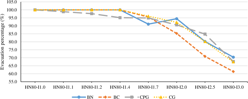
Figure 25: Evacuation percentages obtained from SUMO simulations of deadline setting evacuation plans without contraflow.

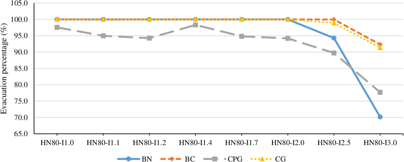
Figure 26: Evacuation percentages obtained from SUMO simulations of deadline setting evacuation plans with contraflow.

In order to obtain a better understanding of how closely the simulated results match those of deadline experiments, it is interesting to normalize the evacuation percentage obtained from the simulations relative to those from the deadline settings. More precisely, the normalized evacuation percentage is calculated as follows:

$$\text{Normalized evacuation percentage}=\frac{\text{microscopic evacuation percentage}}{\text{macroscopic evacuation percentage}}$$ (98)

These normalized evacuation percentages are summarized in Table 17. Average values for each method are also shown with their corresponding uncertainties calculated using standard errors. A normalized value of 1.0 is achieved by most methods for the smaller population instances. However, as the population increases, the normalized values start to decrease, in some instances down to 0.70 in the case of the BN method with contraflow. The general observation is that, regardless of what method is used and whether contraflows are allowed, microscopic results tend to diverge from macroscopic results as the population grows. What is most interesting however is how the microscopic results change the ranking of the methods. The BC and CG methods not only have the highest normalized ratios: They also have the highest evacuation percentages, especially when contraflows are allowed. By using convergent plans and non-preemptive evacuations, BC and CG produce plans whose objectives are realistic from a microscopic standpoint.

Instance	Normalized Evacuation Percentage
	Without Contraflow				With Contraflow
	BN	BC	CPG	CG	BN	BC	CPG	CG
HN80-I1.0	1.00	1.00	1.00	1.00	1.00	1.00	0.98	1.00
HN80-I1.1	1.00	1.00	0.99	1.00	1.00	1.00	0.95	1.00
HN80-I1.2	1.00	1.00	0.98	1.00	1.00	1.00	0.94	1.00
HN80-I1.4	1.00	1.00	0.95	1.00	1.00	1.00	0.98	1.00
HN80-I1.7	0.91	0.96	0.95	1.00	1.00	1.00	0.95	1.00
HN80-I2.0	0.94	0.88	0.91	1.00	1.00	1.00	0.94	1.00
HN80-I2.5	0.80	0.87	0.88	0.89	0.94	1.00	0.90	0.99
HN80-I3.0	0.76	0.90	0.78	0.83	0.70	0.92	0.78	0.91
Average	0.93 $\pm$ 0.03	0.95 $\pm$ 0.02	0.93 $\pm$ 0.03	0.97 $\pm$ 0.02	0.96 $\pm$ 0.04	0.99 $\pm$ 0.01	0.93 $\pm$ 0.02	0.99 $\pm$ 0.01

Table 17: SUMO evacuation percentages normalized relative to deadline setting evacuation percentages.

11.2 The Minimum Clearance Time Setting

This section presents the microscopic results for the minimum clearance time setting. Table 18 shows minimum clearance times obtained by the simulations, while Figures 27 and 28 show the same information in graphical form without and with contraflows respectively. To place the results into context, Figure 27 is compared with Figure 23 which contain corresponding algorithmic results, while Figure 28 is compared to Figure 24. The main take-away from these results is that the gaps between the various methods either decrease or disappear entirely. For instance, looking at Figure 28, there is no clear winner in terms of minimum clearance time from the simulations.

Instance	Minimum Clearance Time (mins)
	Without Contraflow				With Contraflow
	BN	BC	CPG	CG	BN	BC	CPG	CG
HN80-I1.0	343	399	373	428	274	249	227	252
HN80-I1.1	359	438	408	539	286	276	280	288
HN80-I1.2	410	486	432	533	333	297	358	315
HN80-I1.4	526	563	477	583	385	343	305	341
HN80-I1.7	539	672	566	-	398	424	440	555
HN80-I2.0	695	792	753	-	529	478	494	539
HN80-I2.5	833	967	797	-	571	592	648	-
HN80-I3.0	998	1148	1109	-	830	705	778	-

Table 18: SUMO minimum clearance time results.

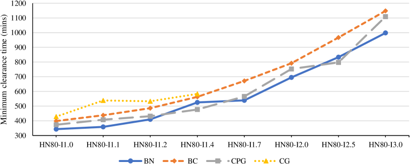
Figure 27: SUMO minimum clearance time without contraflow.

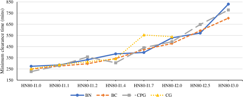
Figure 28: SUMO minimum clearance time with contraflow.

Instance	Normalized Minimum Clearance Time
	Without Contraflow				With Contraflow
	BN	BC	CPG	CG	BN	BC	CPG	CG
HN80-I1.0	1.32	1.19	1.33	0.94	1.41	1.11	1.13	1.07
HN80-I1.1	1.24	1.20	1.29	0.97	1.40	1.15	1.33	1.13
HN80-I1.2	1.37	1.23	1.31	0.94	1.48	1.14	1.52	1.10
HN80-I1.4	1.50	1.25	1.26	0.97	1.54	1.20	1.17	1.06
HN80-I1.7	1.33	1.26	1.27	-	1.37	1.26	1.38	0.96
HN80-I2.0	1.48	1.26	1.45	-	1.58	1.23	1.28	1.01
HN80-I2.5	1.45	1.26	1.28	-	1.41	1.25	1.47	-
HN80-I3.0	1.48	1.24	1.36	-	1.75	1.26	1.56	-
Average	1.40 $\pm$ 0.03	1.23 $\pm$ 0.01	1.32 $\pm$ 0.02	0.95 $\pm$ 0.01	1.49 $\pm$ 0.05	1.20 $\pm$ 0.02	1.36 $\pm$ 0.06	1.06 $\pm$ 0.03

Table 19: SUMO minimum clearance time normalized results.

Table 19 summarizes the normalized values for this setting. The table reveals statistically significant differences in the average normalized values of each method.

The CG method has normalized values which are closest to 1.0, followed by the BC, CPG, and BN methods. This indicates that the CG method produces minimum clearance times that are most reproducible in simulations, i.e., their times are the least optimistic and most accurately reflects what could be achieved in a real world setting. This is interesting since CG method is the only method that utilizes non-preemptive evacuation schedules. A possible rationale for this result is that the step response curves representing evacuation flow rates over time prevent the transportation network from being utilized to its full capacity systematically. Indeed, the flow rate is fixed to a constant value and cannot be increased to saturate available arc capacities at any given time unlike the flow rates of preemptive schedules. While this characteristic of the CG hampers its macroscopic performance, its conservative utilization of the transportation network has a positive side benefit in that it is less likely to cause congestion. The fact that the CG method’s normalized values are occasionally less than 1.0 warrants further explanation. This result is due to the discretization into 5 minute intervals in the time-expanded graph. This discretization forces travel time along each arc to be rounded up to the nearest 5 minute multiple when the arc is represented in the time-expanded graph, even though the actual travel time maybe less than this multiple. This quantization causes total travel times along an evacuation path to be a slight overestimate of actual times. In the simulation of other methods, this overestimation gets canceled out by congestion induced delays. However, the CG method produces flows that tend to under utilize the transportation network, which result in less congestion and delays. As such, the travel time overestimation does not get canceled out and is reflected in the normalized clearance times.

Method BC also produces normalized values close to 1.0. To understand why this was the case, it is useful to take a closer look at the visualizations of the simulations and, in particular, busy road intersections and to compare the congestion severity at these intersections for the the BN and CPG methods. Figures 29(a) and 29(b) show visualizations of the same intersection taken from simulations of the BC and BN methods respectively. The inspections reveal that even though congestion is present at these intersections in the BC simulations, it was consistently less severe than those of the other two methods. The BC method forces traffic flows at intersections to converge onto a single outgoing road. This limitation is not present in the other methods, which allow for convergent, divergent, and sometimes even crossing paths at any given intersection while often lead to more severe congestion. These observations support the normalized values obtained for the BC method which indicate its microscopic and macroscopic results are much closer.

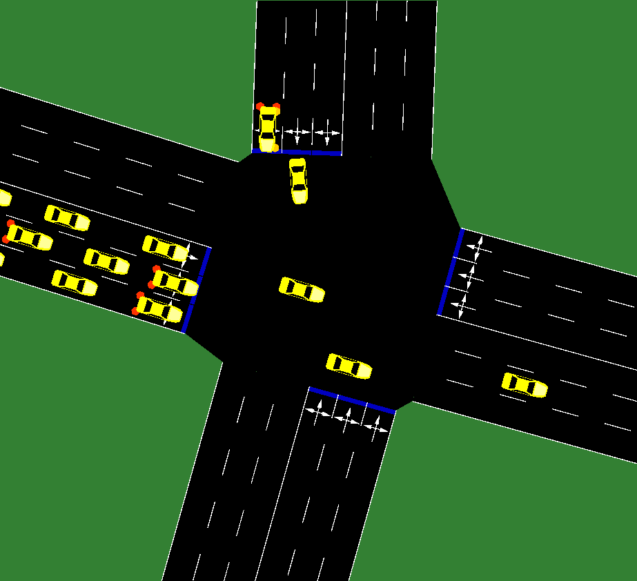
(a) Convergent traffic flow of BC method

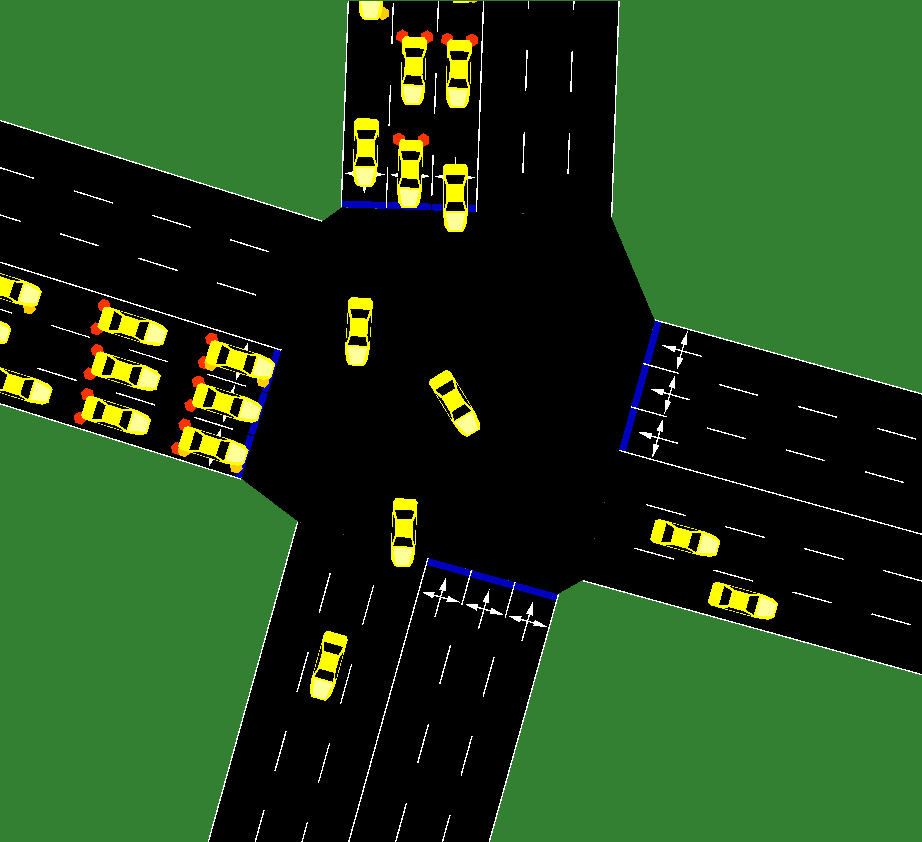
(b) Non-convergent traffic flow of BN method

Figure 29: Visualization of simulated traffic flow at an intersection produced by evacuaton plans of the BC and BN methods.

12 Perspectives

Extensions of the Optimization Algorithms

The macroscopic and microscopic evaluations contain two important findings:

1. Adding constraints on the evacuations, e.g., path convergence and non-preemption, increases the fidelity and overall effectiveness of the evacuation plans. In particular, for large population sizes, problems C-ZEPP and NP-ZEPP produce solutions which are dominated in macroscopic evaluations but become superior when validated in microscopic simulators.

2. Adding constraints on the evacuations may lead to more elegant optimization approaches. Indeed, problems C-ZEPP and NP-ZEPP are solved using exact Benders decomposition (method BC) and column generation (method CG), which is not the case of Problem ZEPP, which is approximated by methods BN and CPG. This elegance may, or may not, lead to improved computational performance: Method BC is the most efficient method studied in this paper but method CG is the most demanding.

An obvious direction for future work is to study convergent, non-preemptive zone-based evacuation planning. Enhancing method BC with non-preemption is not an easy task however. The subproblem becomes a complex scheduling problem that was studied in [11]. The key technical issue is to find effective combinatorial Benders cuts to link the subproblem and the restricted master problem. Method CG seems easier to extend with convergent paths, since they only affect the master problem. It remains to evaluate whether the resulting restricted master problem can be solved effectively.

Fidelity of the Macroscopic Approaches

This study demonstrated that macroscopic approaches such as methods BC and CG are of high fidelity: Their evacuation plans do not degrade in any significant way when evaluated with a microscopic simulator. This is an interesting finding on its own. Indeed, it indicates that, for the case study, it is not necessary to consider more complex models of the transportation network, such as the Cell Transmission Model (CTM) [8] which has raised significant interest due to its elegance and practicality in various settings. However, the CTM is a mixed integer formulation and hence it adds additional computational complexity to the models. Some work have considered the linear relaxation of the CTM: However, this linearization makes it possible to delay vehicles everywhere in the network, which is not practical in evacuations and makes the model overly optimistic.

Methods BN and CPG have been shown overly optimistic by the microscopic simulations. This is an important finding as well: It suggests that flow-based modeling of evacuations will also be significantly optimistic. Indeed, flow-based methods decide the route and timing of each individual evacuee and hence they have much more flexibility than zone-based evacuations. Similarly, methods not based on time-expanded graphs and not reasoning about time are unlikely to be of high fidelity in practice.

Evacuations Under Uncertainty

Moving from deterministic evacuation planning algorithms to optimization under uncertainty is a critical extension to the methods presented in this study. There are many sources of uncertainty in evacuations, from the natural or human-made disaster itself to evacuee compliance and potential accidents. Large-scale zone-based evacuation planning under uncertainty is largely unexplored. The work of Andreas and Smith [1] is a notable exception: They study a stochastic evacuation planning problems, where scenarios specify the uncertainty (e.g., the loss of an arc or an increased travel time). They assign penalties to each arc in the network and define the cost of a plan as the sum of the penalties on the arcs used in the evacuation. The resulting problem is to find a convergent evacuation plan that minimizes the expected cost. Andreas and Smith apply a Benders decomposition but their algorithm does not scale beyond a dozen nodes.

It is important to emphasize that, in evacuations, the uncertainty is not only exogenous (e.g., the flood may be more severe than expected): It also depends on the evacuation plan itself. Indeed, the probability of an accident along an arc increases with the flow being scheduled on the arc. This type of endogenous uncertainty is particularly difficult to handle efficiently.

Reliable Evacuation Plans

An interesting direction in evacuation planning is to borrow some ideas from power systems engineering and defines various notions of reliability. For instance, the dispatches of transmission systems satisfy a property known as n-1 reliability which means that the network can sustain the loss of a line or a generator and redispatch flows appropriately. Defining and finding n-1 reliable evacuation plans is an interesting avenue for further research. Within this framework, it would be typical to have a master problem to find a robust plan and a subproblem for each contingency. The subproblem will then aim at rerouting the flow of evacuees affected by the contingency without altering the rest of the evacuation significantly.

Evacuating Low-Mobility Population and Multi-Modal Evacuations

The problems studied in this paper assume that each evacuee (or each household) has a vehicle available for evacuation and do not consider low-mobility population. Bus evacuations (e.g., [4, 40, 15, 25, 9]) have been studied rather extensively for evacuating low-mobility population. It is important however to consider the multi-modal evacuations that integrate both vehicle owners and low-mobility population, since they share the same transportation network and may affect the design of contraflows. On-demand multimodal transit systems [31] may bring some significant benefits in that context, since these novel transit systems solve the first/last mile problem: They will be able to pick up riders at their location.

Additional Functionalities

There are a number of additional and critical issues that also deserve to be mentioned. The problem of reversed evacuations, i.e., bringing residents back to the evacuation area, is also of great importance and needs to take into account various cleaning efforts and priorities. The evacuation process itself should also take into account lodging and other amenities when scheduling an evacuation for a large area that will not be livable for a significant period of time. Taking into account these considerations may significantly reduce the financial burden of many families.

13 Related Work

A comprehensive survey of evacuation planning is available in [2]. The goal of this section is to not duplicate this survey but to provide some context for this study. The importance of prescriptive evacuations, in which evacuation is orchestrated by a central authority as opposed to self-evacuation, is well recognized in the field, making it the focal point of various studies.

As mentioned in the introduction, Hamacher and Tjandra [16] distinguishes between microscopic and macroscopic approaches to evacuation modeling. Microscopic approaches model individual characteristics of evacuees, their interactions with each other, and how these factors influence their movement. On the other hand, macroscopic approaches aggregates evacuees and models their movements as flow in a network. While all of the algorithms described This paper has presented macroscopic approaches that were evaluated using microscopic methods.

The majority of macroscopic approaches are flow-based: They solve the evacuation planning problem as a flow on a time-expanded graph. For instance, [29, 28] propose three heuristics to design an evacuation plan with multiple evacuation routes per evacuation node, minimizing the time of the last evacuation. They show that, in the best case, the proposed heuristic is able to solve randomly generated instances of up to 50,000 nodes and 150,000 edges in under 6 minutes. Liu et al. [27] propose a Heuristic Algorithm for Staged Traffic Evacuation (HASTE), whose main difference is the use of the CTM to capture more accurately the flow of evacuees. Lim et al. [26] consider a short-notice regional evacuation maximizing the number of evacuees reaching safety weighted by the severity of the threat. They propose two solution approaches to solve the problem, and present computational experiments on instances derived from the Houston-Galveston region (USA) with up to 66 nodes, 187 edges, and a horizon of 192 time steps. Bretschneider and Kimms [5, 6] focus on modeling more accurately the transportation network; they present a free-flow mathematical model over a detailed street network and include computational experiments on generated instances with a grid topology of up to 240 nodes, 330 edges, and considering 150 times steps.

Flow-based approaches are not zone-based and hence do not provide evacuation plans that comply with the procedures in place in most emergency services and local authorities. Assigning a routing and timing to every indivdual evacuee is unlikely to result in actionable plans. To the best of our knowledge, only a handful of studies design zone-based evacuation plans that produce both a set of evacuation routes and an evacuation schedule. Huibregtse et al. [20] propose a two-stage algorithm that first generates a set of evacuation routes and feasible evacuation times, and then assigns a route and time to each evacuated area using an ant colony optimization algorithm. The main difference with the present work is that the approach does not explicitly schedule the evacuation but relies on a third party simulator (EVAQ) to simulate the departure time of evacuees depending on the evacuation time decided for each area and evaluate the quality of the solution. In later work, the authors studied the robustness of the produced solution [19], and strategies to improve the compliance of evacuees [18]. Bish and Sherali [3] present a model based on a CTM that assigns a single evacuation path to each evacuation node but fixes a response curve for each zone. Computational results include instances with up to 13 evacuation nodes, 2 safe nodes, and 72 edges. The CPG and CG methods were originally proposed in [34] and [33] respectively. Even et al. [12] takes a different approach by introducing the Convergent Evacuation Planning Problem (CEPP) which aims at removing forks from all evacuation routes combined to eliminate delays caused by diverging and crossing routes. They propose a two-stage approach to solve the problem which separates route design and evacuation scheduling. Their work served as the foundation of the algorithm by Romanski and Van Hentenryck [36], one of the algorithms described in detail in this paper (method BC). As mentioned earlier, Andreas and Smith [1] considers a stochastic evacuation planning with convergent paths. Although not directly related, it is interesting to mention the work of Chen and Miller-Hooks [7] who provide an exact technique based on Benders decomposition to solve the Building Evacuation Problem with Shared Information. The problem is formulated as a MIP with shared information constraints to ensure evacuees departing from the same location at the same departure time receive common instructions and seeks to route evacuees from multiple locations in a building to exits such that total evacuation time is minimized.

14 Conclusion

This paper presented a systematic study large-scale zone-based evacuation planning, both from an effectiveness and a computational standpoint. In zone-based evacuation planning, the region to evacuate is divided into zones and each zone must be assigned a path to safety and departure times along the path. Zone-based evacuations are highly desirable in practice because they allow emergency services to communicate evacuation orders and to control the evacuation more accurately.

The paper reviewed several existing optimization algorithms, and presented new ones, and evaluated them, on a real, large-scale case study, both from a macroscopic standpoint and through microscopic simulations under a variety of assumptions. In particular, the paper evaluated the impact of contraflow, preemption, and convergent evacuations.

The main take-away is probably the success of mathematical programming for designing macroscopic evacuation planning algorithms that are effective when evaluated by microscopic simulators on large-scale scenarios. The algorithms thus provide both primal solutions and a performance guarantee. A second key take-away is the importance of constraining the optimization algorithms to produce realistic plans. By imposing the non-preemption constraints, the optimization algorithm produces evacuation plans that are easy to enforce and of high fidelity. By imposing convergence properties, the optimization algorithm avoid congestion and driver hesitations. The optimization algorithms have been shown to be highly practical and some of them can even be used in real-time settings.

The papers also listed a number of directions for future work and perspectives on the field. Perhaps the most pressing issues center around delivering plans that are robust under uncertainty and to support multimodal evacuations that evacuate both vehicle owners and low-mobility populations.

References

- [1] April K. Andreas and J. Cole Smith. Decomposition algorithms for the design of a nonsimultaneous capacitated evacuation tree network. Networks, 53(2):91–103, 2009.
- [2] Vedat Bayram. Optimization models for large scale network evacuation planning and management: A literature review. Surveys in Operations Research and Management Science, 2016.
- [3] Douglas R. Bish and Hanif D. Sherali. Aggregate-level demand management in evacuation planning. European Journal of Operational Research, 224(1):79 – 92, 2013.
- [4] D.R. Bish. Planning for a bus-based evacuation. OR Spectrum, 33(3):629–654, 2011.
- [5] S. Bretschneider and A. Kimms. A basic mathematical model for evacuation problems in urban areas. Transportation Research Part A: Policy and Practice, 45(6):523 – 539, 2011.
- [6] S. Bretschneider and A. Kimms. Pattern-based evacuation planning for urban areas. European Journal of Operational Research, 216(1):57 – 69, 2012.
- [7] Lichun Chen and Elise Miller-Hooks. The building evacuation problem with shared information. Naval Research Logistics (NRL), 55(4):363–376, 2008.
- [8] Carlos F. Daganzo. The cell transmission model: A dynamic representation of highway traffic consistent with the hydrodynamic theory. Transportation Research Part B: Methodological, 28(4):269 – 287, 1994.
- [9] T. Dhamala and I. Adhikari. On evacuation planning optimization problems from transit-based perspective. International Journal of Operations Research, 15(1):29–47, 2018.
- [10] Jakob Erdmann. SUMO’s Lane-Changing Model, pages 105–123. Springer International Publishing, Cham, 2015.
- [11] C. Even, A. Schutt, and P. Van Hentenryck. A Constraint Programming Approach for Non-Preemptive Evacuation Scheduling. In 21th International Conference on the Principles and Practice of Constraint Programming (CP-2015), Cork, Ireland, September 2015.
- [12] Caroline Even, Victor Pillac, and Pascal Van Hentenryck. Convergent plans for large-scale evacuations. In Proceedings of the Twenty-Ninth AAAI Conference on Artificial Intelligence, pages 1121–1127. AAAI Press, 2015.
- [13] L. R. Ford Jr. and D. R. Fulkerson. Flows in Networks. Princeton University Press, Princeton, New Jersey, 1962.
- [14] Michael R Gary and David S Johnson. Computers and Intractability: A Guide to the Theory of NP-completeness. W. H. Freeman and Company, San Francisco, California, 1979.
- [15] M. Goerigk, B. Gruen, and P. Hessler. Combining bus evacuation with location decisions: A branch-and-price approach. Transportation Research Procedia, 2:783–791, 2014.
- [16] H. W. Hamacher and S. A. Tjandra. Mathematical modelling of evacuation problems: A state of the art. Pedestrian and Evacuation Dynamics, pages 227–266, 2002.
- [17] Mohd. Hafiz Hasan and Pascal Van Hentenryck. A column-generation algorithm for evacuation planning with elementary paths. In Proceedings of the 23rd International Conference on Principles and Practice of Constraint Programming (CP-2017), Melbourne, Australia, August 2017.
- [18] Olga Huibregtse, Andreas Hegyi, and Serge P. Hoogendoorn. Blocking roads to increase the evacuation efficiency. Journal of Advanced Transportation, 46(3):282–289, 2012.
- [19] Olga L. Huibregtse, Michiel C.J. Bliemer, and Serge P. Hoogendoorn. Analysis of near-optimal evacuation instructions. Procedia Engineering, 3:189 – 203, 2010.
- [20] Olga L. Huibregtse, Serge P. Hoogendoorn, Andreas Hegyi, and Michiel C. J. Bliemer. A method to optimize evacuation instructions. OR Spectrum, 33(3):595–627, 2011.
- [21] Stefan Irnich and Guy Desaulniers. Shortest path problems with resource constraints. In Column Generation, pages 33–65. Springer, 2005.
- [22] Víctor M. Jiménez and Andrés Marzal. Computing the K Shortest Paths: A New Algorithm and an Experimental Comparison, pages 15–29. Springer Berlin Heidelberg, Berlin, Heidelberg, 1999.
- [23] Daniel Krajzewicz, Jakob Erdmann, Michael Behrisch, and Laura Bieker. Recent development and applications of SUMO - Simulation of Urban MObility. International Journal On Advances in Systems and Measurements, 5(3&4):128–138, December 2012.
- [24] Stefan Krauß. Microscopic Modeling of Traffic Flow: Investigation of Collision Free Vehicle Dynamics. PhD thesis, University of Cologne, 1998.
- [25] J. Lee, M. Li, J. Xu, L. Wei, X. Jia, and C. Sun. Modeling a risk-based dynamic bus schedule problem under no-notice evacuation incorporated with dynamics of disaster, supply, and demand conditions. Journal of Advanced Transportation, 1(23), 2019.
- [26] Gino J. Lim, Shabnam Zangeneh, M. Reza Baharnemati, and Tiravat Assavapokee. A capacitated network flow optimization approach for short notice evacuation planning. European Journal of Operational Research, 223(1):234 – 245, 2012.
- [27] Henry X Liu, Xiaozheng He, and Xuegang Ban. A cell-based many-to-one dynamic system optimal model and its heuristic solution method for emergency evacuation. In Proc. 86th Annual Meeting Transportation Res. Board, pages 1–20, 2007.
- [28] Qingsong Lu, Betsy George, and Shashi Shekhar. Capacity Constrained Routing Algorithms for Evacuation Planning: A Summary of Results, pages 291–307. Springer Berlin Heidelberg, Berlin, Heidelberg, 2005.
- [29] Qingsong Lu, Yan Huang, and Shashi Shekhar. Evacuation Planning: A Capacity Constrained Routing Approach, pages 111–125. Springer Berlin Heidelberg, Berlin, Heidelberg, 2003.
- [30] Thomas Magnanti and Richard Wong. Accelerating benders decomposition: Algorithmic enhancement and model selection criteria. Operations Research, 29(3):464–484, 1981.
- [31] Arthur Maheo, Phlip Kilby, and Pascal Van Hentenryck. Benders Decomposition for the Design of a Hub and Shuttle Public Transit System. Transportation Science, 53:77–88, January–February 2019.
- [32] Adam J. Pel, Michiel C. J. Bliemer, and Serge P. Hoogendoorn. A review on travel behaviour modelling in dynamic traffic simulation models for evacuations. Transportation, 39(1):97–123, 2012.
- [33] Victor Pillac, Manuel Cebrian, and Pascal Van Hentenryck. A column-generation approach for joint mobilization and evacuation planning. Constraints, 20(3):285–303, 2015.
- [34] Victor Pillac, Pascal Van Hentenryck, and Caroline Even. A conflict-based path-generation heuristic for evacuation planning. Transportation Research Part B, 83:136–150, 2016.
- [35] Red Cross. World disasters report 2010–focus on urban risk. International Federation of Red Cross and Red Crescent Societies, Geneva, 2010.
- [36] Julia Romanski and Pascal Van Hentenryck. Benders decomposition for large-scale prescriptive evacuations. In Proceedings of the Thirtieth AAAI Conference on Artificial Intelligence, pages 3894–3900. AAAI Press, 2016.
- [37] Gregoris Theodoulou and Brian Wolshon. Alternative methods to increase the effectiveness of freeway contraflow evacuation. Transportation Research Record: Journal of the Transportation Research Board, 1865:48–56, 2004.
- [38] Frances Fragos Townsend et al. The federal response to hurricane katrina: Lessons learned. Washington, DC: The White House, 2006.
- [39] Brian Wolshon. “One-way-out”: Contraflow freeway operation for hurricane evacuation. Natural Hazards Review, 2(3):105–112, 2001.
- [40] Hong Zheng. Optimization of bus routing strategies for evacuation. Journal of Advanced Transportation, 48(7):734–749, 2014.