Shear thinning and thickening in spherical nanoparticle dispersions

Abstract

We present a molecular dynamics study of the flow of rigid spherical nanoparticles in a simple fluid. We evaluate the viscosity of the dispersion as a function of shear rate and nanoparticle volume fraction. We observe shear thinning behavior at low volume fractions, as the shear rate increases, the shear forces overcome the brownian forces, resulting in more frequent and more violent collisions between the nanoparticles. This in turn results in more dissipation. We show that in order to be in the shear thinning regime the nanoparticle have to order themselves into layers longitudinal to the flow to minimize the collisions. As the nanoparticle volume fraction increases there is less room to form the ordered layers, consequently as the shear rate increases the nanoparticles collide more which results in turn in shear thickening. Most interestingly, we show that at intermediate volume fractions the system exhibits metastability, with successions of ordered and disordered states along the same trajectory. Our results suggest that for nanoparticles in a simple fluid the hydro-clustering phenomenon is not present, instead the order-disorder transition is the leading mechanism for the transition from shear thinning to shear thickening.

I Introduction

Viscosity is one of the fundamental physical property of fluids. It defines a fluid’s resistance to flow. The phenomenological law relating the shear stress to the shear rate is Newton’s law of viscosity Katz (2010),

$$\tau=\eta(\dot{\gamma})\ \dot{\gamma},$$ (1)

where $\tau$ is the shear stress, $\dot{\gamma}=\partial v_{x}/\partial z$ the shear rate, and $\eta$ the shear viscosity. Shear viscosity quantifies the rate of momentum transfer per unit area between two adjacent layers of fluid. A large viscosity results in higher momentum transfer, at the limit $\eta\to\infty$ the system behaves like a solid and all the momentum is transferred. For the so-called Newtonian fluids, the shear viscosity is independent of the shear rate. Most fluids are Newtonian for small shear rates, the so-called newtonian plateau. However, many fluids show non-Newtonian behavior at higher shear rates, usually one observes a decreasing viscosity with increasing shear rate. The fluid flows easier as it becomes faster. This phenomenon is called shear-thinning and is observed in fluids such as polymer meltsDoi and Edwards (1986); Han (2007), colloid or non-colloids dispersions Brown and Jaeger (2014); Bounoua et al. (2016) and even nano-confined water Kapoor, Amandeep, and Patil (2014).

On the other hand, some fluids exhibit the opposite behaviour, after a critical shear rate, $\dot{\gamma}_{c}$, flow becomes more difficult, viscosity increases, this is called shear-thickening. Shear-thickening is generally observed in suspensions and colloidal dispersions Barnes (1989); Brown and Jaeger (2014); Crawford et al. (2013). At high volume fractions of colloids and high shear rates, shear-thickening can lead to a diverging viscosity. This was observed in in early experiments with suspensions of spherical particles by HoffmanHoffman (1972, 1974, 1991), spherical colloid dispersions by Bender and Wagner Bender and Wagner (1996) and recently in cornstarch suspensions by Madraki et al. Madraki et al. (2017).

Shear-thickening can have negative impacts on engineering and industrial applications of materials such as cement or coating dyes Maybury, Ho, and Binhowimal (2017); Khandavalli and Rothstein (2016). However, it can also be a useful property, for example for the fabrication of soft armors Lee, Wetzel, and Wagner (2003); Gong et al. (2014) or sound insulation Li et al. (2014). In either case, it is important to have an understanding of the microscopic dynamics leading to shear-thickening. Shear-thickening depends on several parameters. Primarily the volume fraction of solid particles, $\phi$. Indeed, experiments Jiang et al. (2014); Chow and Zukoski (1995); Fall et al. (2015); Cwalina, Harrison, and Wagner (2016) and simulations Foss and Brady (2000); Seto et al. (2013a); Mari et al. (2015); Pednekar, Chun, and Morris (2017) show that shear-thickening occurs only after a minimum volume fraction of particle is reached in the fluid. The size of the particles is an other important parameter. It affects the critical shear rate, the larger the particles are the smaller is $\dot{\gamma}_{c}$, thus the onset of thickening is at lower values of the shear rate Maranzano and Wagner (2001); Li et al. (2017). The interaction between the fluid and solid particles is also of importance. Indeed, if the particle-fluid interaction is too repulsive –or the particle-particle interaction too attractive– the solid particles will tend to aggregate, consequently the fluid will loose its characterization of suspension or dispersion, and become unstable. The rheology of aggregating fluids is another area of research Wolthers et al. (1996).

The shear thickening phenomenon is divided into two classes, discontinuous shear thickening (DST) for which the viscosity increases of several order of magnitudes. DST occurs over a critical volume fraction of particles Seto et al. (2013a). DST is now relatively well understood, it is caused by frictional contact between the suspended particles Peters, Majumdar, and Jaeger (2016) which can eventually lead to a jamming state Fall et al. (2008); Brown et al. (2010). The second mechanism is called continuous shear thickening (CST) where viscosity increases slowly. Two alternative mechanisms for CST were proposed. First the so-called order-disorder transition (ODT) suggested by Hoffmann Hoffman (1972, 1998) . The experiments on concentrated colloidal suspensions suggested that shear-thickening occurs when the suspension has a transition from an ordered micro-structure to a disordered one. Later experiments by Ackerson and Pusey Ackerson and Pusey (1988) Yan et al. Yan et al. (1994) also observed the formation of ordered layers or strings of colloids. At low shear rates the suspended particles flow in ordered layers while at high shear rates their flow becomes disordered. This results in increased collisions and consequently increased frictional interactions and eventually shear thickening.

The second mechanism is the so-called hydro-clustering phenomenon. Hydro-clusters were first observed by Brady and Bossis Brady and Bossis (1985) in Stokesian dynamics simulations, later experimental evidences were observed by Wagner and coworkersMaranzano and Wagner (2002); Kalman and Wagner (2009) and Cheng et al.Cheng et al. (2011). The results suggests that for large shear rates, the forces due to the flow overwhelms the repulsive forces between the solid particles. This results in the formation of transient clusters. The lubrication forces acting on the interstitial fluid causes an increased dissipation and consequently larger viscosity. As the shear rate increases the size of the clusters increase, resulting in shear thickening.

The aim of this paper is to elucidate which mechanism is relevant for dispersions of spherical nanoparticles. To achieve this we model a suspension of nanoparticles with coarsed-grained molecular dynamics simulations.

The manuscript is organized as follows: In Sec. II we describe our simulation model and technique. Then, in Sec. III, we compute the viscosity as a function of shear rate for different volume fractions of nanoparticles. We relate the thinning or thickening behavior of the fluid to the microscopic structure of the fluid where we show that at large volume fractions thinning occurs when the nanoparticles can order themselves in order to minimize the number of collisions. The manuscript closes with a brief discussion in Sec. IV

II The Model

In this work we are interested in the universal properties leading to thinning or thickening in suspensions. We thus construct a coarse-grained model. The particles of the base fluid interact through a Lennard-Jones (LJ) potential,

$$V_{LJ}=\left\{\begin{array}[]{ccc}4\epsilon\left[(\frac{\sigma}{r})^{12}-(\frac{\sigma}{r})^{6}\right]&{\rm for}&r<r_{c}\\ 0&{\rm for}&r\geq r_{c}\end{array}\right.$$ (2)

where the cutoff distance is chosen to be $r_{c}=2.5\sigma$. The Lennard-Jones parameters are fixed to unity, $\epsilon=1$ and $\sigma=1$. The mass of the particles is also fixed to unity $m=1$. A unit of time can thus be expressed as $\tau=\sigma\sqrt{m/\epsilon}$. The nanoparticles are modeled as rigid molecules of spherical shape with a radius of 1 $\sigma$. They consist of 100 atoms, which is enough to ensure fluid atoms can not enter inside them. The interactions between the nanoparticles and the fluid, and between the nanoparticles is modelled with a modified Lennard-Jones potential in order to control the hydrophobicity of the nanoparticles,

$$V_{ab}=\left\{\begin{array}[]{ccc}4\epsilon\left[(\frac{\sigma}{r})^{12}-C_{ab}(\frac{\sigma}{r})^{6}\right]&{\rm for}&r<r_{c}\\ 0&{\rm for}&r\geq r_{c}\end{array}\right.$$ (3)

$a,b$ indicates the type of atom, $f$ for fluid atoms and $n$ for atoms of nanoparticles. The parameter $C_{ab}$ controls the strength of the attractive part. $C_{nn}=0.2$ and $C_{nf}=0.5$ permits to have a well dispersed nanofluid.

The volume fraction of nanoparticles in the suspension can be written as,

$$\phi=N_{p}\frac{\frac{4}{3}\pi r_{p}^{3}}{V}$$ (4)

where $r_{p}$ is the effective radius of the nanoparticle, $N_{p}$ the number of nanoparticles and $V$ is the volume of the simulation box. The effective radius of the nanoparticle can be evaluated thanks to the radial pair correlation function evaluated between the nanoparticles and nanoparticles, and nanoparticles and the fluid as depicted in Fig. 1

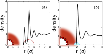
Figure 1: (a) Pair correlation function between nanoparticles, the dashed line represents a nanoparticle at the most probable separation, the blurred region corresponds to the effective size of a nanoparticle, approximately $2\ \sigma$. (b) Pair correlation between nanoparticles and fluid atoms, the dashed line represents a fluid atom at its most probable distance to the nanoparticle.

Considering the radial distribution, we define the effective radius of the nanoparticle as $2\ \sigma$. The volume fractions are evaluated with this value. Notice that according to Fig. 1(a) the most probable distance of two nanoparticles is approximately $4\ \sigma$. Finally, we prepare cubical simulation boxes with $16\ \sigma$ of side length. The nanoparticle volume fraction varies between $\phi=0$ to $\phi=0.53$. This corresponds to a number of fluid atoms varying between 3648 and 1708, and 0 to 65 nanoparticles. We depict a typical system in Fig. 2.

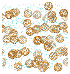
Figure 2: Snapshot of a suspension of spherical nanoparticles with a volume fraction 0.41 dispersed in a Lennard-Jones fluid.

II.1 Equations of motion

We use the rotation matrix algorithm to enforce the rigid body motion. Dullweber, Leimkuhler, and McLachlan (1997); Rapaport (2004) While the SHAKE or RATTLE Ryckaert, Ciccotti, and Berendsen (1977); Andersen (1983) algorithms use constraints to enforce the rigid body motion, it is not the case for the rotation matrix algorithm Sunarso, Tsuji, and Chono (2011); Akimov and Kolomeisky (2011); Orsi, Michel, and Essex (2010). One can thus derive a reversible integration algorithm which in turn permits to do long simulations without any unphysical velocity scalings.

The rotation matrix is the transformation that maps the moment of inertia tensor in the simulation box frame of the molecule to the frame in which the moment of inertia tensor is diagonal (principal axes frame). At every time step the rotation matrix of each molecule is calculated, and the coordinates are transformed into the principal axes frame, in which the equations of motions are,

$$\dot{\bm{r}}_{\rm CM} = \frac{\bm{p}_{\rm CM}}{M}$$ (5)

$$\dot{\bm{p}}_{\rm CM} = \sum\mathbf{F}_{i}$$ (6)

$$\dot{\bm{\theta}} = \bm{\omega}$$ (7)

$$\bm{I}\dot{\bm{\omega}} = \sum\bm{\tau}_{i}$$ (8)

where the moment of inertia matrix $\bm{I}$ is now diagonal and constant. $M$ is the mass of the molecule, $\bm{r}_{\rm CM}$ and $\bm{p}_{\rm CM}$ respectively, the position of its center of mass and its momentum. Finally, $\bm{\theta}$ and $\bm{\omega}$ are respectively the angular position and angular velocity vectors of the molecule. The total force and torque is calculated over all the interactions with fluid atoms and atoms of other molecules. Angular accelerations, angular velocities, positions and momenta of the center of mass are updated with a velocity Verlet type scheme in the principal axes frame, then the coordinates are transformed back to the simulation box frame.

In order to compute the viscosity as a function of shear rate we impose a Couette flow on the fluid. One can achieve a Couette flow either by adding a physical wall to the system and give is a constant velocity a motion, or by changing the boundary conditions for the bulk fluid in order to avoid surface effects. For the latter one must use the Lee-Edwards or sliding brick periodic boundaries Lees and Edwards (1972). The modification of the periodic boundaries leads to a change in the equations of motion. For point particles one can use the isokinetic SLLOD algorithm Edberg, Morriss, and Evans (1987); Travis, Daivis, and Evans (1995); Evans and Morriss (2008). The equations of motion for a Couette flow in the $\hat{x}$ direction are written as,

$$\dot{\mathbf{r}} = \frac{\mathbf{p}}{m}+\dot{\gamma}z\ \hat{x}$$ (9)

$$\dot{\mathbf{p}} = \mathbf{F}-\dot{\gamma}p_{z}\ \hat{x}-\zeta\mathbf{p}$$ (10)

where $\mathbf{F}$ is the total force exerted on the atom and $-\zeta\mathbf{p}$ a frictional term to achieve a constant kinetic energy simulation. For molecules one must use this algorithm with care. Indeed, the equations of motion in Eqs. 9 and 10 can only be applied to a mono-atomic fluid. For molecules they have to be modified to avoid the independent motion of atoms in a molecule. There are two possible approaches, atomic SLLOD and molecular SLLOD Edberg, Morriss, and Evans (1987); Travis, Daivis, and Evans (1995). The atomic SLLOD equations of motion are the same as the original except that a constraint is added to conserve the molecular structure. On the other hand, in the case of molecular SSLOD, the SSLOD algorithm is only applied to the center of mass of the molecule, hence avoiding the use of constraints. Both algorithms give the same results as long as the shear rate is not too large. The equations of motion for the center of mass of a molecule are thus,

$$\dot{\mathbf{r}}_{{\rm CM}} = \frac{\mathbf{p}_{{\rm CM}}}{M}+\dot{\gamma}z_{CM}\ \hat{x}$$ (11)

$$\dot{\mathbf{p}}_{{\rm CM}} = \mathbf{F}_{\rm CM}-\dot{\gamma}p_{{\rm CM}z}\ \hat{x}$$ (12)

where $\mathbf{F}_{\rm CM}$ is the total force acting on the molecule. Remark that the frictional term $-\zeta\mathbf{p}$ is not present for the molecules, since the number of fluid atoms is much larger than the number of molecules, thermalization is quickly achieved only with the fluid atoms.

II.2 Evaluation of the shear viscosity

One can evaluate the shear viscosity with equilibrium molecular dynamics (MD) thanks to the Green-Kubo relationship,

$$\eta=\beta V\int_{0}^{\infty}dt\ \langle P_{xz}(t)P_{xz}(0)\rangle$$ (13)

where $\beta$ is the inverse temperature, $V$ the volume of the system, and $P_{xz}$ the $xz$ component of the pressure tensor. On the other hand, for non-equilibrium molecular dynamics simulations (NEMD) one gets the viscosity directly from Newton’s law of viscosity,

$$\eta=-\frac{\langle P_{xz}\rangle}{\dot{\gamma}}.$$ (14)

Calculating the viscosity both from equilibrium MD and NEMD permits to validate the NEMD algorithm. The $xz$ component of the atomic pressure tensor is written as McQuarrie (1976),

$$P^{a}_{xz}=\frac{1}{V}\left(\sum_{i}\frac{p_{xi}\ p_{zi}}{m_{i}}+\sum_{i<j}F_{xij}z_{ij}\right)$$ (15)

Where the momentum is the usual momentum for equilibrium simulations, or in case of the SLLOD equations of motion they have to be taken as the peculiar momenta Edberg, Morriss, and Evans (1987); Travis, Daivis, and Evans (1995); Evans and Morriss (2008) which correspond to the thermal velocities, in other words independent from the shear applied to the system. This expression can be used for the Lennard-Jones fluid, however, the atoms of molecules do not have individual peculiar momenta because of the rigidity of molecules . For molecules, one must consider the molecular pressure tensor Edberg, Morriss, and Evans (1987); Travis, Daivis, and Evans (1995) which is determined in terms of the of peculiar momenta of the center of mass of the molecules and intermolecular forces acting on their center of mass,

$$P^{m}_{xz}=\frac{1}{V}\left(\sum_{i}\frac{p_{{\rm CM},xi}\ p_{{\rm CM},zi}}{M_{i}}+\sum_{i<j}F_{{\rm CM},xij}z_{{\rm CM},ij}\right)$$ (16)

Remark that while the atomic pressure tensor has to be symmetric, it is not the case for the molecular pressure tensor. The atomic and molecular pressure tensors are compared theoretically and computationally in Refs. Allen (1984); Edberg, Morriss, and Evans (1987); Travis, Daivis, and Evans (1995). They are related to each other as

$$P^{a}=P^{m}_{(S)}+\frac{1}{2}\ddot{\chi}$$ (17)

where the subscript $(S)$ denotes the symmetrized molecular pressure tensor and $\chi$ is written as

$$\chi=\sum_{i\alpha}m_{i\alpha}\delta\mathbf{r}_{i\alpha}\delta\mathbf{r}_{i\alpha}$$

where $\delta\mathbf{r}_{i\alpha}=\mathbf{r}_{i\alpha}-\mathbf{r}_{{\rm CM},i}$. Where $i$ is the index of the molecule and $\alpha$ is the index of the atom in the molecule. $\langle\ddot{\chi}\rangle=0$ for a system in a steady state. One can consequently use the symmetrized molecular pressure tensor to evaluate the viscosity.

The viscosity of the dispersion is evaluated from the hybrid pressure tensor which is the sum of the atomic pressure tensor in Eq. (15) and the symmetrized molecular pressure tensor in Eq. (16) for our mixture of point-like atoms and spherical nanoparticles.

III Results

III.1 Viscosity as a function of shear rate and volume fraction

Starting from a pure Lennard Jones fluid, we evaluate the viscosity of dispersions with different volume fractions $\phi$ as a function of the shear rate, for values in the range $\dot{\gamma}=0\ 1/\tau$ to $\dot{\gamma}=2\ 1/\tau$. Unfortunately, we can not compute higher values of the shear rate with the present algorithm. Indeed, the molecular SLLOD algorithms breaks down at very high shear ratesEdberg, Morriss, and Evans (1987); Travis, Daivis, and Evans (1995).

The simulations are performed with $10^{6}$ integration step with a time step $\Delta t=10^{-3}\tau$ after an equilibrium process which ensures the system has reached a non-equilibrium steady state. For shear rates smaller than $\dot{\gamma}=0.08\ 1/\tau$ the integrations run ten times longer to reduce the statistical error. All the simulations are carried out at the temperature $k_{B}T=1.2\epsilon$. We depict the results in Fig. 3.

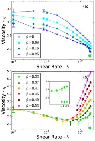
Figure 3: Viscosity $\eta$ as a function of the shear rate $\dot{\gamma}$ for different volume fraction of nanoparticles. (a) small volume fractions exhibiting shear thinning, (b) large volume fractions exhibiting shear thickening. The arrows indicate the beginning of the shear-thickening regime. The horizontal lines at low shear rates correspond to the Green-Kubo results. The diamonds in (a) represent the viscosity for $\phi=0.33$ in the thinning regime while the dashed line in (b) depicts the separation to the thinning regime. The inset of (b) represents a close up view on the bifurcation for the intermediate volume fraction $\phi=0.33$. The error bars correspond to the statistical error on an average with correlated sample. The solid lines serve as a guide to eye.

We observe that for small shear rates, the NEMD results are in agreement with the viscosity obtained from the equilibrium molecular dynamics simulations thanks to the Green-Kubo relationship. As the shear rate increases we observe two different behaviors, at low volume fractions, namely about $\phi=0.3$ the fluid exhibits shear thinning as depicted in Fig. 3(a). While for higher volume fractions shear thickening occurs after a critical shear rate value $\dot{\gamma}_{c}$ denoted by the arrows in Fig. 3(b). We observe that the critical shear rate decreases as the volume fraction increases. For volume fractions larger than $\phi=0.49$ the nanoparticle and liquid mixture form a solid for small shear rates, the fluid is in a jammed state. A steady state Couette flow can only be formed for large enough shear rates. Finally, the most interesting behavior is for the intermediate volume fraction $\phi=0.33$, after the shear thinning regime a bifurcation occurs. Along the same trajectory we observe sequences of thinning regime and thickening regime. Our simulation suggest the duration of each sequence is random, however the thinning states appears to become longer with increasing shear rate. In order to elucidate this metastable behaviour one has to study the microstructure of the fluid.

III.2 Microscopic structure

In order to understand what happens at the microscopic scale to the dispersions in the different viscosity regimes we evaluate the two-dimensional pair correlation functions of the nanoparticles. The two-dimensional pair correlation function is found by first evaluating the pair correlation function in three dimensions between nanoparticles. The result is then averaged over the $y$ direction and over all the nanoparticles. We depict in Fig. 4 the two-dimensional pair correlation function for two different volume fractions of nanoparticles, one which exhibits shear thinning, $\phi=0.25$, and the other shear thickening, $\phi=0.45$. We evaluate the correlation function for increasing values of the shear rate.

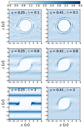
Figure 4: Two dimensional pair correlations for volume fractions $\phi=0.25$ and $\phi=0.41$ for different shear rates. Darker regions correspond to regions of higher density.

For small values of the shear rate both volume fractions exhibit shear thinning, their pair correlation functions are also similar, in both case the fluid is isotropic. However, as the shear rate increases, the pair correlation for $\phi=0.25$ shows a different behavior. One observes that layers appear and become more apparent with increasing shear rate. The distance between the layers is approximately $4\ \sigma$, which corresponds to the most probable distance between two nanoparticles as depicted in Fig. 1(b). As the shear rate increases the nanoparticles follow trajectories in which they avoid each other by forming a layered micro structure. It should be noted that those layers are the result of statistical averages and are not apparent when we analyze a single snap shot of the simulation. Similar layers called sliding layers were observed experimentally previously Yan et al. (1994); López-Barrón, Wagner, and Porcar (2015); Lee et al. (2018). As the shear rate increases, the nanoparticles tend to move in layers, hence avoiding collisions. This results in less energy dissipation, and thus decreased viscosity. For $\phi=0.45$ no such layers are formed, the nanoparticles can undergo violent collisions, which in turn increases the viscosity of the dispersion.

We now focus on the intermediate volume fraction $\phi=0.33$ which exhibits a metastable behavior at high enough shear rates. We depict in Fig. 5 the two dimensional pair correlation functions in the thinning and thickening regime and the shear stress as a function of time.

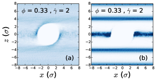
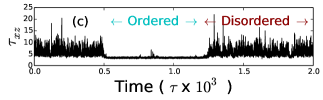
Figure 5: Two dimensional pair correlations for the intermediate volume fractions $\phi=0.33$ for the thickening regime (a) and thinning regime (b). (c) depicts the shear stress $\tau_{xz}$ as a function of time.

We observe that along the same trajectory the system is first in a disordered state, in which the shear stress is high and as a consequence the viscosity. After a while the nanoparticles order themselves for some finite duration thus decreasing the viscosity significantly. This process repeats at random intervals, hence suggesting the ordered state is metastable, large enough fluctuations can disrupt the layers.

In order to quantify the layering inside the fluid we evaluate the power spectrum in the $z$ direction and depict its value for $z=4\ \sigma$ as a function of shear rate in Fig. 6.

We see that for systems exhibiting shear thinning, the amplitude of the mode corresponding to the layer width increases very fast with the shear rate while systems undergoing shear thickening remain isotropic. Remark that the ordering increases continuously, we can not define a specific shear rate at which ordering starts. In general, as the volume fraction increases the layering becomes more pronounced, this is due to the fact that there are more nanoparticles in the layers, and thus a larger density.

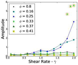
Figure 6: Amplitude of the power spectrum in the transverse direction to the flow at $z=4\ \sigma$ as a function of shear rate. The circles indicate the intermediate volume fraction $\phi=0.33$ in the thinning regime.

This behavior is typical of the order-disorder transition phenomenon proposed by Hoffman Hoffman (1991, 1998), as the shear rate changes micro structures are formed by the nanoparticles to avoid the increase in internal stress and as a consequence shear thickening. We remark that at very low volume fractions the nanoparticles have very few interactions, as a consequence they do not need to form sliding layers to decrease the internal stress. The layers occur at high volume fractions and large enough shear rates.

On the other hand, our results do not suggest hydro-clusters are formed in the shear thickening regime. Instead the nanoparticles remain well dispersed. We believe that for nanoparticles the absence of surface roughness, and thus macroscopic frictional effects prevents the formation of transient clusters. It is interesting to see that for nanoparticles, the shear-thickening phenomenon does not require hydro-clusters to form as suggested by several authors Pan et al. (2015); Guy, Hermes, and Poon (2015); Mari et al. (2014); Heussinger (2013); Seto et al. (2013b); Denn, Morris, and Bonn (2018); Fernandez et al. (2013).

III.3 Nanoparticle collisions

In this section we analyze the effect of nanoparticle-nanoparticle collisions on the viscosity. A collision between two nanoparticles is defined as an interaction in which two atoms of the nanoparticles are closer than $1\ \sigma$, which corresponds to the repulsive part of the interaction potential. We depict in Fig. 7(a) the number of collisions per frame averaged over all the frames.

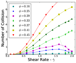
Figure 7: Average number of nanoparticle collisions per frame as a function of shear rate for different volume fractions. The dashed line indicate the bifurcation for the intermediate volume fraction. The solid lines serve as a guide to eye.

At equilibrium and low shear rates the repulsive part of the Lennard-Jones potential does not allow particles to get too close, thus the number of collisions is small. Moreover, if the volume fraction in nanoparticles is small, the probability of finding two nanoparticles in the same neighborhood is small and thus very few collisions occur. As the shear rate increases, the increased stress results in more and more nanoparticle collisions. At the same time we observe the collisions become more violent with a larger repulsive force on average, thus resulting in a larger energy dissipation and viscosity.

However, we notice that for the volume fractions exhibiting shear thinning as the shear rate increases the number of collisions decreases. This observation is in agreement with the formation of the sliding layers in systems exhibiting shear thinning. The layers permit the nanoparticles to avoid colliding, and as a consequence the overall dissipation is reduced and with it the shear viscosity. For the intermediate volume fraction $\phi=0.33$ we observe the same behavior as the previous results, the number of collisions bifurcates into two solutions, either a large number of collisions in the disordered state either a low number in the ordered one. We must point out that we did not observe any collisions involving more than two nanoparticles in our simulations, the only events are pairs of nanoparticle colliding, as a consequence we can not attribute the increase in interactions to the formation of hydroclusters.

IV Conclusion

We can summarize the results of the previous sections in a phase diagram as depicted in Fig. 8.

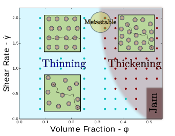
Figure 8: Phase diagram of the flow characteristic as a function of shear rate and volume fraction. The circles represent simulation points.

At low volume fractions the nanoparticles are disordered and shear thinning is observed, as the shear rate increases the nanoparticles start to form layers in order to minimize collisions, and consequently shear thinning is observed. As the volume fraction is further increased we observe a metastable region where the nanoparticles go through successions of ordered and disordered phases. The simulations suggest that the duration of the ordered state increases with shear rate however further research should be carried out. When the volume fraction is increased further, there is not enough room for the nanoparticles to form an ordered state, this in turn results in shear thickening. Finally, for very high volume fraction we observe a jammed state at low shear rates, the fluid behaves as a solid, shear flow is only possible after a sufficiently large shear rate is applied.

Our simulations suggest that for a dispersion of spherical nanoparticles in a simple fluid shear thickening is the result of the increased collisions, and therefore energy dissipation. While for low shear rates, hydrodynamic and Brownian forces are not enough to push the dispersed molecules into the repulsive part of the interaction potential, the high shear rates force the nanoparticles to collide. The commonly accepted mechanism of hydro-clustering Pan et al. (2015); Guy, Hermes, and Poon (2015); Mari et al. (2014); Heussinger (2013); Seto et al. (2013b); Denn, Morris, and Bonn (2018); Fernandez et al. (2013) is not the leading mechanism for shear thickening in the dispersion of spherical nanoparticles we consider in this study. We believe that one should consider larger colloids–at scales of micrometers instead of nanometers– so that surface asperities and friction would contribute to their formation. On the other hand, at high volume fractions the leading mechanism for the transition from thinning to thickening corresponds to the order-disorder transition previously suggested by Hoffman Hoffman (1972, 1998). Our study suggests that there is no single explanation for the shear thinning to thickening transition, different mechanisms become dominant depending on the scale of the colloids. However, the simple numerical model we propose permit to have a microscopic understanding of the phenomenon.