Robust Kalman Filtering with Probabilistic Uncertainty in System Parameters

Abstract

In this paper, we propose a robust Kalman filtering framework for systems with probabilistic uncertainty in system parameters. We consider two cases, namely discrete time systems, and continuous time systems with discrete measurements. The uncertainty, characterized by mean and variance of the states, is propagated using conditional expectations and polynomial chaos expansion framework. The results obtained using the proposed filter are compared with existing robust filters in the literature. The proposed filter demonstrates better performance in terms of estimation error and rate of convergence.

I Introduction

Robust filtering algorithms such as $\mathcal{H}_{2}/\mathcal{H}_{\infty}$ filters and robust Kalman filters, have been developed to address uncertainty in system models. In the $\mathcal{H}_{2}$/$\mathcal{H}_{\infty}$ framework, filters are designed to minimize the impact of exogenous signals, i.e. process and sensor noise, on the estimation error [1, 2, 3, 4, 5]. A robust Kalman filter is an extension of the well known Kalman filter, which can handle uncertainties in the system [6]. In this framework, the filter is designed to minimize an upper bound on the estimation error variance [7, 8, 9, 10, 11, 12], or the worst-case error variance [13, 14, 15]. Our work falls in the category of robust Kalman framework.

Existing robust Kalman filter algorithms can be categorized based on how system uncertainty is represented, which is assumed to be parametric. The uncertainty is either represented as norm bounded parameter uncertainty [6, 7, 8, 9, 10, 11, 12], or polytopic parametric uncertainty [16, 5]. In this work, we model parametric uncertainty as random variables with known probability density function (PDF). To the best of our knowledge, this is the first work on robust Kalman filtering with probabilistic system uncertainty.

We present two robust Kalman filtering algorithms with probabilistic uncertainty in system parameters. The first algorithm is for discrete-time (DT) system where the dynamics and measurements are both in discrete time. The second algorithm is for continuous-time (CT) dynamical systems with discrete-time measurements. In both these cases, mean and variance of uncertain states are calculated using a formulation based on conditional expectation. For the CT system, we apply polynomial chaos (PC) framework which provides a deterministic and computationally tractable approach to propagate the uncertainty.

The rest of the paper is organized as follows. We first present the problem formulation with uncertainty in CT and DT domain in §II followed by a discussion on polynomial chaos framework in §III. §IV presents the proposed robust filter. Simulation results are presented in §V followed by concluding remarks in §VI.

II Problem Formulation

The objective of filtering is to estimate the state-trajectory $\boldsymbol{x}(t)$ or $\boldsymbol{x}_{k}$ of a physical process in CT or DT, given noisy measurements. The uncertainty in the system parameters, in the external excitation (process noise), and in the measurement errors (sensor noise), are all treated as probabilistic. The model for the evolution of the state is assumed to be the following linear-time-varying stochastic system,

CT: $${\dot{\boldsymbol{x}}(t)=\boldsymbol{A}({\boldsymbol{\Delta}}_{k-1})\boldsymbol{x}(t)+\boldsymbol{B}({\boldsymbol{\Delta}}_{k-1})\boldsymbol{w}(t)},$$ (1a)

DT: $${\boldsymbol{x}_{k}=\boldsymbol{A}({\boldsymbol{\Delta}}_{k-1})\boldsymbol{x}_{k-1}+\boldsymbol{B}({\boldsymbol{\Delta}}_{k-1})\boldsymbol{w}_{k-1}},$$ (1b)

where $t_{k-1}\leq t<t_{k}$ for CT model (1a). $\boldsymbol{x},\boldsymbol{x}_{k}\in\mathcal{R}^{n}$ represent the state vector, $\boldsymbol{w},\boldsymbol{w}_{k}\in^{m}$ are zero mean Gaussian noise processes with covariance $\mathbb{E}\left[\boldsymbol{w}(t)\boldsymbol{w}^{T}(\tau)\right]=\boldsymbol{Q}\delta(t-\tau)$ and $\mathbb{E}\left[\boldsymbol{w}_{i}\boldsymbol{w}^{T}_{j}\right]=\boldsymbol{Q}\delta_{ij}$ respectively, where $\delta(\cdot)$ and $\delta_{ij}$ are delta function and Kronecker delta respectively.

$\boldsymbol{A}(\cdot):^{d}\mapsto^{n\times n}$ and $\boldsymbol{B}(\cdot):^{d}\mapsto^{n\times m}$ are system matrices with given functional dependence on ${\boldsymbol{\Delta}}_{k}$. The random vector ${\boldsymbol{\Delta}}_{k}\in^{d}$ represents the uncertain parameters in the system matrix. In DT model (1b), the parameter vector ${\boldsymbol{\Delta}}_{k}$ is sampled at every time step. And in CT model (1a), ${\boldsymbol{\Delta}}_{k}$ is sampled at discrete time instants $t_{k}$, and its realization does not change within the time span $[t_{k},t_{k+1})$. In both cases, the sequence ${\boldsymbol{\Delta}}_{0},{\boldsymbol{\Delta}}_{1},{\boldsymbol{\Delta}}_{2},\cdots$ is assumed to be an independent and identically distributed random process with a given PDF.

We also assume, the initial state for (1) is a random variable with a given PDF that is independent of the process noise $\boldsymbol{w}(t)$ or $\boldsymbol{w}_{k}$, and the system parameters ${\boldsymbol{\Delta}}_{k}$.

Measurement from sensors is modeled as

$$\boldsymbol{y}_{k}=\boldsymbol{C}\boldsymbol{x}_{k}+\boldsymbol{n}_{k},$$ (2)

which maps the state $\boldsymbol{x}_{k}$ to the output space $\boldsymbol{y}_{k}$ and is corrupted by sensor noise $\boldsymbol{n}_{k}$. In the output model, $\boldsymbol{C}\in^{m\times n}$ is deterministic and $\boldsymbol{n}_{k}$ is zero mean Gaussian white noise with $\mathbb{E}\left[\boldsymbol{n}_{i}\boldsymbol{n}^{T}_{j}\right]=\boldsymbol{R}\delta_{ij}$. The process and sensor noise are assumed to be uncorrelated with known $\boldsymbol{Q}$ and $\boldsymbol{R}$.

The objective here is to determine the unbiased estimate of $\boldsymbol{x}(t)$ or $\boldsymbol{x}_{k}$ with minimum error-variance, using the model defined by (1) and (2). This is achieved by extending the formulation for standard Kalman filtering, to systems with probabilistic uncertainty in system parameters, which is discussed in §IV. However before that, we briefly discuss the polynomial chaos framework that is used for propagation of uncertainty in CT systems.

III Polynomial Chaos Theory

Polynomial chaos is a deterministic framework to determine the evolution of a stochastic process $\boldsymbol{\xi}(t,{\boldsymbol{\Delta}})$, where ${\boldsymbol{\Delta}}\in\mathcal{D}_{{\boldsymbol{\Delta}}}\subset^{d}$ represents the parameter space with known PDF $p({\boldsymbol{\Delta}})$. Differential equations with probabilistic parameters e.g.

$$\boldsymbol{\dot{\xi}}(t,{\boldsymbol{\Delta}})=\boldsymbol{F}(t,\boldsymbol{\xi}(t),{\boldsymbol{\Delta}}),$$ (3)

are examples of such stochastic processes that are amenable for analysis using polynomial chaos theory. Assuming $\boldsymbol{\xi}(t,{\boldsymbol{\Delta}})$ to be a second-order process, it can be expanded, with $\mathcal{L}_{2}$ convergence [17, 18], as

$$\boldsymbol{\xi}(t,{\boldsymbol{\Delta}})=\sum_{i=0}^{\infty}\boldsymbol{\xi}_{i}(t)\phi_{i}({\boldsymbol{\Delta}}),$$

where $\boldsymbol{\xi}_{i}(t)$ are time varying coefficients, and $\phi_{i}({\boldsymbol{\Delta}})$ are known basis polynomials. For exponential convergence, $\phi_{i}({\boldsymbol{\Delta}})$ are chosen to be orthogonal with respect to the PDF $p({\boldsymbol{\Delta}})$, i.e.

$$\mathbb{E}\left[\phi_{i}\left({\boldsymbol{\Delta}}\right)\phi_{j}\left({\boldsymbol{\Delta}}\right)\right]:=\int_{\mathcal{D}_{{\boldsymbol{\Delta}}}}{\phi_{i}\left({\boldsymbol{\Delta}}\right)\phi_{j}\left({\boldsymbol{\Delta}}\right)p({\boldsymbol{\Delta}})\,d{\boldsymbol{\Delta}}}=h_{i}\delta_{ij},$$

where $h_{i}:=\int_{\mathcal{D}_{{\boldsymbol{\Delta}}}}{\phi_{i}^{2}p({\boldsymbol{\Delta}})\,d{\boldsymbol{\Delta}}}$. For computational purposes, we truncate the expansion to a finite number of terms, i.e. the solution of (3) is approximated by the polynomial chaos expansion as

$$\boldsymbol{\xi}(t,{\boldsymbol{\Delta}})\approx\boldsymbol{\hat{\xi}}(t,{\boldsymbol{\Delta}})=\sum_{i=0}^{N}\boldsymbol{\xi}_{i}(t)\phi_{i}\left({\boldsymbol{\Delta}}\right).$$ (4)

For a more compact representation of the ensuing expressions, we define $\boldsymbol{\Phi}({\boldsymbol{\Delta}})$ to be

$$\boldsymbol{\Phi}({\boldsymbol{\Delta}}) :=\begin{bmatrix}\phi_{0}\left({\boldsymbol{\Delta}}\right),&\cdots,&\phi_{N}\left({\boldsymbol{\Delta}}\right)\end{bmatrix}^{T},\text{ and }$$ (5)

$$\boldsymbol{\Phi}_{n}({\boldsymbol{\Delta}}) :=\boldsymbol{\Phi}({\boldsymbol{\Delta}})\otimes\boldsymbol{I}_{n},$$ (6)

where $\boldsymbol{I}_{n}\in^{n\times n}$ is identity matrix. We define matrix $\boldsymbol{\Xi}\in^{n\times(N+1)}$, with polynomial chaos coefficients $\xi_{i}$, as $\boldsymbol{\Xi}:=\begin{bmatrix}\boldsymbol{\xi}_{0},&\cdots,&\boldsymbol{\xi}_{N}\end{bmatrix}.$ Therefore, $\boldsymbol{\hat{\xi}}(t,{\boldsymbol{\Delta}})$ can be written as

$$\boldsymbol{\hat{\xi}}(t,{\boldsymbol{\Delta}}):=\boldsymbol{\Xi}(t)\boldsymbol{\Phi}({\boldsymbol{\Delta}}).$$ (7)

Noting that $\boldsymbol{\hat{\xi}}\equiv\textbf{vec}\left(\boldsymbol{\hat{\xi}}\right)$, (7) becomes,

$$\boldsymbol{\hat{\xi}} \equiv\textbf{vec}\left(\boldsymbol{\hat{\xi}}\right)=\textbf{vec}\left(\boldsymbol{{\Xi}}\boldsymbol{\Phi}({\boldsymbol{\Delta}})\right)=\textbf{vec}\left(\boldsymbol{I}_{n}\boldsymbol{{\Xi}}\boldsymbol{\Phi}({\boldsymbol{\Delta}})\right)$$

$$=(\boldsymbol{\Phi}^{T}({\boldsymbol{\Delta}})\otimes\boldsymbol{I}_{n})\textbf{vec}\left(\boldsymbol{{\xi}}\right)=\boldsymbol{\Phi}_{n}^{T}({\boldsymbol{\Delta}})\boldsymbol{\xi}_{\text{pc}},$$ (8)

where $\boldsymbol{\xi}_{\text{pc}}:=\textbf{vec}\left(\boldsymbol{\Xi}\right)$, and $\textbf{vec}\left(\cdot\right)$ is the vectorization operator.

The unknown coefficients $\boldsymbol{\xi}_{\text{pc}}$ are determined using one of many methods including Galerkin projection[19, 20], stochastic collocation [21, 22], and least-square minimization [23, 24]. In this work, we pursue the Galerkin projection approach to determine the coefficients $\boldsymbol{\xi}_{\text{pc}}(t)$ by first defining error $\boldsymbol{e}(t,{\boldsymbol{\Delta}}):=\boldsymbol{\xi}(t,{\boldsymbol{\Delta}})-\boldsymbol{\Phi}_{n}^{T}({\boldsymbol{\Delta}})\boldsymbol{\xi}_{\text{pc}}(t)$. The optimal coefficients $\boldsymbol{\xi}_{\text{pc}}(t)$ are then determined by setting projection of $\boldsymbol{e}(t,\Delta)$ against each basis to zero ensuring that the error is orthogonal to the basis polynomials, i.e.

$$\int_{\mathcal{D}}\boldsymbol{e}(t,{\boldsymbol{\Delta}})\phi_{i}({\boldsymbol{\Delta}})p({\boldsymbol{\Delta}})d{\boldsymbol{\Delta}}=0,$$

for $i=0,\cdots,N$. This results in a system of algebraic equations which can be solved for $\boldsymbol{\xi}_{\text{pc}}(t)$. If $\boldsymbol{\xi}(t,{\boldsymbol{\Delta}})$ is solution of a differential equation (3), then the error is defined in terms of the equation error, as shown in (22).

In general, polynomial chaos does not scale well with state-space and parameter dimension. The number of basis functions for a given order $r$ with $d$ independent random variables is $\frac{(d+r)!}{d!r!}$. With large number of parameters (increasing $d$), the number of basis functions, for a given order of approximation, will increase factorially and the computational cost will be prohibitive. This limits how large both $d$ and $r$ can be. Recent development in sparse polynomial chaos may scale better [25, 26]. However, usually we can get quite good performance with low order approximations [27, 28, 29, 30]. Unfortunately, the order of approximation, for which acceptable accuracy is achieved, has to be determined empirically.

For $d>1$, the polyvariate basis functions are determined from tensor-products of univariate polynomials, with limit on the total order of the product using Pascal’s triangle, the univariate polynomials can be determined from different distributions. For a given distribution, using polynomials that are orthogonal with respect to the distribution, is usually chosen for exponential convergence [18]. Poor scalability of polynomial chaos is due to the tensor product of the basis functions. However, anisotropic tensor products [31, 32] or anisotropic Smolyak cubature methods result in improved scaling [33].

In this paper, we consider elements of ${\boldsymbol{\Delta}}$ to be independent. However, in several applications this assumption may not valid. For such applications, suitable transformation such as Rosenblatt [34], Nataf [35] and Box-Cox [36] transformation can be applied to arrive at a set of independent parameters. An overview of such techniques is described in the work by Elred et. al.  [37].

IV Robust Kalman filter

In Kalman filtering, state estimation involves two steps: a) model-based uncertainty propagation to obtain the prior state uncertainty, and b) incorporation of measurements to update the prior to posterior state uncertainty by minimizing the error variance. With probabilistic uncertainty in the system parameters, along with process noise, the propagation step becomes complicated. In this paper, we solve this by computing the mean and variance of the propagated states using conditional expectations.

The new robust Kalman filtering algorithms, for uncertain DT and CT systems, are presented next.

IV-A Discrete Robust Kalman Filter

Let us consider the DT model given by (1b) and (2) as

$$\boldsymbol{x}_{k} =\boldsymbol{A}({\boldsymbol{\Delta}}_{k-1})\boldsymbol{x}_{k-1}+\boldsymbol{B}({\boldsymbol{\Delta}}_{k-1})\boldsymbol{w}_{k-1},$$ (9a)

$$\boldsymbol{y}_{k} =\boldsymbol{C}\boldsymbol{x}_{k}+\boldsymbol{n}_{k}.$$ (9b)

IV-A1 Uncertainty propagation

The uncertainty in $\boldsymbol{x}_{k}({\boldsymbol{\Delta}},\boldsymbol{w})$, the solution of (9a), is due to uncertainty in the initial condition $\boldsymbol{x}_{0}$, the uncertainty in the system parameters ${\boldsymbol{\Delta}}_{k}$, and the process noise $\boldsymbol{w}_{k}$. It is noteworthy, that due to the uncertainty in the system matrices, the PDF of state will not be Gaussian, even if $\boldsymbol{x}_{0}$ is Gaussian. However, we restrict ourselves to characterizing the first two moments of $\boldsymbol{x}_{k}({\boldsymbol{\Delta}},\boldsymbol{w})$ as defined below, since in this paper we are focusing on Kalman filtering. Let us define

$$\boldsymbol{\mu}_{k} :=\mathbb{E}\left[\boldsymbol{x}_{k}({\boldsymbol{\Delta}},\boldsymbol{w})\right],\text{ and }$$ (10a)

$$\boldsymbol{\Sigma}_{k} :=\mathbb{E}\left[\left(\boldsymbol{x}_{k}({\boldsymbol{\Delta}},\boldsymbol{w})-\boldsymbol{\mu}_{k}\right)\left(\boldsymbol{x}_{k}({\boldsymbol{\Delta}},\boldsymbol{w})-\boldsymbol{\mu}_{k}\right)^{T}\right].$$ (10b)

Consequently, the propagation equation for $\boldsymbol{\mu}_{k}$ is given by

$$\boldsymbol{\mu}_{k}=\mathbb{E}\left[\boldsymbol{A}({\boldsymbol{\Delta}}_{k-1})\boldsymbol{x}_{k-1}\right]+\mathbb{E}\left[\boldsymbol{B}({\boldsymbol{\Delta}}_{k-1})\boldsymbol{w}_{k-1}\right].$$

We use the conditional expectation with respect to ${\boldsymbol{\Delta}}_{k-1}$ to calculate the quantities in the previous equation. For a given ${\boldsymbol{\Delta}}_{k-1}$, the propagation equations are similar to those in standard Kalman filter. Since, the distribution of $\boldsymbol{x}_{0}$ is given, and update step (16) has no uncertainty, it follows that the posteriors $\boldsymbol{\mu}^{+}_{{k-1}}$ and $\boldsymbol{\Sigma}^{+}_{{k-1}}$ have no uncertainty, which is typical in robust filtering [13, 14, 15]. Therefore, we can write the propagation equation for conditional mean and variance as

$$\boldsymbol{\mu}^{-}_{k}({\boldsymbol{\Delta}}_{k-1}) =\boldsymbol{A}({\boldsymbol{\Delta}}_{k-1})\boldsymbol{\mu}^{+}_{{k-1}},$$ (11a)

$$\boldsymbol{\Sigma}^{-}_{k}({\boldsymbol{\Delta}}_{k-1}) =\boldsymbol{A}({\boldsymbol{\Delta}}_{k-1})\boldsymbol{\Sigma}^{+}_{{k-1}}\boldsymbol{A}^{T}({\boldsymbol{\Delta}}_{k-1})$$

$$\quad\quad+\boldsymbol{B}({\boldsymbol{\Delta}}_{k-1})\boldsymbol{Q}\boldsymbol{B}^{T}({\boldsymbol{\Delta}}_{k-1}),$$ (11b)

where $\boldsymbol{\mu}^{-}_{k}({\boldsymbol{\Delta}}_{k-1})$ and $\boldsymbol{\Sigma}^{-}_{k}({\boldsymbol{\Delta}}_{k-1})$ are stochastic since they depend on ${\boldsymbol{\Delta}}_{k-1}$. The total mean and variance of $\boldsymbol{x}_{k}({\boldsymbol{\Delta}},\boldsymbol{w})$ can be computed from the conditional mean and variance as

$$\boldsymbol{\mu}^{-}_{k} :=\mathbb{E}\left[\boldsymbol{\mu}^{-}_{k}({\boldsymbol{\Delta}}_{k-1})\right],$$ (12a)

$$\boldsymbol{\Sigma}^{-}_{k} :=\mathbb{E}\left[\boldsymbol{\Sigma}^{-}_{k}({\boldsymbol{\Delta}}_{k-1})\right]+\textbf{Var}\left(\boldsymbol{\mu}^{-}_{k}({\boldsymbol{\Delta}}_{k-1})\right).$$ (12b)

With slight abuse of notation, we represent the conditional mean and variance as functions of ${\boldsymbol{\Delta}}_{k-1}$, i.e. $\boldsymbol{\mu}^{-}_{k}({\boldsymbol{\Delta}}_{k-1})$ and $\boldsymbol{\Sigma}^{-}_{k}({\boldsymbol{\Delta}}_{k-1})$. Whereas the total mean and variance are represented without the functional dependence, i.e. $\boldsymbol{\mu}^{-}_{k}$ and $\boldsymbol{\Sigma}^{-}_{k}$.

Since the posterior $\boldsymbol{\mu}^{+}_{{k-1}}$ is independent of ${\boldsymbol{\Delta}}_{k-1}$, the total prior mean is calculated as

$$\boldsymbol{\mu}^{-}_{k} :=\mathbb{E}\left[\boldsymbol{\mu}^{-}_{k}({\boldsymbol{\Delta}}_{k-1})\right]=\mathbb{E}\left[\boldsymbol{A}({\boldsymbol{\Delta}}_{k-1})\boldsymbol{\mu}^{+}_{k-1}\right]=\bar{\boldsymbol{A}}\boldsymbol{\mu}^{+}_{{k-1}},$$ (13)

where $\bar{\boldsymbol{A}}:=\mathbb{E}\left[\boldsymbol{A}({\boldsymbol{\Delta}}_{k-1})\right]$. The variance of conditional mean, $\textbf{Var}\left(\boldsymbol{\mu}^{-}_{k}({\boldsymbol{\Delta}}_{k-1})\right)$, can be determined as

$$\textbf{Var}\left(\boldsymbol{\mu}^{-}_{k}({\boldsymbol{\Delta}}_{k-1})\right)$$ (14)

$$=\mathbb{E}\left[\left(\boldsymbol{\mu}^{-}_{k}({\boldsymbol{\Delta}}_{k-1})-\boldsymbol{\mu}^{-}_{k}\right)\left(\boldsymbol{\mu}^{-}_{k}({\boldsymbol{\Delta}}_{k-1})-\boldsymbol{\mu}^{-}_{k}\right)^{T}\right]$$

$$=\mathbb{E}\left[\left(\boldsymbol{A}({\boldsymbol{\Delta}}_{k-1})-\bar{\boldsymbol{A}}\right)\left(\boldsymbol{\mu}^{+}_{k-1}\boldsymbol{\mu}^{+}_{k-1}{}^{T}\right)\left(\boldsymbol{A}({\boldsymbol{\Delta}}_{k-1})-\bar{\boldsymbol{A}}\right)^{T}\right].$$

Therefore, the total prior variance follows from (11b), (12b), and (14) as

$$\boldsymbol{\Sigma}^{-}_{k}:=\mathbb{E}\left[\boldsymbol{\Sigma}^{-}_{k}({\boldsymbol{\Delta}}_{k-1})\right]+\textbf{Var}\left(\boldsymbol{\mu}^{-}_{k}({\boldsymbol{\Delta}}_{k-1})\right)$$ (15)

$$=\mathbb{E}\left[\boldsymbol{A}({\boldsymbol{\Delta}}_{k-1})\boldsymbol{\Sigma}^{+}_{k-1}\boldsymbol{A}^{T}({\boldsymbol{\Delta}}_{k-1})\right]$$

$$+\mathbb{E}\left[\boldsymbol{B}({\boldsymbol{\Delta}}_{k-1})\boldsymbol{Q}\boldsymbol{B}^{T}({\boldsymbol{\Delta}}_{k-1})\right]$$

$$+\mathbb{E}\left[\left(\boldsymbol{A}({\boldsymbol{\Delta}}_{k-1})-\bar{\boldsymbol{A}}\right)\left(\boldsymbol{\mu}^{+}_{{k-1}}\boldsymbol{\mu}^{+}_{k-1}{}^{T}\right)\left(\boldsymbol{A}({\boldsymbol{\Delta}}_{k-1})-\bar{\boldsymbol{A}}\right)^{T}\right].$$

IV-A2 Update

Since we have assumed the matrix $\boldsymbol{C}$ in the measurement model (9b) to be independent of ${\boldsymbol{\Delta}}_{k}$, we can simply follow the standard Kalman update equations. For the brevity of discussion, we omit the step by step derivation of the well known Kalman gain and update equations, which can be found in many textbooks, e.g. [38]. Once we have the propagated priors from equations (13) and (15), the posteriors are given by

$$\boldsymbol{\mu}^{+}_{k} =\boldsymbol{\mu}^{-}_{k}+\boldsymbol{K}_{k}\left(\boldsymbol{y}_{k}-\boldsymbol{C}\boldsymbol{\mu}^{-}_{k}\right),$$ (16a)

$$\boldsymbol{\Sigma}^{+}_{k} =\left(\boldsymbol{I}-\boldsymbol{K}_{k}\boldsymbol{C}\right)\boldsymbol{\Sigma}^{-}_{k},$$ (16b)

where $\boldsymbol{y}_{k}$ is the sensor measurement, and $\boldsymbol{K}_{k}:=\boldsymbol{\Sigma}^{-}_{k}\boldsymbol{C}^{T}$ $[\boldsymbol{C}\boldsymbol{\Sigma}^{-}_{k}\boldsymbol{C}^{T}+\boldsymbol{R}]^{-1}$ is the optimal Kalman gain.

IV-B Continuous-Discrete Robust Kalman Filter

The continuous-discrete filter, also known as the hybrid Kalman filter, is more practical than other filters as it is suitable for most physical dynamical systems that are governed by continuous time ODEs, and sensor measurements are available only at discrete time instants. The system and sensor equations follow from (1a) and (2) for $t\in[t_{k-1},t_{k})$,

$$\dot{\boldsymbol{x}}(t) ={\boldsymbol{A}({\boldsymbol{\Delta}}_{k-1})\boldsymbol{x}(t)+\boldsymbol{B}({\boldsymbol{\Delta}}_{k-1})\boldsymbol{w}(t),}$$ (17a)

$$\boldsymbol{y}(t_{k}) =\boldsymbol{C}\boldsymbol{x}(t_{k})+\boldsymbol{n}(t_{k}).$$ (17b)

Hereafter, for notational convenience, we drop the subscript $$k-1 {\boldsymbol{\Delta}}_{k-1} {\boldsymbol{\Delta}} [t_{k-1},t_{k})$$, and denote by , since it does not vary in the interval .

IV-B1 Uncertainty Propagation

Determining the moments of $\boldsymbol{x}(t,{\boldsymbol{\Delta}},\boldsymbol{w})$, the solution of (17a), is nontrivial in this case, particularly due to ${\boldsymbol{\Delta}}$. This can be shown by first defining mean and covariance as

$$\boldsymbol{\mu}(t) :=\mathbb{E}\left[\boldsymbol{x}(t,{\boldsymbol{\Delta}},\boldsymbol{w})\right],\text{ and }$$

$$\boldsymbol{\Sigma}(t) :=\mathbb{E}\left[\left(\boldsymbol{x}(t,{\boldsymbol{\Delta}},\boldsymbol{w})-\boldsymbol{\mu}(t)\right)\left(\boldsymbol{x}(t,{\boldsymbol{\Delta}},\boldsymbol{w})-\boldsymbol{\mu}(t)\right)^{T}\right].$$

The propagation equation for $\boldsymbol{\mu}(t)$ is given by

$$\dot{\boldsymbol{\mu}}(t)=\mathbb{E}\left[\boldsymbol{A}({\boldsymbol{\Delta}})\boldsymbol{x}(t)\right]+\mathbb{E}\left[\boldsymbol{B}({\boldsymbol{\Delta}})\boldsymbol{w}(t)\right],$$

which presents a challenge in solving the differential equation due to uncertain matrices $\boldsymbol{A}({\boldsymbol{\Delta}})$ and $\boldsymbol{B}({\boldsymbol{\Delta}})$. Similar difficulty is faced in the propagation equation for $\boldsymbol{\Sigma}(t)$. We next present an approach based on the polynomial chaos theory to determine the first two moments of $\boldsymbol{x}(t,{\boldsymbol{\Delta}},\boldsymbol{w})$.

As in the previous section, we adopt the formulation based on the conditional expectation with respect to ${\boldsymbol{\Delta}}$. For a given ${\boldsymbol{\Delta}}$, we can write the propagation equation for conditional mean and variance as

$$\dot{\boldsymbol{\mu}}(t,{\boldsymbol{\Delta}}) =\boldsymbol{A}({\boldsymbol{\Delta}})\boldsymbol{\mu}(t,{\boldsymbol{\Delta}}),$$ (18a)

$$\dot{\boldsymbol{\Sigma}}(t,{\boldsymbol{\Delta}}) =\boldsymbol{A}({\boldsymbol{\Delta}})\boldsymbol{\Sigma}(t,{\boldsymbol{\Delta}})+\boldsymbol{\Sigma}(t,{\boldsymbol{\Delta}})\boldsymbol{A}^{T}({\boldsymbol{\Delta}})$$

$$\quad\quad+\boldsymbol{B}({\boldsymbol{\Delta}})\boldsymbol{Q}\boldsymbol{B}^{T}({\boldsymbol{\Delta}}),$$ (18b)

The total mean and variance of $\boldsymbol{x}(t,{\boldsymbol{\Delta}},\boldsymbol{w})$ can be computed as

$$\boldsymbol{\mu}(t) :=\mathbb{E}\left[\boldsymbol{\mu}(t,{\boldsymbol{\Delta}})\right],$$ (19a)

$$\boldsymbol{\Sigma}(t) :=\mathbb{E}\left[\boldsymbol{\Sigma}(t,{\boldsymbol{\Delta}})\right]+\textbf{Var}(\boldsymbol{\mu}(t,{\boldsymbol{\Delta}})).$$ (19b)

Stochastic processes $\boldsymbol{\mu}(t,{\boldsymbol{\Delta}})$ and $\boldsymbol{\Sigma}(t,{\boldsymbol{\Delta}})$ are expanded with polynomial chaos basis functions as follows.
Polynomial chaos expansions: The expansion for $\boldsymbol{\mu}(t,{\boldsymbol{\Delta}})$ follows from (8) as

$$\hat{\boldsymbol{\mu}}(t,{\boldsymbol{\Delta}}) =\sum_{i=0}^{N}\boldsymbol{\mu}_{i}(t)\phi_{i}({\boldsymbol{\Delta}})=\begin{bmatrix}\boldsymbol{\mu}_{0}(t)&\cdots&\boldsymbol{\mu}_{N}(t)\end{bmatrix}\boldsymbol{\Phi}({\boldsymbol{\Delta}})$$

$$=\boldsymbol{{\tilde{\mu}_{\text{pc}}}}\boldsymbol{\Phi}_{n}({\boldsymbol{\Delta}})=\boldsymbol{\Phi}^{T}_{n}({\boldsymbol{\Delta}})\boldsymbol{\mu}_{\text{pc}},$$ (20)

where, $\boldsymbol{{\tilde{\mu}_{\text{pc}}}}:=\begin{bmatrix}\boldsymbol{\mu}_{0}(t)&\cdots&\boldsymbol{\mu}_{N}(t)\end{bmatrix}\in^{n\times(N+1)}$, and $\boldsymbol{\mu}_{\text{pc}}:=\textbf{vec}\left(\boldsymbol{{\tilde{\mu}_{\text{pc}}}}\right)\in^{n(N+1)}$.

Since $\boldsymbol{\Sigma}(t,{\boldsymbol{\Delta}})\geq\boldsymbol{0}$, the stochastic process $\boldsymbol{\Sigma}(t,{\boldsymbol{\Delta}})$ is expanded using quadratic basis functions constructed from $\phi_{i}$. We adopt the expansion presented in [27], i.e.

$$\hat{\boldsymbol{\Sigma}}(t,{\boldsymbol{\Delta}}) =\boldsymbol{\Phi}^{T}_{n}({\boldsymbol{\Delta}})\begin{bmatrix}\boldsymbol{\Sigma}_{00}&\cdots&\boldsymbol{\Sigma}_{0N}\\ \vdots&&\vdots\\ \boldsymbol{\Sigma}_{N0}&\cdots&\boldsymbol{\Sigma}_{NN}\end{bmatrix}\boldsymbol{\Phi}_{n}({\boldsymbol{\Delta}}).$$

Since $\hat{\boldsymbol{\Sigma}}(t,{\boldsymbol{\Delta}})$ is symmetric and $\hat{\boldsymbol{\Sigma}}(t,{\boldsymbol{\Delta}})\geq 0$ , it follows that $\boldsymbol{\Sigma}_{ij}=\boldsymbol{\Sigma}^{T}_{ij}=\boldsymbol{\Sigma}_{ji}\geq 0$. Therefore, $\hat{\boldsymbol{\Sigma}}(t,{\boldsymbol{\Delta}})$ can be expanded as

$$\hat{\boldsymbol{\Sigma}}(t,{\boldsymbol{\Delta}}) =\sum_{ij}\boldsymbol{\Sigma}_{ij}(t)\phi_{i}({\boldsymbol{\Delta}})\phi_{j}({\boldsymbol{\Delta}}).$$

Moreover, we note that the quadratic basis functions, $\{\phi_{i}({\boldsymbol{\Delta}})\phi_{j}({\boldsymbol{\Delta}})\}$, are not linearly independent. Therefore, the PC expansion for $\hat{\boldsymbol{\Sigma}}(t,{\boldsymbol{\Delta}})$ can be effectively written as

$$\hat{\boldsymbol{\Sigma}}(t,{\boldsymbol{\Delta}}) =\sum_{i=0}^{M}\boldsymbol{\Sigma}_{i}(t)\theta_{i}({\boldsymbol{\Delta}})=\big{[}\boldsymbol{\Sigma}_{0}(t),\cdots,\boldsymbol{\Sigma}_{M}(t)\big{]}\boldsymbol{\Theta}({\boldsymbol{\Delta}})$$

$$=(\boldsymbol{\Theta}^{T}({\boldsymbol{\Delta}})\otimes\boldsymbol{I}_{n})\boldsymbol{\Sigma}_{\text{pc}}=:\boldsymbol{\Theta}^{T}_{n}({\boldsymbol{\Delta}})\boldsymbol{\Sigma}_{\text{pc}},$$ (21)

where, $M:=2(N-1)$, $0\leq\boldsymbol{\Sigma}_{i}(t)\in^{n\times n}$ and

$$\boldsymbol{\Sigma}_{\text{pc}} :=\begin{bmatrix}\boldsymbol{\Sigma}_{0}(t)&\cdots&\boldsymbol{\Sigma}_{M}(t)\end{bmatrix}^{T}\in^{n(M+1)\times n}.$$

The basis functions $\theta_{i}({\boldsymbol{\Delta}})$ are linearly independent polynomials chosen from quadratic terms resulting from the expansion of $\big{(}\phi_{0}({\boldsymbol{\Delta}})+\phi_{1}({\boldsymbol{\Delta}})+\cdots+\phi_{N}({\boldsymbol{\Delta}})\big{)}^{2}$, i.e. $\theta_{i}({\boldsymbol{\Delta}})$ are linearly independent basis functions selected from the following set

$$\begin{Bmatrix}\phi_{0}({\boldsymbol{\Delta}})\phi_{0}({\boldsymbol{\Delta}})\\ 2\phi_{0}({\boldsymbol{\Delta}})\phi_{1}({\boldsymbol{\Delta}})\\ \vdots\\ 2\phi_{N-1}({\boldsymbol{\Delta}})\phi_{N}({\boldsymbol{\Delta}})\\ \phi_{N}({\boldsymbol{\Delta}})\phi_{N}({\boldsymbol{\Delta}})\end{Bmatrix},$$

and, $\boldsymbol{\Theta}({\boldsymbol{\Delta}}):=\left[\theta_{0}({\boldsymbol{\Delta}}),\theta_{1}({\boldsymbol{\Delta}}),\cdots,\theta_{M}({\boldsymbol{\Delta}})\right]^{T}\in^{M+1}$. With this mean and variance approximation, the error equations in (18a) and (18b) are

$$\boldsymbol{e}_{\boldsymbol{\mu}}(t,{\boldsymbol{\Delta}}):=\boldsymbol{\Phi}^{T}_{n}({\boldsymbol{\Delta}})\dot{\boldsymbol{\mu}}_{\text{pc}}-\boldsymbol{A}({\boldsymbol{\Delta}})\boldsymbol{\Phi}^{T}_{n}({\boldsymbol{\Delta}})\boldsymbol{\mu}_{\text{pc}},\text{ and }$$ (22a)

$$\boldsymbol{e}_{\boldsymbol{\Sigma}}(t,{\boldsymbol{\Delta}}):=\boldsymbol{\Theta}^{T}_{n}({\boldsymbol{\Delta}})\dot{\boldsymbol{\Sigma}}_{\text{pc}}-\boldsymbol{A}({\boldsymbol{\Delta}})\boldsymbol{\Theta}^{T}_{n}({\boldsymbol{\Delta}})\boldsymbol{\Sigma}_{\text{pc}}$$

$$\quad\quad\quad-\boldsymbol{\Theta}^{T}_{n}({\boldsymbol{\Delta}})\boldsymbol{\Sigma}_{\text{pc}}\boldsymbol{A}^{T}({\boldsymbol{\Delta}})-\boldsymbol{B}({\boldsymbol{\Delta}})\boldsymbol{Q}\boldsymbol{B}^{T}({\boldsymbol{\Delta}}).$$ (22b)

The differential equations for $\dot{\boldsymbol{\mu}}_{i}(t)$ and $\dot{\boldsymbol{\Sigma}}_{i}(t)$ are obtained by setting

$$\mathbb{E}\left[\boldsymbol{e}_{\boldsymbol{\mu}}(t,{\boldsymbol{\Delta}})\phi_{i}({\boldsymbol{\Delta}})\right]=0,\text{ and }\mathbb{E}\left[\boldsymbol{e}_{\boldsymbol{\Sigma}}(t,{\boldsymbol{\Delta}})\theta_{j}({\boldsymbol{\Delta}})\right]=0,$$

for $i=0,\cdots,N$; and $j=0,\cdots,M$,

resulting in

$$\dot{\boldsymbol{\mu}}_{\text{pc}}=\boldsymbol{A}_{\boldsymbol{\mu}}\boldsymbol{\mu}_{\text{pc}}\,,\,\text{ and }\,\dot{\boldsymbol{\Sigma}}_{\text{pc}}=\boldsymbol{F}_{\boldsymbol{\Sigma}}+\boldsymbol{B}_{\boldsymbol{\Sigma}}\,,\text{ where, }$$ (23)

$$\boldsymbol{A}_{\boldsymbol{\mu}}:=\mathbb{E}\left[\boldsymbol{\Phi}_{n}({\boldsymbol{\Delta}})\boldsymbol{\Phi}^{T}_{n}({\boldsymbol{\Delta}})\right]^{-1}\mathbb{E}\left[\boldsymbol{\Phi}_{n}({\boldsymbol{\Delta}})\boldsymbol{A}({\boldsymbol{\Delta}})\boldsymbol{\Phi}^{T}_{n}({\boldsymbol{\Delta}})\right],$$

$$\boldsymbol{F}_{\boldsymbol{\Sigma}}:=\mathbb{E}\left[\boldsymbol{\Theta}_{n}({\boldsymbol{\Delta}})\boldsymbol{\Theta}^{T}_{n}({\boldsymbol{\Delta}})\right]^{-1}\times$$

$$\mathbb{E}\left[\boldsymbol{\Theta}_{n}({\boldsymbol{\Delta}})\boldsymbol{A}({\boldsymbol{\Delta}})\boldsymbol{\Theta}^{T}_{n}({\boldsymbol{\Delta}})\boldsymbol{\Sigma}_{\text{pc}}+\boldsymbol{\Theta}_{n}({\boldsymbol{\Delta}})\boldsymbol{\Theta}^{T}_{n}({\boldsymbol{\Delta}})\boldsymbol{\Sigma}_{\text{pc}}\boldsymbol{A}^{T}({\boldsymbol{\Delta}})\right],$$

$$\boldsymbol{B}_{\boldsymbol{\Sigma}}:=\mathbb{E}\left[\boldsymbol{\Theta}_{n}({\boldsymbol{\Delta}})\boldsymbol{\Theta}^{T}_{n}({\boldsymbol{\Delta}})\right]^{-1}\mathbb{E}\left[\boldsymbol{\Theta}_{n}({\boldsymbol{\Delta}})\boldsymbol{B}({\boldsymbol{\Delta}})\boldsymbol{Q}\boldsymbol{B}^{T}({\boldsymbol{\Delta}})\right].$$

Computation of the prior: Given the posteriors $\boldsymbol{\mu}^{+}(t_{k-1})$ and $\boldsymbol{\Sigma}^{+}(t_{k-1})$, at time instant $t_{k-1}$, the evolution of the state uncertainty is determined by integrating (23) over $[t_{k-1},t_{k}]$ to arrive at $\boldsymbol{\mu}^{-}(t_{k},{\boldsymbol{\Delta}})$ and $\boldsymbol{\Sigma}^{-}(t_{k},{\boldsymbol{\Delta}})$, the conditional prior mean and the conditional prior variance of the state. The total mean and covariance priors, i.e. $\boldsymbol{\mu}^{-}(t_{k})$ and $\boldsymbol{\Sigma}^{-}(t_{k})$, are then determined from (19).

Integration of (23) requires initial conditions $\boldsymbol{\mu}_{\text{pc}}^{+}(t_{k-1})$ and $\boldsymbol{\Sigma}_{\text{pc}}^{+}(t_{k-1})$, which are determined by projecting $\boldsymbol{\mu}^{+}(t_{k-1})$ and $\boldsymbol{\Sigma}^{+}(t_{k-1})$ on the basis functions $\{\phi_{i}({\boldsymbol{\Delta}})\}_{i=0}^{N}$, and $\{\theta_{i}({\boldsymbol{\Delta}})\}_{i=0}^{M}$ respectively. Noting that $\boldsymbol{\mu}^{+}(t_{k-1})$ and $\boldsymbol{\Sigma}^{+}(t_{k-1})$ are ${\boldsymbol{\Delta}}$ independent, initial conditions $\boldsymbol{\mu}_{\text{pc}}(t_{k-1})$ and $\boldsymbol{\Sigma}_{\text{pc}}(t_{k-1})$ are given by

$$\boldsymbol{\mu}_{\text{pc}}^{+}(t_{k-1}):=\begin{bmatrix}\boldsymbol{\mu}^{+}(t_{k-1})\\ \boldsymbol{0}_{nN}\end{bmatrix},\boldsymbol{\Sigma}_{\text{pc}}^{+}(t_{k-1}):=\begin{bmatrix}\boldsymbol{\Sigma}^{+}(t_{k-1})\\ \boldsymbol{0}_{nM\times n}\end{bmatrix}.$$

With these initial conditions, linear ODEs (23) can be integrated to calculate $\boldsymbol{\mu}_{\text{pc}}^{-}(t_{k})$ and $\boldsymbol{\Sigma}_{\text{pc}}^{-}(t_{k})$ at time $t_{k}$.

Therefore, conditional mean and covariance priors at $t_{k}$ follow from (20) and (21) as

$$\boldsymbol{\mu}^{-}(t_{k},{\boldsymbol{\Delta}}) =\boldsymbol{\Phi}^{T}_{n}({\boldsymbol{\Delta}})\boldsymbol{\mu}_{\text{pc}}^{-}(t_{k}),$$

$$\boldsymbol{\Sigma}^{-}(t_{k},{\boldsymbol{\Delta}}) =\boldsymbol{\Theta}^{T}_{n}({\boldsymbol{\Delta}})\boldsymbol{\Sigma}_{\text{pc}}^{-}(t_{k}).$$

The total mean and covariance priors $\boldsymbol{\mu}^{-}(t_{k})$ and $\boldsymbol{\Sigma}^{-}(t_{k})$ are calculated using (19) as follows.

$$\boldsymbol{\mu}^{-}(t_{k}) =\mathbb{E}\left[\boldsymbol{\Phi}^{T}_{n}({\boldsymbol{\Delta}})\right]\boldsymbol{\mu}_{\text{pc}}^{-}(t_{k}),$$

$$\boldsymbol{\Sigma}^{-}(t_{k}) =\mathbb{E}\left[\boldsymbol{\Theta}^{T}_{n}({\boldsymbol{\Delta}})\right]\boldsymbol{\Sigma}_{\text{pc}}^{-}(t_{k})$$

$$+\boldsymbol{\tilde{\mu}^{-}_{\text{pc}}}(t_{k})\Big{(}\textbf{Var}\left(\boldsymbol{\Phi}({\boldsymbol{\Delta}})\right)\Big{)}\big{(}\boldsymbol{\tilde{\mu}^{-}_{\text{pc}}}(t_{k})\big{)}^{T},$$

where, $\textbf{Var}\left(\boldsymbol{\Phi}({\boldsymbol{\Delta}})\right):=\mathbb{E}\Big{[}\big{(}\boldsymbol{\Phi}({\boldsymbol{\Delta}})-\overline{\boldsymbol{\Phi}}\big{)}\big{(}\boldsymbol{\Phi}({\boldsymbol{\Delta}})-\overline{\boldsymbol{\Phi}}\big{)}^{T}\Big{]}$, and $\overline{\boldsymbol{\Phi}}:=\mathbb{E}\left[\boldsymbol{\Phi}({\boldsymbol{\Delta}})\right]$.

IV-B2 Update

Since the measurements are obtained at discrete time instants, we can use the Kalman update equations from §IV-A2. The updated posteriors are given by

$$\boldsymbol{\mu}^{+}(t_{k})=\boldsymbol{\mu}^{-}(t_{k})+\boldsymbol{K}_{k}\left(\boldsymbol{y}(t_{k})-\boldsymbol{C}\boldsymbol{\mu}^{-}(t_{k})\right),$$

$$\boldsymbol{\Sigma}^{+}(t_{k})=\big{(}\boldsymbol{I}-\boldsymbol{K}(t_{k})\boldsymbol{C}\big{)}\boldsymbol{\Sigma}^{-}(t_{k}),$$

where, $\boldsymbol{y}(t_{k})$ is the sensor measurement, and

$$\boldsymbol{K}(t_{k}):=\boldsymbol{\Sigma}^{-}(t_{k})\boldsymbol{C}^{T}[\boldsymbol{C}\boldsymbol{\Sigma}^{-}(t_{k})\boldsymbol{C}^{T}+\boldsymbol{R}]^{-1}.$$

V Numerical Results

Performance of the proposed robust Kalman filter is tested with two cases of simulation: 1) Case I: Initial mean, $\mu_{0}=[0\ 0]^{T}$, for checking steady state error, 2) Case II: Initial mean, $\mu_{0}\neq[0\ 0]^{T}$, for checking convergence rate with initial uncertainty.We compare the performance of the filter in terms of the estimation accuracy characterized by the mean and standard deviation (SD) of absolute error, and the rate of convergence.

V-A Discrete Robust Kalman filter

The proposed discrete robust Kalman filter discussed in §IV-A is applied to the example (25) that was previously considered as a test problem in [6, 7].

$$\boldsymbol{x}_{k} =\begin{bmatrix}0&-0.5\\ 1&1+\delta\end{bmatrix}\boldsymbol{x}_{k-1}+\begin{bmatrix}-6\\ 1\end{bmatrix}\boldsymbol{w}_{k-1},$$ (25a)

$$\boldsymbol{y}_{k} =\begin{bmatrix}-100&10\end{bmatrix}\boldsymbol{x}_{k}+\boldsymbol{n}_{k}.$$ (25b)

where $\delta$ is a uniformly distributed random parameter in $[-0.3\ 0.3]$, and the variance of process and measurement noise is assumed to be unity, i.e. $Q=1$, $R=1$.

We choose uniformly spaced $10$ points in $[-0.3\ 0.3]$ as samples for $\delta$. Then, mean and standard deviation of absolute error obtained for different realizations of the plant corresponding to different values of $\delta$, are considered as metrics for the estimation accuracy. We compare the performance of the proposed filter with standard Kalman filter with nominal plant realization corresponding to $\delta=0$. As claimed by the authors of [7], and verified by us, the filter presented in [7] performs better than the one discussed in [6]. Therefore, herein, we compare the performance of the proposed filter only with [7].

The simulation results for the proposed discrete robust Kalman filter, the nominal Kalman filter, and the filter from [7], are shown in Fig. 1 and TABLE I. In both simulation Cases I and II, the proposed robust Kalman filter has the least mean error than the other filters, as shown in TABLE I. Moreover, for Case II as shown in Fig. 1, the proposed filter converges faster than the nominal KF, and its convergence rate is comparable to the filter from [7]. We also note that the computational time required for the proposed filter is comparable to that of nominal KF and the filter from [7].

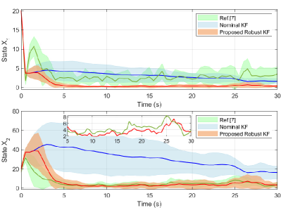
Figure 1: DT robust filter: Mean and standard deviation of the absolute error with initial condition $x_{0}=[20\ 20]^{T}$, for Case II.

TABLE I: Comparison of error in Discrete time filters.

Filter Algorithm		Case I	Case II
		Mean  /  SD	Mean  /  SD
Ref.[7]	$x_{1}$	2.7325 / 1.7518	3.4675 / 2.0216
	$x_{2}$	4.3049 / 2.9640	6.0837 / 3.5487
Nominal KF	$x_{1}$	0.4438 / 0.4136	2.4085 / 1.0595
	$x_{2}$	4.4418 / 4.1355	24.0821 / 10.5982
Proposed Robust KF	$x_{1}$	0.3182 / 0.2914	0.5666 / 0.4314
	$x_{2}$	3.1846 / 2.9114	5.6669 / 4.3099

V-B Continuous-Discrete Robust Kalman Filter

The proposed hybrid robust Kalman filter in §IV-B is applied to the example (26) and its performance is compared with the nominal Kalman filter.

$$\dot{\boldsymbol{x}}(t) =\begin{bmatrix}0&-1+\delta\\ 1&-0.5\end{bmatrix}\boldsymbol{x}(t)+\begin{bmatrix}-2\\ 1\end{bmatrix}\boldsymbol{w}(t),$$ (26a)

$$\boldsymbol{y}(t_{k}) =\begin{bmatrix}-100&-100\end{bmatrix}\boldsymbol{x}(t_{k})+\boldsymbol{n}(t_{k}),$$ (26b)

where $\delta$ is uniformly distributed in the interval $[-0.95\ 0.95]$, and the variances of process and measurement noise are $Q=1$ and $R=1$. We use the similar performance metrics discussed in the previous subsection.

The proposed robust Kalman filter is 2 times more accurate than the nominal KF in steady state as shown in TABLE II. Moreover, it shows faster convergence than the nominal KF as shown in Fig.2. Again, we note that the computational time required for the proposed filter is comparable to the nominal KF.

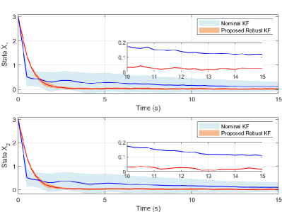
Figure 2: Hybrid robust filter: Mean and standard deviation of the absolute error with initial condition $x_{0}=[3\ 3]^{T}$, for Case II.

TABLE II: Comparison of error in hybrid filters.

Filter Algorithm		Case I	Case II
		Mean  /  SD	Mean  /  SD
Nominal KF	$x_{1}$	0.0223 / 0.0204	0.2052 / 0.1694
	$x_{2}$	0.0195 / 0.0211	0.2038 / 0.1695
Proposed Robust KF	$x_{1}$	0.0155 / 0.0092	0.1833 / 0.0783
	$x_{2}$	0.0137 / 0.0077	0.1822 / 0.0782

VI Conclusion

In this paper, we proposed robust Kalman filter with probabilistic uncertainty in system parameters. Mean and variance of the uncertain system are propagated using conditional probability and the polynomial chaos (PC) expansion framework. The empirical results in this preliminary work show that the proposed approach which exploits the information about probability distribution of the uncertain parameters, demonstrates better performance than the existing frameworks which are designed for the worst case scenarios that occur with the vanishing probability. This serves as a motivation to pursue a theoretical treatment of the performance guarantees for the proposed approach, which is a topic of our ongoing research.

References

- [1] José Claudio Geromel, Maurício C de Oliveira, and Jacques Bernussou. Robust filtering of discrete-time linear systems with parameter dependent lyapunov functions. SIAM Journal on control and optimization, 41(3):700–711, 2002.
- [2] Márcio J Lacerda, Ricardo CLF Oliveira, and Pedro LD Peres. Robust and filter design for uncertain linear systems via lmis and polynomial matrices. Signal Processing, 91(5):1115–1122, 2011.
- [3] Guang-Ren Duan and Hai-Hua Yu. LMIs in control systems: analysis, design and applications. CRC press, 2013.
- [4] Michael Green and David JN Limebeer. Linear robust control. Courier Corporation, 2012.
- [5] F. L. Lewis, L. Xie, and D. Popa. Optimal and robust estimation: with an introduction to stochastic control theory. CRC press, 2017.
- [6] Lihua Xie, Yeng Chai Soh, and Carlos E De Souza. Robust kalman filtering for uncertain discrete-time systems. IEEE Transactions on automatic control, 39(6):1310–1314, 1994.
- [7] X. Zhu, Y. Soh, and L. Xie. Design and analysis of discrete-time robust kalman filters. Automatica, 38(6):1069–1077, 2002.
- [8] Fuwen Yang, Zidong Wang, and YS Hung. Robust kalman filtering for discrete time-varying uncertain systems with multiplicative noises. IEEE Transactions on Automatic Control, 47(7):1179–1183, 2002.
- [9] Wenqiang Liu, Xuemei Wang, and Zili Deng. Robust kalman estimators for systems with mixed uncertainties. Optimal Control Applications and Methods, 39(2):735–756, 2018.
- [10] M. Abolhasani and M. Rahmani. Robust kalman filtering for discrete-time time-varying systems with stochastic and norm-bounded uncertainties. J DYN SYST-T ASME, 140(3), 2018.
- [11] Lihua Xie and Yeng Chai Soh. Robust kalman filtering for uncertain systems. Systems & Control Letters, 22(2):123–129, 1994.
- [12] Peng Shi. Robust kalman filtering for continuous-time systems with discrete-time measurements. IMA Journal of Mathematical Control and Information, 16(3):221–232, 1999.
- [13] Ali H Sayed. A framework for state-space estimation with uncertain models. IEEE T AUTOMAT CONTR, 46(7):998–1013, 2001.
- [14] Mattia Zorzi. Robust kalman filtering under model perturbations. IEEE Transactions on Automatic Control, 62(6):2902–2907, 2016.
- [15] Mattia Zorzi and Bernard C Levy. Robust kalman filtering: Asymptotic analysis of the least favorable model. In 2018 IEEE Conference on Decision and Control (CDC), pages 7124–7129. IEEE, 2018.
- [16] Uri Shaked, Lihua Xie, and Yeng Chai Soh. New approaches to robust minimum variance filter design. IEEE Transactions on Signal Processing, 49(11):2620–2629, 2001.
- [17] R. H. Cameron and W. T. Martin. The Orthogonal Development of Non-Linear Functionals in Series of Fourier-Hermite Functionals. The Annals of Mathematics, 48(2):385–392, 1947.
- [18] Dongbin Xiu and George Em Karniadakis. The Wiener–Askey Polynomial Chaos for Stochastic Differential Equations. SIAM J. Sci. Comput., 24(2):619–644, 2002.
- [19] R. Ghanem and P. Spanos. Polynomial chaos in stochastic finite element. Journal of Applied Mechanics, ASME, 57(1):197–202, 1990.
- [20] R. Ghanem and Pol D. Spanos. Stochastic Finite Elements: A Spectral Approach. Springer-Verlag, New York, NY, 1991.
- [21] Youssef Marzouk and Dongbin Xiu. A Stochastic Collocation Approach to Bayesian Inference in Inverse Problems. Communications in Computational Physics, 6(4):826–847, 2009.
- [22] Lionel Mathelin and M. Yousuff Hussaini. A stochastic collocation algorithm for uncertainty analysis, nasa/cr-2003-212153. Technical report, NASA, 2003.
- [23] R. Walters. Towards stochastic fluid mechanics via polynomial chaos. In 41 st AIAA Aerospace Sciences Meeting & Exhibit, Reno, NV, 2003.
- [24] Serhat Hosder, Robert Walters, and Michael Balch. Efficient sampling for non-intrusive polynomial chaos applications with multiple uncertain input variables. In 48th AIAA/ASME/ ASCE/AHS/ASC Structures, Structural Dynamics, and Materials Conference, page 1939, 2007.
- [25] Paul G Constantine, Michael S Eldred, and Eric T Phipps. Sparse pseudospectral approximation method. Computer Methods in Applied Mechanics and Engineering, 229:1–12, 2012.
- [26] Patrick R Conrad and Youssef M Marzouk. Adaptive smolyak pseudospectral approximations. SIAM Journal on Scientific Computing, 35(6):A2643–A2670, 2013.
- [27] Raktim Bhattacharya. Robust lqr design for systems with probabilistic uncertainty. International Journal of Robust and Nonlinear Control, 29(10):3217–3237, 2019.
- [28] J. Fisher and R. Bhattacharya. Linear quadratic regulation of systems with stochastic parameter uncertainties. Automatica, 45(12):2831–2841, 2009.
- [29] R. Bhattacharya and J. Fisher. Linear receding horizon control with probabilistic system parameters. In 7th IFAC Symposium on Robust Control Design, volume 45, pages 627–632, 2012.
- [30] Parikshit Dutta and Raktim Bhattacharya. Nonlinear Estimation with Polynomial Chaos and Higher Order Moment Updates. In 2010 American Control Conference, Marriott Waterfront, pages 3142–3147, Baltimore, MD, USA, 2010.
- [31] Ivo Babuska, Raúl Tempone, and Georgios E Zouraris. Galerkin finite element approximations of stochastic elliptic partial differential equations. SIAM Journal on Numerical Analysis, 42(2):800–825, 2004.
- [32] Ivo Babuška, Fabio Nobile, and Raul Tempone. A stochastic collocation method for elliptic partial differential equations with random input data. SIAM Journal on Numerical Analysis, 45(3):1005–1034, 2007.
- [33] F. Nobile, R. Tempone, and C. G. Webster. A sparse grid stochastic collocation method for partial differential equations with random input data. SIAM Journal on Numerical Analysis, 46(5):2309–2345, 2008.
- [34] Murray Rosenblatt. Remarks on a multivariate transformation. The annals of mathematical statistics, 23(3):470–472, 1952.
- [35] Armen Der Kiureghian and Pei-Ling Liu. Structural reliability under incomplete probability information. Journal of Engineering Mechanics, 112(1):85–104, 1986.
- [36] George EP Box and David R Cox. An analysis of transformations. Journal of the Royal Statistical Society. Series B (Methodological), pages 211–252, 1964.
- [37] MS Eldred and John Burkardt. Comparison of non-intrusive polynomial chaos and stochastic collocation methods for uncertainty quantification. AIAA paper, 976(2009):1–20, 2009.
- [38] Arthur E. Bryson, Jr. and Yu-Chi Ho. Applied Optimal Control. Hemisphere Publication Corporation, Washington D.C., 1975.