Towards Explainability of Machine Learning Models in Insurance Pricing

Abstract

Machine learning methods have garnered increasing interest among actuaries in recent years. However, their adoption by practitioners has been limited, partly due to the lack of transparency of these methods, as compared to generalized linear models. In this paper, we discuss the need for model interpretability in property & casualty insurance ratemaking, propose a framework for explaining models, and present a case study to illustrate the framework.

1 Introduction

Risk classification for property & casualty (P&C) insurance rating has traditionally been done with one-way, or univariate, analysis techniques. In recent years, many insurers have moved towards using generalized linear models (GLM), a multivariate predictive modeling technique, which addresses many shortcomings of univariate approaches, and is currently considered the gold standard in insurance risk classification. At the same time, machine learning (ML) techniques such as deep neural networks have gained popularity in many industries due to their superior predictive performance over linear models (LeCun, Bengio, and Hinton 2015). In fact, there is a fast growing body of literature on applying ML to P&C reserving (Kuo 2019; Wüthrich 2018; Gabrielli, Richman, and Wüthrich 2019; Gabrielli 2019). However, these ML techniques, often considered to be completely “black box”, have been less successful in gaining adoption in pricing, which is a regulated discipline and requires a certain amount of transparency in models.

If insurers can gain more insight into how ML models behave in risk classification contexts, it would increase their ability to reassure regulators and the public that accepted ratemaking principles are met. Being able to charge more accurate premiums would, in turn, make the risk transfer system more efficient and contribute to the betterment of society. In this paper, we aim to take a step towards liberating actuaries from the confines of linear models in pricing projects, by proposing a framework for explaining ML models for ratemaking that regulators, practitioners, and researchers in actuarial science can build upon.

The rest of this paper is organized as follows: Section 2 provides an overview of P&C ratemaking, Section 3 discusses the importance of interpretation, Section 4 discusses model interpretability in the context of ratemaking and proposes specific tasks for model explanation, Section 5 describes current model interpretation techniques and applies them to the tasks defined in the previous section, and Section 6 concludes.

2 Property and Casualty Ratemaking

2.1 History of Ratemaking

Early classification ratemaking procedures were typically univariate in nature. For example, Lange (1966) notes that (at that time) most major lines of insurance used univariate methods based around the same principle: distributing an overall indication to territorial relativities or classification relativities based on the extent to which they deviated from the average experience.

Bailey and Simon (1960) introduced minimum bias methods, which were expanded throughout the 60s, 70s, and 80s. As computing power developed, minimum bias began to give away to GLMs, with papers such as Brown (1988) and Mildenhall (1999) bridging the gap between the methods.

Arguably, GLMs predate minimum bias procedures by a significant margin. The term was coined by Nelder and Wedderburn (1972), but generalizations of least squares linear regression date back at least to the 1930s. Like minimum bias methods, GLMs did not become mainstream in actuarial science for some time. For example, the syllabus of basic education of the Casualty Actuarial Society (CAS) does not seem to include any mention of GLMs prior to Brown (1988) in the 1990 syllabus. From there, GLMs seem to have received only passing mention until 2006 with the introduction of Anderson et al. (2005) to the syllabus. Beginning in 2016, the CAS introduced Goldburd, Khare, and Tevet (2016) to the syllabus, which offers a comprehensive guide to GLMs.

2.2 Machine Learning in Ratemaking

Paralelling the development of GLM was the development of machine learning algorithms throughout the middle part of the 20th century. Detailed histories of machine learning may be found in sources such as Nilsson (2009) and Wang and Raj (2017). Consistent with GLMs, machine learning was relatively unpopular in actuarial science until the last ten years as computing power has become cheaper and more easily available and as machine learning software packages have obviated the need for developing analyses from scratch each time an analysis is performed. Due to the breadth of machine learning as a field, it is difficult to identify the first time it entered the CAS syllabus; however, cluster analysis (in the form of k-means) seems to have been first included in 2011 with Robertson (2009). More recently, the CAS MAS-I and MAS-II exams introduced in 2018 have included machine learning explicitly.

Within the area of ratemaking, machine learning is still in its infancy. A significant portion of machine learning applications to ratemaking has been in the context of automobile telematics, such as Gao, Meng, and Wuthrich (2018), Gao and Wuthrich (2018), Gao and Wuthrich (2019), Roel, Antonio, and Claeskens (2018), or Wuthrich (2017). Presumably this focus has been a result of the high-dimensionality and complexity of telematics data, making it a field in which the unique abilities of machine learning techniques give a clear advantage over traditional approaches.

Outside of telematics, Yang, Qian, and Zou (2018) use a gradient tree-boosting approach to capture non-linearities that would be a challenge for GLMs. Henckaerts et al. (2018) make use of generalized additive models (GAM) to improve predictions of GLMs. Many researchers, in an apparent effort to demonstrate the range of possibilities and advantages of machine learning, have approached the topic by comparing many different machine learning algorithms within a single study, such as in Dugas et al. (2003), Noll, Salzmann, and Wuthrich (2018), Spedicato, Dutang, and Petrini (2018). These studies make use of such varied techniques as regression trees, boosting machines, support vector machines, and neural networks.

2.3 Ratemaking Process

Regardless of the method employed for determining this risk of various classifications, the actual process of setting rate relativities typically involves some variation of the following steps:

1. Obtain relevant policy-level data

2. Prepare data for analysis

3. Perform analysis on the data, employing desired method(s) to estimate needed rates

4. Select final rates based on rate indications

5. Present rates to the reglator, including explanation of the steps followed to derive the rates

6. Answer questions from regulators regarding the method employed

The focus of this paper is on steps 5 and 6. In many states, rate filings that exceed certain thresholds for magnitude of rate changes or filings that make use of new or sophisticated predictive models may be subject to particular regulatory scrutiny. In these cases, it is necessary to be able to explain the results of the modeling process in a way that is understandable without sacrificing statistical rigor.

It should be noted that communicating results is not simply a method of passing regulatory muster. Generating interpretable modeling output is an important - even essential - facet of model checking. Actuaries are bound by relevant standards to be able to exercise appropriate judgment in selecting risk characteristics as part of a risk classification system per Actuarial Standard of Practice 12 (“Risk Classification”). Therefore, the techniques discussed in this paper may be viewed from the lens of providing useful information to regulators, but they should also be considered as part of a thorough vetting of any rating model.

Although the focus of this paper is on communication to regulators, it should be said that selecting final rates based on indications (step 4 in the list above) may pose a unique challenge for black-box models. This, too, provides strong motivation for techniques that could add to the modeler’s - or any stakeholder’s - understanding of the model, such as the relative importance of variables or the shapes of response curves. Such techniques could be usefully employed in making decisions about how best to select rates.

Similarly, although the focus of this paper is on communication in a pricing context, the techniques explored in this paper (and many of the concerns discussed) may also be relevant to other contexts, such as claim-level reserving or analytics, or other applications of machine learning to the insurance industry.

3 The Need to See Inside the Black Box

Within the actuarial profession, Actuarial Standard of Practice 41 (“Actuarial Communications”) notes that “…another actuary qualified in the same practice area [should be able to] make an objective appraisal of the reasonableness of the actuary’s work as presented in the actuarial report.” (“Actuarial Standard of Practice No. 41 - Actuarial Communications” 2010) Underlying this requirement is an assumption that the hypothetical other actuary qualified in the same practice area is adequately familiar with the relevant techniques employed. Although the syllabus of basic education is constantly changing, there has at times been an assumption that all techniques and assumptions that have ever been a part of the syllabus of basic education needn’t be explained from first principles in general actuarial communications, and that an actuary practicing in the same field should be able to make an objective appraisal of the results from the methods found in the syllabus. This is notable because, beginning with the introduction of the CAS MAS-I and MAS-II examination in July of 2018, several machine learning models were formally included in the syllabus of basic education. These exams cover a wide range of topics, such as splines, clustering algorithms, decision trees, boosting, and principle components analysis (Casualty Actuarial Society 2018).

Nevertheless, machine learning poses something of a special challenge for ASOP 41 for several reasons:

1. Machine learning models can be very ad hoc compared to traditional statistical models.

2. Because many machine learning models do not assume an underlying probability distribution or stochastic process, they may not admit of standard metrics for model comparison (e.g., it’s not straightforward to calculate an AIC over a neural network).

3. Machine learning methods are often combined into ensembles that may not be easily separated and that may, as a collection, cease to resemble a single standard version of a model.

4. Machine learning models can be “black boxes” insofar as the final form of response curve cannot be easily predicted and may depend heavily on the available data (which may not, in turn, be available to the reviewer).

This last item raises a final interesting issue. GLMs and their ilk are often fitted using one of a handful of standard and well-understood approaches (e.g., maximum likelihood estimation). However, this is not possible in general with machine learning models, as machine learning algorithms often use loss surfaces that are very complex such that it may not be feasible to calculate the global minimum of the surface. Certainly, closed form representations of the loss surfaces are not generally available. For this reason, the training phase of a machine learning model is, in many ways, just as important to one’s understanding as the model form and the data on which the model is fitted. Because the final model result is inseparable from these three components (training method, model form, and data), it is not generally adequate to just know the method employed to make an objective appraisal of the reasonableness of the result.

These issues also pose particular challenges with respect to other standards. For instance, as discussed previously, ASOP 12 requires actuaries to be able to exercise appropriate judgment about risk classification systems. The recent ASOP 56 (“Models”) speaks to more general concerns in all practice areas that might make use of models. ASOP 56 requires the actuary to “make reasonable efforts to confirm that the model structure, data, assumptions, governance and controls, and model testing and output validation are consistent with the intended purpose.” (“Actuarial Standard of Practice No. 56 - Modeling” 2019) All of these efforts may be hampered if it is not possible to peer into the black box of the model.

It should also be noted that these comments only apply within the actuarial profession. Outside of the actuarial profession, communication of results may be more challenging. A 2017 survey conducted by the Casualty Actuarial and Statistical Task Force of the National Association of Insurance Commissioners (NAIC) found that the plurality of responding regulators identified “Filing complexity and/or a lack of resources or expertise” as a key challenge that impedes their ability to review GLMs or other predictive models (National Association of Insurance Commissioners 2017). Given that machine learning algorithms are generally regarded as more complex than GLMs, this implies that the challenge of communicating machine learning model results is significant.

In response to the same survey, 33 state regulators noted that it would be helpful or very helpful for the NAIC to develop information and tools to assist in reviewing rate filings based on GLMs, and 34 noted that it would be helpful to develop similar items to assist in reviewing “Other Advanced Modeling Techniques.” One outgrowth of this need was the development of a white paper, National Association of Insurance Commissioners (2019), on best practices for regulatory review of predictive models. The white paper focuses on review of GLMs, particularly with respect to private passenger automobile and homeowners’ insurance. Some of the guidance offered in this regard is therefore not strictly applicable to the review of machine learning models. For example, as previously noted, p-values are not a concept that translates well to deterministic machine learning algorithms. However, among the guidance applicable to machine learning algorithms are the following:

• Determine the extent to which the model causes premium disruption for individual policyholders and how the insurer will explain the disruption to individual consumers that inquire about it.

• Determine that individual input characteristics to a predictive model are related to the expected loss or expense differences in risk. Each input characteristic should have an intuitive or demonstrable actual relationship to expected loss or expense.

• Determine that individual outputs from a predictive model and their associated selected relativities are not unfairly discriminatory.

The last of these items is an entire topic unto itself. The methods and concepts introduced in this paper are useful for exploring the question of whether rates are appropriately related to risk of loss as defined by the variables used in the model, but there are many other aspects of discrimination-free that are outside the scope of this paper. The methods in this paper may help in understanding the model, which is a necessary precursor to addressing the question of unfair discrimination.

The items in this list are by no means exhaustive, but they pertain to the concept of model interpretability for ratemaking that we develop next.

4 Interpretability in the Ratemaking Context

In this section, we attempt to develop a working definition of interpretability for ratemaking applications. While we will not provide a comprehensive survey of the prolific and fast evolving ML interpretability literature, we draw from it as appropriate in setting the stage for our discussion. Even among researchers in the subject, there is not a consensus on the definition of interpretability; here are a few from frequently cited papers:

• Ability to explain or to present in understandable terms to a human (Doshi-Velez and Kim 2017);

• The degree to which an observer can understand the cause of a decision (Biran and Cotton 2017); and

• A method is interpretable if a user can correctly and efficiently predict the method’s results (Kim, Khanna, and Koyejo 2016).

We motivate our discussion by considering several aspects of interpretability. As we proceed through the points below, we aim to arrive at a more scoped and relevant definition of what it means for a pricing model to be interpretable. In the remainder of this section, we clarify a couple concepts regarding interpretable classes of models and the computational transparency of ML models, outline frameworks for understanding the communication goals of interpretability, then discuss a potential framework for implementing ML interpretability in practice.

4.1 Not All Linear Models are Interpretable

In the actuarial science literature, the GLM is probably the most oft-cited example of an easily interpretable model. Given a set of inputs, we can easily reason about what the output of the model is. As an illustrative example, consider a claim severity model with driver age, sex, and vehicle age as predictors; assuming a log link function and letting $Y$ denote the response, we have

$$\log(E[Y])=\beta_{0}+\beta_{1}\cdot\text{age}$$

$$\quad+\beta_{2}\cdot\text{vehicle\_age}+\beta_{3}\cdot\text{sex}_{\text{male}}.$$ (1)

Here, we can tell, for example, what the model would predict for the expected severity if we were to increase age by a certain amount, all else being equal, because the relationship between the predictor and the response is simply multiplication by the coefficient $\beta_{1}$ and applying the inverse link function.

Another commonly cited example of an interpretable model is a decision tree. An illustrative example is shown in Figure 1. Here, the prediction is arrived at by following a sequence of if-else decisions.

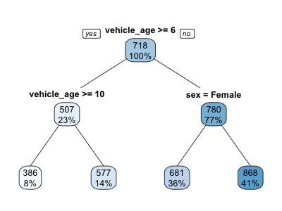
Figure 1: A simple decision tree for loss cost prediction.

Now, it is worth pointing out that, when declaring that GLMs or decision trees are interpretable models, we are implicitly assuming that we are considering only a handful of predictors. In fact, the ease with which we can reason about a model declines as the number of predictors, transformations of them, and interactions increase, as in the following (somewhat pathological) example:

$$\log(E[Y])=\beta_{0}+\beta_{1}\cdot\text{age}+\beta_{2}\cdot\text{vehicle\_age}$$

$$\quad+\beta_{3}\cdot\text{vehicle\_age}^{2}$$

$$\quad+\beta_{4}\cdot\text{age}\cdot\text{vehicle\_age}$$

$$\quad+\beta_{5}\cdot\text{sex}_{\text{male}}+\beta_{6}\cdot\text{sex}_{\text{male}}\cdot\text{age}.$$ (2)

Similarly, one can see that in Figure 2, larger trees are tough to reason about. In other words, even when working within the framework of an “interpretable” class of models, we may still end up with something that many would consider “black box.”

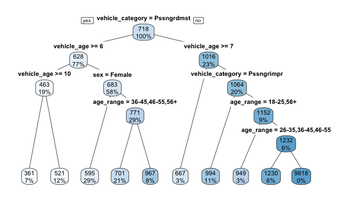
Figure 2: A more complex decision tree. This is still much simpler than typical realistic examples.

4.2 The Machinery is Not a Secret

Another occasional misconception is that we have no visibility into how some ML models compute predictions, which renders them uninterpretable. Outside of proprietary algorithms, all common ML models, including neural networks, gradient boosted trees, and random forests, are well studied and have large bodies of literature documenting their inner workings. As an example, a fitted feedforward neural network is simply a composition of linear transformations followed by nonlinear activation functions. As in Equation 4.1, one can write down the mathematical equation for calculating the prediction given some inputs, but it may be difficult for a human to reason about it. We show later that we can still provide explanations of completely “black box” models, but is important to note that ML model predictions are still governed by mathematical rules, and are deterministic in most cases.

4.3 Explanations are Contextual

Hilton (1990) proposed a framework, later interpreted by Miller (2017) in the context of ML, for understanding model explanations as conversations or social interactions. One consequence of this identification is that explanations need to be relevant to the audience. This framework is consistent with ASOP 41, which formulates a similar requirement in terms of an intended user of the actuarial communication. In developing, filing, and operationalizing a pricing model, one needs to accommodate a variety of stakeholders, each of whom has a different set of questions, assumptions, and technical capacity. First, there are internal stakeholders at the company, which includes management and underwriters. While some of the individuals in this audience may be technical, they are likely less familiar with predictive modeling techniques than the actuaries and data scientists who build the models. Next, we have the regulators, who may have limited resources to review the models, and will focus on a specific list of questions motivated by statute and public policy. Finally, we have potential policyholders, who have an interest (perhaps more so than the other parties) as they are responsible for paying the premiums.

It is interesting to note that the modelers, who are most familiar with the models, tend to be same people designing and communicating the explanations. This poses a challenge that Miller, Howe, and Sonenberg (2017) call “inmates running the asylum”, where the modelers design explanations for themselves rather than the intended audience. For example, they may be interested in technical questions, such as extrapolation behavior, and shape the explanations accordingly, which may be irrelevant to a prospective policyholder.

Another point outlined in Miller’s survey (Miller 2017) is that explanations are contrastive. In other words, people are often interested in not why something happened, but rather why it happened instead of something else. For example, policyholders might not care exactly how their auto premiums are computed, but would like to know why they are being charged more than their coworkers who drive similar vehicles. As an extension, policyholders may want to know what they can change in order to obtain lower premiums.

4.4 Asking and Answering the Right Questions

With the above considerations in mind, we propose a potential framework for interpreting ML models for insurance pricing: the actuarial profession, in collaboration with regulators and representatives of the public, define a set of questions to be answered by explanations accompanying ML models, along with acceptance criteria and examples of successful explanations. In other words, interpretability for our purposes is defined as the ability of a model’s explanations to answer the posed questions.

It should be noted that no ideal set of questions exists that would encompass all potential models. Rather, the actuary must consider what aspects of the model would raise questions from the perspective of the model’s intended users. We propose that relevant stakeholders, by providing example questions and answers, would inherently provide guidance by which actuaries can reasonably anticipate the kinds of specific questions most important to those stakeholders and address them proactively.

These questions should relate to existing guidelines, such as those described in National Association of Insurance Commissioners (2019) and outlined in Section 3, standards of practice, and regulation, and in fact should not be specific only to ML models. By conceptualizing a set of questions, we reduce the burden of both companies and regulators; this is especially important for the latter, who are already resource constrained facing increasing variety of models being filed. This format should also be familiar to actuaries who are accustomed to adhering to specific guidelines in, for example, ASOPs. Like the ASOPs, We envision that these questions and guidelines will be continually updated to reflect feedback obtained and advances in research.

While the realization of a set of such guidelines is an ambitious undertaking beyond the scope of this paper, we present in the next section a sample set of questions and techniques one can leverage to answer them. The goal of these case studies is twofold: to more concretely illustrate the proposed framework, and to expose the actuarial audience to modern ML interpretation techniques.

5 Applying Model Interpretation Techniques

Now that we have established a framework for model interpretation in the form of asking and answering relevant questions, we demonstrate examples of such exchanges via an illustrative case study. Analytically, our starting point is a fitted deep neural network model for predicting loss costs. As the modeling details are of secondary importance, they are available in Appendix A. The questions that we ask of the model are as follows:

1. What are the most important predictors in the model? Put another way, to what extent do the predictors improve the accuracy of the model?

2. How does the predicted loss cost change, on average, as we change an input?

3. For a particular policyholder, how does each characteristic contribute to the loss cost prediction?

The techniques we utilize to answer these questions are permutation variable importance, partial dependence plots, and additive variable attributions, respectively. In our discussion, we adopt the organization of techniques and some notation presented in Molnar and others (2018) and Biecek and Burzykowski (2019), which are comprehensive references on the most established ML interpretation techniques.

5.1 A Simplified View of Interpretation Techniques

Before we dive into the answering questions, we present a brief taxonomy of ML interpretation techniques. Rather than attempting an exhaustive classification, the goal is to orient ourselves among broad categories of techniques, so we can map them to tasks indicated by the questions being asked. For our purposes, model interpretation techniques can be categorized across two dimensions: intrinsic vs. post-hoc and global vs. local.

5.1.1 Intrinsic vs. Post-hoc

Intrinsic model interpretation draws conclusions from the structure of the fitted model and are what we typically associate with “interpretable” classes of models. This is only viable with models with simple structures, such as the sparse linear model and shallow decision tree we see in Section 4.1, where we arrive at explanations by reading off parameter estimates or a few decision rules. For algorithms that produce models with complex structure that do not lend themselves easily to intrinsic exploration, we can appeal to post-hoc techniques. This class of techniques interrogate the model by presenting it with data for scoring and observing the prediction behavior of the model. These techniques are concerned with only the inputs and outputs, and hence are agnostic of the model itself, which means they can also be applied to simple models. Since most useful ML models have a level of complexity beyond the threshold of intrinsic interpretability, we focus on model-agnostic techniques in our case study. As we will see later on, the data that we present to the models are usually some perturbed variations of test data.

5.1.2 Global vs. Local

Along the other dimension, we categorize model interpretations as global, or model-level, and local, or instance-level. The former class provides insights with respect to the model as a whole. Some examples of these eplanations include variable importances and sensitivities, on average, of the predicted response with respect to individual predictors. Note that these methods may be compared to the methods described in (Goldburd, Khare, and Tevet 2016), Chapter 7, which focus on global interpretation of GLMs.

In our case study, questions 1 and 2 are associated with global interpretations. On the other hand, question 3 pertains to an individual prediction, which would fall in the local, or instance-level, category. In addition to individual variable attribution, we can also inquire about what would happen to the current predicted response if we were to perturb specific predictor variables.

5.2 Answering the Questions

Having aligned the questions with the categories of interpretation techniques, we now introduce a selection of appropriate techniques to answer them.

5.2.1 Variable Importance

“What are the most important predictors in the model?”

For linear models and their generalizations, and some ML models, measures of variable importance can be obtained from the fitted model structure. In the case of GLMs, one might observe the magnitudes of the estimated coefficients or $t$-statistics, whereas for random forests, one might use out-of-bag errors (Breiman 2001). For more complex models, such as the neural network in our case study, we need to devise another approach.

We follow the methodology of permutation feature importance as described in Fisher, Rudin, and Dominici (2018), and utilize the notation introduced by Biecek and Burzykowski (2019). The gist of the technique is as follows: to see how important a variable is, we make predictions without it and see how much worse off we are in terms of accuracy. One way to achieve this would be to re-fit the model many times (as many times as the number of variables.) However, this may be intractable with lengthy model training times or large numbers of variables, so a more popular approach is to instead keep the same fitted model but permute the values of each predictor.

More formally, let $y$ denote the vector of responses, $X$ denote the matrix of predictor variables, $\widehat{f}$ denote the fitted model, and $L=\mathcal{L}(\widehat{f}(X),y)$, where $\widehat{f}$ applies to $X$ rowwise, denote the value of the loss function, which is mean squared error in the case of regression. Now, if $\widetilde{X}^{j}$ denotes the predictor matrix where the $j$th variable has been permuted, then we can compute the loss with the permuted dataset as $L^{-j}=\mathcal{L}(\widehat{f}(\widetilde{X}^{j}),y)$. Here, by permuting a variable, we mean that we randomly rearrange the values in the column of data associated with the variable. With this, we define the variable importance $VI^{j}$ as $L^{-j}-L$.

In Figure 3, we show a plot of variable importances. In our particular example, we see that the “make” variable contributes most to the accuracy of the model with “sex” contributing the least. This provides a way for the audience to quickly glance at the most relevant variables, and ask further question as necessary.

Note that these measures do not provide information regarding the directional sensitivity of the predictors on the response. Also, when there are correlated variables, one should be careful about interpretation, as the result may be biased by unrealistic records in the permuted dataset. Another ramification of a group of correlated variables is that their inclusion may cause each to appear less important than if only one is included in the model.

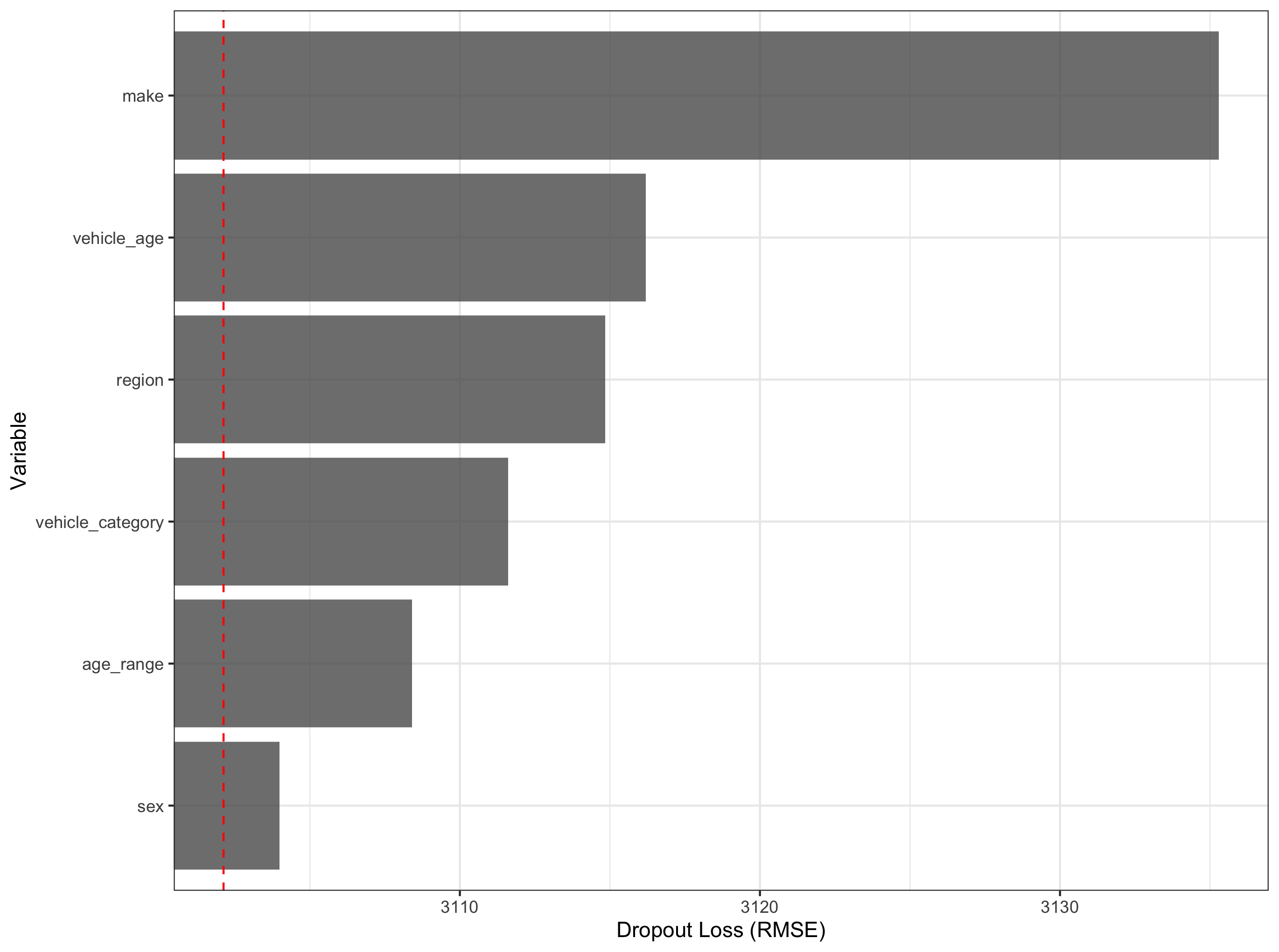
Figure 3: Permutation feature importances for the neural network model.

5.2.2 Partial Dependence Plots

“How does the predicted loss cost change, on average, as we change an input?”

For this question, we again consider first how it would be answered in the GLM setting. When the input predictor in question is continuous, we can answer the question by looking at the estimated coefficient, which provides the change in the response per unit change in the predictor (on the scale of the linear predictor). For non-parametric models and neural networks, where no coefficients are available, we can appeal to partial dependence plots (PDP), first proposed by Friedman (2001) for gradient boosting machines (GBM).

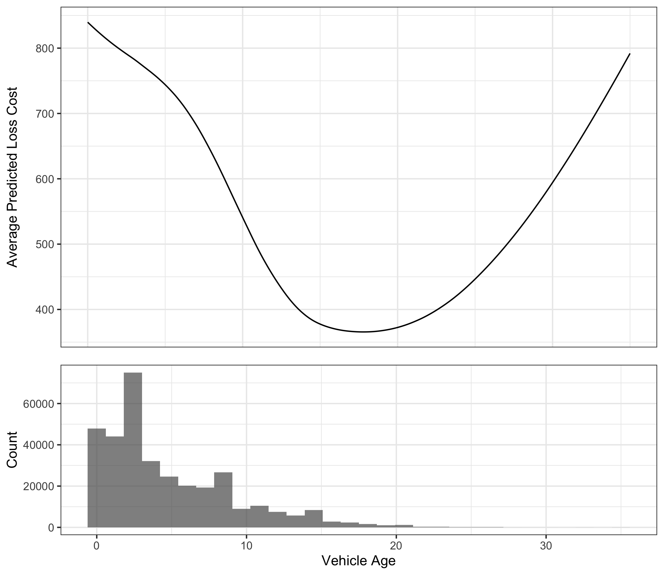
Figure 4: Partial dependence plot for the neural network model.

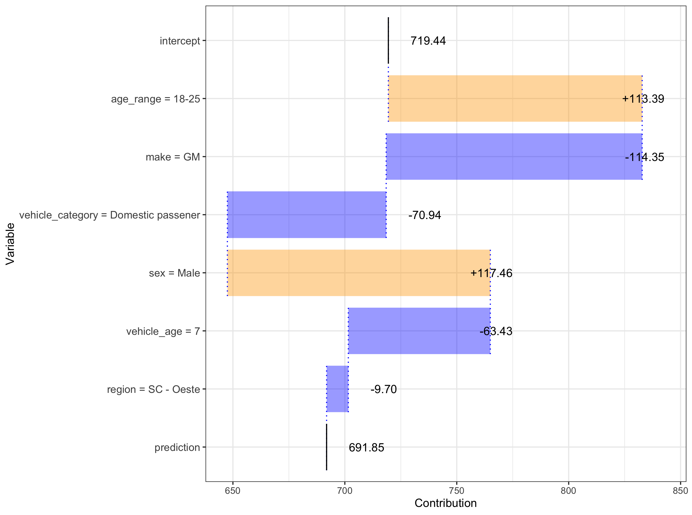
Figure 5: Variable contribution plot for the neural network model.

To describe PDP, we need to introduce some additional notation. Let $x^{j}$ denote the input variable of interest. Then we define the partial dependence function as

$$h(z)=E_{X^{-j}}[\widehat{f}(x|x^{j}=z)],$$ (3)

where the expectation is taken over the distribution of the other predictor variables. In other words, we marginalize them out so we can focus on the relationship between the predicted response and the variable of interest. Empirically, we estimate $h$ by

$$\widehat{h}(z)=\frac{1}{N}\sum_{i=1}^{N}\widehat{f}(x_{i}|x_{i}^{j}=z),$$ (4)

where $N$ is the number of records in the dataset.

In Figure 4, we exhibit the PDP for the “vehicle age” variable. We see that the average predicted loss cost decreases with vehicle age until the latter is around 18. Note that the accompanying histogram shows that the data is quite thin for vehicle age greater than 18, so the apparent upward trend to the right is driven by just a few data points.

This information allows the modeler and stakeholders to consider whether it is reasonable for the anticipated loss cost to follow this shape.

The question posed here is particularly important for regulators, who would like to know whether each variable affects the prediction in the direction that is expected, based on intuition, experience, and existing models. During the model development stage, PDP can also be used as a reasonableness test for candidate models by identifying unexpected relationships for the analyst to investigate.

As with permutation feature importance, one should be careful when interpreting PDP when there are strongly correlated variables. Since we average over the marginal distribution of the rest of the variables, we may take into account unrealistic data (e.g. high vehicle age for a model that is brand new). To address this drawback, alternative visualization techniques have been proposed, such as accumulated local effect (ALE) plots, which take expectations over conditional, rather than marginal, distributions (Apley and Zhu 2016).

5.2.3 Variable Attribution

“For a particular policyholder, how does each characteristic contribute to the loss cost prediction?”

In the previous two examples, we look at model-level explanations; now we move on to one where we investigate one particular prediction instance. As before, we consider how we would approach the question for linear models. For a GLM with a log link common in ratemaking applications, for example, we start with the base rate, then the exponentiated coefficients would have multiplicative effects on the final rate. Similar to the previous examples, for ML models in general we do not have directly interpretable weights. Instead, one way to arrive at variable contributions is calculating the change in the expected model prediction for each predictor, conditioned on other predictors.

Formally, for a fitted model $\widehat{f}$, a given ordering of the variables $X^{1},\dots,X^{p}$, where $p$ is the number of predictor variables, and a specific instance $x_{*}$, we would like to decompose the model prediction $\widehat{f}(x_{*})$ into

$$\widehat{f}(x_{*})=v_{0}+\sum_{j=1}^{p}v(j,x_{*}),$$ (5)

where $v_{0}$ denotes the average model response, and $v(j,x_{*})$ denotes the contribution of the $j$th variable in instance $x_{*}$, defined as

$$v(j,x_{*})=E_{X}[\widehat{f}(X)|X^{1}=x_{*}^{1},\dots,X^{j}=x_{*}^{j}]$$

$$\quad-E_{X}[\widehat{f}(X)|X^{1}=x_{*}^{1},\dots,X^{j-1}=x_{*}^{j-1})].$$ (6)

Hence, the contribution of the $j$th variable to the prediction is the incremental change in the expected model prediction when we set $X^{j}=x_{*}^{j}$ assuming the other variables take their values in $x_{*}$. Note here that this definition implies that the order in which we consider the variables affects the results. Empirically, the expectations in (5.2.3) are calculated by sampling the test dataset.

In Figure 5, we exhibit a waterfall plot of variable contributions. The “intercept” value denotes the average model prediction and represents the $v_{0}$ term in Equation (5). The predicted loss cost for this particular policyholder is slightly less than average; the characteristics that makes this policyholder more risky are the fact that he is a male between the ages of 18 and 25; counteracting the risky driver characteristics are the vehicle properties: it is a GM vehicle built domestically and is seven years old.

Instance-level explanations are useful for investigating specific problematic predictions generated by the model. Regulators and model reviewers may be interested in variable contributions for the safest and riskiest policyholders to see if they conform to intuition. A policyholder with a particularly high premium may wish to find out what of their characteristics contribute to it, and may follow up with a question about how he can lower it, which would require another type of explanation.

As noted earlier, the ordering of variables has an impact on the contributions calculated, especially for models that are non-additive, which could cause inconsistent explanations. There are several approaches to ameliorate this phenomenon, including selecting variables with the largest contributions first, including interactions terms, and averaging over possible orderings. The last of these ideas is implemented by Lundberg and Lee (2017) using Shapley values from cooperative game theory, and is referred to as Shapley additive explanations (SHAP). These approaches are discussed further in Biecek and Burzykowski (2019) and its references. Shapley values were also used in Mango (1998), which has appeared on the CAS syllabus starting in 2004, in the context of determining how to allocate catastrophe risk loads between multiple accounts.

5.3 Other Techniques

In this paper, we demonstrate just a few model-agnostic ML interpretation techniques. These represent a small subset of existing techniques, each of which have additional variations. In the remainder of this section, we point out a few common techniques not covered in our case study.

Individual conditional expectation (ICE) plots disaggregate PDPs into their instance-level components for a more granular view into predictor sensitivities (Goldstein et al. 2015). To accommodate correlated variables in PDP, accumulated local effect (ALE) plots computes expected changes in model response over the conditional, rather than marginal, distribution of the other variables (Apley and Zhu 2016).

Local interpretable model-agnostic explanations (LIME) (Ribeiro, Singh, and Guestrin 2016) builds simple surrogate models using model predictions, with higher training weights given to the point of interest, in effect replacing the complex ML model with an easily interpretable linear regressions or decision trees in neighborhoods of specific points for the purpose of explanation. Taking the concept further, one can also train a global surrogate model across the entire domain of interest.

6 Conclusion

Actuarial standards of practice, most notably ASOP 41, places responsibility on the actuary to clearly communicate actuarial work products, including insurance pricing models. These responsibilities create special challenges for communicating machine learning models, which are often seen “black boxes” due in part to their complexity, nonlinearity, flexible construction, and ad hoc nature.

In this paper, we discuss particular questions of model validation that are of key importance in communicating a model that may present particular difficulty for machine learning models compared to GLMs or traditional pricing models. Specifically,

• How does the model impact individual insurance consumers?

• How are the predictor variables related to expected losses?

We contextualize these questions in terms of different frameworks for defining interpretability. We conceptualize interpretability in terms of the ability of a model (or modeler) to answer a set of idealized questions that would be refined. We then offer potential (families of) model-agnostic techniques for providing answers to these questions.

Much work remains to be done in terms of defining the role of machine learning algorithms in actuarial practice. Lack of interpretability has been a key barrier preventing wider adoption and exploration of these techniques. The methods proposed in this paper could therefore represent important strides in unlocking the potential of machine learning within the insurance industry.

References

Abadi, Martin, Ashish Agarwal, Paul Barham, Eugene Brevdo, Zhifeng Chen, Craig Citro, Greg S. Corrado, et al. 2015. “TensorFlow: Large-Scale Machine Learning on Heterogeneous Systems.” http://tensorflow.org/.

“Actuarial Standard of Practice No. 41 - Actuarial Communications.” 2010. http://www.actuarialstandardsboard.org/wp-content/uploads/2014/02/asop041_120.pdf.

“Actuarial Standard of Practice No. 56 - Modeling.” 2019. http://www.actuarialstandardsboard.org/wp-content/uploads/2020/01/asop056_195.pdf.

Anderson, D., S. Feldblum, C. Modlin, D. Schirmacher, E. Schirmacher, and N. Thandi. 2005. “A Practitioner’s Guide to Generalized Linear Models,” 4–39.

Apley, Daniel W., and Jingyu Zhu. 2016. “Visualizing the Effects of Predictor Variables in Black Box Supervised Learning Models.” http://arxiv.org/abs/1612.08468.

Bailey, Robert A., and LeRoy J. Simon. 1960. “Two Studies in Automobile Insurance Ratemaking.” ASTIN Bulletin 1 (4): 192–217. https://doi.org/10.1017/S0515036100009569.

Biecek, Przemyslaw, and Tomasz Burzykowski. 2019. “Predictive Models: Explore, Explain, and Debug.” https://pbiecek.github.io/PM_VEE/.

Biran, Or, and Courtenay Cotton. 2017. “Explanation and Justification in Machine Learning: A Survey.” In IJCAI-17 Workshop on Explainable AI (XAI), 8:1.

Breiman, Leo. 2001. “Random Forests.” Machine Learning 45 (1): 5–32.

Brown, Robert L. 1988. “Minimum Bias with Generalized Linear Models,” 187–217.

Casualty Actuarial Society. 2018. “Syllabus of Basic Education” 2018. https://www.casact.org/admissions/syllabus/ArchivedSyllabi/2018Syllabus.pdf.

Doshi-Velez, Finale, and Been Kim. 2017. “Towards A Rigorous Science of Interpretable Machine Learning.” arXiv:1702.08608 [Cs, Stat], February. http://arxiv.org/abs/1702.08608.

Dugas, Charles, Y. Bengio, Nicolas Chapados, P. Vincent, G. Denoncourt, and C. Fournier. 2003. “Statistical Learning Algorithms Applied to Automobile Insurance Ratemaking,” December. https://doi.org/10.1142/9789812794246_0004.

Fisher, Aaron, Cynthia Rudin, and Francesca Dominici. 2018. “All Models Are Wrong, but Many Are Useful: Learning a Variable’s Importance by Studying an Entire Class of Prediction Models Simultaneously.” arXiv:1801.01489 [Stat], January. http://arxiv.org/abs/1801.01489.

Friedman, Jerome H. 2001. “Greedy Function Approximation: A Gradient Boosting Machine.” Annals of Statistics, 1189–1232.

Gabrielli, Andrea. 2019. “A Neural Network Boosted Double over-Dispersed Poisson Claims Reserving Model.” SSRN Scholarly Paper ID 3365517. Rochester, NY: Social Science Research Network.

Gabrielli, Andrea, Ronald Richman, and Mario V. Wüthrich. 2019. “Neural Network Embedding of the over-Dispersed Poisson Reserving Model.” Scandinavian Actuarial Journal, 1–29.

Gao, Guangyuan, Shengwang Meng, and Mario V. Wuthrich. 2018. “Claims Frequency Modeling Using Telematics Car Driving Data.” Scandinavian Actuarial Journal.

Gao, Guangyuan, and Mario Wuthrich. 2019. “Convolutional Neural Network Classification of Telematics Car Driving Data.” Risks 7 (January): 6. https://doi.org/10.3390/risks7010006.

Gao, Guangyuan, and Mario V. Wuthrich. 2018. “Feature Extraction from Telematics Car Driving Heatmaps.” European Actuarial Journal 8 (2): 383–406.

Goldburd, Mark, Anand Khare, and Dan Tevet. 2016. “Generalized Linear Models for Insurance Rating.” Casualty Actuarial Society, CAS Monographs Series, no. 5.

Goldstein, Alex, Adam Kapelner, Justin Bleich, and Emil Pitkin. 2015. “Peeking Inside the Black Box: Visualizing Statistical Learning with Plots of Individual Conditional Expectation.” Journal of Computational and Graphical Statistics 24 (1): 44–65.

Henckaerts, Roel, Katrien Antonio, Maxime Clijsters, and Roel Verbelen. 2018. “A Data Driven Binning Strategy for the Construction of Insurance Tariff Classes.” Scandinavian Actuarial Journal 2018 (8): 681–705.

Hilton, Denis J. 1990. “Conversational Processes and Causal Explanation.” Psychological Bulletin 107 (1): 65.

Kim, Been, Rajiv Khanna, and Oluwasanmi O. Koyejo. 2016. “Examples Are Not Enough, Learn to Criticize! Criticism for Interpretability.” In Advances in Neural Information Processing Systems, 2280–8.

Kuo, Kevin. 2019. “DeepTriangle: A Deep Learning Approach to Loss Reserving.” Risks 7 (3): 97.

Lange, Jeffrey T. 1966. “General Liability Insurance Ratemaking.” Proceedings of the Casualty Actuarial Society LIII: 26–53.

LeCun, Yann, Yoshua Bengio, and Geoffrey Hinton. 2015. “Deep Learning.” Nature 521 (7553): 436.

Lundberg, Scott M, and Su-In Lee. 2017. “A Unified Approach to Interpreting Model Predictions.” In Advances in Neural Information Processing Systems 30, edited by I. Guyon, U. V. Luxburg, S. Bengio, H. Wallach, R. Fergus, S. Vishwanathan, and R. Garnett, 4765–74. Curran Associates, Inc. http://papers.nips.cc/paper/7062-a-unified-approach-to-interpreting-model-predictions.pdf.

Mango, Donald F. 1998. “An Application of Game Theory: Property Catastrophe Risk Load.” In Proceedings of the Casualty Actuarial Society, LXXXV:157–86.

Mildenhall, Stephen J. 1999. “A Systematic Relationship Between Minimum Bias and Generalized Linear Models.” Proceedings of the Casualty Actuarial Society LXXXVI: 393–487.

Miller, Tim. 2017. “Explanation in Artificial Intelligence: Insights from the Social Sciences.” arXiv:1706.07269 [Cs], June. http://arxiv.org/abs/1706.07269.

Miller, Tim, Piers Howe, and Liz Sonenberg. 2017. “Explainable AI: Beware of Inmates Running the Asylum or: How I Learnt to Stop Worrying and Love the Social and Behavioural Sciences.” arXiv Preprint arXiv:1712.00547.

Molnar, Christoph, and others. 2018. “Interpretable Machine Learning: A Guide for Making Black Box Models Explainable.” E-Book At< Https://Christophm. Github. Io/Interpretable-Ml-Book/>, Version Dated 10.

National Association of Insurance Commissioners. 2017. “2017 Proceedings of the National Association of Insurance Commissioners.”

———. 2019. “Regulatory Review of Predictive Models 10/15/19 Exposure Draft.” https://content.naic.org/sites/default/files/inline-files/Predictive%20Model%20White%20Paper%20Exposed%2010-15-19.docx.

Nelder, J. A., and R. W. M. Wedderburn. 1972. “Generalized Linear Models.” Journal of the Royal Statistical Society, Series a (general), 135 (3): 370–84.

Nilsson, Nils J. 2009. The Quest for Artificial Intelligence. Cambridge University Press.

Noll, Alexander, Robert Salzmann, and Mario Wuthrich. 2018. “Case Study: French Motor Third-Party Liability Claims.” SSRN Electronic Journal.

R Core Team. 2019. R: A Language and Environment for Statistical Computing. Vienna, Austria: R Foundation for Statistical Computing. https://www.R-project.org/.

Ribeiro, Marco Tulio, Sameer Singh, and Carlos Guestrin. 2016. “Why Should I Trust You?: Explaining the Predictions of Any Classifier.” In Proceedings of the 22nd Acm Sigkdd International Conference on Knowledge Discovery and Data Mining, 1135–44. ACM.

Robertson, J. P. 2009. “NCCI’s 2007 Hazard Group Mapping.” Variance 3 (2): 194–213.

Roel, Verbelen, Katrien Antonio, and Gerda Claeskens. 2018. “Unraveling the Predictive Power of Telematics Data in Car Insurance Pricing.” Royal Statistical Society.

Spedicato, Giorgio, Christophe Dutang, and Leonardo Petrini. 2018. “Machine Learning Methods to Perform Pricing Optimization: A Comparison with Standard Generalized Linear Models.” Variance 12 (1).

Wang, Haohan, and Bhiksha Raj. 2017. “On the Origin of Deep Learning.” arXiv:1702.07800v4 [cs.LG].

Wuthrich, Mario V. 2017. “Covariate Selection from Telematics Car Driving Data.” European Actuarial Journal 7 (1): 89–108.

Wüthrich, Mario V. 2018. “Machine Learning in Individual Claims Reserving.” Scandinavian Actuarial Journal 2018 (6): 465–80.

Yang, Yi, Wei Qian, and Hui Zou. 2018. “Insurance Premium Prediction via Gradient Tree-Boosted Tweedie Compound Poisson Models.” Journal of Business and Economic Statistics 36 (3): 456–70.

Appendix

Table 1: Input variables and their transformations.

Variable	Type	Transformation
Age range	Categorical	One-hot encode
Sex	Categorical	One-hot encode
Vehicle category	Categorical	One-hot encode
Make	Categorical	Embed in $\mathbb{R}^{2}$
Vehicle age	Numeric	Center and scale
Region	Categorical	Embed in $\mathbb{R}^{2}$

Appendix A Model Development

In this appendix, we describe the ML model and the data used to train it. Note that, for our paper, the ultimate goal of the modeling procedure is to develop something that can produce predictions. As a result, we do not follow standard practices for tuning and validation. However, for the sake of completeness and reproducibility, we include an overview of the process here. Implementation is done using the R (R Core Team 2019) interface to TensorFlow (Abadi et al. 2015). The model explanation visualizations utilize the implemention by Biecek and Burzykowski (2019), and the code to reproduce them are available on GitHub.

A.1 Data

We use data from the AUTOSEG (“Automobile Statistics System”) of Brazil’s Superintendence of Private Insurance (SUSEP). The organization maintains policy-characteristics-level data, including claim counts and amounts, for all insured automobiles in Brazil. The data contains variables from policyholder characteristics to losses by peril. We use the records from the first half of 2012, which contains 1,707,651 records. One-fifth of the data is reserved for testing; the remainder is further split into 3/4 of analysis and 1/4 into assessment for determining early stopping.

A.2 Model

Table 1 shows the input variables to our model and their associated transformations. For “make” and “region”, we map each level to a point in $\mathbb{R}^{2}$ through embedding layers. The model predicts expected loss cost for all perils combined. The architecture is a feedforward neural network with two hidden layers with 64 units each. The activations for the hidden layers are ReLU while for the output layer it is softplus. Exposures for each record are used as sample weights during training. We fit the model via ADAM with an initial learning rate of 0.1, a mini-batch size of 10,000, and trigger early stopping when the mean squared error on the asssessment set does not improve for five epochs.