On Gaussian curvatures and singularities of Gauss maps of cuspidal edges

Abstract.

We show relation between sign of Gaussian curvature of cuspidal edge and geometric invariants through types of singularities of Gauss map. Moreover, we define and characterize positivity/negativity of cusps of Gauss maps by geometric invariants of cuspidal edges, and show relation between sign of cusps and of the Gaussian curvature.

1. Introduction

Let $f\colon\Sigma\to\bm{R}^{3}$ be a $C^{\infty}$ map, where $\bm{R}^{3}$ is the Euclidean $3$-space and $\Sigma$ is a domain of $\bm{R}^{2}$. Then a point $p\in\Sigma$ is said to be a singular point of $f$ if $\operatorname{rank}df_{p}<2$ holds. We denote by $S(f)=\{q\in\Sigma\ |\ \operatorname{rank}df_{q}<2\}$ the set of singular points of $f$. A singular point $p\in S(f)$ of $f$ is a cuspidal edge if there exist local diffeomorphisms $\varphi\colon\Sigma\to\bm{R}^{2}$ on the source and $\Phi\colon\bm{R}^{3}\to\bm{R}^{3}$ on the target such that $\Phi\circ f\circ\varphi^{-1}(u,v)=(u,v^{2},v^{3})$, where $u,v$ are coordinates of $\bm{R}^{2}$, namely, $f$ is $\mathcal{A}$-equivalent to the germ $(u,v)\mapsto(u,v^{2},v^{3})$ at $\bm{0}$. (In general, two map germs $f,g\colon(\bm{R}^{n},\bm{0})\to(\bm{R}^{m},\bm{0})$ are $\mathcal{A}$-equivalent if there exist diffeomorphism germs $\varphi\colon(\bm{R}^{n},\bm{0})\to(\bm{R}^{n},\bm{0})$ on the source and $\Phi\colon(\bm{R}^{m},\bm{0})\to(\bm{R}^{m},\bm{0})$ on the target such that $\Phi\circ f\circ\varphi^{-1}=g$ holds.)

If $f$ at $p$ is a cuspidal edge, then $\operatorname{rank}df_{p}=1$ holds, that is, $p$ is a $($co$)$rank one singularity of $f$. It is known that a cuspidal edge is a fundamental singularity of a front in $3$-space (see [2, 14]). Here, a $C^{\infty}$ map $f\colon\Sigma\to\bm{R}^{3}$ is said to be a front if there exists a $C^{\infty}$ map $\nu\colon\Sigma\to S^{2}$ such that

• $\left\langle{df_{q}(X)},{\nu(q)}\right\rangle=0$ for any $q\in\Sigma$ and $X\in T_{q}\bm{R}^{2}$ (orthogonality condition),

• $(f,\nu)\colon\Sigma\to\bm{R}^{3}\times S^{2}$ gives an immersion (immersion condition),

where $S^{2}$ is the unit sphere in $\bm{R}^{3}$ and $\left\langle{\cdot},{\cdot}\right\rangle$ is the canonical inner product of $\bm{R}^{3}$. We call $\nu$ the Gauss map of $f$. By definition, fronts admit certain singularities and the Gauss map even at singular points, and hence they might be considered as a generalization of immersions. There are several studies of surfaces with singularities such as fronts (or frontals which satisfy the above orthogonality condition) from the differential geometric viewpoint (cf. [5, 7, 9, 10, 11, 12, 13, 15, 16, 17, 18, 19, 20, 21, 22, 28, 24, 29, 31, 30, 32, 34, 36, 35, 37]).

We assume that $f$ at $p$ is a cuspidal edge in the following. Then there exist a neighborhood $U$ of $p$ and a regular $C^{\infty}$ curve $\gamma=\gamma(t)\colon(-\varepsilon,\varepsilon)\to U$ with $\gamma(0)=p$ such that $\operatorname{Im}(\gamma)=S(f)\cap U$, where $\operatorname{Im}(\gamma)$ is the image of $\gamma$. We remark that $\gamma$ consists of corank one singularities of $f$. Since $\operatorname{rank}df_{p}=1$, there exists a non-zero vector field $\eta$ on $U$ such that $df_{q}(\eta_{q})=\bm{0}$ for any $q\in S(f)\cap U$. We call $\gamma$ and $\eta$ a singular curve and a null vector field, respectively (cf. [18, 29, 30]).

We set two functions $\lambda,\Lambda\colon U\to\bm{R}$ on $U$ by

(1.1) $$\lambda(u,v)=\det(f_{u},f_{v},\nu)(u,v),\quad\Lambda(u,v)=\det(\nu_{u},\nu_{v},\nu)(u,v)$$

for some coordinates $(u,v)$ on $U$, where $(\ )_{u}=\partial/\partial u$ and $(\ )_{v}=\partial/\partial v$. We call $\lambda$ and $\Lambda$ the signed area density function of $f$ and the discriminant function of $\nu$, respectively (cf. [29, 30]). By definition, $S(f)=\lambda^{-1}(0)$ holds, in particular $\lambda(\gamma(t))=0$. The following useful criterion for a cuspidal edge using $\eta$ and $\lambda$ is known ([18, 30]).

Fact 1.1.

Let $f\colon\Sigma\to\bm{R}^{3}$ be a front and $p\in S(f)$ a corank one singular point of $f$. Then $p$ is a cuspidal edge of $f$ if and only if $\eta\lambda(p)\neq 0$, where $\eta\lambda$ is a directional derivative of $\lambda$ in the direction $\eta$.

We remark that useful criteria for other corank one singularities of fronts and frontals are known (cf. [5, 10, 15, 16, 18, 30]).

Using $\lambda$ and $\Lambda$, the Gaussian curvature $K$ of $f$ is given as $K=\Lambda/\lambda$ on $U\setminus S(f)$ by the Weingarten formula. In general, $K$ is unbounded near $S(f)$ since $\lambda=0$ on $S(f)$. However, using a geometric invariants $\kappa_{\nu}$ called the limiting normal curvature ([21, 29]), the following assertion holds.

Fact 1.2 ([21, 30, 32]).

The Gaussian curvature $K$ is bounded near a cuspidal edge $p\in S(f)\cap U$ if and only if $\kappa_{\nu}$ vanishes along $\gamma$ $($see Figure 1$)$.

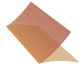
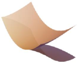
Figure 1. Cuspidal edges with vanishing $\kappa_{\nu}$ (left) and non-vanishing $\kappa_{\nu}$ (right).

On the other hand, the mean curvature $H$ of a front diverges near a corank one singular point ([20, 21, 29]). We note that if the Gaussian curvature $K$ of a front $f$ is bounded near a cuspidal edge $p$, $\Lambda(\gamma(t))=0$ holds, where $\gamma$ is a singular curve of $f$ through $p$ and $\Lambda$ is the function as in (1.1). This implies that $\operatorname{Im}(\gamma)$ is a subset of the singular set $S(\nu)=\Lambda^{-1}(0)$ of $\nu$. Thus the Gauss map $\nu$ has singularities in such cases. It is known that a fold and a cusp naturally appear as singularities of the Gauss map (cf. [3, 4, 38]). If $\nu$ at $p$ is a fold or a cusp, then there exists a $C^{\infty}$ regular curve $\sigma(\tau)$ ($\tau<|\delta|$) such that $\sigma$ parametrizes $S(\nu)$ near $p$ in general (see [14, 38]). We call $\sigma$ a parabolic curve of $f$, and such singular points are called non-degenerate singular points of $\nu$.

In the case that the Gaussian curvature $K$ is bounded, the following assertion about shapes of a cuspidal edge is known.

Fact 1.3 ([29, Theorem 3.1]).

Let $f\colon\Sigma\to\bm{R}^{3}$ be a front with a cuspidal edge $p$. Suppose that the Gaussian curvature $K$ of $f$ is bounded sufficiently small neighborhood $U$ of $p$. If $K$ is positive $($resp. non-negative$)$ on $U$, then the singular curvature $\kappa_{s}$ is negative $($resp. non-positive$)$ at $p$ $($see Figure 2$)$.

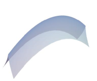
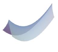
Figure 2. Cuspidal edges with positive $\kappa_{s}$ (left) and negative $\kappa_{s}$ (right).

Here the singular curvature $\kappa_{s}$ is an intrinsic invariant of a cuspidal edge ([9, 11, 21, 29]). This statement tells us that if $K$ is positive and bounded, then a cuspidal edge is curved concavely. We should mention that the inverse of statement as in Fact 1.3 is not true in general (cf. [29]). Thus it is natural to ask the following question: When does the inverse statement as in Fact 1.3 hold?

In this paper, we shall give an answer to this question. More precisely, we show the following.

Theorem A.

Let $f\colon\Sigma\to\bm{R}^{3}$ be a front with a cuspidal edge $p$ and $\nu$ its Gauss map. Suppose that the Gaussian curvature $K$ of $f$ is bounded on a sufficiently small neighborhood $U$ of $p$. When $p$ is a non-degenerate singular point of $\nu$ but not a fold, then $K$ is positive $($resp. negative$\/)$ on $U$ if and only if $\kappa_{s}$ is negative $($resp. positive$\/)$ at $p$.

We next focus on the singular locus $\check{\nu}=\nu\circ\sigma$ of the Gauss map $\nu$, where $\sigma$ is a parabolic curve. The singular locus of a fold is a regular spherical curve and of a cusp is a spherical curve with an ordinary cusp singularity which is $\mathcal{A}$-equivalent to $t\mapsto(t^{2},t^{3})$. For the case of a cusp singularity of the Gauss map, one can define the cuspidal curvature $\mu^{\nu}$ for $\check{\nu}$ ([31, 33]). Using the cuspidal curvature $\mu^{\nu}$, we can define positivity and negativity for a cusp singularity (cf. (4.1) and Definition 4.1). If $K$ is non-zero bounded near a cuspidal edge, then one can take $\sigma(t)$ as $\sigma(t)=\gamma(\pm t)$ near a cuspidal edge (see [32]). In particular, we shall show the following.

Theorem B.

Let $f\colon\Sigma\to\bm{R}^{3}$ be a front, $\nu\colon\Sigma\to S^{2}$ the Gauss map of $f$, $p\in\Sigma$ a cuspidal edge of $f$ and $\gamma(t)$ $(\/t<|\varepsilon|\/)$ the singular curve of $f$ passing through $p(=\gamma(0))$. Take an orientation of $\gamma$ so that the left-hand side of $\gamma$ is $\lambda>0$ on a neighborhood $U(\subset\Sigma)$ of $p$, where $\lambda$ is the signed area density function of $f$ as in (1.1). Suppose that the Gaussian curvature $K$ of $f$ is non-zero bounded on $U$ and $\nu$ has a cusp at $p$. Then $p$ is a positive $($resp. negative$)$ cusp of the singular locus $\check{\nu}=\nu\circ\sigma$ of $\nu$ if and only if $\kappa_{s}$ is positive $($resp. negative$)$ at $p$ when we take the parabolic curve $\sigma(t)$ through $p=\sigma(0)$ as $\sigma(t)=\gamma(t)$.

2. Geometric properties of cuspidal edges

Let $f\colon\Sigma\to\bm{R}^{3}$ be a front with a cuspidal edge at $p\in\Sigma$, where $\Sigma$ is a domain of $\bm{R}^{2}$. Then one can take the following local coordinate system.

Definition 2.1 ([18, 30, 21]).

A local coordinate system $(U;u,v)$ centered at a cuspidal edge $p$ is adapted if it is compatible with respect to the orientation of $\Sigma$ and the following conditions hold:

• the $u$-axis gives a singular curve, that is, $\gamma(u)=(u,0)$ on $U$,

• $\eta=\partial_{v}$ is a null vector field,

• there are no singular points other than the $u$-axis.

Moreover, we call a local coordinate system $(U;u,v)$ a special adapted if it is an adapted coordinate system and the pair $\{f_{u},f_{vv},\nu\}$ is an orthonormal frame along the $u$-axis.

In what follows, we fix an adapted coordinate system $(U;u,v)$ centered at a cuspidal edge $p$ of a front $f$ in $\bm{R}^{3}$. On this local coordinate system, we set the following invariants along the $u$-axis:

(2.1) $$\begin{aligned} \kappa_{s}&=\operatorname{sgn}(\lambda_{v})\dfrac{\det(f_{u},f_{uu},\nu)}{|f_{u}|^{3}},\quad\kappa_{\nu}=\dfrac{\left\langle{f_{uu}},{\nu}\right\rangle}{|f_{u}|^{2}},\quad\kappa_{c}=\dfrac{|f_{u}|^{3/2}\det(f_{u},f_{vv},f_{vvv})}{|f_{u}\times f_{vv}|^{5/2}},\\ \kappa_{t}&=\dfrac{\det(f_{u},f_{vv},f_{uvv})}{|f_{u}\times f_{vv}|^{2}}-\dfrac{\left\langle{f_{u}},{f_{vv}}\right\rangle\det(f_{u},f_{vv},f_{uu})}{|f_{u}|^{2}|f_{u}\times f_{vv}|^{2}}.\end{aligned}$$

These invariants $\kappa_{s}$, $\kappa_{\nu}$, $\kappa_{c}$ and $\kappa_{t}$ are called the singular curvature ([29]), the limiting normal curvature ([29]) and the cuspidal curvature ([21]), the cuspidal torsion ([19]), respectively. We note that $\kappa_{c}$ does not vanish along the $u$-axis when all singular points consist of cuspidal edges ([21, Proposition 3.11]). For $\kappa_{t}$, the following assertion is known.

Fact 2.2 ([17, 36]).

Let $f\colon\Sigma\to\bm{R}^{3}$ be a front with a cuspidal edge $p$ and $\gamma$ a singular curve passing through $p$. Then the singular locus $\hat{\gamma}=f\circ\gamma$ $($or the singular curve $\gamma\/)$ is a line of curvature of $f$ if and only if $\kappa_{t}$ vanishes identically along the singular curve $\gamma$.

For other geometric properties of these invariants, see [9, 12, 11, 21, 19, 29, 17, 36, 34, 35] for example.

On the other hand, we can take a $C^{\infty}$ map $h\colon U\to\bm{R}^{3}\setminus\{\bm{0}\}$ satisfying $f_{v}=vh$ because $f_{v}(u,0)=\bm{0}$ and $\eta\lambda(u,0)=\lambda_{v}(u,0)=\det(f_{u},f_{vv},\nu)(u,0)\neq 0$. Thus $\{f_{u},h,\nu\}$ forms a frame. Using these maps, we define the following functions on $U$: $\widetilde{E}=|f_{u}|^{2}$, $\widetilde{F}=\left\langle{f_{u}},{h}\right\rangle$, $\widetilde{G}=|h|^{2}$, $\widetilde{L}=-\left\langle{f_{u}},{\nu_{u}}\right\rangle$, $\widetilde{M}=-\left\langle{h},{\nu_{u}}\right\rangle$ and $\widetilde{N}=-\left\langle{h},{\nu_{v}}\right\rangle$, where $|\cdot|=\sqrt{\left\langle{\cdot},{\cdot}\right\rangle}$. If we take a special adapted coordinate system $(u,v)$, then invariants as in (2.1) can be written as

(2.2) $$\kappa_{s}=-\dfrac{\widetilde{E}_{vv}}{2},\quad\kappa_{\nu}=\widetilde{L},\quad\kappa_{c}=2{\widetilde{N}},\quad\kappa_{t}=\widetilde{M}$$

along the $u$-axis (see [9, Proposition 1.8], [11, Lemma 3.4] and [36, Lemma 2.7]).

Lemma 2.3.

Take a special adapted coordinate system $(U;u,v)$ centered at a cuspidal edge $p$. Then the differentials $\nu_{u}$ and $\nu_{v}$ of the Gauss map $\nu$ can be expressed as

(2.3) $$\nu_{u}=-\kappa_{\nu}f_{u}-\kappa_{t}h,\quad\nu_{v}=-\dfrac{\kappa_{c}}{2}h$$

along the $u$-axis.

Proof.

By [34, Lemma 2.1], it holds that

$$\nu_{u}=\frac{\widetilde{F}\widetilde{M}-\widetilde{G}\widetilde{L}}{\widetilde{E}\widetilde{G}-\widetilde{F}^{2}}f_{u}+\frac{\widetilde{F}\widetilde{L}-\widetilde{E}\widetilde{M}}{\widetilde{E}\widetilde{G}-\widetilde{F}^{2}}h,\ \nu_{v}=\frac{\widetilde{F}\widetilde{N}-v\widetilde{G}\widetilde{M}}{\widetilde{E}\widetilde{G}-\widetilde{F}^{2}}f_{u}+\frac{v\widetilde{F}\widetilde{M}-\widetilde{E}\widetilde{N}}{\widetilde{E}\widetilde{G}-\widetilde{F}^{2}}h.$$

Since $\widetilde{E}(u,0)=\widetilde{G}(u,0)=1$, $\widetilde{F}(u,0)=0$ and (2.2) hold, we have the assertion. ∎

We now recall principal curvatures. Let $f$ be a front with cuspidal edge $p$. Take an adapted coordinate system $(U;u,v)$ around $p$. Then we set functions $\kappa_{j}\colon U\setminus\{v=0\}\to\bm{R}$ ($j=1,2$) as

$$\kappa_{1}=H+\sqrt{H^{2}-K},\quad\kappa_{2}=H-\sqrt{H^{2}-K},$$

where $K$ and $H$ are the Gaussian and the mean curvature defined on $U\setminus\{v=0\}$. These functions are principal curvatures of $f$ since $\kappa_{1}\kappa_{2}=K$ and $2H=\kappa_{1}+\kappa_{2}$ hold. It is known that one of $\kappa_{j}$ ($j=1,2$) can be extended as a bounded $C^{\infty}$ function on $U$, say $\kappa$, and another, write $\tilde{\kappa}$, diverges near the $u$-axis ([22, 34, 36]). Moreover, $\kappa=\kappa_{\nu}$ holds along the $u$-axis, and $\hat{\kappa}:=\lambda\tilde{\kappa}$ is a bounded $C^{\infty}$ function on $U$ and proportional to $\kappa_{c}$ on the $u$-axis (cf. [36, Theorem 3.1 and Remark 3.2]). In particular, it holds that

(2.4) $$\hat{\kappa}(p)=\dfrac{\kappa_{c}(p)}{2}$$

at a cuspidal edge $p$ when we take a special adapted coordinate system $(U;u,v)$ around $p$ (see [36, Remark 3.2] and (2.2)).

3. Singularities of Gauss maps and the Gaussian curvature

We consider the Gauss map $\nu$ of a front $f\colon\Sigma\to\bm{R}^{3}$ with a cuspidal edge $p$. Let $(U;u,v)$ be an adapted coordinate system around $p$. Then $\kappa$ and $\tilde{\kappa}$ denote the bounded $C^{\infty}$ principal curvature and the unbounded principal curvature on $U$, respectively. Let $\Lambda\colon U\to\bm{R}$ be the discriminant function of $\nu$ as in (1.1). Then the set of singular points of $\nu$ is $S(\nu)=\{q\in U\ |\ \Lambda(q)=0\}$. By the Weingarten formula (cf. [34, Lemma 2.1]), we have

$$\Lambda(u,v)=\kappa(u,v)\hat{\kappa}(u,v)=\lambda(u,v)K(u,v)=\hat{K}(u,v),$$

where $\lambda$ is the signed area density function of $f$ as in (1.1) and $\hat{\kappa}=\lambda\tilde{\kappa}$. Since $\hat{\kappa}(p)\neq 0$, $\Lambda(p)=0$ if and only if $\kappa(p)=\kappa_{\nu}(p)=0$ ([21, 37]). Thus we may assume that $S(\nu)=\{q\in U\ |\ \kappa(q)=0\}$ holds locally. By Fact 1.2, if the Gaussian curvature $K$ is bounded near $p$, then the $u$-axis is also a set of singular points of $\nu$. We say that a singular point $q\in S(\nu)$ of $\nu$ is non-degenerate if $(\partial_{u}\kappa(q),\partial_{v}\kappa(q))\neq(0,0)$, where $\partial_{u}\kappa=\partial\kappa/\partial u$ and $\partial_{v}\kappa=\partial\kappa/\partial v$. Otherwise, we say a degenerate singular point of $\nu$. If $p$ is a non-degenerate singular point of $\nu$, then it follows from the implicit function theorem that there exist a neighborhood $V$ of $p$ and a regular curve $\sigma=\sigma(\tau)\colon(-\delta,\delta)\to V$ ($\delta>0$) such that $\sigma(0)=p$ and $\Lambda(\sigma(\tau))=0$ on $V$ (cf. [3, 4, 14, 27, 38]). We call the curve $\sigma$ the parabolic curve of $f$ or the singular curve of $\nu$.

Lemma 3.1 (cf. [37, Lemma 3.5]).

Let $f\colon\Sigma\to\bm{R}^{3}$ be a front with a cuspidal edge $p$ and $\nu$ the Gauss map of $f$. Suppose that $p$ is also a singular point of $\nu$. Then $p$ is a non-degenerate singular point of $\nu$ if and only if $\kappa_{\nu}^{\prime}(p)\neq 0$ or $4\kappa_{t}(p)^{2}+\kappa_{s}(p)\kappa_{c}(p)^{2}\neq 0$ holds.

Proof.

Let us take a special adapted coordinate system $(U;u,v)$ centered at $p$. Let $\kappa$ be the bounded $C^{\infty}$ principal curvature of $f$ on $U$. Then $\partial_{u}\kappa(p)=\kappa_{\nu}^{\prime}(p)$ holds since $\kappa(u,0)=\kappa_{\nu}(u)$. On the other hand, we have

(3.1) $$\partial_{v}\kappa(p)=-\dfrac{4\kappa_{t}(p)^{2}+\kappa_{s}(p)\kappa_{c}(p)^{2}}{2\kappa_{c}(p)}\neq 0$$

(see [35, Proposition 2.8]). Thus the assertion holds. ∎

Proposition 3.2.

Let $f\colon\Sigma\to\bm{R}^{3}$ be a front with a cuspidal edge $p$. Suppose that the Gaussian curvature $K$ is bounded on a neighborhood $U$ of $p$. Then $p$ is a non-degenerate singular point of the Gauss map $\nu$ if and only if $K$ takes non-zero value near $p$.

Proof.

Let $(U;u,v)$ be a special adapted coordinate system around $p$. Suppose that $K$ is bounded on $U$. Then by Fact 1.2, $\kappa(u,0)=\kappa_{\nu}(u)=0$. Thus there exists a function $\psi\colon U\to\bm{R}$ such that $\kappa(u,v)=v\psi(u,v)$ by the division lemma ([8]), and hence $\psi(p)=\partial_{v}\kappa(p)$. The Gaussian curvature $K$ is given as

$$K=\kappa\tilde{\kappa}=\dfrac{\kappa\hat{\kappa}}{\lambda}=\dfrac{\psi\hat{\kappa}}{\det(f_{u},h,\nu)}$$

on $U$, where $\hat{\kappa}=\lambda\tilde{\kappa}$ and $\lambda=v\det(f_{u},h,\nu)$. Since $\psi(p)=\partial_{v}\kappa(p)$ (see (3.1)), $2\hat{\kappa}(p)=\kappa_{c}(p)$ (see (2.4)) and $\det(f_{u},h,\nu)(p)=1$, we have

(3.2) $$4K(p)=-4\kappa_{t}(p)^{2}-\kappa_{s}(p)\kappa_{c}(p)^{2}$$

(cf. [21, Remark 3.19]). By Lemma 3.1, we get the conclusion. ∎

Remark 3.3.

By this proposition, if the Gaussian curvature $K$ of a front $f$ is bounded at cuapidal edge $p$ and the corresponding Gauss map has a non-degenerate singularity at $p$, then $K$ is automatically non-zero near $p$. Moreover, if $K$ of $f$ is non-zero bounded, $S(f)=S(\nu)$ locally. This means that the parabolic curve $\sigma$ of $f$ satisfies $\sigma(t)=\gamma(\pm t)$ for sufficient small $0<t<|\varepsilon|$.

Remark 3.4.

Proposition 3.2 corresponds to the following statement: a cuspidal edge $p$ of a front $f$ is also a non-degenerate singular point of $\nu$ if and only if $\log|K|$ does not vanish on $U\setminus S(f)$, where $U$ is a neighborhood of $p$. This can be found in [32, Lemma 3.25] in more general situation. Thus Proposition 3.2 might be considered as a rephrasing of [32, Lemma 3.25] in terms of singularities of the Gauss map.

We next consider types of singularities of the Gauss map. It is known that generic singularities of the Gauss map are a fold and a cusp, which are $\mathcal{A}$-equivalent to the germs $(u,v)\mapsto(u,v^{2})$ and $(u,v)\mapsto(u,v^{3}+uv)$ at $\bm{0}$, respectively (cf. [3, 4, 25, 38]). These singularities are non-degenerate singularities of the Gauss map. For singular points of a $C^{\infty}$ map between $2$-dimensional manifolds, see [3, 4, 26, 27, 38].

Fact 3.5 ([37, Proposition 3.12]).

Let $f\colon\Sigma\to\bm{R}^{3}$ be a front with a cuspidal edge $p\in\Sigma$ and $\nu$ its Gauss map. If the Gaussian curvature $K$ of $f$ is non-zero bounded on a sufficiently small neighborhood of $p$, then

• $\nu$ at $p$ is a fold if and only if $\kappa_{t}(p)(4\kappa_{t}(p)^{2}+\kappa_{s}(p)\kappa_{c}(p)^{2})\neq 0$,

• $\nu$ at $p$ is a cusp if and only if $\kappa_{t}(p)=0$, $\kappa_{t}^{\prime}(p)\neq 0$ and $\kappa_{s}(p)\neq 0$.

By Lemma 3.1 and Fact 3.5, we have the following assertion immediately.

Corollary 3.6.

Let $f$ be a front in $\bm{R}^{3}$ with a cuspidal edge $p$. Suppose that the Gaussian curvature $K$ of $f$ is non-zero bounded near $p$. Then $p$ is a non-degenerate singular point other than a fold of $\nu$ if and only if $\kappa_{t}(p)=0$ and $\kappa_{s}(p)\neq 0$.

If $\kappa_{t}$ vanishes identically along the singular curve, namely, if the singular curve is a line of curvature (cf. Fact 2.2), the next assertion holds.

Proposition 3.7.

Let $f\colon\Sigma\to\bm{R}^{3}$ be a front and $p\in\Sigma$ a cuspidal edge. Suppose that the Gaussian curvature $K$ of $f$ is non-zero bounded on a neighborhood $U$ of $p$, and the singular curve $\gamma(t)$ $($in $U)$ through $p$ is a line of curvature of $f$. Then the singular locus $\check{\nu}(t)=\nu(\sigma(t))$ of the Gauss map $\nu$ is a single point in $S^{2}$, where $\sigma(t)=\gamma(\pm t)$.

Proof.

Let us take a special adapted coordinate system $(U;u,v)$ centered at $p$. Assume that $K$ is non-zero bounded on $U$. Then by Proposition 3.2, $p$ is also a non-degenerate singular point of $\nu$. One may choose the parabolic curve $\sigma$ satisfying $\sigma(u)=\gamma(u)$. We consider the behavior of $\nu\circ\sigma(u)=\nu\circ\gamma(u)=\nu(u,0)$. Since $\kappa_{\nu}=0$, we have $\nu_{u}=-\kappa_{t}(u)h(u,0)$ by (2.3) in Lemma 2.3. Thus $\nu_{u}$ is a zero vector along the $u$-axis by the assumption, and hence $\nu$ is a constant map along the $u$-axis. For the case of $\sigma(u)=\gamma(-u)$, we can show in a similar way. ∎

This says that the singular locus $\nu\circ\gamma$ of the Gauss map $\nu$ is a single point if $K$ is non-zero bounded near a cuspidal edge $p$ and $\gamma$ is a line of curvature (see Remark 3.3). In particular, if a surface of revolution has a cuspidal edge and non-zero bounded Gaussian curvature, the image of its Gauss map degenerates to a point.

Example 3.8.

Let $f\colon(-2\pi,2\pi)\times(0,2\pi)\ni(u,v)\mapsto f(u,v)\in\bm{R}^{3}$ be a map given by

$$f(u,v)=((2+\cos{u})\cos{v},(2+\cos{u})\sin{v},u-\sin{u}).$$

This is a cycloid of revolution whose singularities are cuspidal edges. By direct calculations, one can see that $S(f)=\{u=0\}$, $\eta=-\partial_{u}$ and the Gaussian curvature $K$ is negative bounded. Actually, $K=-1/4(2+\cos{u})<0$ holds. Moreover, $\kappa_{s}>0$ and $\kappa_{t}\equiv 0$ hold along the $v$-axis. On the other hand, the Gauss map $\nu$ of $f$ is

$$\nu(u,v)=\left(\sin{\dfrac{u}{2}}\cos{v},\sin{\dfrac{u}{2}}\sin{v},\cos{\dfrac{u}{2}}\right).$$

Note that $S(\nu)=S(f)=\{u=0\}$. By Proposition 3.7, $\nu(S(\nu))$ degenerates to a point. In fact, $\nu(0,v)=(0,0,1)$ holds (see Figure 3).

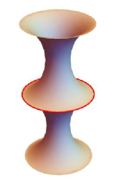
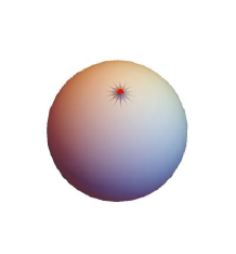
Figure 3. Cycloid of revolution (left) and its Gauss map image (right) of Example 3.8. A curve in the left figure and a point in the right figure which are colored by red are the singular loci of $f$ and $\nu$, respectively.

We remark that a similar statement holds between a flat front in the hyperbolic $3$-space $H^{3}$ and its $\Delta_{1}$-dual flat front in the de Sitter $3$-space $S^{3}_{1}$ (see [28, Corollary 4.3]).

By using above results, we give a proof of Theorem A.

Proof of Theorem A.

Let $(U;u,v)$ be a special adapted coordinate system centered at a cuspidal edge $p$. Since $p$ is a non-degenerate singular point of the Gauss map $\nu$ and the Gaussian curvature $K$ is bounded, $K$ takes non-zero value on $U$. Since $\nu$ at $p$ is not a fold, $\kappa_{t}(p)=0$ and $\kappa_{s}(p)\neq 0$ by Corollary 3.6. Thus $K$ can be written as

$$4K(p)=-\kappa_{s}(p)\kappa_{c}(p)^{2}$$

by (3.2) as in the proof of Proposition 3.2. This completes the proof. ∎

4. Signs of cusps of the Gauss map of a cuspidal edge

We consider the sign of a cusp of the Gauss map of a front with a cuspidal edge. First, we recall the cuspidal curvature for a curve with an ordinary cusp singularity.

Let $S^{2}$ be the standard unit sphere in the Euclidean $3$-space $\bm{R}^{3}$. Note that for any $\bm{x}\in S^{2}$, the tangent plane $T_{\bm{x}}S^{2}$ of $S^{2}$ at $\bm{x}$ can be regarded as $\bm{x}^{\perp}=\{\bm{v}\in\bm{R}^{3}\ |\ \left\langle{\bm{v}},{\bm{x}}\right\rangle=0\}$ of $\bm{x}\in S^{2}\subset\bm{R}^{3}$ by identifying $T_{\bm{x}}\bm{R}^{3}$ with $\bm{R}^{3}$ and considering $T_{\bm{x}}S^{2}\subset\bm{R}^{3}$ as a vector subspace.

Let $c\colon I\to S^{2}$ be a $C^{\infty}$ map, where $I\subset\bm{R}$ is an open interval with a local coordinate $t$. Then we call the curve $c$ a spherical curve. Suppose that a point $t_{0}\in I$ is a singular point of $c$, that is, $(dc/dt)(t_{0})=\dot{c}(t_{0})=\bm{0}$ holds. It is known that $c$ has an ordinary cusp at $t_{0}$ if and only if

$$\det(c,D_{t}\dot{c},D_{t}D_{t}\dot{c})(t_{0})\neq 0,$$

where $D$ is the covariant derivative of $S^{2}$ with $D_{t}=D_{d/dt}$ (cf. [30]).

Let $c\colon I\to S^{2}$ be a spherical curve with an ordinary cusp at $t_{0}\in I$. Then we set

(4.1) $$\mu=\left.\dfrac{\det(c(t),D_{t}\dot{c}(t),D_{t}D_{t}\dot{c}(t))}{|D_{t}\dot{c}(t)|^{5/2}}\right|_{t=t_{0}}.$$

This is a geometric invariant called a cuspidal curvature of $c$ ([31, 33]). The cuspidal curvature does not depend on orientation preserving diffeomorphisms on the source and isometries on the target. We note that the cuspidal curvature $\mu$ can be defined for curves with ordinary cusps in any Riemannian $2$-manifold ([31]).

Let $c\colon I\to S^{2}$ be a spherical curve with an ordinary cusp at $t_{0}\in I$. Then $t_{0}$ is a positive cusp or a zig (resp. a negative cusp or a zag) of $c$ if the cuspidal curvature $\mu$ of $c$ is positive (resp. negative) at $t_{0}$ (cf. [29, 31, 33]) (see Figure 4).

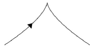
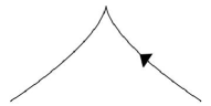
Figure 4. Left: positive cusp (zig). Right: negative cusp (zag). A curve turns right (resp. left) for a cusp if the cuspidal curvature $\mu$ is positive (resp. negative) at that point.

We remark that global studies of zigzag numbers are known (see [1, 6, 29, 30]).

Let $f\colon\Sigma\to\bm{R}^{3}$ be a front with a cuspidal edge $p\in\Sigma$. Assume that the Gauss map $\nu$ of $f$ has a cusp at $p$ and the Gaussian curvature $K$ of $f$ is non-zero bounded on a neighborhood $U$ of $p$. Then there exists a parabolic curve $\sigma(t)$ passing through $p=\sigma(0)$. In this case, the singular locus $\check{\nu}(t):=\nu\circ\sigma(t)(=\nu\circ\gamma(\pm t))$ is a spherical curve with an ordinary cusp singularity at $t=0$. Moreover, we take an orientation of $\gamma(t)$ so that the left-hand side of $\gamma$ is the region of $\lambda>0$ on $U$.

Definition 4.1.

Under the above setting, we call a point $p$ a positive cusp or a zig (resp. a negative cusp or a zag) of $\check{\nu}=\nu\circ\sigma$ if we take $\sigma(t)=\gamma(t)$ and the cuspidal curvature $\mu^{\nu}$ of the singular locus $\check{\nu}$ of $\nu$ is positive (resp. negative) at $p$, where $\gamma$ and $\sigma$ are a singular curve and a parabolic curve of $f$ through $p$, respectively.

Lemma 4.2.

Under the above situation, although we change the Gauss map $\nu$ to $-\nu$ of a front $f$ with cuspidal edge $p$ whose Gaussian curvature is non-zero bounded near $p$, the positivity or negativity of a cusp of the singular locus of the Gauss map does not change.

Proof.

By the definition of the cuspidal curvature (4.1), if we change $\nu$ to $-\nu$, then the cuspidal curvature changes its sign. Moreover, if we change the orientation of $\sigma(=\gamma)$, then the cuspidal curvature also changes the sign by (4.1). On the other hand, if we change $\nu$ to $-\nu$, $\lambda$ changes to $-\lambda$. Thus we need to change the orientation of $\sigma=\gamma$ so that the region of $-\lambda>0$ is the left-hand side of $\gamma$ (cf. Definition 4.1). In this case, the positivity or negativity of a cusp does not change by the above discussion. ∎

Proof of Theorem B.

Let $(U;u,v)$ be a special adapted coordinate system centered at $p$ and assume that the Gaussian curvature $K$ is non-zero bounded on $U$. Then it holds that $\lambda=v\det(f_{u},h,\nu)>0$ on the left-hand side of the $\gamma(u)=(u,0)$, the limiting normal curvature $\kappa_{\nu}$ vanishes identically along the $u$-axis (cf. Fact 1.2) and the $u$-axis is also the set of singular points of $\nu$, that is, $\sigma(u)=(u,0)(=\gamma(u))$ on $U$ (cf. Proposition 3.2 and [32, Lemma 3.25]), where $h\colon U\to\bm{R}^{3}\setminus\{\bm{0}\}$ is a $C^{\infty}$ map satisfying $f_{v}=vh$. Thus the singular locus $\check{\nu}$ of $\nu$ is given as $\check{\nu}(u)=\nu(u,0)$. Moreover, by (2.3) in Lemma 2.3 and the assumption, we have

$$\nu_{u}=-\kappa_{t}h,\quad\nu_{v}=-\dfrac{\kappa_{c}}{2}h$$

along the $u$-axis. Thus $\check{\nu}^{\prime}(u)=-\kappa_{t}(u)h(u,0)$ (${}^{\prime}=d/du$).

To calculate the cuspidal curvature $\mu^{\nu}$ of $\check{\nu}$, we compute the second and the third order differentials of $\check{\nu}$. By direct calculations, we see that

$$\check{\nu}^{\prime\prime}=\dfrac{d^{2}\check{\nu}}{du^{2}}=-\kappa_{t}^{\prime}h-\kappa_{t}h_{u},\quad\check{\nu}^{\prime\prime\prime}=\dfrac{d^{3}\check{\nu}}{du^{3}}=-\kappa_{t}^{\prime\prime}h-2\kappa_{t}^{\prime}h_{u}-\kappa_{t}h_{uu}.$$

Since $\{f_{u},h,\check{\nu}\}$ is an orthonormal frame along the $u$-axis, $h_{u}$ can be written as a linear combination of $f_{u}$, $h$ an $\check{\nu}$. We set

$$h_{u}(u,0)=X_{1}(u)f_{u}(u,0)+X_{2}(u)h(u,0)+X_{3}(u)\check{\nu}(u)$$

along the $u$-axis, where $X_{i}$ $(i=1,2,3)$ are $C^{\infty}$ functions. Since $\left\langle{h},{h}\right\rangle=1$ on the $u$-axis, $X_{2}=0$. Moreover, $X_{3}=\widetilde{M}=\kappa_{t}$ hold because $\left\langle{h},{\check{\nu}}\right\rangle=0$ and $\left\langle{h_{u}},{\check{\nu}}\right\rangle+\left\langle{h},{\check{\nu}^{\prime}}\right\rangle=0$. We consider $X_{1}$. Since $f_{v}=vh$, we see that $h_{u}=f_{uvv}$ on the $u$-axis. On the other hand, $\widetilde{E}_{vv}=\left\langle{f_{u}},{f_{u}}\right\rangle_{vv}=2\left\langle{f_{u}},{f_{uvv}}\right\rangle=2\left\langle{f_{u}},{h_{u}}\right\rangle$ holds along the $u$-axis. Thus by (2.2), we have $X_{1}=-\kappa_{s}$, and hence $h_{u}(u,0)$ is written as

$$h_{u}(u,0)=-\kappa_{s}(u)f_{u}(u,0)+\kappa_{t}(u)\check{\nu}(u).$$

Since $\kappa_{t}(p)=0$ and $\kappa_{t}^{\prime}(p)\neq 0$ by Fact 3.5, we have $\check{\nu}^{\prime}(p)=\bm{0}$,

$$D_{u}\check{\nu}^{\prime}(p)=-\kappa_{t}^{\prime}(p)h(p),\quad D_{u}D_{u}\check{\nu}^{\prime}(p)=-\kappa_{t}^{\prime\prime}(p)h(p)+2\kappa_{t}^{\prime}(p)\kappa_{s}(p)f_{u}(p).$$

Therefore it holds that

$$\det(\check{\nu},D_{u}\check{\nu}^{\prime},D_{u}D_{u}\check{\nu}^{\prime})=2\kappa_{s}(\kappa_{t}^{\prime})^{2},\quad|D_{u}\check{\nu}^{\prime}|^{5/2}=(\kappa_{t}^{\prime})^{2}\sqrt{|\kappa_{t}^{\prime}|}$$

at $p$. Thus the cuspidal curvature $\mu^{\nu}$ of $\check{\nu}$ at $p$ is

$$\mu^{\nu}=\dfrac{2\kappa_{s}(p)}{\sqrt{|\kappa_{t}^{\prime}(p)|}},$$

and hence we have the assertion. If we choose $-\nu$ as the Gauss map of $f$, then we have the same conclusion by Lemma 4.2. ∎

Corollary 4.3.

Under the same assumptions as in Theorem B, if the Gaussian curvature is positive $($resp. negative$)$ near a cuspidal edge $p$, then $p$ is a negative cusp $($resp. a positive cusp$\/)$ of the singular locus of the Gauss map.

Proof.

By Theorems A and B, we have the assertion. ∎

Example 4.4.

Let $f^{\pm}\colon\bm{R}^{2}\to\bm{R}^{3}$ be a $C^{\infty}$ map given by

$$f^{\pm}(u,v)=\left(u,\pm 3u^{2}+\dfrac{v^{2}}{2},\dfrac{v^{3}}{3}+u^{4}\pm u^{2}v^{2}\right).$$

These maps have cuspidal edge at the origin and it follows that $S(f^{\pm})=\{v=0\}$ and $\eta^{\pm}=\partial_{v}$. The Gauss maps $\nu^{\pm}$ of $f^{\pm}$ are

$$\nu^{+}(u,v)=\dfrac{\left(8u^{3}-2uv(v-3),-2u^{2}-v,1\right)}{\sqrt{1+(v+2u^{2})^{2}+(8u^{3}-2uv(v-3))^{2}}},$$

and

$$\nu^{-}(u,v)=\dfrac{\left(8u^{3}-2uv(v-3),2u^{2}-v,1\right)}{\sqrt{1+(v-2u^{2})^{2}+(8u^{3}-2uv(v-3))^{2}}},$$

respectively. In this case, the signed area density function $\lambda^{+}$ (resp. $\lambda^{-}$) for $f^{+}$ (resp. $f^{-}$) is given as $\lambda^{+}=v\varphi$ (resp. $\lambda^{-}=v\psi$) for some positive function $\varphi$ (resp. $\psi$). Thus the left-hand side of $\gamma^{\pm}(u)=(u,0)$ is the region of $\lambda^{\pm}>0$ near the origin.

By a direct computation, we have $\kappa_{\nu}^{\pm}(u)\equiv 0$,

$$\kappa_{s}^{\pm}(u)=\pm\dfrac{6\sqrt{1+24u^{4}+64u^{6}}}{(1+36u^{2}+16u^{6})^{3/2}},\quad\kappa_{t}^{\pm}(u)=\pm\dfrac{4u}{1+4u^{2}+64u^{4}}$$

along the $u$-axis. Thus it follows that $\kappa_{t}^{\pm}(0)=0$, $\kappa_{s}^{\pm}(0)=\pm 6$ and $(\kappa_{t}^{\pm})^{\prime}(0)=\pm 4\neq 0$. This implies that $\nu_{\pm}$ has a cusp at $(0,0)$, and the Gaussian curvature $K^{\pm}$ of $f^{\pm}$ is bounded and $K^{+}<0$ (resp. $K^{-}>0$) near $(0,0)$ (cf. Theorem A). In fact, $K^{\pm}$ are written as

$$K^{+} =\dfrac{-2\left(3+8u^{2}-v\right)}{\left(1+64u^{6}+v^{2}+4u^{4}\left(1+24v-8v^{2}\right)+4u^{2}v\left(1+9v-6v^{2}+v^{3}\right)\right)^{2}},$$

$$K^{-} =\dfrac{2\left(3-8u^{2}-v\right)}{\left(1+64u^{6}+v^{2}+4u^{4}\left(1-24v+8v^{2}\right)+4u^{2}v\left(-1+9v-6v^{2}+v^{3}\right)\right)^{2}},$$

and hence $K^{+}<0$ and $K^{-}>0$ on a sufficiently small neighborhood of the origin.

On the other hand, the singular loci $\check{\nu}^{\pm}(u)=\nu^{\pm}(u,0)$ is

$$\check{\nu}^{+}(u)=\dfrac{\left(8u^{3},-2u^{2},1\right)}{\sqrt{1+4u^{4}+64u^{6}}},\quad\check{\nu}^{-}(u)=\dfrac{\left(8u^{3},2u^{2},1\right)}{\sqrt{1+4u^{4}+64u^{6}}}.$$

These have ordinary cusps at $u=0$, and the cuspidal curvature $\mu_{\pm}^{\nu}$ at $u=0$ are

$$\mu_{\pm}^{\nu}=\pm 6=\dfrac{2\kappa_{s}^{\pm}(0)}{\sqrt{|(\kappa_{t}^{\pm})^{\prime}(0)|}}.$$

Thus $(0,0)$ is a positive (resp. negative) cusp of $\check{\nu}^{+}$ (resp. $\check{\nu}^{-}$)(cf. Corollary 4.3, see Figures 5 and 6).

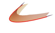
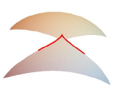
Figure 5. Left: The image of $f^{+}$ given in Example 4.4. The red curve is the image of the curve $\gamma(u)=(u,0)$ by $f^{+}$. Center: The image of the Gauss map $\nu^{+}$. Right: The singular locus $\check{\nu}^{+}$. The dashed curve is the case of $u<0$ and thick curve is of $u>0$. This shows that $\check{\nu}^{+}$ turns right for the cusp.

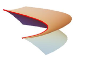
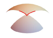
Figure 6. Left: The image of $f^{-}$ given in Example 4.4. The red curve is the image of the curve $\gamma(u)=(u,0)$ by $f^{-}$. Center: The image of the Gauss map $\nu^{-}$. Right: The singular locus $\check{\nu}^{-}$. The dashed curve is the case of $u<0$ and thick curve is of $u>0$. This shows that $\check{\nu}^{-}$ turns left for the cusp.

Acknowledgements.

The author is grateful to Professor Kentaro Saji for fruitful discussions and constant encouragements, and to Professor Osamu Saeki for valuable comments.

References

- [1] V. I. Arnol’d, Topological Invariants of Plane Curves and Caustics, Univ. Lecture Ser. 5, Amer. Math. Soc., Providence, RI, 1994.
- [2] V. I. Arnol’d, S. M. Gusein-Zade and A. N. Varchenko, Singularities of Differentiable Maps. Vol. I., Monographs in Math. 82, Birkhäuser Boston, Inc., Boston, MA, 1985.
- [3] T. Banchoff, T. Gaffney and C. McCrory, Cusps of Gauss Mappings, Research Notes in Math. 55, Pitman, Boston, Mass.-London, 1982.
- [4] D. Bleecker and L. Wilson, Stability of Gauss maps, Illinois J. Math. 22 (1978), 279–289.
- [5] S. Fujimori, K. Saji, M. Umehara and K. Yamada, Singularities of maximal surfaces, Math. Z. 259 (2008), no. 4, 827–848.
- [6] T. Fukunaga and M. Takahashi, Existence and uniqueness for Legendre curves, J. Geom. 104 (2013), no. 2, 297–307.
- [7] T. Fukunaga and M. Takahashi, Framed surfaces in the Euclidean space, Bull. Braz. Math. Soc. (N.S.) 50 (2019), no.1, 37–65.
- [8] M. Golubitsky and V. Guillemin, Stable Mappings and Their Singularities, Grad. Texts in Math. 14, Springer-Verlag, New York-Heidelberg, 1973.
- [9] M. Hasegawa, A. Honda, K. Naokawa, K. Saji, M. Umehara and K. Yamada, Intrinsic properties of surfaces with singularities, Intarnat. J. Math. 26 (2015), no. 4, 1540008, 34 pp.
- [10] A. Honda, M. Koiso and K. Saji, Fold singularities on spacelike CMC surfaces in Lorentz-Minkowski space, Hokkaido Math. J. 47 (2018), no. 2, 245–267.
- [11] A. Honda, K. Naokawa, K. Saji, M. Umehara and K. Yamada, Duality on generalized cuspidal edges preserving singular set images and first fundamental forms, preprint (2019), arXiv:1906.02556.
- [12] A. Honda, K. Naokawa, M. Umehara and K. Yamada, Isometric deformations of wave fronts at non-degenerate signular points, to appear in Hiroshima Math. J., arXiv:1710.02999.
- [13] G. Ishikawa and Y. Machida, Singularities of improper affine spheres and surfaces of constant Gaussian curvature, Internat. J. Math. 17 (2006), no. 3, 269–293.
- [14] S. Izumiya, M. C. Romero Fuster, M. A. S. Ruas and F. Tari, Differential Geometry from a Singularity Theory Viewpoint, World Scientific Publishing Co. Pte. Ltd., Hackensack, NJ, 2016.
- [15] S. Izumiya and K. Saji, The mandala of Legendrian dualities for pseudo-spheres in Lorentz-Minkowski space and ”flat” spacelike surfaces, J. Singul. 2 (2010), 92–127.
- [16] S. Izumiya, K Saji and M. Takahashi, Horospherical flat surfaces in hyperbolic 3-space, J. Math. Soc. Japan 62 (2010), no. 3, 789–849.
- [17] S. Izumiya, K. Saji and N. Takeuchi, Flat surfaces along cuspidal edges, J. Singul. 16 (2017), 73–100.
- [18] M. Kokubu, W. Rossman, K. Saji, M. Umehara and K. Yamada, Singularities of flat fronts in hyperbolic space, Pacific J. Math. 221 (2005), no. 2, 303–351.
- [19] L. F. Martins and K. Saji, Geometric invariants of cuspidal edges, Canad. J. Math. 68 (2016), no. 2, 445–462.
- [20] L. F. Martins, K. Saji and K. Teramoto, Singularities of a surface given by Kenmotsu-type formula in Euclidean three-space, São Paulo J. Math. Sci. 13 (2019), no. 2, 663–677.
- [21] L. F. Martins, K. Saji, M. Umehara and K. Yamada, Behavior of Gaussian curvature and mean curvature near non-degenerate singular points on wave fronts, Geometry and Topology of Manifolds, 247–281, Springer Proc. Math. Stat. 154, Springer, Tokyo, 2016.
- [22] S. Murata and M. Umehara, Flat surfaces with singularities in Euclidean 3-space, J. Differential Geom. 82 (2005), no. 2, 303–351.
- [23] K. Naokawa, M. Umehara and K. Yamada, Isometric deformations of cuspidal edges, Tohoku Math. J. (2) 68 (2016), no. 1, 73–90.
- [24] R. Oset Sinha and F. Tari, On the flat geometry of the cuspidal edge, Osaka J. Math. 55 (2018), no. 3, 393–421.
- [25] I. R. Porteous, Geometric Differentiation. For the Intelligence of Curves and Surfaces, Second edition, Cambridge University Press, Cambridge, 2001.
- [26] J. H. Rieger, Families of maps from the plane to the plane, J. London Math. Soc. (2) 36 (1987), 351–369.
- [27] K. Saji, Criteria for singularities of smooth maps from the plane into the plane and their applications, Hiroshima Math. J. 40 (2010), no. 2, 229–239.
- [28] K. Saji and K. Teramoto, Dualities of differential geometric invariants on cuspidal edges on flat fronts in the hyperbolic space and the de Sitter space, Mediterr. J. Math. 17 (2020), no. 2, Art. 42, 20 pp.
- [29] K. Saji, M. Umehara and K. Yamada, The geometry of fronts, Ann. of Math. (2) 169 (2009), no. 2, 491–529.
- [30] K. Saji, M. Umehara and K. Yamada, singularities of wave fronts, Math. Proc. Cambridge Philos. Soc. 146 (2009), no. 3, 731–746.
- [31] K. Saji, M. Umehara and K. Yamada, The duality between singular points and inflection points on wave fronts, Osaka J. Math. 47 (2010), no. 2, 591–607.
- [32] K. Saji, M. Umehara and K. Yamada, Coherent tangent bundles and Gauss-Bonnet formulas for wave fronts, J. Geom. Anal. 22 (2012), no. 2, 383–409.
- [33] S. Shiba and M. Umehara, The behavior of curvature functions at cusps and inflection points, Differential Geom. Appl. 30 (2012), 285–299.
- [34] K. Teramoto, Parallel and dual surfaces of cuspidal edges, Differential Geom. Appl. 44 (2016), 52–62.
- [35] K. Teramoto, Focal surfaces of wave fronts in the Euclidean 3-space, Glasg. Math. J. 61 (2019), no. 2, 425–440.
- [36] K. Teramoto, Principal curvatures and parallel surfaces of wave fronts, Adv. Geom. 19 (2019), no. 4, 541–554.
- [37] K. Teramoto, Singularities of Gauss maps of wave fronts with non-degenerate singular points, preprint (2018), arXiv:1806.08140.
- [38] H. Whitney, On singularities of mappings of Euclidean spaces. I. Mappings of the plane into the plane, Ann. of Math. (2) 62 (1955), 374–410.