Vortex-Meissner phase transition induced by two-tone-drive-engineered artificial gauge potential in the fermionic ladder constructed by superconducting qubit circuits

Abstract

We propose to periodically modulate the onsite energy via two-tone drives, which can be furthermore used to engineer artificial gauge potential. As an example, we show that the fermionic ladder model penetrated with effective magnetic flux can be constructed by superconducting flux qubits using such two-tone-drive-engineered artificial gauge potential. In this superconducting system, the single-particle ground state can range from vortex phase to Meissner phase due to the competition between the interleg coupling strength and the effective magnetic flux. We also present the method to experimentally measure the chiral currents by the single-particle Rabi oscillations between adjacent qubits. In contrast to previous methods of generating artifical gauge potential, our proposal does not need the aid of auxiliary couplers and in principle remains valid only if the qubit circuit maintains enough anharmonicity. The fermionic ladder model with effective magnetic flux can also be interpreted as one-dimensional spin-orbit-coupled model, which thus lay a foundation towards the realization of quantum spin Hall effect.

LABEL:FirstPage1 LABEL:LastPage#1

I Introduction

Figure 1: (color online). Ladder model constructed by X-shape flux qubits with the gradiometer structure which can cancel out some common flux noise penetrated through the two symmetric loops. The Josephson junctions, flux qubit loop, readout resonator, classical flux bias are colored in gray, red, green, and blue, respectively. The Josephson energy for the big and small Josephson junctions are respectively $E_{J}$ and $\alpha E_{J}$, where $\frac{1}{2}<\alpha<1$ should be satisfied to guarantee the nonlineartiy of the flux qubit and meanwhile, suppress the intercell tunnelling. Meanwhile, the flux qubits are coupled to their nearest neighbours with X-shape mutual inductances that are mostly determined by the nearest edge on the loop. The microwave coplanar waveguide resonator (CPW) is shorted at the terminal near the flux qubit loop such that only inductive coupling is present. The flux qubit loop is designed like a cross such that different coupling terms can be well separately to minimize the crosstalk.

Gauge potential is a core ingredient of the electromagnetic interaction in electrodynamics Jackson1999Book , standard model in particle physics Gaillard1999RMP , and even the topological phenomena in condensed matter physics Hasan2010RMP . However, the behaviours of microscopic particles in gauge potentials are rather difficult to study in natural systems, due to their well-known low controllability. Representatively, for example, strong magnetic field is experimentally challenging to generate for electrons in solid systems. Therefore, engineering effective gauge potential in artificial quantum platform stands a wise option in order to access higher tunability. Superconducting qubit circuits Makhlin2001RMP ; You2005Phys.Today ; Wendin2007LTP ; Clarke2008Nature ; Schoelkopf2008Nature ; Buluta2011RPP ; You2001Nature ; Xiang2013RMP ; Gu2017PR , which inherit the advantages of microwave circuits in flexibility of design, convenience of scaling up, and maturation of controlling technology, have recently won great celebrity in simulating the motions of microscopic particles placed in gauge potentials. In superconducting qubit circuits, photons play the role of carriers, which, in contrast to electrons, will cause no backaction onto the artificial gauge potential due to the charge neutrality.

The engineering of artificial gauge potential (mainly the effective magnetic flux) in superconducting qubit circuits greatly depends on the nonlinearity of Josephson junctions in auxiliary couplers Koch2010PRA ; Nunnenkamp2011NJP ; Marcos2013PRL ; Yang2016PRA ; Roushan2017NP . In this manner, chiral Fock-state transfer Koch2010PRA , multiparticle spectrum modulated by effective magnetic flux in Jaynes-Cummings model Nunnenkamp2011NJP , condensed-matter and high-energy physics phenomena in quantum-link model Marcos2013PRL , and flat band in the Lieb lattice Yang2016PRA have been theoretically studied. In experiment, effective-magnetic-flux-induced chiral currents of single photon and single-photon vacancy have been respectively observed in one-photon and two-photon states Roushan2017NP . By contrast, in cold atom systems, artificial gauge potentials are usually engineered using periodically-modulated onsite energy Aidelsburger2011PRL ; Aidelsburger2013PRL ; Miyake2013PRL ; Atala2014NP . This has motivated the similar proposal of engineering artificial gauge potentials via periodically modulating the Josephson energy of the transmon qubit circuit Alaeian2019PRA , which however maintains valid only in small anharmonicity regime. To remedy this drawback, we propose to modulate the onsite energy of the coupled qubit chain with two-tone drives. This method can in principle be applied to a superconducting qubit circuit with any nonzero anharmonicity, which can thus simulate fermions rather than bosons as in Ref. Alaeian2019PRA . Besides, nonlinearity is known to be a key factor for demonstrating quantum phenomena Wendin2007LTP . Thus, periodically modulating the energy of the qubit circuit with better anharmonicity is significant for exploring nonequilibrium quantum physics.

Meanwhile, thanks to the recent experimental progress in the integration scale of superconducting qubit circuits Barends2014Nature ; Zheng2017PRL ; Song2017PRL ; Gong2019PRL , the quantum simulation research based on superconducting qubit circuits is now advancing from single or several qubits Leak2007Science ; Berger2012PRB ; Berger2013PRA ; Schroer2014PRL ; Zhang2017PRA ; Roushan2014Nature ; Flurin2017PRX ; Ramasesh2017PRL ; Tan2017npj ; Tan2018PRL ; Zhong2016PRL ; Guo2019PRapp towards multiple qubits Roushan2017NP ; Nunnenkamp2011NJP ; Mei2015PRA ; Yang2016PRA ; Tangpanitanon2016PRL ; Gu2017arXiv ; Roushan2017Science ; Xu2018PRL ; Yan2019Science ; Ye2019PRL ; Arute2019Nature . However, most experiments are yet confined to the chain structure (one dimension) currently Roushan2017NP ; Roushan2017Science ; Xu2018PRL ; Yan2019Science , which thus lacks one more dimension to realize the two-dimensional topological phenomena induced by gauge potential, e.g., the quantum Hall effect or quantum spin Hall effect Shen2012Book . Recently, the quasi-two-dimensional ladder model Ye2019PRL , and ture-two-dimensional Sycamore processor Arute2019Nature have both been achieved with the state-of-the-art technology in superconducting quantum circuits, but neither of them involves the research on artificial gauge potential. Therefore, the effect of artificial gauge potential needs to be further explored beyond the one-dimensional system. In particular, the ladder model is almost the simpliest two-dimensional model that implies rich physics, which, for example, can be mapped to the one-dimensional spin-orbit-coupled chain if penetrated by the effective magnetic flux Atala2014NP ; Livi2016PRL .

To make an initial attempt towards two-dimensional quantum simulation with artificial gauge potential, we will design the concrete superconducting qubit circuit that realizes the ladder model penetrated by the effective magnetic flux. We will focus the vortex and Meissner phase transitions induced by the competition of related parameters, such as the coupling strengths and effective magnetic flux. Since the lattice number cannot be achieved so many as the atom number in cold atom systems, we will mainly concentrate on the practical case with finite lattice number. Besides, the method to measure the two phases will also be discussed for the future experimental implementation.

In Sec. II, we introduce the theoretical model that employs two-tone drives to engineer artificial gauge potential in the ladder model constructed by superconducting qubit circuits. In Sec. III, we analyze the Vortex-Meissner phase transition at different parameter regimes. In Sec. IV, we discuss the experimental feasibility to generate the single-particle ground state and measure the vortex-Meissner phase transition. In Sec. V, we summarize the results and make some discussions.

II Two-tone drive induced artificial gauge potential

II.1 Theoretical model

As an example, we consider the ladder model constructed by the X-shape gradiometer flux qubit circuits (see schematic diagram in Fig. 1). The individual flux qubit is manipulated by classical direct current flux bias and alternating current drive (colored in blue), and the states of qubits are dispersively read out through a coplanar waveguide resonator (colored in green) Blais2004PRA ; Lin2014NC ; Yan2016NC ; Wu2018npj . The flux qubits are coupled to their nearest neighbours with mutual inductances that are mostly determined by the nearest edge on the loop. The the flux qubit loop is designed like a cross Barends2013PRL such that different coupling terms can be well separated to minimize the crosstalk. The first (second) row of the qubits is called the left (right) leg of the ladder.

The qubit parameters are assumed to be homogeneous along the leg. Then, the bare Hamiltonian without driving fields can be generally given by

$$\hat{H}_{\text{b}} =\sum_{d=\mathrm{L}}^{\mathrm{R}}\sum_{l}\frac{\hbar}{2}\omega_{d}\hat{\sigma}_{z}^{\left(d,l\right)}$$

$$-\sum_{d=\text{L,R}}\sum_{l}\hbar g_{0}\hat{\sigma}_{-}^{\left(d,l\right)}\hat{\sigma}_{+}^{\left(d,l+1\right)}+\text{H.c.},$$

$$-\sum_{l}\hbar K_{0}\hat{\sigma}_{-}^{\left(\text{L},l\right)}\hat{\sigma}_{+}^{\left(\text{R},l\right)}+\text{H.c..}$$ (1)

Here, according to the homogeneous assumption, all qubits along the $d$ leg have the identical frequency $\omega_{d}$, where $d=\mathrm{L}$ or $d=\mathrm{R}$ is the abbreviation of left or right. The bare intraleg coupling strength on the left (L) or right (R) leg can be given by $g_{d}=M_{d}I_{pd}^{2}/\hbar$ with $d=\mathrm{L,R}$, $M_{d}$ being the mutual inductance between adjacent qubits (e.g., $\sim 10\operatorname{pH}$), $I_{pd}$ the persistent current (e.g., $\sim 0.1\operatorname{\mu A}$), and $\hbar$ the reduced Plank constant. The persistent current and the qubit frequency can be tuned via designing the area ratio $\alpha$ between the small and large junctions Zhu2010APL . Therefore, we can make the qubits on different legs of distinct qubit frequencies. This also leads to $I_{p\text{L}}\neq I_{p\text{R}}$, despite which, however, via careful design of $M_{d}$, we can also make $g_{\text{L}}=g_{\text{R}}=g_{0}$ (e.g., $1\sim 300\operatorname{MHz}\times 2\pi$). Thus, in Eq. (1), the intraleg coupling strengths on both legs are $g_{0}$. Besides, $K_{0}$ denotes the interleg coupling strength, which is determined by the interleg mutual inductance $M$ and also the persistent currents of the flux qubit circuits on both legs, i.e., $K_{0}=MI_{p\mathrm{L}}I_{p\mathrm{R}}$.

To engineer the effective magnetic flux from the bare Hamiltonian $\hat{H}_{\text{b}}$, we will first show that the the qubit frequency can be periodically modulated via the assist of classical driving fields, as will be discussed below.

II.2 Periodical modulation of the qubit frequency

We now demonstrate the periodical modulation of the qubit frequency through two-tone drives. In our treatment, the flux qubit circuit is modelled as an ideal two-level system because of the high anharmonicity Orlandao1999PRB ; Liu2005PRL ; Robertson2006PRB it possesses. In this manner, the individual flux qubit at the $d$ leg and $l$th rung with two-tone drives can be characterized by the Hamiltonian

$$\hat{H}_{d,l}\!=\!\frac{\hbar}{2}\omega_{d}\hat{\sigma}_{z}^{\left(d,l\right)}+\frac{\hbar}{2}\sum_{j=1}^{2}\left[\hat{\sigma}_{+}^{\left(d,l\right)}\Omega_{j}^{\left(d,l\right)}e^{-i\omega_{j}^{\left(d\right)}t}+\mathrm{H.c.}\right],$$ (2)

in the qubit basis, where the $j$th driving field ($j=1,2$) possesses the complex driving strength $\Omega_{j}^{\left(d,l\right)}$ at the frequency $\omega_{j}^{\left(d\right)}$. However, the transmon qubit Koch2007PRA ; Sank2014Thesis has a worse anharmonicity than the flux qubit and thus, the detailed model should include the higher energy levels, e.g., the second excited state (see Appendix. A) .

In Eq. (2), the driving field is determined by the incident current $I_{j}^{\left(d,l\right)}\!\left(t\right)$ through the relation $\operatorname{Re}\{\frac{\hbar}{2}\Omega_{j}^{\left(d,l\right)}e^{-i\omega_{j}^{\left(d\right)}t}\}=-M_{d}I_{pd}I_{j}^{\left(d,l\right)}\!\left(t\right)$. The detunings of the driving frequencies $\omega_{j}^{\left(d\right)}$ from the qubit frequencies $\omega_{d}$ are kept identical for both ladder legs, i.e., $\delta_{j}\equiv\omega_{j}^{\left(d\right)}-\omega_{d}$ despite $d$ taking $\mathrm{L}$ or $\mathrm{R}$. In fact, this can be achieved via tuning the driving frequencies $\omega_{j}^{\left(d\right)}$ for the given qubit frequencies $\omega_{d}$. Besides, we assume $\delta_{1}$ and $\delta_{2}$ are close to each other, i.e., $\left|\delta\right|\ll|\delta_{1}|,|\delta_{2}|$ with $\delta=\delta_{2}-\delta_{1}$. Also, we consider the large-detuning regime $|\Omega_{j}^{\left(d,l\right)}/\delta_{j}|^{2}\ll 1$ and homogeneous (inhomogeneous) driving strengths (phases), i.e., $\Omega_{1}^{\left(d,l\right)}=\Omega_{1}$ and $\Omega_{2}^{\left(d,l\right)}=\Omega_{2}e^{-i\phi_{d,l}}$ with positive $\Omega_{j}$. Then, via the second-order perturbative method, the effective Hamiltonian can be yielded (see Appendix. A) as

$$\hat{H}_{d,l}^{\left(\text{eff}\right)}\!=\!\frac{\hbar}{2}\omega_{d}\hat{\sigma}_{z}^{\left(d,l\right)}\!-\frac{\hbar}{2}\!\left[\omega_{s}\!+\!\Omega\cos(\delta t\!+\!\phi^{\left(d,l\right)})\right]\!\hat{\sigma}_{z}^{\left(d,l\right)},$$ (3)

where $\omega_{s}=\sum_{j=1}^{2}\frac{\Omega_{j}{}^{2}}{2\delta_{j}}$ is the Stark shift and $\Omega=|\frac{\Omega_{1}\Omega_{2}}{\delta_{1}}|$. The phase $\phi^{\left(d,l\right)}$ can be tuned by the driving field at the site $(d,l)$, which will not be specified at present.

In Eq. (3), we find that the qubit frequency is periodically modulated with the strength $\Omega$, the frequency $\delta$, and the phase $\phi^{\left(d,l\right)}$. Under our assumption, the parameters can be typically, $\delta_{1}^{\left(d\right)}/2\pi=1~{}\mathrm{GHz}$, $\delta_{2}^{\left(d\right)}/2\pi=1.1~{}\mathrm{GHz}$, and $\Omega_{1}/2\pi=\Omega_{2}/2\pi=178$ $\mathrm{MHz}$, in which case, the Stark shift $\omega_{s}/2\pi=30.24~{}\mathrm{MHz}$, the modulation strength is $\Omega/2\pi=31.7~{}\mathrm{MHz}$ and the modulation frequency $\delta/2\pi=100~{}\mathrm{MHz}$. The qubit frequency $\omega_{d}/2\pi\$can be about $2~{}\mathrm{GHz}$, which, together with the driving frequencies $\omega_{j}^{\left(d\right)}$, is left to be exactly determined in the following.

Note that one driving field will only arouse transitions between qubit bases [see the individual driving term in Eq. (2)]. That’s why we apply two-tone driving fields to achieve the periodical modulation of the qubit frequency.

We must also mention that the method introduced here is applicable for all qubit circuits, and not merely confined to the flux qubit (see Appendix. A). Its validity does not require a negligibly small anharmonicity of the qubit circuit as that for the transmon circuit in Ref. Alaeian2019PRA . Since nonlinearity is a key factor for demonstrating quantum phenomena Wendin2007LTP , periodically modulating the qubit frequency while maintaining enough anharmonicity can be significant for exploring nonequilibrium quantum physics.

II.3 Engineering effective magnetic flux

Based on the periodical modulation of the qubit frequency in Sec. II.2, we now continue to demonstrate how to engineer the effective magnetic flux. We assume each qubit in Fig. 1 is driven by two-tone fields such that the qubit frequency can be modulated as in Eq. (3). To include the nearest qubit-qubit couplings, the full Hamiltonian can be represented as

$$\hat{H}_{\text{f}}=\hat{H}_{\text{b}}-\sum_{d=\mathrm{L}}^{\mathrm{R}}\sum_{l}\frac{\hbar}{2}\left[\omega_{s}+\Omega\cos(\delta t+\phi^{\left(d,l\right)})\right]\hat{\sigma}_{z}^{\left(d,l\right)}.$$ (4)

Note that $\hat{H}_{\text{b}}$ is the bare Hamiltonian given in Eq. (1), $\omega_{s}$ is the Stark shift, and $\Omega$, $\delta$, and $\phi^{(d,l)}$ are respectively the periodical modulation strength, frequency, and phase of the qubit at $(d,l)$.

To eliminate the time-dependent terms in Eq. (4), we now apply to Eq. (4) a unitary transformation

$$\hat{U}_{d}\left(t\right)={\textstyle\prod\limits_{l}}{\textstyle\prod\limits_{d=\mathrm{L,R}}}\exp\left[i\hat{F}_{l,d}\left(t\right)\right],$$ (5)

where the expression of $\hat{F}_{l,d}\left(t\right)$ is explicitly given by

$$\hat{F}_{l,d}\left(t\right)=\frac{1}{2}\hat{\sigma}_{z}^{\left(d,l\right)}\left[\frac{\Omega}{\delta}\sin\left(\delta t+\phi_{d,l}\right)+\left(\omega_{d}-\omega_{s}\right)t\right].$$ (6)

After that, the assumptions $\phi_{d\text{,}l}=\phi_{d}-\phi l$, $\phi_{\text{L}}=-\phi_{\text{R}}=\phi_{0}$, and $\delta=\omega_{\text{R}}-\omega_{\text{L}}$ are made and the fast-oscillating terms are neglected, thus leading to the following qubit ladder Hamiltonian as

$$\hat{H}_{\text{f}}^{\prime}= -\sum_{d=\text{L}}^{\text{R}}\sum_{l}\hbar g\hat{\sigma}_{-}^{\left(d,l\right)}\hat{\sigma}_{+}^{\left(d,l+1\right)}+\text{H.c.}$$

$$-\sum_{l}\hbar K\hat{\sigma}_{-}^{\left(\text{L},l\right)}\hat{\sigma}_{+}^{\left(\text{R},l\right)}\exp\left(i\phi l\right)+\text{H.c..}$$ (7)

Here, the intraleg coupling strength $g=g_{0}J_{0}\left(\eta_{x}\right)$, and the interleg coupling strength $K=K_{0}J_{1}\left(\eta_{y}\right)$, which are in principle tunable via modifying $\Omega$, since $\eta_{x}=\frac{2\Omega}{\delta}\sin(\frac{\phi}{2})$ and $\eta_{y}=\frac{2\Omega}{\delta}\sin\left(\phi_{0}\right)$ (see Appendix. B for details). The symbol $J_{n}\left(x\right)$ represents the $n$th Bessel function of the first kind.

For the typical parameters given previously, which yields $\Omega/2\pi=31.7\operatorname{MHz}$ and $\delta/2\pi=100\operatorname{MHz}$, we can further set $g_{0}/2\pi=3.5\operatorname{MHz}$, and $K_{0}/2\pi=33\operatorname{MHz}$. Then, the condition $|\eta_{x/y}/2|^{2}\ll 1$ is fulfilled, which makes $g\approx g_{0}$ and $K\approx\frac{\eta_{y}}{2}K_{0}=\frac{\Omega}{\delta}K_{0}\sin\left(\phi_{0}\right)$. In this case, the intraleg coupling strength is fixed at $g_{0}$, but the interleg coupling strength can also be equivalently represented as

$$K\approx 3g\sin\phi_{0}.$$ (8)

This implies that for given $g$, $K$ can be tuned via $\phi_{0}$ in the range $-3g\leq K\leq 3g$ (see Fig. 2), which enables us to study the phase transition by adjusting $K$. The condition $\delta=\omega_{\text{R}}-\omega_{\text{L}}$ can be satisfied with making the qubit frequencies $\omega_{\text{L}}/2\pi=1.9\operatorname{GHz}$ and $\omega_{\text{R}}/2\pi=2\operatorname{GHz}$ such that $\delta/2\pi=100\operatorname{MHz}$. Furthermore, the driving frequencies should be $\omega_{1}^{\left(\text{L}\right)}/2\pi=2.9\operatorname{GHz}$, $\omega_{2}^{\left(\text{L}\right)}/2\pi=3\operatorname{GHz}$, $\omega_{1}^{\left(\text{R}\right)}/2\pi=3\operatorname{GHz}$, and $\omega_{2}^{\left(\text{R}\right)}=3.1\operatorname{GHz}$, since we have assumed $\delta_{1}/2\pi=(\omega_{1}^{\left(d\right)}-\omega_{d})/2\pi=1\operatorname{GHz}$ and $\delta_{2}/2\pi=(\omega_{2}^{\left(d\right)}-\omega_{d})/2\pi=1.1\operatorname{GHz}$.

So far, we have determined nearly all the necessary parameters of the qubit and driving fields, except for the phases in the driving fields $\phi$ and $\phi_{0}$, among which, the former acts as the effective magnetic flux per plaquette, while the latter is used to tune the interleg coupling strength $K$.

II.4 Fermionic ladder in the effective magnetic flux

To transform the qubit ladder into the fermionic ladder, we can make a Jordan-Wigner transformation Mei2013PRB , which is of the form as

$$\hat{\sigma}_{-}^{\left(\text{L},l\right)} =\hat{b}_{\text{L},l}\prod_{l^{\prime}=1}^{l-1}\exp\!(i\pi\hat{b}_{\text{L},l}^{{\dagger}}\hat{b}_{\text{L},l}),$$ (9)

$$\hat{\sigma}_{-}^{\left(\text{R},l\right)} =\hat{b}_{\text{R},l}\prod_{l^{\prime}=1}^{l}\exp(i\pi\hat{b}_{\text{L},l}^{{\dagger}}\hat{b}_{\text{L},l})\!\prod_{l^{\prime}=1}^{l-1}\exp(i\pi\hat{b}_{\text{R},l}^{{\dagger}}\hat{b}_{\text{R},l}).$$ (10)

Here, $\hat{\sigma}_{z}^{\left(d,l\right)}=2\hat{b}_{d,l}^{{\dagger}}\hat{b}_{d,l}-1$, and the fermionic anticommutation relations $\{\hat{b}_{d,l},\hat{b}_{d^{\prime},l^{\prime}}^{{\dagger}}\}=\delta_{dd^{\prime}}\delta_{ll^{\prime}}$ and $\{\hat{b}_{d,l},\hat{b}_{d^{\prime},l^{\prime}}\}=0$ are fulfilled, where $\delta_{dd^{\prime}}$ and $\delta_{ll^{\prime}}$ are Kronecker delta functions. Then, the qubit ladder Hamiltonian $\hat{H}_{\text{f}}^{\prime}$ in Eq. (7) can be transformed into the Hamiltonian of the fermionic ladder, i.e.,

$$\hat{H}_{\text{ld}}= -\sum_{d=\text{L}}^{\text{R}}\sum_{l}\hbar g\hat{b}_{d,l}\hat{b}_{d,l+1}^{{\dagger}}+\text{H.c.}$$

$$-\sum_{l}\hbar K\hat{b}_{\text{L},l}\hat{b}_{\text{R},l}^{{\dagger}}\exp\left(i\phi l\right)+\text{H.c.,}$$ (11)

which describes the motion of “fermionic” particles, governed by the effective magnetic flux $\phi$. We note that the above fermionic ladder model with effective magnetic flux can also be interpreted as one-dimensional spin-orbit-coupled model Atala2014NP ; Livi2016PRL , which may thus inspire the research towards the realization of quantum spin Hall effect Shen2012Book .

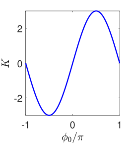
Figure 2: (color online). Tunable interleg coupling strength $K$ plotted versus the phase $\phi_{0}$: $K=3g\sin\phi_{0}$, where, for simplicity, we have set the intraleg coupling strength $g=1$. Here, $\phi_{0}$ is determined by the phases of the driving fields.

III Vortex-Meissner phase transition

III.1 Infinite-length ladder

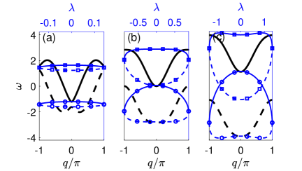
Figure 3: (color online) Single-photon spectrum of the ladder model at the interleg coupling strength $K=$ (a) $0.2$, (b) $\sqrt{2}$, and (c) $2.5$, respectively. Here, the effective magnetic flux $\phi=\frac{\pi}{2}$, and the intraleg coupling strength is set as unity: $g=1$, implying the critical interleg coupling strength $K_{\mathrm{c}}=\sqrt{2}$. The solid (dashed) dark blue curve means $\omega=\omega_{+}$ $(\omega_{-})$, and $z=\exp(iq)$; the solid (dashed) light blue curve marked with “$\square$” means $\omega=\omega_{+}$ $(\omega_{-})$, and $z=\exp(\lambda)$; the solid (dashed) light blue curve marked with “$\circ$” means $\omega=\omega_{+}$ $(\omega_{-})$, and $z=-\exp(\lambda)$.

Now, we seek the energy spectrum of the ladder Hamiltonian $\hat{H}_{\text{ld}}$ in the infinite chain case [see Eq. (11)], i.e., the lattice site (or rung) number $N$ approaches infinity. To do this, we straightforwardly assume that the single-particle eigenstate at the energy $\hbar\omega$ is $\left|\omega\right\rangle=\sum_{d,l}\psi_{d,l}\left|d,l\right\rangle$. Here, the notation $\left|d,l\right\rangle=\hat{b}_{d,l}^{{\dagger}}\left|0\right\rangle$ represents the single-particle state at the site $\left(\mathrm{L},l\right)$ and $\left|0\right\rangle$ is the ground state. Afterwards, we assume the wave function $\psi_{d,l}\equiv\psi_{d,l}\left(z\right)$, and further assume

$$\psi_{\text{L},l}=\psi_{\text{L},0}z^{l}e^{-i\frac{\phi}{2}l}\text{ and }\psi_{\text{R,}l}=\psi_{\text{R,}0}z^{l}e^{i\frac{\phi}{2}l}$$ (12)

before substituting the eigenstate vector $\left|\omega\right\rangle$ into the following secular equation

$$\hat{H}_{\text{ld}}\left|\omega\right\rangle=\hbar\omega\left|\omega\right\rangle.$$ (13)

Then, the dispersion relation can be yielded as a two-band spectrum i.e.,

$$\omega=\omega_{\pm}=-2gz_{\text{p}}^{2}\cos\frac{\phi}{2}\pm\sqrt{K^{2}-4g^{2}z_{\text{m}}^{2}\sin^{2}\frac{\phi}{2}},$$ (14)

where the intermediate parameters $z_{\text{p}}=(z+z^{-1})/2$ and $z_{\text{m}}=(z-z^{-1})/2$. The corresponding wave function at $l=0$ is of the form

$$\psi_{\text{L},0}\!\left(z\right)=\omega+g(ze^{i\frac{\phi}{2}}+z^{-1}e^{-i\frac{\phi}{2}})\text{ and }\psi_{\text{R,}0}\!\left(z\right)=-K,$$ (15)

where a global normalized constant has been discarded.

To guarantee the existence of $\omega$, there can be the following three cases, i.e., (i) $z=\exp\left(iq\right)$, (ii) $z=\exp\left(\lambda\right)$, and (iii) $z=-\exp\left(\lambda\right)$, where $q$ and $\lambda$ must be in the regime $-\pi\leq q\leq\pi$ and $-\ln\Lambda\leq\lambda\leq\ln\Lambda$, where the parameter $\Lambda=K/2g\sin\frac{\phi}{2}+\sqrt{K^{2}/4g^{2}\sin^{2}\frac{\phi}{2}+1}$. Here, the case (i) gives a transmission state, the case (ii) a decay state, and the case (iii) a staggered decay state. In the case (i), the value of $K$ can control the number of the minimums of $\omega_{-}$, for which, there exists a critical interleg coupling strength with the analytical form

$$K_{\text{c}}=2g\tan\frac{\phi}{2}\sin\frac{\phi}{2}.$$ (16)

The relation $K=K_{\text{c}}$ actually yields the vortex-Meissner transition boundary discussed afterwards. In detail, if $K<$ $K_{\text{c}}$, the lower band $\omega_{-}$ has two minimums, while, otherwise, the minimum number is one. This can be clearly found from the dashed black curve in Fig. 3(a)-3(c) for $K$ taking $0.5$, $\sqrt{2}$, and $2.5$, respectively, where we specify $g=1$ and $\phi=\frac{\pi}{2}$ such that $K_{\text{c}}=\sqrt{2}$. As $K$ is increased, the band gap between the two transmission bands $\omega_{+}$ and $\omega_{-}$ will also be broadened. In Fig. 3, where the energy bands $\omega_{\pm}$ for the decay and staggered decay states have also been shown, we also find that a given single-particle energy will always correspond to four degenerate states. This is critical for the existence of the single-particle eigenstates under the open boundary condition, which can in principle be constructed by the linear superposition of these four degenerate states. Only when the decay and staggered decay states are included, one can definitely ensure the equality between the number of the independent coefficients and that of the boundary conditions, considering that there are four terminals of the ladder. However, in the simplest one-dimensional chain, which has only two terminals, the single-particle eigenstates under the open boundary condition is only the superposition of two transmission states, which differs from the quasi-two-dimensonal ladder model this present paper concentrates on.

III.2 Open-boundary ladder with finite qubit number

Now we invstigate the open-boundary condition for the ladder model. In cold atom systems, the ideal open-boundary effect is a hard wall, which is very hard to realize  Atala2014Thesis , and the open-boundary condition is approximately engineered by an external power law potential. However, in superconducting qubit systems, the open-boundary condition is very convenient to realize, since the ladder length is finite in experiment. Suppose the ladder length is $N$, then the fermionic Hamiltonian in Eq. (11) becomes

$$\hat{H}_{\text{ld}}^{\left(N\right)}= -\sum_{l=1}^{N-1}\sum_{d=\text{L}}^{\text{R}}\hbar g\hat{b}_{d,l}\hat{b}_{d,l+1}^{{\dagger}}+\text{H.c.}$$

$$-\sum_{l=1}^{N}\hbar K\hat{b}_{\text{L},l}\hat{b}_{\text{R},l}^{{\dagger}}\exp\left(i\phi l\right)+\text{H.c.,}$$ (17)

where the eigenstates are different from those of the infinite-length ladder, and therefore must be revisited. In Figs. 3(a)-3(c), we find that in infinite-length case, a definite $\omega$ corresponds to four states, which we denote by the characteristic constants $z=z_{1},$ $z_{2},$ $z_{3},$ and $z_{4}$, respectively. In our study, we are only interested in the low-energy states. Thus, the parameters $z_{j}$ can be determined by the relation $\omega=\omega_{-}$ [see Eq. (14)], which yields

$$z_{1,2} \equiv z_{1,2}\left(\omega\right)=\frac{1}{2}(R_{-}\mp\sqrt{R_{-}^{2}-4}),$$ (18)

$$z_{3,4} \equiv z_{3,4}\left(\omega\right)=\frac{1}{2}(R_{+}\mp\sqrt{R_{+}^{2}-4}),$$ (19)

with the compact symbols $R_{\pm}$, determined by $\omega$, represented in the form as

$$R_{\pm}=-\frac{\omega}{g}\cos\frac{\phi}{2}\pm\sqrt{-\frac{\omega^{2}}{g^{2}}\sin^{2}\frac{\phi}{2}+\frac{K^{2}}{g^{2}}+4\sin^{2}\frac{\phi}{2}}.$$ (20)

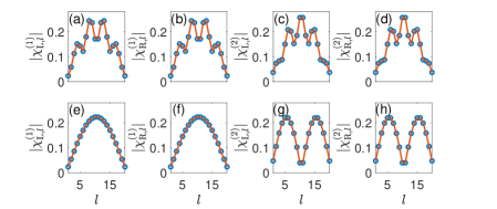
Figure 4: (color online). Probability amplitude $|\chi_{d,l}^{\left(n\right)}|$ for the lowest two states $\chi_{d,l}^{\left(n\right)}$ ($n=1,2$, and $d=$L,R) for the energy $\mu_{n}$ in the open-boundary condition. Here, $n$ denotes the index of the energy level, $d$ the ladder leg, and $l$ the rung index. The “$\circ$” marks the direct numerical diagonalization result, and the solid curve is the fitted result using the expansion equation $\chi_{d,l}^{\left(n\right)}=\sum_{j=1}^{4}A_{j}^{\left(n\right)}\chi_{d,l}^{\left(n,j\right)}$, where $\chi_{d,l}^{\left(n,j\right)}$ is the $j$th transmission or decay state in the infinite-length condition for the energy $\hbar\mu_{n}$. In (a)-(d), the interleg coupling strength $K=0.5$, while in (e)-(h), $K=2.5$. The intraleg coupling strength $g=1$, the effective magnetic flux per plaquette $\phi=\frac{\pi}{2}$ for which $K_{\text{c}}=\sqrt{2}$, and the ladder length $N=20$.

For the open-boundary ladder with finite qubit number, the single-particle eigenstate at the energy $\hbar\mu$ can be assumed as

$$\left|\mu\right\rangle=\sum_{d=\text{L}}^{\text{R}}\sum_{l=1}^{N}\chi_{d,l}\left|d,l\right\rangle.$$ (21)

Here, the eigen wave function $\chi_{d,l}\equiv\chi_{d,l}\!\left(\mu\right)$ must be the linear superposition of the four degenerate states at the energy $\omega=\mu$ of the infinite-length ladder, respectively denoted as $\psi_{d,l}^{\left(j\right)}\equiv\psi_{d,l}\left(z_{j}\left(\mu\right)\right)$ [see Eqs. (12), (18), and (19)], i.e.,

$$\chi_{d,l}=\sum_{j=1}^{4}\!A_{j}\psi_{d,l}^{\left(j\right)}.$$ (22)

Then, by substituting the state vector expansion $\left|\mu\right\rangle$ in Eq. (21) into the secular equation

$$\hat{H}_{\text{ld}}^{\left(N\right)}\left|\mu\right\rangle=\hbar\mu\left|\mu\right\rangle,$$ (23)

where the coefficients $A_{j}$ must be constrained nonzero, the eigen energies can in principle be discretized as $\mu=\hbar\mu_{n}$ ($n=1,2,...,2N$) with $\mu_{n}\leq\mu_{n+1}$ and the corresponding eigenstates can be assumed of the form

$$\left|\mu_{n}\right\rangle=\sum_{d=\text{L}}^{\text{R}}\sum_{l=1}^{N}\chi_{d,l}^{\left(n\right)}\!\left|d,l\right\rangle.$$ (24)

Here, the lowest energy eigenstate $|\mu_{1}\rangle$ is called the single-particle ground state, which is the major state we will study. The eigen wave function $\chi_{d,l}^{\left(n\right)}$ can also be expanded as the linear superposition of $\psi_{d,l}^{\left(n,j\right)}\equiv\psi_{d,l}\left(z_{j}\left(\mu_{n}\right)\right)$, the degenerate states in the infinite-length case, i.e.,

$$\chi_{d,l}^{\left(n\right)}=\sum_{j=1}^{4}A_{j}^{\left(n\right)}\psi_{d,l}^{\left(n,j\right)}.$$ (25)

However, straightforwardly solving Eq. (23) is difficult, since a transcendental equation will be involved. Thus, in this paper, the determination of $A_{j}^{\left(n\right)}$ is achieved by fitting Eq. (25) with the results obtained from direct numerical diagonalization of Eq. (23).

In Fig. 4, the wave functions of the single-particle ground state $\left|\mu_{1}\right\rangle$ and single-particle excited state $\left|\mu_{2}\right\rangle$ ($\mu_{1}<\mu_{2}$) have been shown for $K\$taking $0.5$ [see Fig. 4(a)-4(d)] and $2.5$ [see Fig. 4(e)-4(h)], respectively, where the other parameters are $g=1$, $N=20$, and $\phi=\frac{\pi}{2}$ such that $K_{\text{c}}=\sqrt{2}$. The discrete circles represent the results from the direct numerical diagonalization using Eq. (23), while the solid curves the fitting results using the expansion equation in Eq. (25). Both results can be found to fit each other exactly. Also, the wave functions at $K=2.5>K_{\text{c}}$ appear smoother than those at $K=0.5<K_{\text{c}}$. Besides, when $K=2.5$, $|\chi_{d,l}^{\left(2\right)}|$ exhibits an obvious dip near the middle lattice site, which nevertheless does not occur when $K=0.5$.

Then, we investigate the properties of the single-particle ground state $\chi_{d,l}^{\left(1\right)}$ using the expansion coefficients $A_{j}^{\left(n\right)}$ from fitting. From the discussions in Sec. III.1, we know that if $K\$is less than $K_{\text{c}}$, all the four characteristic constants $z_{j}$ correpsonding to $\omega=\mu_{1}$ are complex numbers on the unit circle, while, if $K$ exceeds $K_{\text{c}}$, $z_{3}$ and $z_{4}$ will become real, which will only contribute to the population at the edges. Due to the effective magnetic flux, a complex characteristic constant $z_{j}=\exp\left(iq_{j}\right)$ corresponds to a plane wave with the quasimomentum $q_{j}-\phi/2$ ($q_{j}+\phi/2$) in the wave function of the L (R) ladder leg [see Eq. (12)].

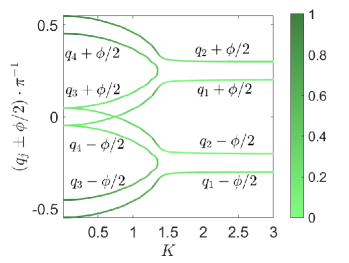
Figure 5: (color online). Quasimomentum $q_{j}\pm\phi/2$ in the single-particle ground state wave function $\chi_{d,l}^{\left(1\right)}$ for different interleg coupling strength $K$. Here, the effective magnetic flux $\phi=\pi/2$, the intraleg coupling strength $g=1$, and the ladder length $N=20$. The color indicates the relative distribution intensity of the wave function on the quasimomentum component. Here, the quasimomentum $q_{j}-\phi/2$ ($q_{j}+\phi/2$) only occurs on the L (R) ladder leg.

In Fig. 5, we have plotted the quasimomentum $q_{j}\mp\phi/2$ versus the interleg coupling strength $K$ with $\phi=\pi/2$ and $N=20$, where the color represents the relative distribution intensity on a particular quasimomentum component [obtained by rescaling $|A_{j}^{\left(1\right)}\psi_{d,0}^{\left(1,j\right)}|$, with $d$ taking L (R) for $q_{j}-\phi/2$ ($q_{j}+\phi/2$)]. We can also see that if $\phi=\pi/2$, and $K$ is less than $K_{\text{c}}$, the particle is more likely to be populated on the L (R) leg, corresponding to the characteristic constant $z_{1,3}$ ($z_{2,4}$). However, if $K$ exceeds $K_{\text{c}}$, only $z_{1}$ and $z_{2}$ remain complex, and the particles corresponding to $z_{1,2}$ are approximately populated uniformly on both legs.

Lastly, we mention that once the single-particle eigenstates $\chi_{d,l}^{\left(n\right)}$ are obtained, one can make the transformation $\hat{b}_{n}^{{\dagger}}=\sum_{d=\text{L}}^{\text{R}}\sum_{l=1}^{N}\chi_{d,l}^{\left(n\right)}\hat{b}_{d,l}^{{\dagger}}$, which can finally transform the Hamiltonian in Eq. (17) into the independent fermionic modes, i.e.,

$$\hat{H}_{\text{ld}}^{\left(N\right)}=\sum_{n=1}^{2N}\hbar\mu_{n}\hat{b}_{n}^{{\dagger}}\hat{b}_{n}.$$ (26)

Here, $\hat{b}_{n}$ and $\hat{b}_{n}^{{\dagger}}$ meet the fermionic anticommutation relations, i.e., $\{\hat{b}_{n},\hat{b}_{n^{\prime}}^{{\dagger}}\}=\delta_{nn^{\prime}}$. Compared with the infinite-length scenario, we note that the eigen energies are discretized, with the eigenstates being the superposition of the ones in the infinite-length scenario.

III.3 Chiral current

The current operator can be derived from the following continuity equation

$$\frac{\text{d}}{\text{d}t}(\hat{b}_{d,l}^{{\dagger}}\hat{b}_{d,l})=\frac{[\hat{b}_{d,l}^{{\dagger}}\hat{b}_{d,l},\hat{H}_{\text{ld}}]}{i\hbar}=\hat{j}_{l-1,l}^{\left(d\right)}+\hat{j}_{l+1,l}^{\left(d\right)}+\hat{j}_{l,\bar{d}d},$$ (27)

where $d,\bar{d}\in\{$L,R$\}$ and $\bar{d}\neq d$. Here, $\hat{j}_{l,l+1}^{\left(d\right)}$ denotes the particle current flowing from the site $l$ to $l+1$ on the $d$ ladder, while $\hat{j}_{l,\bar{d}d}$ the particle current flowing from the $\bar{d}$ ladder to $d$ ladder at the $l$th site. The physical meaning is that the time-varying rate of the particle number at one individual site is determined by the current that flows into it. The resulting current operator can be explicitly represented as

$$\hat{j}_{l,l+1}^{\left(d\right)} =ig(\hat{b}_{d,l+1}^{{\dagger}}\hat{b}_{d,l}-\hat{b}_{d,l}^{{\dagger}}\hat{b}_{d,l+1}),$$ (28)

$$\hat{j}_{l,\text{LR}} =iK(\hat{b}_{\text{R},l}^{{\dagger}}\hat{b}_{\text{L},l}e^{i\phi l}-\hat{b}_{\text{L},l}^{{\dagger}}\hat{b}_{\text{R},l}e^{-i\phi l}).$$ (29)

For the specific single-particle ground state $\left|\mu_{1}\right\rangle=\sum_{d=\text{L}}^{\text{R}}\sum_{l=1}^{N}\chi_{d,l}^{\left(1\right)}\left|d\text{,}l\right\rangle$, the average particle current can be respectively given by

$$j_{l,l+1}^{\left(d\right)}=ig(\chi_{d,l+1}^{\left(1\right)\ast}\chi_{d,l}^{\left(1\right)}-\chi_{d,l+1}^{\left(1\right)}\chi_{d,l}^{\left(1\right)\ast})$$ (30)

which describes the flow from the site $l$ to $l+1$ on the $d$ ladder, and

$$j_{l,\text{LR}}=iK(\chi_{\text{R},l}^{\left(1\right)\ast}\chi_{\text{L},l}^{\left(1\right)}e^{i\phi l}-\chi_{\text{R},l}^{\left(1\right)}\chi_{\text{L},l}^{\left(1\right)\ast}e^{-i\phi l})$$ (31)

which describes the flow from the L to R ladder at the $l$th site.

The presence of the effective magnetic flux will make the system exhibit the property of chirality. In detail, the particle currents on both legs differ from each other. To quantify the difference, we define the chiral particle current as

$$j_{\text{C}}=j_{\text{L}}-j_{\text{R}}.$$ (32)

Here, $j_{d}=(N-1)^{-1}\sum_{l=1}^{N-1}j_{l,l+1}^{\left(d\right)}$ with $d=\mathrm{L,R}$ is the site-averaged current on the particular $d$ leg. In Fig. 6, the chiral current strength is plotted as a function of the flux $\phi$ and interleg coupling strength $K$. The Meissner and vortex phase are separated by a critical boundary, where $K=2g\tan\frac{\phi}{2}\sin\frac{\phi}{2}$ [see Eq. (16)] is fulfilled. This boundary corresponds to the degeneracy transition of the single-particle ground state in the infinite-length case [see Figs. 3(a)-3(c)]. For given $K=\sqrt{2}$, the chiral current first increases as $\phi$ untill reaching its maximum at $\phi_{\text{c}}=\frac{\pi}{2}$ and then goes down towards zero, while, for given $\phi=\frac{\pi}{2}$, the chiral current also first increases as $K$ untill reaching its maximum at $K_{\text{c}}=\sqrt{2}$ but never changes afterwards. The current patterns of the Meissner and vortex phase will be discussed below.

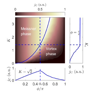
Figure 6: (color online). Chiral current strengths $j_{\text{C}}$ as a function of the effective magnetic flux $\phi$ and the interleg coupling $K$ with $N=20$ sites, $g=1$, and open boundary conditions. The solid curve is the critical boundary separating the Meissner and vortex phase where $K=2g\tan\frac{\phi}{2}\sin\frac{\phi}{2}$ is fulfilled. The right graph shows the chiral current against $K$ at $\phi=\pi/2$, while the bottom shows the chiral current against $\phi$ at $K=\sqrt{2}$. In the right one, the chiral current first increases with $K$ in the vortex phase and then remains unchanged once the critical value $K_{\text{c}}$ is met, which signifies the Meissner phase. In the bottom one, the chiral current first rises with $\phi$ in the Meissner phase until a critical value $\phi_{\text{c}}$ is reached, after which the vortex phase is entered.

III.4 Current patterns in the vortex and Meissner phases

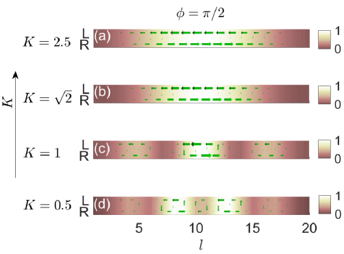
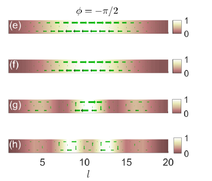
Figure 7: (color online). Current patterns and photon densities for different values of the interleg coupling $K$. Here, the intraleg coupling $g=1$, the flux $\phi=\pi/2$ for the left column and $-\pi/2$ for the right one, the site number $N=20$. The current strength, normalized to the maximum current for each $K$, is denoted by the thickness and length of the arrows. The shade of the color represents the photon density, which is also normalized to its maximum value for each $K$. The flux $\phi=\pm\pi/2$ makes the critical value of the interleg coupling $K_{\text{c}}=\sqrt{2}$, the value that separates the vortex and Meissner phases. In the first row, $K=2.5$, and the currents mainly flow around the edges of the ladder, which, forming one large vortex, is called the Meissner phase. In the second row, $K=\sqrt{2}$, which is the phase transition point, and the current pattern also belongs to Meissner phase. From the third to fourth row where $K=1$ and $0.5$ successively, the decreasing of $K$ induces the increasing of the vortex number. We find that when $\phi$ is flipped from $\pi/2$ to $-\pi/2$, the currents also change their directions.

The difference between vortex and Meissner phases can be intuitively seen from their individual current patterns in Fig. 7. In the vortex phase, currents flow around particular kernels, the number of which is what we define as the vortex number. In the Meissner phase, the currents only flow along the edges of the ladder, which can be therefore regarded as a single large vortex. In Fig. 7, the flux $\phi=\pi/2$ for the left column and $-\pi/2$ for the right column, the intraleg coupling $g=1$, the site number $N=20$, and the corresponding critical interleg coupling is $K_{\text{c}}=\sqrt{2}$. When $K$ goes down from $2.5$ to the critical value $\sqrt{2}$, we see no more vortex to occur except the only one circulating around the edges. However, if $K$ continues to decrease to $1$ and furthermore $0.5$, we see that more vortices come into being. Moreover, before $K$ reaches $\sqrt{2}$, the particle density shows no periodical modulation, while, until $K$ reaches $\sqrt{2}$, more modulation periods appear as $K$ is increased. We mention that due to the effect of the open boundary, the particle density approaches zero near the chain ends. We also see the change of current directions when the flux $\phi$ is flipped from $\pi/2$ [see Figs. 7(a)-7(d)] to $-\pi/2$ [see Figs. 7(e)-7(h)].

To numerically quantify the vortex density, i.e., the average vortex number per lattice site, we now make one count of vortex for a particular plaquette once such a current pattern as the clockwise or anticlockwise type is present. Thus, if the total vortex number is $N_{\mathrm{V}}$, vortex density is then $D_{\mathrm{V}}=N_{\mathrm{V}}/N$. In Fig. 8, we have plotted the vortex density $D_{\text{V}}$ against the flux $\phi$ for different values of $K$ with $N=20$, $g=1$, and the open boundary conditions. For each given $K$, there is a critical value of the flux $\phi_{\text{c}}$. Below $\phi_{\text{c}}$, the system is in the Meissner phase, possessing a constant vortex density $1/N=0.05$, while above $\phi_{\text{c}}$, the system is in the vortex phase, where the vortex density increases with the flux $\phi$. Since the vortex number must be integers, the increase of vortex density with $\phi$ is in steps. Besides, the critical flux $\phi_{\text{c}}$ shifts to the right gradually when $K$ is increased.

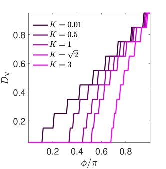
Figure 8: (color online). Vortex density $D_{\text{V}}$ as a function of the effective flux $\phi$ and the interleg coupling $K$ with $N=20$ sites, $g=1$, and the open boundary condition. For each determined $K$, there is a critical value of the flux $\phi_{\text{c}}$. Below $\phi_{\text{c}}$, the system is in the Meissner phase, possessing a constant vortex density $1/N=0.05$, while above $\phi_{\text{c}}$, the system is in the vortex phase, where the vortex density increases with the flux $\phi$.

IV Experimental details

IV.1 Generating the single-particle ground state

To observe the chiral particle current discussed above, we need to generate the single-particle ground state, i.e., the lowest single-particle energy state $|\mu_{1}\rangle$. In principle, the cold atoms can be condensed into one common single-particle state via laser cooling, thus forming the so-called Bose-Einstein condensate. However, since the number of particles here is not conserved as that of atoms, the ladder model realized by superconducting qubit circuits will decay to the ground state (with no particles present) through sufficient cooling of the conventional dilution refrigerator. Hence, in the following, we will demonstrate how to generate the single-particle ground state from the ground state.

We now discuss a general method that generates the single-particle ground state from the ground state $\left|0\right\rangle$, and simultaneously causes no unwanted excitations. In detail, we classically drive the qubits at all the sites, which appears in Eq. (4) as an additional term

$$\hat{H}_{\text{g}}=\frac{\hbar}{2}\sum_{d=\text{L}}^{\text{R}}\sum_{l=1}^{N}\hat{\sigma}_{+}^{\left(d,l\right)}B_{d,l}\exp\left(-i\nu_{d}t\right)+\text{H.c.}.$$ (33)

When we further go to Eq. (11), $\hat{H}_{\text{g}}$ is transformed into

$$\hat{H}_{\text{ld,g}}=\frac{\hbar}{2}\sum_{d=\text{L}}^{\text{R}}\sum_{l=1}^{N}\hat{\sigma}_{+}^{\left(d,l\right)}B_{d,l}^{\prime}\exp\left(-i\epsilon t\right)+\text{H.c.}.$$ (34)

Here, the driving strength $B_{d,l}^{\prime}=B_{d,l}J_{0}\left(\frac{\Omega}{\delta}\right)\approx B_{d,l}$, since $\left|\Omega/\delta\right|^{2}\ll 1$ is satisfied by the parameters in Sec. II, and the detuning $\epsilon\equiv\nu_{d}-\omega_{d}$ for $d=\mathrm{L,R}$ can be achieved via carefully tuning $\nu_{d}$. In Fig. 9, it can be found that the eigenstates are approximately degenerate in pairs when $K<K_{\text{c}}$, although the approximate degeneracy is broken when $K>K_{\text{c}}$. Therefore, when we excite the single-particle ground state $\left|\mu_{1}\right\rangle$ from ground state with $\epsilon=\mu_{1}$, at least the single-particle state $\left|\mu_{2}\right\rangle$ might also be excited and so might the other single-particle states.

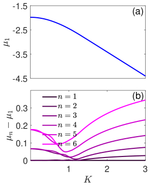
Figure 9: (color online). (a) Ground state frequency versus the interleg coupling $K$. (b) Lowest six eigen frequencies versus $K$ in reference to the ground state frequency. Here, the flux $\phi=\pi/2$, the site number $N=20$, the intraleg coupling $g=1$, and the open boundary condition is assumed. We find the critical value of the interleg coupling $K_{\text{c}}$, below which, the eigen frequencies are nearly degenerate in pairs. However, above $K_{\text{c}}$, the degeneracy is broken.

To overcome this problem, we now make a unitray transformation of the single-particle creation operator, i.e., $\hat{\sigma}_{+}^{\left(d,l\right)}=\sum_{n=1}^{2N}\chi_{d,l}^{\left(n\right)\ast}\hat{\Sigma}_{n}^{+}$, and thus the interaction Hamiltonian in Eq. (34) becomes

$$\hat{H}_{\text{ld,g}}=\frac{\hbar}{2}\sum_{n=1}^{2N}C_{n}\hat{\Sigma}_{n}^{+}\exp\left(-i\epsilon t\right)+\text{H.c.}.$$ (35)

Here, the Pauli operator $\hat{\Sigma}_{n}^{+}$ represents the collective exciations of the qubits, and the driving strength $C_{n}=\sum_{d=\text{L}}^{\text{R}}\sum_{l=1}^{N}\chi_{d,l}^{\left(n\right)\ast}B_{d,l}^{\prime}~{}$can be controlled by the amplitude $B_{d,l}^{\prime}$ (or equivalently, $B_{d,l}$). To remove the excitations on the single-particle excitation states (i.e., the states $\left|\mu_{n}\right\rangle$ with $n\geq 2$), we should make $C_{n}=0$ for $n\geq 2$, which yields the required driving strength

$$B_{d,l}^{\prime}=\sum_{n=1}^{2N}\chi_{d,l}^{\left(n\right)}C_{n}=\chi_{d,l}^{\left(1\right)}C_{1}$$ (36)

using the orthonormality condition of $\chi_{d,l}^{\left(n\right)}$. Obviously, the driving fields $B_{d,l}^{\prime}$ must possess the same profile as the single-particle ground state $\chi_{d,l}^{\left(1\right)}$ except for a scaling factor, i.e., the Rabi frequency $C_{1}$. Then, Eq. (35) can be simplified into

$$\hat{H}_{\text{ld,g}}^{\prime}=\frac{\hbar}{2}C_{1}\exp\left(-i\epsilon t\right)\hat{\Sigma}_{1}^{+}+\mathrm{H.c.},$$ (37)

where we assume $C_{1}$ is tuned positive. From Eqs. (9) and (10), we know that $\hat{\sigma}_{+}^{\left(d,l\right)}\left|0\right\rangle=\hat{b}_{d,l}^{{\dagger}}\left|0\right\rangle$, thus yielding

$$\hat{\Sigma}_{1}^{+}\left|0\right\rangle =\sum_{d=\text{L}}^{\text{R}}\sum_{l=1}^{N}\chi_{d,l}^{\left(1\right)}\hat{\sigma}_{+}^{\left(d,l\right)}\left|0\right\rangle$$

$$=\sum_{d=\text{L}}^{\text{R}}\sum_{l=1}^{N}\chi_{d,l}^{\left(1\right)}\hat{b}_{d,l}^{{\dagger}}\left|0\right\rangle=\left|\mu_{1}\right\rangle.$$ (38)

Since the single-particle ground state is generated from the ground state, we then have

$$\hat{H}_{\text{ld,g}}^{\prime}=\frac{\hbar}{2}C_{1}\exp\left(-i\epsilon t\right)\left|\mu_{1}\right\rangle\!\left\langle 0\right|+\mathrm{H.c.}.$$ (39)

Thus, the unwanted excitations characterized by $C_{n}$ for $n\geq 2$ are all removed via properly adjusting $B_{d,l}^{\prime}$. If the detuning is further taken as $\epsilon=\mu_{1}$ as expected, the system will evolve to the state $\cos\left(C_{1}t/2\right)\!\left|0\right\rangle-i\sin\left(C_{1}t/2\right)\!\left|\mu_{1}\right\rangle$ in a time duration $t$. Assuming a $\pi$ pulse, i.e., $C_{1}t=\pi$, the single-particle ground state $\left|\mu_{1}\right\rangle$ can be achieved in just one step. If we specify the intraleg coupling strength $g/2\pi=3.5\operatorname{MHz}$, the interleg coupling strength $K/2\pi=1.75\operatorname{MHz}$, the ladder length $N=20$, the flux $\phi=\pi/2$, and the detuning $\epsilon/2\pi=\mu_{1}/2\pi=-210.4\operatorname{MHz}$, the driving strength $B_{d,l}^{\prime}$ required to reach the desired Rabi frequencies $C_{1}/2\pi=1\operatorname{MHz}$ and $C_{n}/2\pi=0$ ($n\geq 2$) can be shown in Fig. 10, which implies a generation time of $0.5\operatorname{\mu s}$. Besides, we can verify that $\left|B_{d,l}^{\prime}\right|$ [see Fig. 10(a)] shares the same profile as $\left|\chi_{d,l}^{\left(1\right)}\right|$ [see Figs. 4(a) and  4(b)] except for a scaling factor.

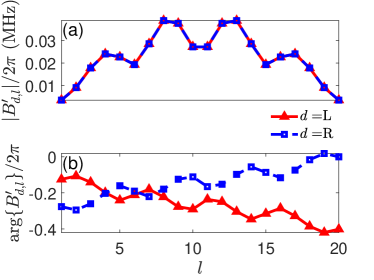
Figure 10: (color online). Driving strength $\left|B_{d,l}^{\prime}\right|/2\pi$ and phase $\arg\{B_{d,l}^{\prime}\}/2\pi$ at the site $(d,l)$ which is needed to reach the Rabi frequency $C_{1}/2\pi=1\operatorname{MHz}$ for generating the single-particle ground state. The solid red (dashed blue) curves marked with triangles (squares) mean $d=\mathrm{L}$ ($d=\mathrm{R}$). Here, the intraleg coupling strength $g/2\pi=3.5\operatorname{MHz}$, the interleg coupling strength $K/2\pi=1.75\operatorname{MHz}$ (such that $K/g=0.5$), the ladder length $N=20$, and the flux $\phi=\pi/2$ are assumed.

Having obtained the target Hamiltonian in Eq. (39), we now investigate the effect of the environment on the state generation process, which is described by the Lindblad master equation

$$\frac{\text{d}\hat{\rho}}{\text{d}t}=\frac{1}{i\hbar}[\hat{H}_{\text{ld}}^{\left(N\right)}+\hat{H}_{\text{ld,g}}^{\prime},\hat{\rho}]+\mathcal{L}_{\mu 1}\left[\hat{\rho}\right].$$ (40)

Here, $\hat{\rho}$ is the density operator of the ladder, $\mathcal{L}_{\mu 1}\left[\hat{\rho}\right]$ represents the Lindblad dissipation terms as

$$\mathcal{L}_{\mu 1}\left[\hat{\rho}\right] =-\gamma_{1}\left|\mu_{1}\right\rangle\!\left\langle\mu_{1}\right|\left\langle\mu_{1}\right|\!\hat{\rho}\!\left|\mu_{1}\right\rangle\!+\!\gamma_{1}\left|0\right\rangle\!\left\langle 0\right|\left\langle 0\right|\!\hat{\rho}\!\left|0\right\rangle\!$$

$$-\!\frac{\Gamma_{1}}{2}\left|\mu_{1}\right\rangle\!\left\langle 0\right|\left\langle\mu_{1}\right|\!\hat{\rho}\!\left|0\right\rangle\!-\!\frac{\Gamma_{1}}{2}\left|\mu_{1}\right\rangle\!\left\langle 0\right|\left\langle\mu_{1}\right|\!\hat{\rho}\!\left|0\right\rangle,$$ (41)

and $\gamma_{1}$ ($\Gamma_{1}$) is the relaxation (dephasing) rate of the single-particle ground state $\left|\mu_{1}\right\rangle$. Using Eq. (40), we can find the exact solution of $\left\langle\mu_{1}\right|\!\hat{\rho}\left(t\right)\!\left|\mu_{1}\right\rangle$ (see Appendix. C), i.e., the fidelity of the single-particle ground state at the time $t$. However, in the strong coupling limit ($C_{1}\gg\gamma_{1}$, $\Gamma_{1}$), the generation fidelity can be approximated as

$$\left\langle\mu_{1}\right|\!\hat{\rho}\!\left|\mu_{1}\right\rangle=\frac{1}{2}\left[1-e^{-\frac{1}{2}\left(\gamma_{1}+\frac{\Gamma_{1}}{2}\right)t}\cos\left(C_{1}t\right)\right].$$ (42)

Suppose the relaxation (dephasing) rate of the qubit at the site $\left(d,l\right)$ is $\gamma_{d,l}$ ($\Gamma_{d,l}$), then $\gamma_{1}$ and $\Gamma_{1}$ can be estimated by

$$\gamma_{1}=\sum_{d,l}|\chi_{d,l}^{\left(1\right)}|^{2}\gamma_{d,l}\text{ and }\Gamma_{1}=\sum_{d,l}|\chi_{d,l}^{\left(1\right)}|^{2}\Gamma_{d,l}.$$ (43)

We consider homogeneous qubit decay rates, e.g., $\gamma_{d,l}/2\pi\equiv 0.05\operatorname{MHz}$ and $\Gamma_{d,l}/2\pi\equiv 0.1\operatorname{MHz}$, while other parameters remain unchanged. Then, after a $\pi~{}$pulse, the fidelity is about $\left\langle\mu_{1}\right|\!\hat{\rho}(\frac{\pi}{C_{1}})\!\left|\mu_{1}\right\rangle=$ $0.9273$. In Fig. 11, we have shown the exact solution and the approximate one for the weak ($\Gamma_{1}=10C_{1}$), critical ($\Gamma_{1}=C_{1}$), and strong ($\Gamma_{1}=0.1C$) coupling, where good agreement is found in the last case.

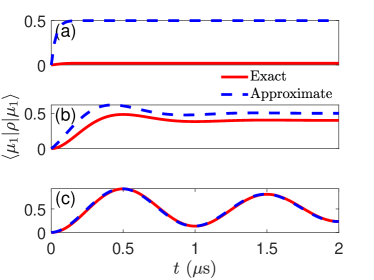
Figure 11: (color online). Single-particle ground state fidelity $\left\langle\mu_{1}\right|\!\hat{\rho}\!\left|\mu_{1}\right\rangle$ evolving versus the time $t$ under the effects of environment for the dephasing rate $\Gamma_{1}$ taking (a) $10C_{1}$, (b) $C_{1}$, and (c) $0.1C_{1}$, respectively. Here, $C_{1}/2\pi=1\operatorname{MHz}$ is the Rabi frequency. The relaxation rate takes $\gamma_{1}=0.5\Gamma_{1}$ in all plots. The solid red (dashed blue) curve denotes the exact solution (the approximate one in the strong coupling limit $C_{1}\gg\gamma_{1},\Gamma_{1}$).

IV.2 Measurement scheme

To observe the vortex-Meissner phase transition, one indispensable issue is to measure the particle currents between a pair of adjacent sites. In superconducting quantum circuits, the qubit state can be dispersively read out by a microwave resonator, which enables us to extract the particle current from the Rabi oscillation between the pair of adjacent sites. To achieve this, we can tune the energy levels of the flux qubits that connect to the pair of sites we concentrate on such that both sites are decoupled from the others. For example, to investigate the Rabi oscillation between $\left(\text{L},l\right)$ and $\left(\text{L},l+1\right)$, we can tune the flux qubits at the sites $\left(\text{L},l-1\right)$, $\left(\text{L},l+2\right)$, $\left(\text{R},l\right)$, and $\left(\text{R},l+1\right)$ such that they are decoupled from the ones at $\left(\text{L},l\right)$ and $\left(\text{L},l+1\right)$. Then, the bare Hamiltonian that governs the evolution of the adjacent sites $\left(\text{L},l\right)$ and $\left(\text{L},l+1\right)$ can be given by $\hat{H}_{\text{L},l}=-\hbar g\hat{\sigma}_{+}^{\left(\text{L},l+1\right)}\hat{\sigma}_{-}^{\left(\text{L},l\right)}+\mathrm{H.c..}$ Differently from the cold atoms in optical lattices, the particles stored in the flux qubits suffer the relaxation rates $\gamma_{d,l}$ and dephasing rates $\Gamma_{d,l}$ for the site $\left(d,l\right)$. Thus, the interaction between the qubits at $\left(\text{L},l\right)$ and $\left(\text{L},l+1\right)$ should also be described by the Lindblad master equation, i.e.,

$$\frac{\text{d}\hat{\rho}_{\text{L},l}}{\text{d}t}=\frac{[\hat{H}_{\text{L},l},\hat{\rho}_{\text{L},l}]}{i\hbar}+\mathcal{L}_{\text{L,}l}\left[\hat{\rho}_{\text{L},l}\right]+\mathcal{L}_{\text{L,}l+1}\left[\hat{\rho}_{\text{L},l}\right].$$ (44)

Here, $\hat{\rho}_{\text{L},l}=\sum_{l_{1}=l}^{l+1}\sum_{l_{2}=l}^{l+1}\left|\text{L,}l_{1}\right\rangle\!\left\langle\text{L,}l_{1}\right|\hat{\rho}\left|\text{L,}l_{2}\right\rangle\!\left\langle\text{L,}l_{2}\right|$ is the subspace truncation of the global density operator $\hat{\rho}$, and the Lindblad terms

$$\mathcal{L}_{\mathrm{L},l}\!\left[\hat{\rho}_{\text{L},l}\right] =-\gamma_{\mathrm{L},l}\left|\mathrm{L},l\right\rangle\!\left\langle\mathrm{L},l\right|\!\left\langle\mathrm{L},l\right|\!\hat{\rho}_{\text{L},l}\!\left|\mathrm{L},l\right\rangle$$

$$+\gamma_{\mathrm{L},l}\left|0\right\rangle\!\left\langle 0\right|\!\left\langle 0\right|\!\hat{\rho}_{\text{L},l}\!\left|0\right\rangle-\frac{\Gamma_{\mathrm{L},l}}{2}\left|0\right\rangle\!\left\langle\mathrm{L},l\right|\!\left\langle 0\right|\!\hat{\rho}_{\text{L},l}\!\left|\mathrm{L},l\right\rangle$$

$$-\frac{\Gamma_{\mathrm{L},l}}{2}\left|\mathrm{L},l\right\rangle\!\left\langle 0\right|\!\left\langle\mathrm{L},l\right|\hat{\rho}_{\text{L},l}\!\left|0\right\rangle$$ (45)

represent the dissipation into the environment. In the limit of strong coupling (i.e., $g\gg\gamma_{\mathrm{L},l},\Gamma_{\mathrm{L},l}$), the population difference between $\left(\text{L},l+1\right)$ and $\left(\text{L},l\right)$, which defined by $P_{\text{L,}l}\left(t\right)=\left\langle\text{L},l+1\right|\!\hat{\rho}_{\text{L},l}\!\left|\text{L},l+1\right\rangle-\left\langle\text{L},l\right|\!\hat{\rho}_{\text{L},l}\!\left|\text{L},l\right\rangle$, can be obtained using the Lindblad master equation as

$$P_{\text{L,}l}\left(t\right)\!=\!e^{-\tilde{\gamma}_{\text{L,}l}t}\!\left[\cos\left(\tilde{g}t\right)\!P_{\text{L,}l}\!\left(0\right)+\sin\left(\tilde{g}t\right)\!\frac{j_{l,l+1}^{\left(\text{L}\right)}}{g}\right],$$ (46)

where $\tilde{\gamma}_{\text{L},l}=\left(\gamma_{\text{L,}l}+\gamma_{\text{L,}l+1}+\Gamma_{\text{L,}l}+\Gamma_{\text{L,}l+1}\right)/4$ and $\tilde{g}=2g$. Now, we can confidently assert that the particle current $j_{l,l+1}^{\left(\text{L}\right)}$ can be extracted from the population difference after fitting the measured data using Eq. (46). The discussions made above can also apply to extracting the particle current on the R leg, for which, the population difference between $\left(\text{R},l\right)$ and $\left(\text{R},l+1\right)$ is namely Eq. (46) with the subscript L replaced with R. Similarly, the population difference between $\left(\text{R},l\right)$ and $\left(\text{L},l\right)$ is

$$P_{\text{LR,}l}\!\left(t\right)=e^{-\tilde{\gamma}_{\text{LR,}l}t}\!\!\left[\cos(\tilde{K}t)P_{\text{LR,}l}\!\left(0\right)+\sin(\tilde{K}t)\frac{j_{\text{LR},l}}{K}\right]\!\text{,}$$ (47)

where $\tilde{\gamma}_{\text{LR},l}=\left(\gamma_{\text{L,}l}+\gamma_{\text{R,}l}+\Gamma_{\text{L,}l}+\Gamma_{\text{R,}l}\right)/4$, $\tilde{K}=2K$, and strong interleg coupling (i.e., $K\gg\gamma_{\mathrm{L},l},\Gamma_{\mathrm{L},l}$) has been assumed.

In Fig. 12, we have intuitively presented the population difference $P_{\text{L,}l}\left(t\right)$ and $P_{\text{LR,}l}\left(t\right)$ evolving as the time for $l$ taking $N/2$, with the chain length $N=20$, the intraleg coupling strength $g/2\pi=3.5\operatorname{MHz}$, the interleg coupling strength $K/2\pi=1.75\operatorname{MHz}$ (such that $K/g=0.5$), the effective magnetic flux $\phi=\pi/2$, and the decay rates $\gamma_{d,l^{\prime}}/2\pi\equiv 0.05\operatorname{MHz}$ and $\Gamma_{d,l^{\prime}}/2\pi\equiv 0.1\operatorname{MHz}$. The corresponding particle current is $j_{l,l+1}^{\left(\text{L}\right)}=0.43\operatorname{MHz}$ and $j_{\text{LR},l}=-0.5785\operatorname{MHz}$. We find that, in the strong coupling limit, the approximate analytical solutions (solid blue) agree very well with the exact numerical simulation results (dashed green), especially in the first few periods. However, when time goes longer, some deviation is exhibited from the approximate and numerical results. Thus, to improve accuracy of measurement, we advice to fit the data from the first few oscillation periods.

Having measured the particle currents between adjacent sites, we can then calculate the chiral current given in Eq. (32), which enables us to obtain the vortex-Meissner phase transition diagram for different interleg coupling strength $K$ and effective magnetic flux $\phi$ (see Fig. 6). The current patterns (see Fig. 7) can also be obtained from the particle currents, which enables us to calculate the vortex density for different $K$ and $\phi$ (see Fig. 8). In a word, the vortex-Meissner phase transition can be determined from the measured data of particle currents between adjacent sites.

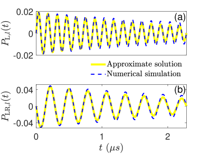
Figure 12: (color online). Population difference (a) $P_{\text{L,}l}\left(t\right)$ between the site ($\mathrm{L},l+1$) and ($\mathrm{L},l$), and (b) $P_{\text{LR},l}\left(t\right)$ between the site ($\mathrm{R},l$) and ($\mathrm{L},l$) evolving against the time $t$. The solid yellow (dashed blue) curves represents the exact numerical simulation results (approximate solutions) in the strong coupling limit. Here, we specify the chain length $N=20$, the lattice index $l=N/2=10$, the intraleg coupling strength $g/2\pi=3.5\operatorname{MHz}$, the interleg coupling strength $K/2\pi=1.75\operatorname{MHz}$, and the decay rates at the site $(d,l^{\prime})$ $\gamma_{d,l^{\prime}}/2\pi\equiv 0.05\operatorname{MHz}$ and $\Gamma_{d,l^{\prime}}/2\pi\equiv 0.1\operatorname{MHz}$. The corresponding particle current is (a) $j_{l,l+1}^{\left(\text{L}\right)}=0.43\operatorname{MHz}$ and (b) $j_{\text{LR},l}=-0.5785\operatorname{MHz}$.

V Conclusion

We have introduced a circuit scheme on how to construct the two-leg fermionic ladder with X-shape gradiometer superconducting flux qubits. In such a scheme, we have shown that with two-tone driving fields, an artificial effective magnetic flux can be generated for each plaquette, which can be felt by the “fermionic” particle and thus affects its motion. Compared with the previous method for generating effective magnetic flux without the aid of couplers Alaeian2019PRA , our method does not require the qubit circuit poessess a weak anharmonicity but on the contrary has a simple analytical expression in the strong anharmonicity regime. The maintenance of anharmonicity (or nonlinearity) is crucial, since it is indispensable for demonstrating quantum behaviors  Wendin2007LTP .

Via modifying the interleg coupling strength or the effective magnetic flux, both of which are tunable via adjusting the phases of the classical driving fields, the vortex-Meissner phase transition can in principle be observed in the single-particle ground state, which originates from the competition between the two parameters. In the vortex phase, the number of vortex kernels are more than one, while in the Meissner phase, there is only one large vortex, with the currents mainly flowing around the boundaries of the ladder. The phase transition boundary is analytically given. Besides, the wave functions, current patterns, and quasimomentum distributions in both phases are exhaustively discussed. The vortex densities for different parameters have also been presented.

Since the vortex and Meissner phases are discussed in the single-particle ground state, which is not the (global) ground state, we have proposed a method on how to generate the single-particle ground state from the ground state with just a one-step $\pi$ pulse realized by simultaneously driving all the qubits and meanwhile cause no undesired excitations. The requied driving fields should share the same profile as the wave function of the single-particle ground state except for a scaling factor, the Rabi frequency of generation.

We have shown that the particle currents between the two adjacent sites can be extracted from the Rabi oscillations between them, assuming the other sites connected to them are tuned to decouple. The detailed analytical expression has been given for fitting the experimentally measured data. The particle-current measurement between adjacent sites enables the calculation of chiral particle currents, which is critical for experimentally determining the vortex-Meissner phase transition.

For strictness, the effects of the environment are also considered for generating the single-particle ground state and measuring the particle currents between the adjacent sites. To guarantee the generation fidelity and measurement accuracy, we find that the sample needs to reach the strong coupling regime, i.e., the coupling strength should be much larger than the decay rates. This condition, we think, should not be very difficult to met, since the ultrastrong coupling Niemczyk2010NP ; Forn2016NP ; Yoshihara2017NP and decoherence time about tens of microseconds Yan2016NC ; Abdurakhimov2019APL have both been reported in flux qubit systems.

VI Acknowledgments

We are grateful to Wei Han for helpful discussions. Y. J. Z. is supported by National Natural Science Foundation of China (NSFC) under grants No.s 11904013 and 11847165. Y.X.L. is supported by the Key-Area Research and Development Program of GuangDong Province under Grant No.2018B030326001, the National Basic Research Program(973) of China under Grant No. 2017YFA0304304. W. M. L. was supported by the National Key R&D Program of China under grants No. 2016YFA0301500, NSFC under grants Nos. 61835013, Strategic Priority Research Program of the Chinese Academy of Sciences under grants Nos. XDB01020300, XDB21030300.

Appendix A Periodical modulation of the qubit frequency

Now, we investigate the periodical modulation of a qubit frequency with a general qubit (e.g., flux qubit, transmon qubit, etc) with multiple energy levels. The qubit Hamiltonian with two-tone driving fields can be represented as

$$\hat{H}_{\text{q}}=\hat{H}_{0}+\frac{\hbar}{2}\sum_{n}^{N-1}\sum_{j=1}^{2}\left(\hat{\sigma}_{n+1,n}\Omega_{jn}e^{-i\tilde{\omega}_{j}t}+\mathrm{H.c.}\right),$$ (48)

where $\hat{H}_{0}=\sum_{n}\hbar\omega_{qn}\hat{\sigma}_{nn}$ and $\hat{\sigma}_{nn}=\left|n\right\rangle\left\langle n\right|$ ($\hat{\sigma}_{n+1,n}=\left|n+1\right\rangle\left\langle n\right|)$ is the projection (ladder) operator. In the interaction picture defined by $\hat{U}_{0}\left(t\right)=e^{-i\hat{H}_{0}t}$, the Hamiltonian $\hat{H}_{\text{q}}$ is transformed into

$$\hat{H}_{\text{I}}\left(t\right)=\frac{\hbar}{2}\sum_{n}^{N-1}\sum_{j=1}^{2}\left(\hat{\sigma}_{n+1,n}\Omega_{jn}e^{-i\delta_{jn}t}+\mathrm{H.c.}\right)\text{,}$$ (49)

where $\delta_{jn}=\tilde{\omega}_{j}-\left(\omega_{q,n+1}-\omega_{q,n}\right)$ is the detuning between the driving field and the applied energy level.

To derive the effective Hamiltonian, we employ the second-order perturbation theory in the large-detuning regime $\left|\Omega_{jn}/\delta_{j^{\prime}n}\right|^{2}\ll 1$, thus resulting in the evolution operator in the interaction as

$$\hat{U}_{\text{I}}\left(t\right)\cong 1+\frac{1}{i\hbar}\int_{0}^{t}\text{d}t^{\prime}\hat{H}_{\text{I}}\left(t^{\prime}\right)$$

$$+\frac{1}{\left(i\hbar\right)^{2}}\int_{0}^{t}\text{d}t^{\prime}\hat{H}_{\text{I}}\left(t^{\prime}\right)\int_{0}^{t^{\prime}}\hat{H}_{\text{I}}\left(t^{\prime\prime}\right)\text{d}t^{\prime\prime}.$$ (50)

In the time scale $t\gtrsim\frac{1}{\left|\Omega_{jn}\right|}$, which satisfies $t\gg\frac{1}{\left|\delta_{jn}\right|}$, the fast-oscillating term (i.e., the first-order perturbative term) in Eq. (50) can be neglected, thus resulting in

$$\hat{U}_{\text{I}}\cong 1\!+\frac{1}{i^{2}}\sum_{n=0}^{N-1}\int_{0}^{t}\text{d}t^{\prime}\sum_{j=1}^{2}\frac{\left|\Omega_{jn}\right|^{2}}{4}\left(\frac{\hat{\sigma}_{n+1,n+1}}{i\delta_{jn}}-\frac{\hat{\sigma}_{n,n}}{i\delta_{jn}}\right)$$

$$+\frac{1}{4i^{2}}\sum_{n=0}^{N-1}\int_{0}^{t}\text{d}t^{\prime}\left(\frac{O_{n}}{i\delta_{1n}}\hat{\sigma}_{n+1,n+1}-\frac{O_{n}^{\ast}}{i\delta_{1n}}\hat{\sigma}_{n,n}\right)$$

$$+\!\frac{1}{4i^{2}}\!\sum_{n=0}^{N-1}\!\int_{0}^{t}\text{d}t^{\prime}\!\left(\frac{O_{n}^{\ast}}{i\delta_{2n}}\hat{\sigma}_{n+1,n+1}-\hat{\sigma}_{n,n}\frac{O_{n}}{i\delta_{2n}}\right)\!,$$ (51)

where the symbol $O_{n}\equiv O_{n}\left(t\right)=$ $\Omega_{1n}^{\ast}\Omega_{2n}e^{-i\tilde{\delta}t}$ and the detuning $\tilde{\delta}=$ $\delta_{2n}-\delta_{1n}=\tilde{\omega}_{2}-\tilde{\omega}_{1}$. Assuming $|\tilde{\delta}|\ll\left|\delta_{jn}\right|$, which implies $\delta_{1n}\approx\delta_{2n}$, we can obtain the effective Hamiltonian using the relation $H_{\text{I,eff}}=i\hbar\partial_{t}U_{\text{I}}\left(t\right)$ as

$$\hat{H}_{\text{I,eff}} =\sum_{j=1}^{2}\frac{\hbar\left|\Omega_{j0}\right|^{2}}{4\delta_{j0}}\hat{\sigma}_{00}$$

$$+\sum_{n=0}^{N-1}\sum_{j}\left(\frac{\hbar\left|\Omega_{j,n+1}\right|^{2}}{4\delta_{j,n+1}}-\frac{\hbar\left|\Omega_{jn}\right|^{2}}{4\delta_{jn}}\right)\hat{\sigma}_{n+1,n+1}$$

$$-\sum_{n=0}^{N-1}\frac{\hbar}{2}\frac{\left|\Omega_{1n}\Omega_{2n}\right|}{\delta_{1n}}\hat{\sigma}_{n+1,n+1}\cos\left(\tilde{\delta}t+\phi_{n}\right)$$

$$+\sum_{n=0}^{N-1}\frac{\hbar}{2}\frac{\left|\Omega_{1n}\Omega_{2n}\right|}{\delta_{1n}}\hat{\sigma}_{nn}\cos\left(\tilde{\delta}t+\phi_{n}\right),$$ (52)

where we have defined $\phi_{1n}-\phi_{2n}\equiv\phi_{n}$. Omitting an irrelevant constant, the effective Hamiltonian can be further represented as

$$\hat{H}_{\text{I,eff}}\cong\sum_{n=1}^{N}\hbar\left[\nu_{n}+\eta_{n}\cos\left(\tilde{\delta}t+\phi_{n-1}\right)\right]\hat{\sigma}_{n,n},$$ (53)

where $\nu_{n}$ is the Stark shift and $\eta_{n}$ is the periodical modulation strength:

$$\nu_{n} =\sum_{j=1}^{2}\frac{\left|\Omega_{jn}\right|^{2}}{4\delta_{jn}}-\frac{\left|\Omega_{j,n-1}\right|^{2}}{4\delta_{j,n-1}}-\frac{\left|\Omega_{j0}\right|^{2}}{4\delta_{j0}},$$ (54)

$$\eta_{n} =\!\frac{1}{2}\!\left(\frac{\left|\Omega_{1n}\Omega_{2n}\right|}{\delta_{1n}}\!-\frac{\left|\Omega_{1,n-1}\Omega_{2,n-1}\right|}{\delta_{1,n-1}}\!-\frac{\left|\Omega_{10}\Omega_{20}\right|}{\delta_{10}}\right)\!.$$ (55)

Returning to the original frame, the effective Hamiltonian is transformed into the form

$$\hat{H}_{\text{eff}}\cong\sum_{n=1}^{N}\hbar\left[\tilde{\omega}_{qn}+\eta_{n}\cos\left(\tilde{\delta}t+\phi_{n-1}\right)\right]\hat{\sigma}_{n,n},$$ (56)

where $\tilde{\omega}_{qn}=\omega_{qn}+\nu_{n}$. In the large-detuning regime, the Stark shift $\nu_{n}$ is a small quantity compared to $\omega_{qn}$.

If the qubit circuit possesses adequate anharmonicity, and all the control pulses involved are carefully designed to avoid the excitation to higher energy levels, then the Hamiltonian can be confined to the single-particle case, thus arriving at

$$\hat{H}_{\text{eff}}=\hbar\omega_{q1}\hat{\sigma}_{11}+\hbar\eta_{1}\cos\left(\tilde{\delta}t+\phi_{0}\right)\hat{\sigma}_{11}.$$ (57)

If we further focus on the flux qubit circuit which is typically treated as an ideal two-level system where $\delta_{11}=\infty$, we have a simple result $\eta_{1}\approx-\frac{\left|\Omega_{10}\Omega_{20}\right|}{\delta_{10}}$ and then $\hat{H}_{\text{eff}}$ becomes the form of Eq. (3).

Now, we discuss the limit that the anharmonicity of the qubit is so weak that Eq. (48) becomes the form of a driven resonator. In this case, the parameters can be represented as $\omega_{n}=n\bar{\omega}$, $\Omega_{jn}=\sqrt{n+1}\bar{\Omega}_{j}$, and $\delta_{jn}=Const,$ where $\bar{\omega}$ is the fundamental frequency of the resonator and $\bar{\Omega}_{j}$ is the driving strength on the resonator. Using such parameters, one can obtain that the Stark shift $\nu_{n}=0$ and $\eta_{n}=0$, and thus the periodical modulation of the qubit frequency vanishes. Therefore, to achieve the periodical modulation using two-tone driving fields, the superconducting qubit circuit should maintain a nonzero anharmonicity. In principle, the periodical modulation effect shall exist only if the anharmonicity of the interested qubit circuit is nonzero. This character requires a wider anharmonicity range of the qubit circuit than in Ref. Alaeian2019PRA , where the anharmonicity of the transmon qubit circuit needs to be negligibly small. Since the nonlinearity is a key factor for demonstrating quantum phenomena Wendin2007LTP , we think periodically modulating the qubit circuit with better anharmonicity is significant for exploring nonequilibrium quantum physics.

Appendix B Treatment into the interaction picture

The full Hamiltonian with periodically modulated qubit frequency is given by

$$\hat{H}_{\text{f}}= \sum_{l}\sum_{d=\text{L,R}}\left[\frac{\hbar}{2}\omega_{d}\sigma_{z}^{\left(d,l\right)}-\frac{\hbar}{2}\Omega\cos\left(\delta t+\phi_{d,l}\right)\sigma_{z}^{\left(\text{L},l\right)}\right]$$

$$-\sum_{l}\hbar g\sigma_{-}^{\left(d,l\right)}\sigma_{+}^{\left(d,l+1\right)}+\text{H.c.},$$

$$-\sum_{l}\hbar K\sigma_{-}^{\left(\text{L},l\right)}\sigma_{+}^{\left(\text{R},l\right)}+\text{H.c.}$$ (58)

where the subscript L and R represent the left and right legs of the ladder, $l$ the lattice site, $\omega_{d}$ ($d=\mathrm{L,R}$) the qubit frequency on the leg $d$, $g$ the intraleg tunneling rate, and $K$ the interleg tunneling rate. To eliminate the time-dependent terms in Eq. (4), we now apply to Eq. (4) a unitary transformation $U_{d}\left(t\right)={\textstyle\prod\limits_{l}}{\textstyle\prod\limits_{d=\mathrm{L,R}}}\exp\left[iF_{l,d}\left(t\right)\right]$ with

$$F_{l,d}\left(t\right)=\frac{\sigma_{z}^{\left(d,l\right)}}{2}\left[\frac{\Omega}{\delta}\sin\left(\delta t+\phi_{d,l}\right)+\omega_{d}t\right],$$ (59)

in which manner, we now enter the interaction picture, and obtain the effective Hamiltonian as

$$\hat{H}_{\text{f}}= -\sum_{l}\sum_{d=\mathrm{L,R}}\left[\hbar g\sigma_{-}^{\left(\text{L},l\right)}\sigma_{+}^{\left(\text{L},l+1\right)}e^{i\alpha_{\text{L},l}\left(t\right)}+\text{H.c.}\right]$$

$$-\sum_{l}\sum_{d=\mathrm{L,R}}\left[\hbar g\sigma_{-}^{\left(\text{L},l\right)}\sigma_{+}^{\left(\text{L},l+1\right)}e^{i\alpha_{\text{R},l}\left(t\right)}+\text{H.c.}\right]$$

$$-\sum_{l}\left[\hbar K\sigma_{-}^{\left(\text{L},l\right)}\sigma_{+}^{\left(\text{R},l\right)}e^{i\beta_{l}\left(t\right)}+\text{H.c.}\right]\text{.}$$ (60)

Here, the phase parameters $\alpha_{d,l}\left(t\right)$ and $\beta_{l}\left(t\right)$ are

$$\alpha_{d,l}\left(t\right) =\left[\frac{2\Omega}{\delta}\sin\phi_{d,l}^{\left(-\right)}\right]\cos\left(\delta t+\phi_{d,l}^{\left(+\right)}\right),d=\text{L,R}$$ (61)

$$\beta_{l}\left(t\right) =\left[\frac{2\Omega}{\delta}\sin\phi_{l}^{\left(-\right)}\right]\cos\left(\delta t+\phi_{l}^{\left(+\right)}\right)+\Delta,$$ (62)

where $\phi_{d,l}^{\left(\pm\right)}=\left(\phi_{d\text{,}l}\pm\phi_{d\text{,}l+1}\right)/2$, $\phi_{l}^{\left(\pm\right)}=\left(\phi_{\text{L,}l}\pm\phi_{\text{R,}l+1}\right)/2$, and $\Delta=\omega_{\text{R}}-\omega_{\text{L}}$ is the qubit frequency difference between different legs. Furthermore, we define $\phi_{d\text{,}l}=\phi_{d}-\phi l$, $\phi_{\text{L}}=-\phi_{\text{R}}=\phi_{0}$, and use the relation $\exp\left(ix\sin\theta\right)=\sum_{n}J_{n}\left(x\right)e^{in\theta}$, where $J_{n}\left(x\right)$ is the $n$th Bessel function of the first kind, which yields the Hamiltonian as Liu2014NJP ; Zhao2015PRA

$$\hat{H}_{\text{f}}^{\prime}= -\sum_{ln}\hbar g_{0}\sigma_{-}^{\left(\text{L},l\right)}\sigma_{+}^{\left(\text{L},l+1\right)}J_{xnl}^{\left(+\right)}\left(t\right)+\text{H.c.}$$

$$-\sum_{ln}\hbar g_{0}\sigma_{-}^{\left(\text{R},l\right)}\sigma_{+}^{\left(\text{R},l+1\right)}J_{xnl}^{\left(-\right)}\left(t\right)+\text{H.c.}$$

$$-\sum_{ln}\hbar K_{0}\sigma_{-}^{\left(\text{L},l\right)}\sigma_{+}^{\left(\text{R},l\right)}J_{ynl}\left(t\right)+\text{H.c..}$$ (63)

Here, the parameters $J_{xnl}^{\left(\pm\right)}\left(t\right)$ and $J_{ynl}\left(t\right)$ can be explicitly given by

$$J_{xnl}^{\left(\pm\right)} =i^{N}J_{n}\left(\eta_{x}\right)\exp\left[in\left(\delta t\pm\phi_{0}-\phi l-\frac{\phi}{2}\right)\right],$$ (64)

$$J_{ynl} =i^{N}J_{n}\left(\eta_{y}\right)\exp\left[in\left(\delta t-\phi l\right)+i\Delta t\right].$$ (65)

where $\eta_{x}=\frac{2\Omega}{\delta}\sin\left(\frac{\phi}{2}\right)$, $\eta_{y}=\frac{2\Omega}{\delta}\sin\left(\phi_{0}\right)$, and $J_{n}\left(\cdot\right)$ is the Bessel function of the first kind. We now assume the detuning $\delta$ is tuned to match $\Delta$, i.e., $\delta=\Delta$, such that, neglecting fast-oscillating terms, we can obtain the effective Hamiltonian

$$\hat{H}_{\text{ld}}= -\sum_{l}\sum_{d=\text{L,R}}\hbar g\sigma_{-}^{\left(d,l\right)}\sigma_{+}^{\left(d,l+1\right)}+\text{H.c.}$$

$$-\sum_{l}\hbar K\sigma_{-}^{\left(\text{L},l\right)}\sigma_{+}^{\left(\text{R},l\right)}\exp\left(i\phi l\right)+\text{H.c.,}$$ (66)

where $g=g_{0}J_{0}\left(\eta_{x}\right)$ and $K=K_{0}J_{1}\left(\eta_{y}\right)$ can be tunable in principle via modifying the two-tone driving strength $\Omega$.

Appendix C Exact solution of the fidelity with the environment

As the main text demonstrates, the effect of the environment on the state generation process can be described by the Lindblad master equation

$$\frac{\text{d}\hat{\rho}}{\text{d}t}=\frac{1}{i\hbar}\left[\hat{H}_{\text{ld}}^{\left(N\right)}+\hat{H}_{\text{ld,g}}^{\prime},\hat{\rho}\right]+\mathcal{L}_{\mu 1}\left[\hat{\rho}\right].$$ (67)

Here, $\hat{\rho}$ is the density operator of the ladder, $\mathcal{L}_{\mu 1}\left[\hat{\rho}\right]$ represents the Lindblad dissipation terms as

$$\mathcal{L}_{\mu 1}\left[\hat{\rho}\right] =-\gamma_{1}\left|\mu_{1}\right\rangle\!\left\langle\mu_{1}\right|\left\langle\mu_{1}\right|\!\hat{\rho}\!\left|\mu_{1}\right\rangle\!+\!\gamma_{1}\left|0\right\rangle\!\left\langle 0\right|\left\langle 0\right|\!\hat{\rho}\!\left|0\right\rangle\!$$

$$-\!\frac{\Gamma_{1}}{2}\left|\mu_{1}\right\rangle\!\left\langle 0\right|\left\langle\mu_{1}\right|\!\hat{\rho}\!\left|0\right\rangle\!-\!\frac{\Gamma_{1}}{2}\left|\mu_{1}\right\rangle\!\left\langle 0\right|\left\langle\mu_{1}\right|\!\hat{\rho}\!\left|0\right\rangle,$$ (68)

and $\gamma_{1}$ ($\Gamma_{1}$) is the relaxation (dephasing) rate of the single-particle ground state $\left|\mu_{1}\right\rangle$. Solving Eq. (67), where the Hilbert space is $\left\{\left|0\right\rangle,\left|\mu_{1}\right\rangle\right\}$, we can obtain the population on $\left|\mu_{1}\right\rangle$ after some time $t$, i.e.,

$$\rho_{11} =\left\langle\mu_{1}\right|\!\hat{\rho}\!\left|\mu_{1}\right\rangle$$

$$=r_{0}-r_{0}\operatorname{Re}\left\{\left(1-\frac{i\gamma_{1}^{\prime}}{2C_{1}^{\prime}}\right)e^{-\frac{1}{2}\gamma_{1}^{\prime}t}\exp\left(itC_{1}^{\prime}\right)\right\}\!.$$ (69)

Here, the intermediate parameters are explicitly given as follows,

$$r_{0} =\frac{\frac{C_{1}^{2}}{2}}{C_{1}^{2}+\frac{\gamma_{1}\Gamma_{1}}{2}},$$ (70)

$$C_{1}^{\prime} =\sqrt{C_{1}^{2}-\frac{1}{4}\left(\gamma_{1}-\frac{\Gamma_{1}}{2}\right)^{2}},$$ (71)

$$\gamma_{1}^{\prime} =\gamma_{1}+\frac{\Gamma_{1}}{2},$$ (72)

and $\rho_{11}$ is also called the fidelity of $\left|\mu_{1}\right\rangle$. In the limit of strong coupling ($C_{1}\gg\gamma_{1}$, $\Gamma_{1}$), $r_{0}=\frac{1}{2}$, $C_{1}^{\prime}=C_{1}$, and $\gamma_{1}^{\prime}/C_{1}^{\prime}=0$, thus yielding

$$\rho_{11}=\frac{1}{2}\left[1-e^{-\frac{1}{2}\gamma_{1}^{\prime}t}\cos\left(C_{1}t\right)\right],$$ (73)

which yields $\rho_{11}=\frac{1}{2}$ in the steady state ($t=\infty$).

References

- (1) J. D. Jackson, Classical Electrodynamics (John Wiley & Sons, Inc, United States of America, 1999).
- (2) M. K. Gaillard, P. D. Grannis, and F. J. Sciulli, The Standard Model of Particle Physics, Rev. Mod. Phys. 71, S96 (1999).
- (3) M. Z. Hasan and C. L. Kane, Colloquium: Topological Insulators, Rev. Mod. Phys. 82, 3045 (2010).
- (4) Y. Makhlin, G. Schön, and A. Shnirman, Quantum-State Engineering with Josephson-Junction Devices, Rev. Mod. Phys. 73, 357 (2001).
- (5) J. Q. You and F. Nori, Superconducting Circuits and Quantum Information, Phys. Today 58, 42 (2005).
- (6) G. Wendin and V. S. Shumeiko, Quantum Bits with Josephson Junctions (Review Article), Low Temp. Phys. 33, 724 (2007).
- (7) J. Clarke and F. K. Wilhelm, Superconducting Quantum Bits, Nature 453, 1031 (2008).
- (8) R. J. Schoelkopf and S. M. Girvin, Wiring up Quantum Systems, Nature 451, 664 (2008).
- (9) I. Buluta, S. Ashhab, and F. Nori, Natural and Artificial Atoms for Quantum Computation, Rep. Prog. Phys. 74, 104401 (2011).
- (10) J. Q. You and F. Nori, Atomic Physics and Quantum Optics Using Superconducting Circuits, Nature 474, 589 (2011).
- (11) Z.-L. Xiang, S. Ashhab, J. You, and F. Nori, Hybrid Quantum Circuits: Superconducting Circuits Interacting with Other Quantum Systems, Rev. Mod. Phys. 85, 623 (2013).
- (12) X. Gu, A. F. Kockum, A. Miranowicz, Y.-X. Liu, and F. Nori, Microwave Photonics with Superconducting Quantum Circuits, Phys. Rep. 718-719, 1 (2017).
- (13) J. Koch, A. A. Houck, K. L. Hur, and S. M. Girvin, Time-Reversal-Symmetry Breaking in Circuit-QED-Based Photon Lattices, Phys. Rev. A 82, 043811 (2010).
- (14) A. Nunnenkamp, J. Koch, and S. M. Girvin, Synthetic Gauge Fields and Homodyne Transmission in Jaynes-Cummings Lattices, New J. Phys. 13, 095008 (2011).
- (15) D. Marcos, P. Rabl, E. Rico, and P. Zoller, Superconducting Circuits for Quantum Simulation of Dynamical Gauge Fields, Phys. Rev. Lett. 111, 110504 (2013).
- (16) Z.-H. Yang, Y.-P. Wang, Z.-Y. Xue, W.-L. Yang, Y. Hu, J.-H. Gao, and Y. Wu, Circuit Quantum Electrodynamics Simulator of Flat Band Physics in a Lieb Lattice, Phys. Rev. A 93, 062319 (2016).
- (17) P. Roushan, C. Neill, A. Megrant, Y. Chen, R. Babbush, R. Barends, B. Campbell, Z. Chen, B. Chiaro, A. Dunsworth, A. Fowler, E. Jeffrey, J. Kelly, E. Lucero, J. Mutus, P. J. J. O’Malley, M. Neeley, C. Quintana, D. Sank, A. Vainsencher, J. Wenner, T. White, E. Kapit, H. Neven, and J. Martinis, Chiral Ground-State Currents of Interacting Photons in a Synthetic Magnetic Field, Nat. Phys. 13, 146 (2017).
- (18) M. Aidelsburger, M. Atala, S. Nascimbène, S. Trotzky, Y. A. Chen, and I. Bloch, Experimental Realization of Strong Effective Magnetic Fields in an Optical Lattice, Phys. Rev. Lett. 107, 255301 (2011).
- (19) M. Aidelsburger, M. Atala, M. Lohse, J. T. Barreiro, B. Paredes, and I. Bloch, Realization of the Hofstadter Hamiltonian with Ultracold Atoms in Optical Lattices, Phys. Rev. Lett. 111, 185301 (2013).
- (20) H. Miyake, G. A. Siviloglou, C. J. Kennedy, W. C. Burton, and W. Ketterle, Realizing the Harper Hamiltonian with Laser-Assisted Tunneling in Optical Lattices, Phys. Rev. Lett. 111, 185302 (2013).
- (21) M. Atala, M. Aidelsburger, M. Lohse, J. T. Barreiro, B. Paredes, and I. Bloch, Observation of Chiral Currents with Ultracold Atoms in Bosonic Ladders, Nat. Phys. 10, 588 (2014).
- (22) H. Alaeian, C. W. S. Chang, M. V. Moghaddam, C. M. Wilson, E. Solano, and E. Rico, Creating Lattice Gauge Potentials in Circuit Qed: The Bosonic Creutz Ladder, Phys. Rev. A 99, 053834 (2019).
- (23) R. Barends, J. Kelly, A. Megrant, A. Veitia, D. Sank, E. Jeffrey, T. C. White, J. Mutus, A. G. Fowler, B. Campbell, Y. Chen, Z. Chen, B. Chiaro, A. Dunsworth, C. Neill, P. O’Malley, P. Roushan, A. Vainsencher, J. Wenner, A. N. Korotkov, A. N. Cleland, and J. M. Martinis, Superconducting Quantum Circuits at the Surface Code Threshold for Fault Tolerance, Nature 508, 500 (2014).
- (24) Y. Zheng, C. Song, M.-C. Chen, B. Xia, W. Liu, Q. Guo, L. Zhang, D. Xu, H. Deng, K. Huang, Y. Wu, Z. Yan, D. Zheng, L. Lu, J.-W. Pan, H. Wang, C.-Y. Lu, and X. Zhu, Solving Systems of Linear Equations with a Superconducting Quantum Processor, Phys. Rev. Lett. 118, 210504 (2017).
- (25) C. Song, K. Xu, W. Liu, C.-p. Yang, S.-B. Zheng, H. Deng, Q. Xie, K. Huang, Q. Guo, L. Zhang, P. Zhang, D. Xu, D. Zheng, X. Zhu, H. Wang, Y. A. Chen, C. Y. Lu, S. Han, and J.-W. Pan, 10-Qubit Entanglement and Parallel Logic Operations with a Superconducting Circuit, Phys. Rev. Lett. 119, 180511 (2017).
- (26) M. Gong, M.-C. Chen, Y. Zheng, S. Wang, C. Zha, H. Deng, Z. Yan, H. Rong, Y. Wu, S. Li, F. Chen, Y. Zhao, F. Liang, J. Lin, Y. Xu, C. Guo, L. Sun, A. D. Castellano, H. Wang, C. Peng, C.-Y. Lu, X. Zhu, and J.-W. Pan, Genuine 12-Qubit Entanglement on a Superconducting Quantum Processor, Phys. Rev. Lett. 122, 110501 (2019).
- (27) P. J. Leek, J. M. Fink, A. Blais, R. Bianchetti, M. Göppl, J. M. Gambetta, D. I. Schuster, L. Frunzio, R. J. Schoelkopf, and A. Wallraff, Observation of Berry’s Phase in a Solid-State Qubit, Science 318, 1889 (2007).
- (28) S. Berger, M. Pechal, S. Pugnetti, A. A. Abdumalikov, L. Steffen, A. Fedorov, A. Wallraff, and S. Filipp, Geometric phases in superconducting qubits beyond the two-level approximation, Phys. Rev. B 85, 220502 (2012).
- (29) S. Berger, M. Pechal, A. A. Abdumalikov, C. Eichler, L. Steffen, A. Fedorov, A. Wallraff, and S. Filipp, Exploring the effect of noise on the Berry phase, Phys. Rev. A 87, 060303 (2013).
- (30) M. D. Schroer, M. H. Kolodrubetz, W. F. Kindel, M. Sandberg, J. Gao, M. R. Vissers, D. P. Pappas, A. Polkovnikov, and K. W. Lehnert, Measuring a topological transition in an artificial spin-1/2 system, Phys. Rev. Lett. 113, 050402 (2014).
- (31) Z. Zhang, T. Wang, L. Xiang, J. Yao, J. Wu, and Y. Yin, Measuring the Berry phase in a superconducting phase qubit by a shortcut to adiabaticity, Phys. Rev. A 95, 042345 (2017).
- (32) P. Roushan, C. Neill, Y. Chen, M. Kolodrubetz, C. Quintana, N. Leung, M. Fang, R. Barends, B. Campbell, Z. Chen, B. Chiaro, A. Dunsworth, E. Jeffrey, J. Kelly, A. Megrant, J. Mutus, P. J. O’Malley, D. Sank, A. Vainsencher, J. Wenner, T. White, A. Polkovnikov, A. N. Cleland, and J. M. Martinis, Observation of topological transitions in interacting quantum circuits, Nature 515, 241 (2014).
- (33) E. Flurin, V. V. Ramasesh, S. Hacohen-Gourgy, L. S. Martin, N. Y. Yao, and I. Siddiqi, Observing Topological Invariants Using Quantum Walks in Superconducting Circuits, Phys. Rev. X 7, 031023 (2017).
- (34) V. V. Ramasesh, E. Flurin, M. Rudner, I. Siddiqi, and N. Y. Yao, Direct Probe of Topological Invariants Using Bloch Oscillating Quantum Walks, Phys. Rev. Lett. 118, 130501 (2017).
- (35) X. Tan, Y. Zhao, Q. Liu, G. Xue, H. Yu, Z. D. Wang, and Y. Yu, Realizing and manipulating space-time inversion symmetric topological semimetal bands with superconducting quantum circuits, npj Quantum Materials 2, 60 (2017).
- (36) X. Tan, D. W. Zhang, Q. Liu, G. Xue, H. F. Yu, Y. Q. Zhu, H. Yan, S. L. Zhu, and Y. Yu, Topological Maxwell Metal Bands in a Superconducting Qutrit, Phys. Rev. Lett. 120, 130503 (2018).
- (37) Y. P. Zhong, D. Xu, P. Wang, C. Song, Q. J. Guo, W. X. Liu, K. Xu, B. X. Xia, C. Y. Lu, S. Han, J. W. Pan, and H. Wang, Emulating Anyonic Fractional Statistical Behavior in a Superconducting Quantum Circuit, Phys. Rev. Lett. 117, 110501 (2016).
- (38) X.-Y. Guo, C. Yang, Y. Zeng, Y. Peng, H.-K. Li, H. Deng, Y.-R. Jin, S. Chen, D. Zheng, and H. Fan, Observation of a Dynamical Quantum Phase Transition by a Superconducting Qubit Simulation, Phys. Rev. Applied 11, 044080 (2019).
- (39) F. Mei, J.-B. You, W. Nie, R. Fazio, S.-L. Zhu, and L. C. Kwek, Simulation and detection of photonic Chern insulators in a one-dimensional circuit-QED lattice, Phys. Rev. A 92, 041805 (2015).
- (40) J. Tangpanitanon, V. M. Bastidas, S. Al-Assam, P. Roushan, D. Jaksch, and D. G. Angelakis, Topological Pumping of Photons in Nonlinear Resonator Arrays, Phys. Rev. Lett. 117, 213603 (2016).
- (41) P. Roushan, C. Neill, J. Tangpanitanon, V. M. Bastidas, A. Megrant, R. Barends, Y. Chen, Z. Chen, B. Chiaro, A. Dunsworth, A. Fowler, B. Foxen, M. Giustina, E. Jeffrey, J. Kelly, E. Lucero, J. Mutus, M. Neeley, C. Quintana, D. Sank, A. Vainsencher, J. Wenner, T. White, H. Neven, D. G. Angelakis, and J. Martinis, Spectroscopic Signatures of Localization with Interacting Photons in Superconducting Qubits, Science 358, 1175 (2017).
- (42) X. Gu, S. Chen, and Y. Liu, Topological edge states and pumping in a chain of coupled superconducting qubits, arXiv:1711.06829v1 [quant-ph] (2017).
- (43) K. Xu, J.-J. Chen, Y. Zeng, Y.-R. Zhang, C. Song, W. Liu, Q. Guo, P. Zhang, D. Xu, H. Deng, K. Huang, H. Wang, X. Zhu, D. Zheng, and H. Fan, Emulating Many-Body Localization with a Superconducting Quantum Processor, Phys. Rev. Lett. 120, 050507 (2018).
- (44) Z. Yan, Y.-R. Zhang, M. Gong, Y. Wu, Y. Zheng, S. Li, C. Wang, F. Liang, J. Lin, Y. Xu, C. Guo, L. Sun, C.-Z. Peng, K. Xia, H. Deng, H. Rong, J. Q. You, F. Nori, H. Fan, X. Zhu, and J.-W. Pan, Strongly Correlated Quantum Walks with a 12-Qubit Superconducting Processor, Science 364, 753 (2019).
- (45) Y. Ye, Z.-Y. Ge, Y. Wu, S. Wang, M. Gong, Y.-R. Zhang, Q. Zhu, R. Yang, S. Li, F. Liang, J. Lin, Y. Xu, C. Guo, L. Sun, C. Cheng, N. Ma, Z. Y. Meng, H. Deng, H. Rong, C.-Y. Lu, C.-Z. Peng, H. Fan, X. Zhu, and J.-W. Pan, Propagation and Localization of Collective Excitations on a 24-Qubit Superconducting Processor, Phys. Rev. Lett. 123, 050502 (2019).
- (46) F. Arute, K. Arya, R. Babbush, D. Bacon, J. Bardin, R. Barends, R. Biswas, S. Boixo, F. G. S. L. Brandao, and D. J. N. Buell, Quantum Supremacy Using a Programmable Superconducting Processor, Nature 574, 505 (2019).
- (47) S.-Q. Shen, Topological Insulator: Dirac Equation in Condensed Matters (Springer, 2012), Dirac Equation in Condensed Matters.
- (48) L. F. Livi, G. Cappellini, M. Diem, L. Franchi, C. Clivati, M. Frittelli, F. Levi, D. Calonico, J. Catani, M. Inguscio, and L. Fallani, Synthetic Dimensions and Spin-Orbit Coupling with an Optical Clock Transition, Phys. Rev. Lett. 117, 220401 (2016).
- (49) A. Blais, R.-S. Huang, A. Wallraff, S. Girvin, and R. J. Schoelkopf, Cavity Quantum Electrodynamics for Superconducting Electrical Circuits: An Architecture for Quantum Computation, Phys. Rev. A 69, 062320 (2004).
- (50) Z. R. Lin, K. Inomata, K. Koshino, W. D. Oliver, Y. Nakamura, J. S. Tsai, and T. Yamamoto, Josephson Parametric Phase-Locked Oscillator and Its Application to Dispersive Readout of Superconducting Qubits, Nat. Commun. 5, 4480 (2014).
- (51) F. Yan, S. Gustavsson, A. Kamal, J. Birenbaum, A. P. Sears, D. Hover, T. J. Gudmundsen, D. Rosenberg, G. Samach, S. Weber, J. L. Yoder, T. P. Orlando, J. Clarke, A. J. Kerman, and W. D. Oliver, The Flux Qubit Revisited to Enhance Coherence and Reproducibility, Nat. Commun. 7, 12964 (2016).
- (52) Y. Wu, L.-P. Yang, M. Gong, Y. Zheng, H. Deng, Z. Yan, Y. Zhao, K. Huang, A. D. Castellano, W. J. Munro, K. Nemoto, D.-N. Zheng, C. P. Sun, Y.-x. Liu, X. Zhu, and L. Lu, An Efficient and Compact Switch for Quantum Circuits, npj Quantum. Inform. 4, 50 (2018).
- (53) R. Barends, J. Kelly, A. Megrant, D. Sank, E. Jeffrey, Y. Chen, Y. Yin, B. Chiaro, J. Mutus, C. Neill, P. O’Malley, P. Roushan, J. Wenner, T. C. White, A. N. Cleland, and J. M. Martinis, Coherent Josephson Qubit Suitable for Scalable Quantum Integrated Circuits, Phys. Rev. Lett. 111, 080502 (2013).
- (54) X. Zhu, A. Kemp, S. Saito, and K. Semba, Coherent Operation of a Gap-Tunable Flux Qubit, Appl. Phys. Lett. 97, 102503 (2010).
- (55) T. P. Orlando, J. E. Mooij, L. Tian, C. H. van der Wal, L. S. Levitov, S. Lloyd, and J. J. Mazo, Superconducting Persistent-Current Qubit, Phys. Rev. B 60, 15398 (1999).
- (56) Y.-X. Liu, J. Q. You, L. F. Wei, C. P. Sun, and F. Nori, Optical Selection Rules and Phase-Dependent Adiabatic State Control in a Superconducting Quantum Circuit, Phys. Rev. Lett. 95, 087001 (2005).
- (57) T. L. Robertson, B. L. T. Plourde, P. A. Reichardt, T. Hime, C. E. Wu, and J. Clarke, Quantum Theory of Three-Junction Flux Qubit with Non-Negligible Loop Inductance: Towards Scalability, Phys. Rev. B 73, 174526 (2006).
- (58) J. Koch, M. Y. Terri, J. Gambetta, A. A. Houck, D. Schuster, J. Majer, A. Blais, M. H. Devoret, S. M. Girvin, and R. J. Schoelkopf, Charge-Insensitive Qubit Design Derived from the Cooper Pair Box, Phys. Rev. A 76, 042319 (2007).
- (59) D. T. Sank, PhD Thesis, University of California, Santa Barbara, 2014.
- (60) Y.-J. Zhao, Y.-L. Liu, Y.-X. Liu, and F. Nori, Generating Nonclassical Photon States Via Longitudinal Couplings between Superconducting Qubits and Microwave Fields, Phys. Rev. A 91, 053820 (2015).
- (61) Y. X. Liu, C. X. Yang, H. C. Sun, and X. B. Wang, Coexistence of Single- and Multi-Photon Processes Due to Longitudinal Couplings between Superconducting Flux Qubits and External Fields, New J. Phys. 16, 015031 (2014).
- (62) M. E. Atala, PhD Thesis, Ludwig-Maximilians-Universität, 2014.
- (63) F. Mei, V. M. Stojanovic, I. Siddiqi, and L. Tian, Analog Superconducting Quantum Simulator for Holstein Polarons, Phys. Rev. B 88, 224502 (2013).
- (64) T. Niemczyk, F. Deppe, H. Huebl, E. P. Menzel, F. Hocke, M. J. Schwarz, J. J. Garcia-Ripoll, D. Zueco, T. Hümer, E. Solano, A. Marx, and R. Gross, Circuit Quantum Electrodynamics in the Ultrastrong-Coupling Regime, Nat. Phys. 6, 772 (2010).
- (65) P. Forn-Díaz, J. J. García-Ripoll, B. Peropadre, J. L. Orgiazzi, M. A. Yurtalan, R. Belyansky, C. M. Wilson, and A. Lupascu, Ultrastrong Coupling of a Single Artificial Atom To an Electromagnetic Continuum in the Nonperturbative Regime, Nat. Phys. 13, 39 (2016).
- (66) F. Yoshihara, T. Fuse, S. Ashhab, K. Kakuyanagi, S. Saito, and K. Semba, Superconducting Qubit–Oscillator Circuit Beyond the Ultrastrong-Coupling Regime, Nat. Phys. 13, 44 (2017).
- (67) L. V. Abdurakhimov, I. Mahboob, H. Toida, K. Kakuyanagi, and S. Saito, A Long-Lived Capacitively Shunted Flux Qubit Embedded in a 3D Cavity, Appl. Phys. Lett 115, 262601 (2019).