Fixed-Order H-infinity Optimization of Time-Delay Systems

Abstract

H-infinity controllers are frequently used in control theory due to their robust performance and stabilization. Classical H-infinity controller synthesis methods for finite dimensional LTI MIMO plants result in high-order controllers for high-order plants whereas low-order controllers are desired in practice. We design fixed-order H-infinity controllers for a class of time-delay systems based on a non-smooth, non-convex optimization method and a recently developed numerical method for H-infinity norm computations.

Robust control techniques are effective to achieve stability and performance requirements under model uncertainties and exogenous disturbances sg_ZhouBook . In robust control of linear systems, stability and performance criteria are often expressed by H-infinity norms of appropriately defined closed-loop functions including the plant, the controller and weights for uncertainties and disturbances. The optimal H-infinity controller minimizing the H-infinity norm of the closed-loop functions for finite dimensional multi-input-multi-output (MIMO) systems is computed by Riccati and linear matrix inequality (LMI) based methods sg_DGKF ; sg_GahinetApkarianLMI . The order of the resulting controller is equal to the order of the plant and this is a restrictive condition for high-order plants. In practical implementations, fixed-order controllers are desired since they are cheap and easy to implement in hardware and non-restrictive in sampling rate and bandwidth. The fixed-order optimal H-infinity controller synthesis problem leads to a non-convex optimization problem. For certain closed-loop functions, this problem is converted to an interpolation problem and the interpolation function is computed based on continuation methods sg_Nagamune . Recently fixed-order H-infinity controllers are successfully designed for finite dimensional LTI MIMO plants using a non-smooth, non-convex optimization method sg_GumussoyHIFOO . This approach allows the user to choose the controller order and tunes the parameters of the controller to minimize the H-infinity norm of the objective function using the norm value and its derivatives with respect to the controller parameters. In our work, we design fixed-order H-infinity controllers for a class of time-delay systems based on a non-smooth, non-convex optimization method and a recently developed H-infinity norm computation method sg_TW551 .

1 Problem Formulation

We consider time-delay plant $G$ determined by equations of the form,

$$\dot{x}(t) = A_{0}x(t)+\sum_{i=1}^{m}A_{i}x(t-\tau_{i})+B_{1}w(t)+B_{2}u(t-\tau_{m+1})$$ (1)

$$z(t) = C_{1}x(t)+D_{11}w(t)+D_{12}u(t)$$ (2)

$$y(t) = C_{2}x(t)+D_{21}w(t)+D_{22}u(t-\tau_{m+2}).$$ (3)

where all system matrices are real with compatible dimensions and $A_{0}\in\mathbb{R}^{n\times n}$. The input signals are the exogenous disturbances $w$ and the control signals $u$. The output signals are the controlled signals $z$ and the measured signals $y$. All system matrices are real and the time-delays are positive real numbers. In robust control design, many design objectives can be expressed in terms of norms of closed-loop transfer functions between appropriately chosen signals $w$ to $z$.

The controller $K$ has a fixed-structure and its order $n_{K}$ is chosen by the user apriori depending on design requirements,

$$\dot{x}_{K}(t) = A_{K}x_{K}(t)+B_{K}y(t)$$ (4)

$$u(t) = C_{K}x_{K}(t)$$ (5)

where all controller matrices are real with compatible dimensions and $A_{K}\in\mathbb{R}^{n_{K}\times n_{K}}$.

By connecting the plant $G$ and the controller $K$, the equations of the closed-loop system from $w$ to $z$ are written as,

$$\dot{x}_{cl}(t) = A_{cl,0}x_{cl}(t)+\sum_{i=1}^{m+2}A_{cl,i}x_{cl}(t-\tau_{i})+B_{cl}w(t)$$

$$z(t) = C_{cl}x_{cl}(t)+D_{cl}w(t)$$ (6)

where

$$A_{cl,0} = \left(\begin{array}[]{cc}A_{0}&0\\ B_{K}C_{2}&A_{K}\\ \end{array}\right),\ A_{cl,i}=\left(\begin{array}[]{cc}A_{i}&0\\ 0&0\\ \end{array}\right)\ \rm{for}\ i=1,\ldots,m,$$ (11)

$$A_{cl,m+1} = \left(\begin{array}[]{cc}0&B_{2}C_{K}\\ 0&0\\ \end{array}\right),A_{cl,m+2}=\left(\begin{array}[]{cc}0&0\\ 0&B_{K}D_{22}C_{K}\\ \end{array}\right),$$ (16)

$$B_{cl} = \left(\begin{array}[]{cc}B_{1}\\ B_{K}D_{21}\\ \end{array}\right),\ C_{cl}=\left(\begin{array}[]{cc}C_{1}&D_{12}C_{K}\\ \end{array}\right),\ D_{cl}=D_{11}.$$ (20)

The closed-loop matrices contain the controller matrices $(A_{K},B_{K},C_{K})$ and these matrices can be tuned to achieve desired closed-loop characteristics.

The transfer function from $w$ to $z$ is,

$$T_{zw}(s)=C_{cl}\left(sI-A_{cl,0}-\sum_{i=1}^{m+2}A_{cl,i}e^{-\tau_{i}s}\right)^{-1}B_{cl}+D_{cl}$$ (21)

and we define fixed-order H-infinity optimization problem as the following.

Problem Given a controller order $n_{K}$, find the controller matrices $(A_{K}$, $B_{K}$, $C_{K})$ stabilizing the system and minimizing the H-infinity norm of the transfer function $T_{zw}$.

2 Optimization Problem

2.1 Algorithm

The optimization algorithm consists of two steps:

1. Stabilization: minimizing the spectral abscissa, the maximum real part of the characteristic roots of the closed-loop system. The optimization process can be stopped when the controller parameters are found that stabilizes $T_{zw}$ and these parameters are the feasible points for the H-infinity optimization of $T_{zw}$.

2. H-infinity optimization: minimizing the H-infinity norm of $T_{zw}$ using the starting points from the stabilization step.

If the first step is successful, then a feasible point for the H-infinity optimization is found, i.e., a point where the closed-loop system is stable. If in the second step the H-infinity norm is reduced in a quasi-continuous way, then the feasible set cannot be left under mild controllability/observability conditions.

Both objective functions, the spectral abscissa and the H-infinity norm, are non-convex and not everywhere differentiable but smooth almost everywhere sg_Joris . Therefore we choose a hybrid optimization method to solve a non-smooth and non-convex optimization problem, which has been successfully applied to design fixed-order controllers for the finite dimensional MIMO systems sg_GumussoyHIFOO .

The optimization algorithm searches for the local minimizer of the objective function in three steps sg_BurkeTAC06 :

1. A quasi-Newton algorithm (in particular, BFGS) provides a fast way to approximate a local minimizer sg_LewisBFGS ,

2. A local bundle method attempts to verify local optimality for the best point found by BFGS,

3. If this does not succeed, gradient sampling sg_BurkeHIFOO attempts to refine the approximation of the local minimizer, returning a rough optimality measure.

The non-smooth, non-convex optimization method requires the evaluation of the objective function, in the second step this is the H-infinity norm of $T_{zw}$ and the gradient of the objective function with respect to controller parameters where it exists. Recently a predictor-corrector algorithm has been developed to compute the H-infinity norm of time-delay systems sg_TW551 . We computed the gradients using the derivatives of singular values at frequencies where the H-infinity norm is achieved. Based on the evaluation of the objective function and its gradients, we apply the optimization method to compute fixed-order controllers. The computation of H-infinity norm of time-delay systems (21) is discussed in the following section.

2.2 Computation of the H-infinity Norm

We implemented a predictor-corrector type method to evaluate H-infinity norm of $T_{zw}$ in two steps (for details we refer to sg_TW551 ):

• Prediction step: we calculate the approximate H-infinity norm and corresponding frequencies where the highest peak values in the singular value plot occur.

• Correction step: we correct the approximate results from the predicted step.

Theoretical Foundation

The following theorem generalizes the well-known relation between the existence of the singular values of the transfer function equal to the fixed value and the existence of the imaginary axis eigenvalues of a corresponding Hamiltonian matrix sg_Byers to the time-delay systems:

Theorem 2.1

sg_TW551 Let $\xi>0$ be such that the matrix

$$D_{\xi}:=D_{cl}^{T}D_{cl}-\xi^{2}I\vspace{-.2cm}$$

is non-singular and define $\tau_{\max}$ as the maximum of the delays $(\tau_{1},\ldots,\tau_{m+2})$. For $\omega\geq 0$, the matrix $T_{zw}(j\omega)$ has a singular value equal to $\xi>0$ if and only if $\lambda=j\omega$ is an eigenvalue of the linear infinite dimensional operator $\mathcal{L}_{\xi}$ on $X:=\mathcal{C}([-\tau_{\max},\ \tau_{\max}],\mathbb{C}^{2n})$ which is defined by

$$\mathcal{D}(\mathcal{L}_{\xi})=\left\{\phi\in X:\phi^{\prime}\in X,\right.\phi^{\prime}(0)=M_{0}\phi(0)+\sum_{i=1}^{m+2}(M_{i}\phi(-\tau_{i})+M_{-i}\phi(\tau_{i}))\},$$ (22)

$$\mathcal{L}_{\xi}\phi=\phi^{\prime},\;\phi\in\mathcal{D}(\mathcal{L}_{\xi})$$ (23)

with

$$\begin{array}[]{l}M_{0}=\left[\begin{array}[]{cc}A_{cl,0}-B_{cl}D_{\xi}^{-1}D_{cl}^{T}C_{cl}&-B_{cl}D_{\xi}^{-1}B_{cl}^{T}\\ \xi^{2}C_{cl}^{T}D_{\xi}^{-T}C_{cl}&-A_{cl,0}^{T}+C_{cl}^{T}D_{cl}D_{\xi}^{-1}B_{cl}^{T}\end{array}\right],\\ M_{i}=\left[\begin{array}[]{cc}A_{cl,i}&0\\ 0&0\end{array}\right],\ \ M_{-i}=\left[\begin{array}[]{cc}0&0\\ 0&-A_{cl,i}^{T}\end{array}\right],\ \ 1\leq i\leq m+2.\end{array}$$

By Theorem 2.1, the computation of H-infinity norm of $T_{zw}$ can be formulated as an eigenvalue problem for the linear operator $\mathcal{L}_{\xi}$.

Corollary 1

$\|T_{zw}\|_{\infty}=\sup\{\xi>0:\textrm{operator }\mathcal{L}_{\xi}\textrm{ has an eigenvalue on the imaginary axis}\}$

Conceptually Theorem 2.1 allows the computation of H-infinity norm via the well-known level set method sg_Boyd ; sg_Bruinsma . However, $\mathcal{L}_{\xi}$ is an infinite dimensional operator. Therefore, we compute the H-infinity norm of the transfer function $T_{zw}$ in two steps:

1. The prediction step is based on a matrix approximation of $\mathcal{L}_{\xi}$.

2. The correction step is based on reformulation of the eigenvalue problem of $\mathcal{L}_{\xi}$ as a nonlinear eigenvalue problem of a finite dimension.

The approximation of the linear operator $\mathcal{L}_{\xi}$ and the corresponding standard eigenvalue problem for Corollary 1 is given in Section 2.3. The correction algorithm of the approximate results in the second step is explained in Section 2.4.

2.3 Prediction Step

The infinite dimensional operator $\mathcal{L}_{\xi}$ is approximated by a matrix $\mathcal{L}_{\xi}^{N}$. Based on the numerical methods for finite dimensional systems sg_Boyd ; sg_Bruinsma , the H-infinity norm of the transfer function $T_{zw}$ can be computed approximately as

Corollary 2

$\|T_{zw}\|_{\infty}\approx\sup\{\xi>0:\textrm{operator }\mathcal{L}_{\xi}^{N}\textrm{ has an eigenvalue on the imaginary axis}\}$.

The infinite-dimensional operator $\mathcal{L}_{\xi}$ is approximated by a matrix using a spectral method (see, e.g. sg_Breda ). Given a positive integer $N$, we consider a mesh $\Omega_{N}$ of $2N+1$ distinct points in the interval $[-\tau_{\max},\ \tau_{\max}]$:

$${\textstyle\Omega_{N}=\left\{\theta_{N,i},\ i=-N,\ldots,N\right\}},$$ (24)

where

$$-\tau_{\max}\leq\theta_{N,-N}<\ldots<\theta_{N,0}=0<\cdots<\theta_{N,N}\leq\tau_{\max}.$$

This allows to replace the continuous space $X$ with the space $X_{N}$ of discrete functions defined over the mesh $\Omega_{N}$, i.e. any function $\phi\in X$ is discretized into a block vector $x=[x_{-N}^{T}\cdots\ x_{N}^{T}]^{T}\in X_{N}$ with components

$${\textstyle x_{i}=\phi(\theta_{N,i})\in\mathbb{C}^{2n},\ \ i=-N,\ldots,N}.$$

Let $\mathcal{P}_{N}x,\ x\in X_{N}$ be the unique $\mathbb{C}^{2n}$ valued interpolating polynomial of degree $\leq 2N$ satisfying

$${\textstyle\mathcal{P}_{N}x(\theta_{N,i})=x_{i},\ \ i=-N,\ldots,N}.$$

In this way, the operator $\mathcal{L}_{\xi}$ over $X$ can be approximated with the matrix $\mathcal{L}_{\xi}^{N}:\ X_{N}\rightarrow X_{N}$, defined as

$$\left(\mathcal{L}_{\xi}^{N}\ x\right)_{i} = \left(\mathcal{P}_{N}x\right)^{\prime}(\theta_{N,i}),\quad i=-N,\ldots,-1,1,\ldots,N,$$

$$\left(\mathcal{L}_{\xi}^{N}\ x\right)_{0} = M_{0}\mathcal{P}_{N}x(0)+\sum_{i=1}^{m+2}(M_{i}\mathcal{P}_{N}x(-\tau_{i})+M_{-i}\mathcal{P}_{N}x(\tau_{i})).$$

Using the Lagrange representation of $\mathcal{P}_{N}x$,

$${\textstyle\begin{array}[]{l}\mathcal{P}_{N}x=\sum_{k=-N}^{N}l_{N,k}\ x_{k},\end{array}}$$

where the Lagrange polynomials $l_{N,k}$ are real valued polynomials of degree $2N$ satisfying

$${\textstyle l_{N,k}(\theta_{N,i})=\left\{\begin{array}[]{ll}1&i=k,\\ 0&i\neq k,\end{array}\right.}$$

we obtain the explicit form

$$\mathcal{L}_{\xi}^{N}=\left[\begin{array}[]{lll}d_{-N,-N}&\ldots&d_{-N,N}\\ \vdots&&\vdots\\ d_{-1,-N}&\ldots&d_{-1,N}\\ a_{-N}&\ldots&a_{N}\\ d_{1,-N}&\ldots&d_{1,N}\\ \vdots&&\vdots\\ d_{N,-N}&\ldots&d_{N,N}\end{array}\right]\in\mathbb{R}^{(2N+1)(2n)\times(2N+1)2n},$$

where

$$\begin{array}[]{lll}d_{i,k}&=&l^{\prime}_{N,k}(\theta_{N,i})I,\ \ \ \ i,k\in\{-N,\ldots,N\},\;i\neq 0\\ a_{0}&=&M_{0}\ x_{0}+\sum_{k=1}^{m+2}\left(M_{k}l_{N,0}(-\tau_{k})+M_{-k}l_{N,0}(\tau_{k})\right),\\ a_{i}&=&\sum_{k=1}^{m+2}\left(M_{k}l_{N,i}(-\tau_{k})+M_{-k}l_{N,i}(\tau_{k})\right),\ k\in\{-N,\ldots,N\},\ k\neq 0.\end{array}$$

2.4 Correction Step

By using the finite dimensional level set methods, the largest level set $\xi$ where $\mathcal{L}_{\xi}^{N}$ has imaginary axis eigenvalues and their corresponding frequencies are computed. In the correction step, these approximate results are corrected by using the property that the eigenvalues of the $\mathcal{L}_{\xi}$ appear as solutions of a finite dimensional nonlinear eigenvalue problem. The following theorem establishes the link between the linear infinite dimensional eigenvalue problem for $\mathcal{L}_{\xi}$ and the nonlinear eigenvalue problem.

Theorem 2.2

sg_TW551 Let $\xi>0$ be such that the matrix

$$D_{\xi}:=D_{cl}^{T}D_{cl}-\xi^{2}I\vspace{-.2cm}$$

is non-singular. Then, $\lambda$ is an eigenvalue of linear operator $\mathcal{L}_{\xi}$ if and only if

$$\det H_{\xi}(\lambda)=0,\vspace{-.2cm}$$ (25)

where

$$H_{\xi}(\lambda):=\lambda I-M_{0}-\sum_{i=1}^{m+2}\left(M_{i}e^{-\lambda\tau_{i}}+M_{-i}e^{\lambda\tau_{i}}\right)\vspace{-.1cm}$$ (26)

and the matrices $M_{0}$, $M_{i}$, $M_{-i}$ are defined in Theorem 2.1.

The correction method is based on the property that if $\hat{\xi}=\|T_{zw}(j\omega)\|_{\infty}$, then (26) has a multiple non-semisimple eigenvalue. If $\hat{\xi}\geq 0$ and $\hat{\omega}\geq 0$ are such that

$$\|T_{zw}(j\omega)\|_{\mathcal{H}_{\infty}}=\hat{\xi}=\sigma_{1}(T_{zw}(j\hat{\omega})),\vspace{-.2cm}$$ (27)

then setting

$$h_{\xi}(\lambda)=\det H_{\xi}(\lambda),\vspace{-.15cm}$$

the pair $(\hat{\omega},\hat{\xi})$ satisfies

$$h_{\xi}(j\omega)=0,\ \ h_{\xi}^{\prime}(j\omega)=0.\vspace{-.1cm}$$ (28)

This property is clarified in Figure 1.

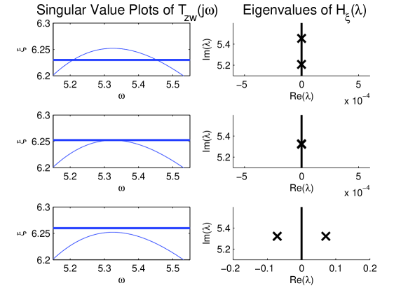
Figure 1: (left) Intersections of the singular value plot of $T_{zw}$ with the horizontal line $\xi=c$, for $c<\hat{\xi}$ (top), $c=\hat{\xi}$ (middle) and $c>\hat{\xi}$ (bottom). (right) Corresponding eigenvalues of $H_{\xi}(\lambda)$ (26).

The drawback of working directly with (28) is that an explicit expression for the determinant of $H_{\xi}$ is required. This scalar-valued conditions can be equivalently expressed in a matrix-based formulation.

$${\textstyle\left\{\begin{array}[]{l}H(j\omega,\ \xi)\left[\begin{array}[]{c}u,\\ v\end{array}\right]=0,\quad n(u,v)=0,\\ \Im\left\{v^{*}\left(I+\sum_{i=1}^{m+1}A_{cl,i}\tau_{i}e^{-j\omega\tau_{i}}\right)u\right\}=0\\ \end{array}\right.}$$ (29)

where $n(u,v)=0$ is a normalizing condition. The approximate H-infinity norm and its corresponding frequencies can be corrected by solving (29). For further details, see sg_TW551 .

2.5 Computing the Gradients

The optimization algorithm requires the derivatives of H-infinity norm of the transfer function $T_{zw}$ with respect to the controller matrices whenever it is differentiable. Define the H-infinity norm of the function $T_{zw}$ as

$$f(A_{cl,0},\ldots,A_{cl,{m+2}},B_{cl},C_{cl},D_{cl})=\|T_{zw}(j\omega)\|_{\infty}.$$

These derivatives exist whenever there is a unique frequency $\hat{\omega}$ such that (27) holds, and, in addition, the largest singular value $\hat{\xi}$ of $T_{zw}(j\hat{\omega})$ has multiplicity one. Let $w_{l}$ and $w_{r}$ be the corresponding left and right singular vector, i.e.

$${\small\begin{array}[]{l}T_{zw}(j\hat{\omega})\ w_{r}=\hat{\xi}\ w_{l},\\ w_{l}^{*}\ T_{zw}(j\hat{\omega})=\hat{\xi}\ w_{r}^{*}.\end{array}}$$ (30)

When defining $\frac{\partial f}{\partial A_{cl,0}}$ as a n-by-n matrix whose $(k,l)$-th element is the derivative of $f$ with respect to the $(k,l)$-th element of $A_{cl,0}$, and defining the other derivatives in a similar way, the following expressions are obtained sg_Marc :

$$\frac{\partial f}{\partial A_{cl,0}} = \frac{\Re\left(M(j\hat{\omega})^{*}C_{cl}^{T}w_{l}w_{r}^{*}B_{cl}^{T}M(j\hat{\omega})^{*}\right)}{w_{r}^{*}w_{r}},$$

$$\frac{\partial f}{\partial A_{cl,i}} = \frac{\Re\left(M(j\hat{\omega})^{*}C_{cl}^{T}w_{l}w_{r}^{*}B_{cl}^{T}M(j\hat{\omega})^{*}e^{j\omega\tau_{i}}\right)}{w_{r}^{*}w_{r}}\ \textrm{for}\ i=1,\ldots,m+2,$$

$$\frac{\partial f}{\partial B_{cl}} = \frac{\Re(M(j\hat{\omega})^{*}C_{cl}^{T}w_{l}w_{r}^{*})}{w_{r}^{*}w_{r}},\frac{\partial f}{\partial C_{cl}}=\frac{\Re(w_{l}w_{r}^{*}B_{cl}^{T}M(j\hat{\omega})^{*})}{w_{r}^{*}w_{r}},$$

$$\frac{\partial f}{\partial D_{cl}} = \frac{\Re\left(w_{l}w_{r}^{*}\right)}{w_{r}^{*}w_{r}}$$

where $M(j\omega)=\left(j\omega I-A_{cl,0}-\sum_{i=1}^{m+2}A_{cl,i}e^{-j\omega\tau_{i}}\right)^{-1}$.

We compute the gradients with respect to the controller matrices as

$$\frac{\partial f}{\partial A_{K}} = \left[\begin{array}[]{cc}0_{n_{K}\times n}&I_{n_{K}}\end{array}\right]\frac{\partial f}{\partial A_{cl,0}}\left[\begin{array}[]{c}0_{n\times n_{K}}\\ I_{n_{K}}\end{array}\right],$$ (34)

$$\frac{\partial f}{\partial B_{K}} = \left[\begin{array}[]{cc}0_{n_{K}\times n}&I_{n_{K}}\end{array}\right]\frac{\partial f}{\partial A_{cl,0}}\left[\begin{array}[]{c}I_{n}\\ 0_{n_{K}\times n}\end{array}\right]C_{2}^{T}$$ (43)

$$+\left[\begin{array}[]{cc}0_{n_{K}\times n}&I_{n_{K}}\end{array}\right]\frac{\partial f}{\partial A_{cl,{m+2}}}\left[\begin{array}[]{c}0_{n\times n_{K}}\\ I_{n_{K}}\end{array}\right]C_{K}^{T}D_{22}^{T}+\left[\begin{array}[]{cc}0_{n_{K}\times n}&I_{n_{K}}\end{array}\right]\frac{\partial f}{\partial B_{cl}}D_{21}^{T},$$

$$\frac{\partial f}{\partial C_{K}} = B_{2}^{T}\left[\begin{array}[]{cc}I_{n}&0_{n\times n_{K}}\end{array}\right]\frac{\partial f}{\partial A_{cl,{m+1}}}\left[\begin{array}[]{c}0_{n\times n_{K}}\\ I_{n_{K}}\end{array}\right]$$ (53)

$$+D_{22}^{T}B_{K}^{T}\left[\begin{array}[]{cc}0_{n_{K}\times n}&I_{n_{K}}\end{array}\right]\frac{\partial f}{\partial A_{cl,{m+2}}}\left[\begin{array}[]{c}0_{n\times n_{K}}\\ I_{n_{K}}\end{array}\right]+D_{12}^{T}\frac{\partial f}{\partial C_{cl}}\left[\begin{array}[]{c}0_{n\times n_{K}}\\ I_{n_{K}}\end{array}\right]$$

where the matrices $I_{n}$, $I_{n_{K}}$ and $0_{n\times n_{K}}$, $0_{n_{K}\times n}$ are identity and zero matrices.

3 Examples

We consider the time-delay system with the following state-space representation,

$$\dot{x}(t) = -x(t)-0.5x(t-1)+w(t)+u(t),$$

$$z(t) = x(t)+u(t),$$

$$y(t) = x(t)+w(t).$$

We designed the first-order controller, $n_{K}=1$,

$$\dot{x}_{K}(t) = 3.61x_{K}(t)+1.39y(t),$$

$$u(t) = -0.83x_{K}(t)$$

achieving the closed-loop H-infinity norm $0.064$. The closed-loop H-infinity norms of fixed-order controllers for $n_{K}=2$ and $n_{K}=3$ are $0.021$ and $0.020$ respectively.

Our second example is a $4^{\rm{th}}$-order time-delay system. The system contains $4$ delays and has the following state-space representation,

$$\dot{x}(t)=\left(\begin{array}[]{cccc}-4.4656&-0.4271&0.4427&-0.1854\\ -0.8601&-5.6257&0.8577&-0.5210\\ 0.9001&-0.7177&-6.5358&0.0417\\ -0.6836&0.0242&0.4997&-3.5618\end{array}\right)x(t)+\left(\begin{array}[]{cccc}0.6848&-0.0618&0.5399&0.5057\\ 0.3259&-0.3810&0.6592&-0.0066\\ 0.6325&0.3752&0.4122&0.7303\\ 0.5878&0.9737&0.1907&-0.8639\end{array}\right)x(t-3.2)\\ +\left(\begin{array}[]{cccc}0.9371&-0.7859&0.1332&0.7429\\ -0.8025&0.4483&0.6226&0.0152\\ 0.0940&0.2274&0.1536&0.5776\\ -0.1941&0.5659&0.8881&-0.0539\end{array}\right)x(t-3.4)+\left(\begin{array}[]{cccc}0.6576&-0.8543&-0.3460&0.6415\\ -0.3550&0.5024&0.6081&0.9038\\ 0.9523&0.6624&0.0765&-0.8475\\ -0.4436&0.8447&-0.0734&0.4173\\ \end{array}\right)x(t-3.9)\\ +\left(\begin{array}[]{cc}1&0\\ -1.6&1\\ 0&0\\ 0&0\end{array}\right)w(t)+\left(\begin{array}[]{cc}0.2\\ -1\\ 0.1\\ -0.4\\ \end{array}\right)u(t-0.2)$$ (54)

$$z(t) = \left(\begin{array}[]{cccc}1&0&0&-1\\ 0&-1&1&0\end{array}\right)x(t)+\left(\begin{array}[]{cc}0.1&1\\ -1&0.2\end{array}\right)w(t)+\left(\begin{array}[]{c}1\\ -1\end{array}\right)u(t)$$ (61)

$$y(t) = \left(\begin{array}[]{cccc}1&0&-1&0\end{array}\right)x(t)+\left(\begin{array}[]{cc}-2&0.1\end{array}\right)w(t)+0.4u(t-0.2)$$ (64)

When $n_{K}=1$, our method finds the controller achieving the closed-loop H-infinity norm $1.2606$,

$$\dot{x}_{K}(t) = -0.712x_{K}(t)-0.1639y(t),$$

$$u(t) = -0.2858x_{K}(t)$$

and the results for $n_{K}=2$ and $n_{K}=3$ are $1.2573$ and $1.2505$ respectively.

4 Concluding Remarks

We successfully designed fixed-order H-infinity controllers for a class of time-delay systems. The method is based on non-smooth, non-convex optimization techniques and allows the user to choose the controller order as desired. Our approach can be extended to general time-delay systems. Although we illustrated our method for a dynamic controller, it can be applied to more general controller structures. The only requirement is that the closed-loop matrices should depend smoothly on the controller parameters. On the contrary, the existing controller design methods optimizing the closed-loop H-infinity norm are based on Lyapunov theory and linear matrix inequalities, which are conservative if the form of the Lyapunov functions are restricted and requires full state information.

5 Acknowledgements

This article presents results of the Belgian Programme on Interuniversity Poles of Attraction, initiated by the Belgian State, Prime Minister s Office for Science, Technology and Culture, the Optimization in Engineering Centre OPTEC of the K.U.Leuven, and the project STRT1-09/33 of the K.U.Leuven Research Foundation.

References

• (1) A. Blomqvist, A. Lindquist and R. Nagamune (2003) Matrix-valued Nevanlinna-Pick interpolation with complexity constraint: An optimization approach. IEEE Transactions on Automatic Control, 48:2172–2190.
• (2) S. Boyd and V. Balakrishnan (1990) A regularity result for the singular values of a transfer matrix and a quadratically convergent algorithm for computing its $\mathcal{L}_{\infty}$-norm. Systems & Control Letters, 15:1–7.
• (3) D. Breda, S. Maset and R. Vermiglio (2006) Pseudospectral approximation of eigenvalues of derivative operators with non-local boundary conditions. Applied Numerical Mathematics, 56:318–331.
• (4) N.A. Bruinsma and M. Steinbuch (1990) A fast algorithm to compute the $\mathcal{H}_{\infty}$-norm of a transfer function matrix. Systems & Control Letters, 14:287–293.
• (5) J.V. Burke, D. Henrion, A.S. Lewis and M.L. Overton (2006). Stabilization via nonsmooth, nonconvex optimization. IEEE Transactions on Automatic Control, 51:1760 -1769.
• (6) J.V. Burke, A.S. Lewis and M.L. Overton, (2003) A robust gradient sampling algorithm for nonsmooth, nonconvex optimization. SIAM Journal on Optimization, 15:751–779.
• (7) R. Byers (1988) A bisection method for measuring the distance of a stable matrix to the unstable matrices. SIAM Journal on Scientific and Statistical Computing, 9:875–881.
• (8) J.C. Doyle, K. Glover, P.P. Khargonekar and B.A. Francis (1989) State-Space solutions to standard $\mathcal{H}^{2}$ and $\mathcal{H}^{\infty}$ control problems. IEEE Transactions on Automatic Control 46:1968–1972.
• (9) P. Gahinet and P. Apkarian (1994) An Linear Matrix Inequality Approach to $\mathcal{H}_{\infty}$ Control. International Journal of Robust and Nonlinear Control 4:421–448.
• (10) S. Gumussoy and M.L. Overton, (2008) Fixed-Order H-Infinity Controller Design via HIFOO, a Specialized Nonsmooth Optimization Package. Proceedings of the American Control Conference 2750 -2754.
• (11) R. Hryniv and P. Lancaster (1999) On the perturbation of analytic matrix functions. Integral Equations and Operator Theory, 34:325–338.
• (12) A.S. Lewis and M.L.Overton, (2009) Nonsmooth optimization via BFGS. Submitted to SIAM Journal on Optimization.
• (13) W. Michiels and S. Gumussoy, (2009) Computation of H-infinity Norms for Time-Delay Systems. Accepted to SIAM Journal on Matrix Analysis and Applications. See also Technical Report TW551, Department of Computer Science, K.U.Leuven, 2009.
• (14) M. Millstone, (2006) HIFOO 1.5: Structured control of linear systems with a non-trivial feedthrough. Master’s Thesis, New York University.
• (15) J. Vanbiervliet, K. Verheyden, W. Michiels and S. Vandewalle (2008) A nonsmooth optimization approach for the stabilization of time-delay systems. ESAIM Control, Optimisation and Calcalus of Variations 14:478–493.
• (16) K. Zhou, J.C. Doyle and K. Glover (1995) Robust and optimal control. Prentice Hall.
Index