Where Should You Park Your Car? The $\frac{1}{2}$ Rule

Abstract

We investigate parking in a one-dimensional lot, where cars enter at a rate $\lambda$ and each attempts to park close to a target at the origin. Parked cars also depart at rate 1. An entering driver cannot see beyond the parked cars for more desirable open spots. We analyze a class of strategies in which a driver ignores open spots beyond $\tau L$, where $\tau$ is a risk threshold and $L$ is the location of the most distant parked car, and attempts to park at the first available spot encountered closer than $\tau L$. When all drivers use this strategy, the probability to park at the best available spot is maximal when $\tau=\frac{1}{2}$, and parking at the best available spot occurs with probability $\frac{1}{4}$.

1 Introduction and Model

One of the downsides of driving to a popular destination is that good parking spaces near the venue may be hard to find. The dilemma is whether to park far away, which should be easy, and then have a long walk to the destination, or drive close to the venue and then look for a good parking spot, which is likely to be hard. In this work, we investigate a simple class of threshold-driven parking strategies in an idealized parking lot geometry. We find the strategy that maximizes the probability to park in the best available spot.

Because of its pervasive role in our daily lives, understanding parking has been the focus of much study, especially in the urban planning and transportation engineering literatures (see, e.g., [1, 2, 3, 4, 5, 6, 7] and references therein). To help in making policy decisions, these investigations typically include many real-world effects, such as practical parking-lot geometries, parking costs, parking limits, and urban planning implications. It is difficult to gain fundamental insights from such reality based approaches. Our approach is to investigate a parsimonious model that captures some key features of parking, and for which some analytic understanding can be gleaned.

For simplicity, the parking lot is one-dimensional, with parking spots labeled by the positive integers $k=1,2,\ldots$ and the desired target is located at $k=0$ (Fig. 1). Cars enter one at a time from the right at rate $\lambda$ and each car also departs at rate 1; this input rate is the only parameter of the system. The dynamics of the number of cars is governed by the Poisson process, independent of the parking strategy. However, the spatial distribution of parked cars depends on the parking strategy.

We postulate that a driver cannot see open parking spots closer to the target than the current position of the driver (if there is a contiguous gap of open spots at the current position, the driver can see only to the end of this gap). We additionally assume that after entering the lot, the driver finds a parking space before the next car enters or any of the parked cars depart. While this model is highly idealized, it captures the tradeoff involved in looking for open spots in a crowded parking lot.

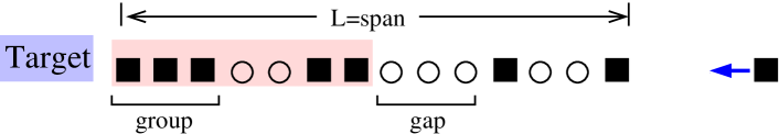
Figure 1: Parking in a one-dimensional lot where cars (squares) enter from the right and circles represent empty spots. Spots beyond the furthest car are not shown. The next car to enter (blue arrow) will start looking for a parking spot in the active zone (red shaded area). In this example, this next entering car parks a distance $k=4$ from the target, which happens to be the best available spot. Here $N=7$, $L=14$, $V=7$, and $\tau=\frac{1}{2}$.

The parked cars form groups that are interspersed by gaps (Fig. 1). Two basic macroscopic observables are the total number of parked cars $N$ and the span $L$, defined as the distance between the target and the most distant parked car. We are particularly interested in the number of open parking spots within the span (henceforth referred to as vacancies) $V=L-N$, as well as their spatial distribution. While the state of the parking lot is always changing, due to the stochastic arrival and departure of cars, the state of the lot is statistically stationary. Moreover, relative fluctuations become small in the $\lambda\to\infty$ limit. From the underlying Poisson process for the number of parked cars, $\langle N\rangle=\lambda$ and $\langle N^{2}\rangle-\langle N\rangle^{2}=\lambda$, so the relative standard deviation vanishes as $\lambda^{-1/2}$. In real life, parking lots are often nearly full, which corresponds to large $\lambda$ in our model. Hence we assume $\lambda\gg 1$ unless stated otherwise.

All drivers follow the same parking strategy and we seek the optimal strategy, which we define as the one that maximizes the probability to find the best available spot without backtracking, i.e., the vacancy closest to the target. (If backtracking occurs, the filled vacancy is closest to the target, but there is the added expense of backtracking.)  We analyze a class of threshold parking strategies that are inspired by threshold strategies that arise in a wide variety of optimal decision problems  [8, 9, 10, 11, 12]. The classic “secretary problem” [9, 10, 11, 12, 13, 14, 15, 16, 17, 18, 19, 20, 21, 22] is perhaps the best-known example of the utility of a threshold rule. In the framework of our parking problem, the threshold characterizes the degree of risk that an entering driver is willing to accept. We thus define a risk threshold $\tau\in(0,1)$ as follows: When a car enters the parking lot whose current span is $L$, the driver ignores all vacancies in $[\tau L,L)$ and only starts looking for vacancies upon reaching a distance $\tau L$ from the target. The driver parks at the end of the first eligible gap encountered that is closest to the target (Fig. 1). If no gaps are found when the target is reached, the driver backtracks and parks in the first available vacancy, whose location is necessarily greater than $\tau L$. We call the zone $(0,\tau L)$ active since drivers actively look for vacancies there; in the complementary passive zone $[\tau L,L)$, vacancies are initially ignored.

We shall show that in the $\lambda\to\infty$ limit, the probability for a driver to park in the best available spot is maximized by choosing $\tau=\frac{1}{2}$. Normally one does not park at the first vacancy encountered because one feels that better spots will be available. But waiting too long may result in the failure to find an available spot. The $\mathbf{\frac{1}{2}}$ Rule provides the best compromise between actually finding a spot and not being a sucker for parking too far away. For the $\tau$-threshold strategy, we will show that the probability to find a single vacancy in the active zone, which is the same as finding the best available parking spot, is $P_{1}(\tau)=\tau(1-\tau)$. This probability is maximized when $\tau=\frac{1}{2}$ and the maximum value of $P_{1}(\tau)$ equals $\frac{1}{4}$.

We previously studied parking in the same one-dimensional geometry [23], in which parking occurred according to either the optimistic strategy or to the prudent strategy. In the optimistic strategy, the driver goes all the way to the target and then backtracks to the closest available spot. In the prudent strategy, the driver parks at the first gap encountered; when there are no vacancies, the driver backtracks and parks behind the rightmost parked car. These two rules correspond to the risk threshold $\tau=0$ and $\tau=1$, respectively. We will see that these two extremal parking rules are both inferior to the strategy with $\tau=\frac{1}{2}$.

In the next section, we present simulation data for the spatial distribution of cars and the complementary distribution of vacancies. The latter distribution has a rich spatial structure and we offer conjectures for the vacancy density in the active and passive zones that appear to be exact. In Sect. 3 we derive the distribution of the number of vacancies $P_{n}(\tau)$ in the active zone. In Sect. 4 we argue that the position of the chosen parking spot is spatially uniform, independent of the threshold $\tau$. In Sect. 5 we determine the cost associated with parking and the parking strategy that minimizes this cost. Finally, in Sect. 6 we summarize our results and give some perspectives.

2 Spatial Distributions of Parked Cars and Vacancies

For the threshold rule with $\tau$ strictly less than 1, the average density of parked cars at position $k$ approaches a step function as the arrival rate $\lambda\to\infty$: $\rho(k)=1$ for $k<\lambda$ and $\rho(k)=0$ for $k>\lambda$ (Fig. 2(a)). That is, the bulk of the parking lot is full and most vacancies are near the far end of the lot where $k\approx\lambda$. Figure 2(b) shows the density profile near the top of the “Fermi sea” plotted versus the appropriate ‘boundary-layer’ variable $\xi=(k-\lambda)/\lambda^{1/2}$. The deviation of the spatial distribution from a step function vanishes as $\lambda^{-1/2}$ for $\lambda\to\infty$ and the data for other values of $\tau$ are qualitatively similar.

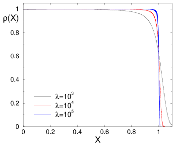
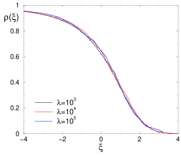
Figure 2: (a) Simulation data for the density profile of parked cars versus $X=k/\lambda$. (b) The density profile in the front region versus the boundary-layer variable $\xi=(X-1)\lambda^{1/2}$. In (b), the data for $\lambda=10^{4}$ and $\lambda=10^{5}$ are smoothed over 10-point and 100-point ranges, respectively. For both plots $\tau=\frac{1}{2}$.

Because the lot is nearly full for large $\lambda$, it is more revealing to focus on the spatial distribution of vacancies $1-\rho(k)$. Since the vacancy density is of the order of $1/\lambda$ in the nearly fully occupied region of the parking lot, it is useful to define the scaled location $X\equiv k/\lambda$ and the scaled vacancy density

$$N(X)=\lambda[1-\rho(k)]\,.$$ (1)

With this rescaling, we numerically observe that the vacancy density $N_{a}(X)$ in the active zone (defined by $X<\tau$ in scaled units) is well fit by the simple form (Fig. 3(a)):

$$N_{a}(X)=\frac{1}{(X+1-\tau)^{2}}\qquad\qquad 0\leq X\leq\tau\,.$$ (2)

This conjectured form of the density profile implies that the average number of vacancies in the active zone is

$$\langle n\rangle_{a}=\int_{0}^{\tau}dX\,N_{a}(X)=\frac{\tau}{1-\tau}\,.$$ (3)

This result turns out to be asymptotically exact, and we derive it in the next section without relying on (2).

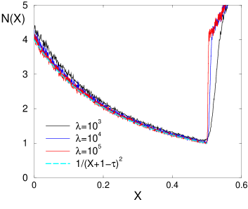
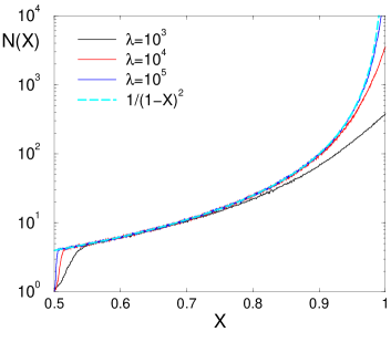
Figure 3: The scaled density profile of vacancies for $\tau=\frac{1}{2}$ in: (a) the active zone $X<\frac{1}{2}$, and (b) the passive zone $X>\frac{1}{2}$. The data for $\lambda=10^{4}$ and $\lambda=10^{5}$ are smoothed over a 10-point and 100-point range, respectively.

If there are no vacancies in the active zone, the driver must backtrack and park in the passive zone. Qualitatively, the parking mechanism in the passive zone is the mirror image of parking in the active zone. Based on this insight, as well as on the numerical data itself, we make the guess that the scaled vacancy density in the passive zone $\tau<X<1$ is given by

$$N_{p}(X)=\frac{1}{(1-X)^{2}}\qquad\qquad\tau<X<1\,.$$ (4)

This simple form also provides an excellent fit to the data in the spatial portion of the parking lot that is nearly full (Fig. 3(b)).

The jump in the vacancy density profile at $X=\tau$ reflects the nature of the threshold strategy. Since a driver starts looking for a vacancy only when $X=\tau$ is reached, parking spots just closer than $X=\tau$ are likely to be taken, while the best spots close to $X=0$ are likely to be “wasted”. Conversely, if one needs to backtrack to park, it is the spots just beyond $X=\tau$ that will be taken, while more distant parking spots will remain more plentiful. A curious and unexplained feature of the density profiles (2) and (4) is that $N_{a}(X=0)=N_{p}(X=\tau)$.

From the density (4), we estimate the number of vacancies in the passive zone by

$$\langle n\rangle_{p}=\int_{\tau}^{1-\epsilon}dX\,N_{p}(X)\,.$$ (5)

Here, we introduce an upper cutoff to the integral because the vacancy density (4) cannot hold all the way to $X=1$. Since the density profile has a transition zone whose width is of the order of $\lambda^{1/2}$, the cutoff in scaled units should be $\epsilon\sim\lambda^{-1/2}$. With this cutoff, (5) gives $\langle n\rangle_{p}\sim\lambda^{1/2}$. Thus for large $\lambda$ and with drivers all following the same threshold strategy, there are of the order of $\lambda^{1/2}$ lousy parking spots more distant than the threshold, and a few good parking spots within the threshold.

3 Number of Vacancies in the Active Zone

We now derive the distribution of the number of vacancies in the active zone, from which we deduce the optimality of the $\frac{1}{2}$ rule. Denote by $P_{n}(\tau)$ the probability to find $n$ vacancies in the active zone of the parking lot, $0<X<\tau$, when the threshold is $\tau$. Further, define $V_{1}(X_{1};\tau)$ as the probability density for a single vacancy at $X_{1}$ and generally $V_{n}(X_{1},\ldots,X_{n};\tau)$ as the probability density for $n$ vacancies at $0<X_{1}<X_{2}<\ldots<X_{n}<\tau$. The probability to find $n$ vacancies in the active zone is therefore

$$P_{n}=\int\cdots\int_{0<X_{1}<\ldots<X_{n}<\tau}dX_{1}\ldots dX_{n}\,V_{n}(X_{1},\ldots,X_{n};\tau)\,.$$ (6)

Hereinafter we typically drop the dependence on $\tau$ to declutter the notation. Explicitly

$$P_{1} =\int_{0}^{\tau}dX_{1}\,\,V_{1}(X_{1})\,,$$ (7a)

$$P_{2} =\int_{0}^{\tau}dX_{1}\int_{X_{1}}^{\tau}dX_{2}\,\,V_{2}(X_{1},X_{2})\,,$$ (7b)

$$P_{3} =\int_{0}^{\tau}dX_{1}\int_{X_{1}}^{\tau}dX_{2}\int_{X_{2}}^{\tau}dX_{3}\,\,V_{3}(X_{1},X_{2},X_{3})\,,$$ (7c)

etc. For notational consistency, we also write $V_{0}=P_{0}$ for the probability of no vacancies in the active zone.

To compute the probability distribution $P_{n}$ for the number of vacancies in the active zone, we ostensibly need the densities $V_{n}$. As we now show, our approach circumvents the need for the complete information about these densities. The quantity $V_{0}$ satisfies the rate equation

$$\frac{dV_{0}}{dt}=-\lambda\tau V_{0}+\lambda\int_{0}^{\tau}dX_{1}\,V_{1}(X_{1})\,.$$ (8)

The loss term on the right accounts for the departure of a car from the fully occupied active zone. The gain term accounts for a car that parks in the single vacancy within the active zone. In the steady state, (8) becomes

$$\int_{0}^{\tau}dX_{1}\,V_{1}(X_{1})=\tau V_{0}\,.$$ (9)

The left-hand side of (9) equals $P_{1}$ (see (7a)), so we have

$$P_{1}=\tau V_{0}\,.$$ (10)

Similarly to (8), we write the rate equation for $V_{1}(X_{1})$. In the steady state, this equation reduces to

$$\int_{X_{1}}^{\tau}dX_{2}\,V_{2}(X_{1},X_{2})+V_{0}=\tau V_{1}(X_{1})+V_{1}(X_{1})\,.$$ (11)

The first term on the left side accounts for parking when two vacancies exist, while the second term accounts for the departure of a car from the fully occupied active zone. The first term on the right accounts for the departure of a car when the active zone contains a single vacancy, while the second term accounts for a car that parks at $X_{1}$. We now integrate (11) over the active zone, $0<X_{1}<\tau$. Using (7b), the left-hand side becomes $P_{2}+\tau V_{0}$, while the right-hand side becomes $(1+\tau)P_{1}$, after recalling (7a). Hence $P_{2}=(1+\tau)P_{1}-\tau V_{0}$, which, in conjunction with (10), yields

$$P_{2}=\tau^{2}V_{0}\,.$$ (12)

Continuing this line of reasoning, we write the rate equation for $V_{2}(X_{1},X_{2})$. In the steady state, this equation reduces to

$$(\tau+1)V_{2}(X_{1},X_{2}) =\int_{X_{2}}^{\tau}dX_{3}\,V_{3}(X_{1},X_{2},X_{3})+V_{1}(X_{1})+V_{1}(X_{2})\,.$$ (13)

Integrating (13) over $0<X_{1}<X_{2}<\tau$ ultimately yields

$$P_{3}=\tau^{3}V_{0}\,.$$ (14)

Following this approach for general $n$, we find $P_{n}=\tau^{n}V_{0}$. The normalization condition, $\sum_{n\geq 0}P_{n}=1$, fixes $V_{0}$ to be $1-\tau$. Thus the distribution of the number of vacancies in the active zone is the geometric distribution

$$P_{n}(\tau)=(1-\tau)\tau^{n}\,.$$ (15)

The average number of vacancies in the active zone, $0<X<\tau$, is therefore

$$\langle n\rangle_{a}=\sum_{n\geq 0}nP_{n}(\tau)=\frac{\tau}{1-\tau}\,.$$ (16)

Our simulation data in Fig. 4 is in excellent agreement with the prediction (15).

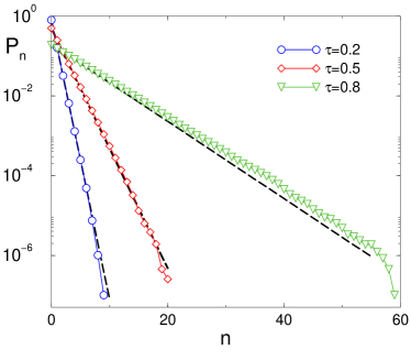
Figure 4: The probability $P_{n}$ for $n$ vacancies in the active zone for three threshold values and for $\lambda=10^{4}$. The dashed lines are the theoretical predictions from (15).

From (15), the probability to have one vacancy in the active zone is $P_{1}(\tau)=\tau(1-\tau)$. By its definition, this quantity coincides with the probability that a newly entering car parks in the best available spot. This probability is maximized when $\tau=\tau_{*}=\frac{1}{2}$. At this optimal threshold value, there is one vacancy, on average, in the active zone and the probability of actually parking in the best available spot is $P_{1}(\tau_{*})=\frac{1}{4}$.

4 The Best and the Actual Parking Spot

A natural question that arises upon entering a crowded parking lot is: where is the best open parking spot? Let $B(X)$ be the probability density to have the best parking spot at $X$. This probability density has a non-trivial spatial structure (Fig. 5). For $\tau=0$ (the optimistic strategy in Ref. [23]), the distribution is flat: $B(X)=1$. That is, if one drives straight to the target and then starts looking for a parking spot by backtracking, the closest parking spot is equiprobably anywhere in the lot.

For the general situation, $0<\tau<1$, the distribution $B(X)$ exhibits different behaviors in the active and passive zones, with a jump at $X=\tau$. In the passive zone, which gets occupied due to backtracking, the distribution is again flat; moreover, $B_{p}(X)=1$ for $X>\tau$. In the active zone, $X<\tau$, the probability density $B_{a}(X)$ is a decreasing function of $X$ which becomes progressively more peaked as $\tau$ increases. That is, if one starts looking for parking spots when $X$ reaches $\tau$, it is the parking spots with $X\mathrel{\raise 1.29167pt\hbox{$<$\kern-7.5pt\lower 4.30554pt\hbox{$\sim$}}}\tau$ that are more likely to be filled, while the desirable spots near $X=0$ will be relatively unfilled. The probability density to have the best spot next to the target, $B_{a}(0)$, is obviously equal to the vacancy density $N_{a}(0)$; this implies that $B_{a}(0)=(1-\tau)^{-2}$. The probability density $B(X)$ is normalized, so that $\int_{0}^{\tau}dX\,B_{a}(X)=\tau$. These are two exact properties of the probability density $B_{a}(X)$ in the active zone. The challenge is to determine $B_{a}(X)$ analytically.

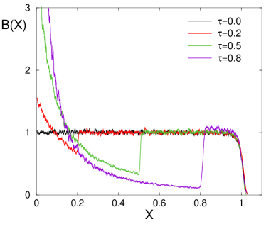
Figure 5: The probability density $B(X)$ that the best parking spot is at a scaled distance $X$ from the target for threshold strategies with $\tau=0,~{}0.2,~{}0.5,~{}0.8$. The data are based on $\lambda=10^{4}$ and are smoothed over a 50-point range.

The threshold-$\frac{1}{2}$ rule leads to success, viz., to parking in the best available spot, in a fraction $P_{1}(\frac{1}{2})=\frac{1}{4}$ of attempts; otherwise parking occurs in a suboptimal spot. Thus a useful measure of the efficacy of the threshold strategy is the ratio $r\equiv X/X_{B}$ of the actual parking location $X$ to the best available location $X_{B}$. Denote by $q(r)$ the probability density that $X/X_{B}=r$. We know that $r=1$ if there is either 1 or 0 vacancies in the active zone. In these two cases, the car parks in the best available spot without backtracking or with backtracking, respectively. The two events occur with probability $P_{0}+P_{1}=1-\tau^{2}$. Hence

$$q(r)=(1-\tau^{2})\delta(r-1)+Q(r).$$ (17)

The continuous part $Q(r)$ of the probability density accounts for the situations when there is more than one vacancy in the active zone, so the entering car necessarily parks in a suboptimal spot and $r>1$.

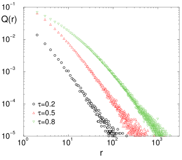
Figure 6: The continuous part $Q(r)$ of the probability density of the ratio of the actual parking location to the best parking location, $r=X/X_{B}$.

The continuous part $Q(r)$ of the probability density satisfies $\int_{1}^{\infty}dr\,Q(r)=\tau^{2}$ and it appears to have a power-law tail for large $r$ (Fig. 6) in the general situation when $0<\tau<1$. For the threshold values shown in this figure, the data is reasonably fit by the power law $r^{-\nu}$, with $\nu\approx 1.8$. That is, even though a driver typically does not park in the best spot, it is likely that parking occurs close to the best spot. When $\tau=0$ (the optimistic strategy in [23]), the car necessarily parks in the best spot by backtracking: $q(r)=\delta(r-1)$.

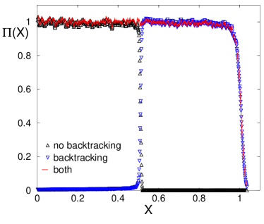
Figure 7: The spatial distribution of parking locations for $\tau=\frac{1}{2}$. The data have been smoothed over a 50-point range and only every tenth data point is shown.

Although the ratio of the actual parking location to the best location has a non-trivial distribution, the spatial distribution of the actual parking location $\Pi(X)$ is remarkably simple: $\Pi(X)=1$ (Fig. 7). To understand this striking result, consider the part of this distribution $\Pi_{a}(X)$ in the active zone, $X\leq\tau$, when a car finds a parking spot without backtracking. The strategy in the active zone is effectively the same as the strategy with an effective threshold $\tau_{\text{eff}}=1$ in the case where the span is $\tau L$. The properly scaled spatial variable is $X/\tau$ and hence

$$\Pi_{a}(X)=\Phi(y),\quad y=\frac{X}{\tau}\,.$$ (18a)

When backtracking occurs, cars enter the passive zone and park in the first gap, so effectively they follow the prudent strategy with span $(1-\tau)L$. The properly scaled spatial variable is now $(1-X)/(1-\tau)$ as the cars move to right when they backtrack. Thus the part of the parking distribution $\Pi_{p}(X)$ that corresponds to the passive zone is

$$\Pi_{p}(X)=\Phi(y),\quad y=\frac{1-X}{1-\tau}\,.$$ (18b)

The fractions of cars that park in the active and passive zones are $\tau$ and $1-\tau$. These fractions also equal $\int_{0}^{\tau}dX\,\Pi_{a}(X)$ and $\int_{\tau}^{1}dX\,\Pi_{p}(X)$, respectively. Using (18a)–(18b) we indeed recover $\tau$ and $1-\tau$ after imposing the normalization condition

$$\int_{0}^{1}dy\,\Phi(y)=1\,.$$ (19)

To determine the form of the probability density $\Pi(X)$, let us compute its derivatives at the threshold location $X=\tau$:

$$\frac{d^{n}\Pi}{dX^{n}}\Big{|}_{X=\tau-0} =\tau^{-n}\Phi^{(n)}(1)\,,$$

$$\frac{d^{n}\Pi}{dX^{n}}\Big{|}_{X=\tau+0} =(-1)^{n}(1-\tau)^{-n}\Phi^{(n)}(1)\,,$$

where $\Phi^{(n)}(y)=d^{n}\Phi(y)/dy^{n}$. The derivatives from left and write coincide only if $\Phi^{(n)}(1)=0$ for all $n\geq 1$. Thus $\Pi(X)$ is smooth at $X=\tau$ when all derivatives of $\Phi(y)$ vanish at $y=1$. The vanishing of all derivatives implies that the distribution is uniform, and the actual value $\Phi(y)=1$ is fixed by the normalization condition (19). Our above argument is not a proof, but it shows that postulating analyticity of the probability density $\Pi(X)$ at the threshold $X=\tau$ suffices to derive its uniformity.

5 Cost of Parking

Maximizing the probability to park in the best available spot is natural and may be compatible with the intrinsic irrationality of human behavior in parking lots (see, e.g., [24]). However, the threshold parking rule is not necessarily the most rational. A more logical approach is to minimize the cost of parking, which we define as the arrival time to reach the target. This arrival time is the sum of the time spent in driving in the lot to find the parking spot plus the walking time from the parking spot to the target. In appropriate units where the walking speed equals 1, the walking time is just the distance from the parking spot to the target, while the driving time is the driving distance in the lot divided by the driving speed. This driving time also equals the driving distance multiplied by the ratio of the walking speed to the driving speed in the lot; we denote this ratio by $\epsilon$.

For the $\tau$-threshold parking strategy, these arrival times are

$$\frac{\tau}{2}+\epsilon\left(1-\frac{\tau}{2}\right)\qquad\text{and}\qquad\frac{1+\tau}{2}+\epsilon\left(1+\frac{1+\tau}{2}\right)\,,$$

for the cases of parking in the active and passive zones, respectively. Here we have made use of the result that the parking location is uniformly distributed in both the active and passive zones. Multiplying these arrival times by the probabilities for these two types of parking events, $\tau$ and $1-\tau$ respectively, the average parking cost is

$$\tfrac{1}{2}(1+3\epsilon)-\epsilon\tau^{2}\,.$$ (20)

This cost function attains a minimum with the prudent strategy, $\tau=1$. Despite being optimal according to the above choice for the cost function, the prudent strategy is psychologically upsetting to most people. In the prudent strategy, the parking spot that a driver takes is essentially never the best available, as the typical number of vacancies is of order $\sqrt{\lambda}$. Perhaps even more upsetting to a driver who has just parked is that the absolutely best parking spot—the one that is adjacent to the target—will be available in approximately $89\%$ of all realizations [23].

In deriving (20), we tacitly assumed that $\epsilon>0$; however, the limiting case of $\epsilon=0$ is actually quite natural. Setting $\epsilon=0$ is equivalent to only counting the time spent in walking to the target in the cost of parking. Since moving in a car requires little physical effort, drivers with limited walking ability, as well as drivers with little children, may find this cost function more suitable. Furthermore, if the target is a store were the drivers tend to buy heavy goods, it is again reasonable to minimize the time of walking from the target to the parked car, i.e., set $\epsilon=0$. In this case, the average parking cost is independent of strategy. Since the $\frac{1}{2}$ rule maximizes the probability of snagging the best parking spot, which everyone prefers, it is rational to adopt the threshold-$\frac{1}{2}$ rule if the cost of walking through the parking lot is prohibitively high.

6 Discussion

We investigated a class of threshold parking strategies in which a driver who enters a parking lot ignores all open spots a distance greater than $\tau L$ from the target. Starting at a distance $\tau L$, which defines the end of the active zone, the driver parks at near end of the first gap encountered. Here $L$ is the distance from the target to the last parked car and $\tau$ is the risk threshold. If there are no available spots in the desirable active zone, the driver backtracks and parks in the first spot encountered by backtracking.

When the ratio of the arrival rate to departure rate of each car is large, $\lambda\gg 1$, open parking spots are rare in the active zone, and the spots that do exist are more likely to be close to the target (Fig. 2(b)). Our primary result is that the probability for a newly entering car to park at the best available spot is maximized for $\tau=\frac{1}{2}$. At this optimal threshold, the probability of parking in this best spot is $\frac{1}{4}$. We conjecture that our strategy is the best amongst all (deterministic), and not necessarily threshold parking strategies. Proving or refuting this conjecture represents an appealing challenge.

Our analysis for number of vacancies in the active zone (Sect. 3) tacitly assumed that $0<\tau<1$; however, our main result (15) can be continued to $\tau=0$ and $\tau=1$; these limits correspond to the optimistic and prudent strategies in our earlier study [23]. This continuation correctly predicts that, for the optimistic strategy, the probability of finding the best spot without backtracking vanishes. Indeed, for this strategy, backtracking occurs with probability $\lambda/(1+\lambda)$ [23], so backtracking is asymptotically certain in this case. For the prudent strategy, the probability of backtracking vanishes as $\lambda^{-1}$, but the probability that the spot where the car actually parks is closest to the target vanishes as $\lambda^{-1/2}$. Thus the $\frac{1}{2}$ rule is superior to both the optimistic and prudent strategies in finding the best available parking spot.

While we found an optimal parking strategy, we were unable to analytically determine several natural spatial properties of the parked cars, such as the distribution of the number of vacancies $V$, the number of gaps (Fig. 1), the distribution of the span $L$, and multisite densities, such as $V_{n}(X_{1},\ldots,X_{n})$ in the active zone. Additionally, the expressions (2) and (4) for the vacancy densities in the active and passive zones, which appear to be correct, are conjectural. The decoupling approximation, which we employed in [23] to determine the average density of cars (or vacancies) at a given spatial location, fails for the threshold strategy and another analytical approach is needed.

Our threshold parking rules are inspired by the strategies that arise in optimal stopping problems and in decision theory (see, e.g., [8, 9, 10, 11, 12]). Some of the methods developed in this body of work, particularly in the realm of the famous “secretary problem” [9, 10, 11, 12, 13, 14, 15, 16, 17, 18, 19, 20, 21, 22], may prove useful to analyze optimal parking. Indeed, the best strategy for various decision theory optimization problems is often a threshold strategy [8, 13].

An intriguing contribution to the work on optimal stopping problems is the odds algorithm [17], which is summarized by adage: sum the odds to one and stop. The odds algorithm has been proved for some optimal stopping problems with independent events [17, 18, 19]. We now show that the odds algorithm holds in our case where parking events are not independent. By definition, the odds are the ratios $p/(1-p)$ where the $p$’s are the probabilities of success. In our situation, the probability of successful parking at spot $k$ is the probability $1-\rho(k)$ that this spot is empty . Since the $\rho(k)$ are very close to 1 in the bulk of the span, the odds coincide with the probabilities (i.e., the vacancy densities) to leading order. Summing the vacancy densities in the active zone yields the average number of vacancies, $\langle n\rangle_{a}=\tau/(1-\tau)$. Equating this number to one recovers the $\frac{1}{2}$ rule.

It is worth pointing out that our model assumes a homogeneous population of drivers; namely, they all have the same parking threshold parameter $\tau$. Rich behaviors may emerge for heterogeneous populations. The simplest heterogeneous population consists of drivers that each have independent random parking thresholds that, for example, are uniformly distributed on $(0,1)$. There is no longer an optimization problem to be solved, but the spatial properties of the parked cars could be interesting and tractable.

This heterogeneous model is a sort of equilibrium counterpart of the hashing problem that was originally introduced by Konheim and Weiss [25] and described by Knuth [26] using the parking problem language. This hashing problem and its numerous extensions have been subsequently studied by many authors, see, e.g., [27, 28, 29, 30, 31] and references therein. In the standard application of the hashing problem, one attempts to write a fixed-size file onto a computer disk. A random location on the disk is picked and if the file can be accommodate there, the file is written. If not, the next location is selected. If this location is empty, the file is written there. If not, continue moving in one direction until a vacancy is encountered. The list of starting locations is the hash table. In the language of parking, the lot is finite, there is no departure mechanism (files are not erased), so eventually the parking lot becomes full. Richer behaviors arise when the file sizes are variable. The correspondence between hashing and parking offers the possibility that the substantial research literature on the hashing problem could guide developments in our parking problem.

PLK thanks the hospitality of the Santa Fe Institute where this work was initiated. SR gratefully acknowledges financial support from NSF grant DMR-1608211. We also thank John Miller for helpful conversations.

References

- [1] D. Van Der Groot, A model to describe the choice of parking places, Transportation Res. Part A: Policy and Practice 16, 109 (1982).
- [2] W. Young, R. G. Thompson, and M. A. P. Taylor, A review of urban car parking models, Transport Rev. 11, 63 (1991).
- [3] K. W. Axhausen and J. W. Polak, Choice of parking: Stated preference approach, Transportation 18, 59 (1991).
- [4] R. G. Thompson and A. J. Richardson, A parking search model, Transportation Res. Part A: Policy and Practice, 32, 159 (1998).
- [5] R. Arnott and J. Rowse, Modeling Parking, J. Urban Economics 45, 97 (1999)
- [6] D. Teodorović and P. Luc̆ić, Intelligent parking systems, Eur. J. Oper. Res. 175, 1666 (2006).
- [7] A. Klappenecker, H. Lee, and J. L. Welch, Finding available parking spaces made easy, Ad Hoc Networks 12, 243 (2014).
- [8] D.V. Lindley, Dynamic programming and decision theory, J. Royal Statist. Soc. 10, 39 (1961).
- [9] M. H. DeGroot, Optimal Statistical Decisions (McGraw-Hill, New York, 1970).
- [10] Y. S. Chow, H. Robbins and D. Siegmund, Great Expectations: The Theory of Optimal Stopping (Houghton Mifflin Company, Boston, 1971).
- [11] B. A. Berezovsky and A. V. Gnedin, Problems of Best Choice (Akademia Nauk, Moscow, Russia, 1984).
- [12] J. Preater, The best-choice problem for partially ordered objects, Oper. Research Lett. 25, 187 (1999).
- [13] E. Dynkin, The optimum choice of the instant for stopping a Markov process, Sov. Math. Dokl. 4, 627 (1963).
- [14] Y. S. Chow, S. Moriguti, H. Robbins, and S. M. Samuels, Optimal selection based on relative rank (the “secretary problem”), Israel J. Math. 2, 81 (1964).
- [15] J. P. Gilbert and F. Mosteller, Recognizing the maximum of a sequence, J. Amer. Statist. Assoc. 61, 35 (1966).
- [16] T. S. Ferguson, Who solved the secretary problem?, Statist. Sci. 4, 282 (1989).
- [17] F. T. Bruss, Sum the odds to one and stop, Ann. Probab. 28, 1384 (2000).
- [18] F. T. Bruss, A note on bounds for the odds theorem of optimal stopping, Ann. Probab. 31, 1859 (2003).
- [19] R. Dendievel, New developments of the odds theorem, Math. Scientist 38, 111 (2013).
- [20] N. Georgiou, M. Kuchta, M. Morayne, and J. Niemiec, On a universal best choice algorithm for partially ordered sets, Random Struct. Alg. 32, 263 (2008).
- [21] R. Freij and J. Wästlund, Partially ordered secretaries, Elect. Commun. Probab. 15, 504 (2010).
- [22] B. Garrod and R. Morris, The secretary problem on an unknown poset, Random Struct. Alg. 43, 429 (2013).
- [23] P. L. Krapivsky and S. Redner, Simple parking strategies, J. Stat. Mech. 093404 (2019); arXiv:1904.06612.
- [24] T. Vanderbilt, Traffic: Why we drive the way we do (and what it says about us) (New York: Knopf, 2008).
- [25] A. G. Konheim and B. Weiss, An occupancy discipline and applications, SIAM J. Appl. Math. 14, 1266 (1966).
- [26] D. E. Knuth, The Art of Computer Programming, vol. 3, Sorting and Searching (Addison-Wesley, Reading, MA, 1973).
- [27] P. Flajolet, P. Poblete, and A. Viola, On the analysis of linear probing hashing, Algorithmica 22, 490 (1998).
- [28] S. Janson, Asymptotic distribution for the cost of linear probing hashing, Rand. Struct. Alg. 19, 438 (2001).
- [29] S. Janson, Individual displacements for linear probing hashing with different insertion policies, ACM Trans. Alg. 1, 177 (2005).
- [30] P. Flajolet and R. Sedgewick, Analytic Combinatorics (Cambridge University Press, Cambridge, UK, 2009).
- [31] M.-L. Lackner and A. Panholzer, Parking functions for mappings, J. Combin. Theor. A 142, 1 (2016).