Resilient Distributed Diffusion in Networks with Adversaries

Abstract

In this paper, we study resilient distributed diffusion for multi-task estimation in the presence of adversaries where networked agents must estimate distinct but correlated states of interest by processing streaming data. We show that in general diffusion strategies are not resilient to malicious agents that do not adhere to the diffusion-based information processing rules. In particular, by exploiting the adaptive weights used for diffusing information, we develop time-dependent attack models that drive normal agents to converge to states selected by the attacker. We show that an attacker that has complete knowledge of the system can always drive its targeted agents to its desired estimates. Moreover, an attacker that does not have complete knowledge of the system including streaming data of targeted agents or the parameters they use in diffusion algorithms, can still be successful in deploying an attack by approximating the needed information. The attack models can be used for both stationary and non-stationary state estimation. In addition, we present and analyze a resilient distributed diffusion algorithm that is resilient to any data falsification attack in which the number of compromised agents in the local neighborhood of a normal agent is bounded. The proposed algorithm guarantees that all normal agents converge to their true target states if appropriate parameters are selected. We also analyze trade-off between the resilience of distributed diffusion and its performance in terms of steady-state mean-square-deviation (MSD) from the correct estimates. Finally, we evaluate the proposed attack models and resilient distributed diffusion algorithm using stationary and non-stationary multi-target localization.

I Introduction

Diffusion Least-Mean Squares (DLMS) is a powerful algorithm for distributed state estimation [2]. It enables networked agents to interact with neighbors to process streaming data and diffuse information across the network to perform the estimation tasks. Compared to a centralized approach, distributed diffusion offers multiple advantages including robustness to drifts in the statistical properties of the data, scalability, reliance on local data, and fast response among others. Applications of distributed diffusion include spectrum sensing in cognitive networks [3], target localization [4], distributed clustering [5], and biologically inspired designs for mobile networks [6].

Diffusion strategies are known to be robust to node and link failures as well as to high noise levels [7, 8, 9, 10]. However, it is possible that a single adversarial agent that does not update its estimates according to the diffusion-based information processing rules, for instance by retaining a fixed value throughout, can fail other agents to converge to their true estimates. Resilience of diffusion-based distributed algorithms in the presence of such fixed-value Byzantine attacks has been studied in [2, 5]. A general approach to counteract such attacks is to allow agents to fuse information collected from other agents in local neighborhoods using adaptive weights instead of fixed ones. By doing so, only neighbors estimating a similar state will be assigned large weights so as to eliminate the influence of a fixed-value Byzantine adversary.

In this paper, we consider distributed diffusion for multi-task estimation where networked agents must estimate distinct, but correlated states of interest by processing streaming data. Agents use adaptive weights when diffusing information with neighbors since adaptive weights have been successfully applied to multi-task distributed estimation problems. However, we are interested in understanding if adaptive weights introduce vulnerabilities that can be exploited by Byzantine adversaries. The first problem we consider is to analyze if it is possible for an attacker to compromise a node, and make other nodes in its neighborhood converge to a state selected by the attacker. Then, we consider a network attack and determine a minimum set of nodes to compromise to make all nodes within the network converge to attacker’s desired state.

We assume a strong attack model, that is, the attacker has complete knowledge of the network topology, streaming data of targeted agents and their parameters used in the diffusion algorithm. A strong attacker can know the topology by monitoring the network, streaming data of agents by stealthily compromising their sensors/controllers and establishing backdoor channels, and diffusion parameters by doing reverse engineering. We note that having complete knowledge is a strong assumption, however, it is common to assume a strong attacker with complete knowledge of the system to examine the resilience of distributed networks [11, 12, 13, 14, 15]. In addition to this strong attack model, we also consider a weak attack model in which the attacker has no knowledge of streaming data of targeted agents or their parameters. We show that such an attacker can also be successful in preventing normal agents from converging to true estimates by approximating their states.

As a result, we show that DLMS, which was considered to be resilient against Byzantine agents by itself ([2, 5, 8]), is in fact, not resilient. A Byzantine agent sharing incorrect estimates whose values are not fixed and change over time (time-dependent Byzantine attack) can manipulate the normal agents to converge to incorrect estimates. On the one hand, adaptive weights improve the resilience of diffusion algorithms to fixed-value Byzantine attacks, but on the other hand, introduce vulnerabilities that can be exploited by time-dependent attacks. We analyze this issue in detail and propose a resilient diffusion algorithm that ensures that normal agents converge to true final estimates in the presence of any data falsification attack. The main contributions of the paper are summarized below:

$\bullet$ By exploiting the adaptive weights, we develop attack models that drive normal agents to converge to states selected by an attacker. The attack models can be used to deceive a specific node or the entire network and are applicable to both stationary and non-stationary state estimation. Although the attack models are based on a strong knowledge of the system, we also show that the attack can succeed without such knowledge.

$\bullet$ We propose a resilient distributed diffusion algorithm parameterized by a positive integer $F$. We show that if there are at most $F$ compromised agents in the neighborhood of a normal agent, then the algorithm guarantees that normal agents converge to their actual goal states under any data falsification attack. If the parameter $F$ selected by the normal agents is large, the resilient distributed diffusion algorithm degenerates to non-cooperative estimation. Thus, we also analyze trade-off between the resilience of distributed diffusion and its performance degradation in terms of the steady-state MSD.

$\bullet$ We evaluate the proposed attack models for both strong and weak attacks and the resilient distributed diffusion algorithm using both stationary and non-stationary multi-target localization. The simulation results are consistent with our theoretical analysis and show that the approach provides resilience to attacks while incurring performance degradation which depends on the assumption about the number of compromised agents.

The rest of the paper is organized as follows: Section II briefly introduces distributed diffusion. Section III presents the attack and resilient distributed diffusion problems. Sections IV and V discuss single node attack and network attack models respectively. Section VI presents and analyzes the resilient distributed diffusion algorithm. Section VII provides simulation results evaluating our approaches with multi-target localization. Section VIII discusses and evaluates the attack model that does not require complete knowledge of the system. Section IX gives a brief overview of the related work and Section X concludes the paper.

II Preliminaries

We use normal and boldface fonts to denote deterministic and random variables respectively. The superscript $(\cdot)^{*}$ denotes complex conjugation for scalars and complex-conjugate transposition for matrices, $\mathbb{E}\{\cdot\}$ denotes expectation, and $\|\cdot\|$ denotes the Euclidean norm of a vector.

Consider a network of $N$ (static) agents, in which an undirected edge (or a link) between two agents indicates that they share information and are neighbors of each other. The neighborhood of an agent $k$, denoted by $\mathcal{N}_{k}$ is the set of neighbors of $k$, including the agent $k$ itself. At each iteration $i$, agent $k$ has access to a scalar measurement $\bm{d}_{k}(i)$ and a regression vector $\bm{u}_{k,i}$ of size $M$ with zero-mean and uniform covariance matrix $R_{u,k}\triangleq\mathbb{E}\{\bm{u}_{k,i}^{*}\bm{u}_{k,i}\}>0$, which are related via a linear model of the following form:

$$\bm{d}_{k}(i)=\bm{u}_{k,i}w_{k}^{0}+\bm{v}_{k}(i).$$

where $\bm{v}_{k}(i)$ represents a zero-mean i.i.d. additive noise with variance $\sigma^{2}_{v,k}$ and $w_{k}^{0}$ denotes the unknown $M\times 1$ state vector of agent $k$.

The objective of each agent is to estimate $w_{k}^{0}$ from (streaming) data $\{\bm{d}_{k}(i),\bm{u}_{k,i}\}$ $(k=1,2,...,N,i\geq 0)$. The objective state can be static or dynamic and we represent it as $w_{k}^{0}$ or $\bm{w}^{0}_{k,i}$ respectively. For simplicity, we use $w_{k}^{0}$ to denote the objective state in both the static and dynamic cases.

The state $w_{k}^{0}$ can be computed as the the unique minimizer of the following cost function:

$$J_{k}(w)\triangleq\mathbb{E}\{\|\bm{d}_{k}(i)-\bm{u}_{k,i}w\|^{2}\}.$$ (1)

An elegant adaptive solution for determining $w_{k}^{0}$ is the least-mean-squares (LMS) filter [2], where each agent $k$ computes successive estimators of $w_{k}^{0}$ without cooperation (noncooperative LMS) as follows:

$$\bm{w}_{k,i}=\bm{w}_{k,i-1}+\mu_{k}\bm{u}_{k,i}^{*}[\bm{d}_{k}(i)-\bm{u}_{k,i}\bm{w}_{k,i-1}],$$

where $\mu_{k}>0$ is the step size (can be identical or distinct across agents).

Compared to noncooperative LMS, diffusion strategies introduce an aggregation step that incorporates information gathered from the neighboring agents into the adaptation mechanism. One powerful diffusion scheme is adapt-then-combine (ATC) [2] which optimizes the solution in a distributed and adaptive way using the following update:

$${\bm{\psi}}_{k,i}=\bm{w}_{k,i-1}+\mu_{k}\bm{u}_{k,i}^{*}[\bm{d}_{k}(i)-\bm{u}_{k,i}\bm{w}_{k,i-1}]\hskip 5.27556pt\text{(adaptation)}$$ (2)

$$\bm{w}_{k,i}=\sum_{l\in\mathcal{N}_{k}}a_{lk}(i)\bm{\psi}_{l,i}\;,\hskip 72.26999pt\text{(combination)}$$ (3)

where $a_{lk}(i)$ represents the weight assigned to agent $l$ from agent $k$ that is used to scale the data it receives from $l$, and the weights satisfy the following constraints:

$$a_{lk}(i)\geq 0,\qquad\sum_{l\in\mathcal{N}_{k}}a_{lk}(i)=1,\qquad a_{lk}(i)=0\text{ if }l\not\in\mathcal{N}_{k}.$$ (4)

Here the intermediate state ${\bm{\psi}}_{k,i}$ (obtained by the adaptation step) is shared among neighboring agents and a combination of neighbors’ intermediate states contribute to the current estimate $\bm{w}_{k,i}$ of agent $k$.

In the case where agents estimate a common state $w^{0}$ (i.e., $w_{k}^{0}$ is same for every $k$), several fixed combination rules can be adopted such as Laplacian, Metropolis, averaging, and maximum-degree [16]. In the case of multiple tasks, agents are pursuing distinct but correlated objectives $w_{k}^{0}$. In this case, the combination rules mentioned above are not applicable because they simply combine the estimation of all neighbors without distinguishing if the neighbors are pursuing the same objective. An agent estimating a different state will prevent its neighbors from estimating the state of interest.

Diffusion LMS (DLMS) has been extended for multi-task networks in [5] using the following adaptive weights:

$$a_{lk}(i)=\begin{cases}\frac{\gamma_{lk}^{-2}(i)}{\sum_{m\in\mathcal{N}_{k}}\gamma_{mk}^{-2}(i)},&l\in\mathcal{N}_{k}\\ 0,&\text{otherwise}.\end{cases}$$ (5)

where $\gamma_{lk}^{2}(i)=(1-\nu_{k})\gamma_{lk}^{2}(i-1)+\nu_{k}\|\bm{\psi}_{l,i}-\bm{w}_{k,i-1}\|^{2}$ and $\nu_{k}$ is a positive step size known as the forgetting factor. This update enables agents to continuously learn about the neighbors agents should cooperate with. During the estimation task, agents pursuing different objectives will continuously assign smaller weights to each other according to (5). Once the weights become negligible, communication links between agents do not contribute to the estimation task. Consequently, as the estimation proceeds, only the agents estimating the same state cooperate.

DLMS with adaptive weights (DLMSAW) outperforms the noncooperative LMS as measured by the steady-state mean-square-deviation performance (MSD) [2]. For sufficiently small step-sizes, the network performance of noncooperative LMS is defined as the average steady-state MSD level among agents:

$$\text{MSD}_{\text{ncop}}\triangleq\lim_{i\rightarrow\infty}\frac{1}{N}\sum_{k=1}^{N}\mathbb{E}\|\tilde{\bm{w}}_{k,i}\|^{2}\approx\frac{\mu M}{2}\cdot(\frac{1}{N}\sum_{k=1}^{N}\sigma_{v,k}^{2}),$$

where $\tilde{\bm{w}}_{k,i}\triangleq w_{k}^{0}-\bm{w}_{k,i}$ and $M$ is the size of regression vector $\bm{u}_{k,i}$. The network MSD performance of the diffusion network (as well as the MSD performance of a normal agent in the diffusion network) can be approximated by

$$\text{MSD}_{\text{k}}\approx\text{MSD}_{\text{diff}}\approx\frac{\mu M}{2}\cdot\frac{1}{N}\cdot(\frac{1}{N}\sum_{k=1}^{N}\sigma_{v,k}^{2}).$$ (6)

In [2], it is shown that $\text{MSD}_{\text{diff}}=\frac{1}{N}\text{MSD}_{\text{ncop}}$, which demonstrates an $N$-fold improvement of MSD performance.

III Problem formulation

Diffusion strategies have been shown to be robust to node and link failures as well as to nodes or links with high noise levels [8, 9]. In this paper, we are interested in understanding if the adaptive weights introduce vulnerabilities in the case a subset of nodes within the network is compromised by a cyber attack. In this direction, first we analyze if it is possible for an attacker who has compromised a node $k$ to make nodes in $\mathcal{N}_{k}$ converge to a state selected by the attacker. Second, we consider a network attack model in which we determine a minimum set of nodes to compromise to make the entire network converge to states selected by the attacker. Finally, we formulate the resilient distributed diffusion problem that guarantees that normal agents are not driven to the attackers’ desired states, and continue the normal operation with the cooperation among neighbors possibly with a degraded performance.

III-A Single Node Attack Model

We consider false data injection attacks deployed by a strong attacker that has complete knowledge of the system. In particular, we assume the following for the strong attack.

Assumption 1.

A strong attacker knows the topology of the network, the streaming data of targeted agents and the diffusion algorithm parameters they use, such as $\mu_{k}$.

To examine the resilience of distributed networks, it is common to assume a strong attack with full knowledge of the system, for instance, Byzantine attackers having a complete knowledge of the system are considered in [11, 12, 13, 14, 15]. However, we also consider a weak attack model in Section viii@ in which an attacker has no knowledge of agents’ parameters and has no access to their streaming data. Compromised nodes are assumed to be Byzantine in the sense that they can send arbitrary messages to their neighbors, and can also send different messages to different neighbors.

The objective of the attacker is to drive the normal nodes to converge to a specific state. We assume a compromised node $a$ wants agent $k$ to converge to state

$$w_{k,i}^{a}=\begin{cases}w_{k}^{a},&\text{for stationary estimation}\\ w_{k}^{a}+\theta_{k,i}^{a},&\text{for non-stationary estimation}.\end{cases}$$

This is equivalent to minimizing the objective function of the following form:

$$\min_{\bm{w}_{k,i}}\lim_{i\rightarrow\infty}\mathcal{G}(\bm{w}_{k,i}),\qquad\bm{w}^{a}_{k,i}\in{\color[rgb]{0,0,0}\definecolor[named]{pgfstrokecolor}{rgb}{0,0,0}\mathcal{D}_{w,k}},$$ (7)

where

$$\mathcal{G}(\bm{w}_{k,i})=\|\bm{w}_{k,i}-w^{a}_{k,i}\|^{2},$$

and $\mathcal{D}_{w,k}$ is the domain of state $\bm{w}_{k,i}$.

Another objective of the attacker can be to delay the convergence time of the normal agents. We observe that if the compromised node can make its neighbors to converge to a selected state, it can keep changing this state before normal neighbors converge. By doing so, normal neighbors of the attacked node will never converge to a fixed state. Thus, the attacker can achieve its goal to prolong the convergence time of normal neighbors. For that reason, we focus on the attack model based on objective (7).

III-B Network Attack Model

If the attacker has a specific target node that she wants to attack and make it converge to a specific state, the attacker can compromise any neighbor of this node to achieve the objective. In the case the attacker wants to compromise the entire network and drive the multi-task estimation to specific states, she needs to determine a minimum set of nodes to compromise such that every normal node in the network can be driven to an incorrect estimate. Computing such a minimum set directly depends on the underlying structure, and can be formulated as minimum dominating set problem in graphs as discussed in Section V.

III-C Resilient Distributed Diffusion

Distributed diffusion is said to be resilient if

$$\lim_{i\rightarrow\infty}\bm{w}_{k,i}=w_{k}^{0}.$$ (8)

for all normal agents $k$ in the network which ensures that all the noncompromised nodes converge to the true state.

We note that if agents do not cooperate or interact with each other at all, such as in the non-cooperative diffusion, then adversary cannot impact agents’ estimates. So, non-cooperative diffusion is resilient in this sense. At the same time, agents are also unable to utilize the information from other agents aiming to achieve the similar objective. Consequently, the steady-state MSD as result of non-cooperative diffusion can be quite large. Here, our objective is to design a resilient diffusion algorithm that guarantees convergence to the true estimates in the presence of adversary and also results in smaller MSD (as compared to the non-cooperative diffusion) by leveraging cooperation and information exchange between agents. We assume that in the neighborhood of a normal node, there could be at most $F$ compromised nodes [11]. Assuming bounds on the number of adversaries is typical for the resiliency analysis of distributed algorithms, and our resilient algorithm is also based on this assumption.

IV Single Node Attack Design

We design a strong attack in which the attacker drives the targeted node $k$ to converge to a wrong estimate $w_{k,i}^{a}$ by making $k$ follow a desired trajectory defined using stochastic gradient descent. The attacker’s goal is to ensure that $k$, which implements adaptive-then-combine LMS, actually updates its estimates according to the stochastic gradient descent defined by the attacker. Thus, the main task is to determine conditions under which adaptive-then-combine LMS of $k$ guarantees the convergence of $k$’s estimate to $w_{k,i}^{a}$.

We summarize the conditions below and then analyze them in detail in the rest of the section. Firstly, an attacker needs to know the estimate of node $k$ in the previous iteration. Lemma 1 shows that an attacker can obtain the estimate given node $k$’s streaming data and parameters. Secondly, Node $k$ should not assign any weight to the messages from its non-attacked neighbors. Lemma 2 ensures this objective. Finally, the magnitude of the stochastic gradient descent update should be sufficiently small. Details are given in Proposition 1.

IV-A Gradient-based Attack Design

Here, we present an attack based on gradient-descent updates, and in the next subsection, provide conditions under which the attack is successful. For stationary estimation, the following gradient-descent update with a sufficient small step size $\mu_{k}^{a}$ at the $i^{th}$ iteration is sufficient to achieve the objective in (7):

$$\bm{w}_{k,i} =\bm{w}_{k,i-1}-\mu_{k}^{a}\nabla_{\bm{w}}\mathcal{G}(\bm{w}_{k,i-1})$$ (9)

$$=\bm{w}_{k,i-1}-r_{k}^{a}(\bm{w}_{k,i-1}-w^{a}_{k,i}),$$

where $r_{k}^{a}=2\mu_{k}^{a}$ is a non-negative step size (that can also be time-varying). For non-stationary estimation, the form is slightly different and it is described by

$$\bm{w}_{k,i}=\bm{w}_{k,i-1}-r_{k}^{a}(\bm{w}_{k,i-1}-x_{i}),$$ (10)

where

$$x_{i}=\begin{cases}w_{k}^{a},&\text{for stationary estimation}\\ w_{k}^{a}+\theta_{k,i-1}^{a}+\frac{\Delta\theta_{k,i-1}^{a}}{r_{k,i}^{a}},&\text{for non-stationary estimation}\end{cases}$$

with $\Delta\theta_{k,i}^{a}=\theta_{k,i+1}^{a}-\theta_{k,i}^{a}$. And the diffusion estimate of $k$ is

$$\bm{w}_{k,i}=\sum_{l\in\mathcal{N}_{k}}{a}_{lk}(i)\bm{\psi}_{l,i}=\sum_{l\in\mathcal{N}_{k}\backslash a}{a}_{lk}(i)\bm{\psi}_{l,i}+{a}_{ak}(i)\bm{\psi}_{a,i}.$$

It is sufficient to achieve the attack objective (7) if the attacker could make the estimate of $k$ follow the gradient-descent trajectory, i.e.,

$$\sum_{l\in\mathcal{N}_{k}\backslash a}{a}_{lk}(i)\bm{\psi}_{l,i}+{a}_{ak}(i)\bm{\psi}_{a,i}=\bm{w}_{k,i-1}-r_{k}^{a}(\bm{w}_{k,i-1}-w^{a}_{k,i}).$$ (11)

Since $\bm{\psi}_{l,i}=\bm{w}_{l,i-1}+\mu_{l}\bm{u}_{l,i}^{*}[\bm{d}_{l}(i)-\bm{u}_{l,i}\bm{w}_{l,i-1}]$ is a random variable that is not controlled by the attacker, the attacker should eliminate the influence of $\bm{\psi}_{l,i}$ for $l\in\mathcal{N}_{k},l\neq a$. Sufficient conditions to hold (11), and thus to achieve the attack objective are as follows:

$$\bm{\psi}_{a,i}=\bm{w}_{k,i-1}-r_{k}^{a}(\bm{w}_{k,i-1}-x_{i}).$$ (12)

and

$${a}_{lk}(i)\rightarrow 0,\forall l\in\mathcal{N}_{k},l\neq a,\textbf{ }\text{ and }a_{ak}(i)\rightarrow 1,$$ (13)

That is, the attacker uses the exchanging message $\bm{\psi}_{k,i}$ as indicated in (12) and the targeted node $k$ updates its estimate based only on $\bm{\psi}_{k,i}$. $\bm{\psi}_{k,i}$ is computed given the knowledge of $\bm{w}_{k,i-1}$, that can be obtained by the attacker given Lemma 1.

Lemma 1.

If a compromised node $a$ has a knowledge of node $k$’s streaming data $\{\bm{d}_{k}(i),\bm{u}_{k,i}\}$ and the parameter $\mu_{k}$, then it can compute $\bm{w}_{k,i-1}$.

Next, we see that by carefully designing $\bm{\psi}_{a,i}$ as explained in Lemma 2, conditions in (13) are satisfied.

Lemma 2.

If the attacker sends the message $\bm{\psi}_{a,i}$ satisfying $\|\bm{\psi}_{a,i}-\bm{w}_{k,i-1}\|\ll\|\bm{\psi}_{l,i}-\bm{w}_{k,i-1}\|$, $\forall l\in\mathcal{N}_{k},l\neq a,\forall i$, then (13) will be true.

IV-B Sufficient Conditions and Convergence Analysis

Here, using results from the previous subsection, we present conditions that guarantee a successful attack. A direct consequence of Lemma 2 is that we could replace the condition in (13) by $\|\bm{\psi}_{a,i}-\bm{w}_{k,i-1}\|\ll\|\bm{\psi}_{l,i}-\bm{w}_{k,i-1}\|,\forall l\in\mathcal{N}_{k},l\neq a,\forall i$. At the same time, from (12), we get

$$\|\bm{\psi}_{a,i}-\bm{w}_{k,i-1}\|=\|r_{k}^{a}(\bm{w}_{k,i-1}-x_{i})\|.$$

Therefore, a sufficient condition to achieve the attack objective can be rewritten as

$$\bm{\psi}_{a,i}=\bm{w}_{k,i-1}-r_{k}^{a}(\bm{w}_{k,i-1}-x_{i}),$$ (14)

$$s.t. \|r_{k}^{a}(\bm{w}_{k,i-1}-x_{i})\|\ll\|\bm{\psi}_{l,i}-\bm{w}_{k,i-1}\|.$$

Thus, the attacker has to select a sufficiently small value of $r_{k}^{a}$ to make (14) true. Note that even though $r_{k}^{a}=0$ is sufficient for (14), it renders the gradient of (9) zero and as a result no progress is made towards convergence to $w^{a}_{k,i}$. Also note that to use (14), it is assumed that the communication message $\bm{\psi}_{l,i}$ from every $l\in\mathcal{N}_{k}$ is known by the attacker, which can be achieved by intercepting the message. In practice, a sufficiently small value of $r_{k}^{a}$ guarantees that the condition holds. The attacker can select a small $r_{k}^{a}$ and observe if the attack succeeds; if not, decrease $r_{k}^{a}$ to find an appropriate value. It is also worth noting that for a fixed value of $r_{k}^{a}$, (14) may not hold for some iteration $i$ because of the randomness of variables. Yet we can always set $r_{k}^{a}=0$ for such iterations $i$ (no progress at the current point). However, in practice, the attack succeeds by using a small fixed value of $r_{k}^{a}>0$ since estimation is robust to infrequent small values of $\|\bm{\psi}_{l,i}-\bm{w}_{k,i-1}\|$ caused by randomness given the smoothing property of the adaptive weight.

Next, we argue that (14) is sufficient to achieve the attack objective. We summarize the above discussion in Proposition 1 and include a detailed proof in Appendix A.

Proposition 1.

If $r_{k}^{a}>0$ is selected such that $\forall l\in\mathcal{N}_{k}\cap l\neq a$, $\forall i\geq i_{a},$ $\|r_{k}^{a}(\bm{w}_{k,i-1}-x_{i})\|\ll\|\bm{\psi}_{l,i}-\bm{w}_{k,i-1}\|$, then the compromised node $a$ can realize the objective (7) by using $\bm{\psi}_{a,i}$ described in (12) as the communication message with $k$.

Next, we discuss the convergence time of attack. Note that as $i\rightarrow\infty$,

$$\lim_{i\rightarrow\infty}(1-r_{k}^{a})^{i}=0.$$

In practice, when the left side of the above equation is smaller than a certain small value $\epsilon$, that is,

$$(1-r_{k}^{a})^{i_{c}^{a}(\epsilon)}\leq\epsilon,$$

we consider that the convergence to the desired state is achieved. Moreover, time required to reach the desired state is denoted by $i^{a}_{c}(\epsilon)$, and is computed as

$${i^{a}_{c}(\epsilon)}=\frac{\log\epsilon}{\log(1-r_{k}^{a})}.$$ (15)

It is also worth mentioning that it is not necessary to start the attack at the beginning of the diffusion task in order to guarantee the convergence of the attack. In other words, the attack can start at any time even after the diffusion algorithm has converged to its correct target as long as the condition in Proposition 1 is satisfied.

V Network Attack Design

In this section, we consider the case when multiple nodes are compromised using the attack model presented above. Our objective is to determine the minimum set of nodes to compromise in order to attack the entire network. For this, we show: (1) It is not necessary for the attacker to compromise multiple compromised nodes in order to attack a single node and (2) it is not possible for a compromised node to influence nodes, that is, make such nodes not converge to the desired states, that are not its immediate neighbors. Therefore, the minimum set to compromise is simply a minimum dominating set of the network, which we explain later in the section.

V-A Impact of Compromised Nodes on Normal Nodes

In this subsection, first we discuss the impact of multiple compromised nodes attacking a single normal node, and then analyze the impact of a compromised node can make beyond its immediate neighbors.

Lemma 3.

If the compromised nodes send identical message as proposed in (12), then multiple compromised nodes attacking one normal node is equivalent to one compromised node attacking the normal node.

The next problem to consider is if a compromised node could indirectly impact its neighbors’ neighbors that at the same time are not the neighbors of the attacker $a$. To illustrate this, we consider an attacker node $a$, a normal node $l$, and a large clique of normal nodes $\mathcal{C}$ such that each node in a clique is connected to both $a$ and $l$, and there is no edge between nodes $a$ and $l$.

Using the proposed attack model, $a$ is able to drive every node in the clique to converge to its selected state. We are interested in finding if the normal node $l$, that is connected to the clique, is also affected by the attack. The state of $l$ is obtained by

$$\bm{w}_{l,i} =\sum_{k\in\mathcal{C}}a_{kl}(i)\bm{\psi}_{k,i}+a_{ll}(i)\bm{\psi}_{l,i}$$ (16)

$$=\sum_{k\in\mathcal{C}}a_{kl}(i)(\bm{w}_{k,i-1}+\mu_{k}\bm{u}_{k,i}^{*}[\bm{d}_{k}(i)-\bm{u}_{k,i}\bm{w}_{k,i-1}])$$

$$\quad+a_{ll}(i)(\bm{w}_{l,i-1}+\mu_{l}\bm{u}_{l,i}^{*}[\bm{d}_{l}(i)-\bm{u}_{l,i}\bm{w}_{l,i-1}]).$$

We use $\bm{R}_{k,i}$ to denote the random variable $\mu_{k}\bm{u}_{k,i}^{*}[\bm{d}_{k}(i)-\bm{u}_{k,i}\bm{w}_{k,i-1}]$ for $k$ in the clique and $\bm{R}_{l,i}$ to denote $\mu_{l}\bm{u}_{l,i}^{*}[\bm{d}_{l}(i)-\bm{u}_{l,i}\bm{w}_{l,i-1}]$ for normal node $l$. Suppose the compromised node $a$ could affect nodes beyond its neighborhood, from some point $i$, $\bm{w}_{k,i}$ converges to $w_{k}^{a}$ and $\bm{w}_{l,i}$ converges to $w_{l}^{a}$ (assume both $w_{k}^{a}\neq w_{k}^{0}$ and $w_{l}^{a}\neq w_{l}^{0}$).

Thus, (16) turns into:

$$w_{l}^{a} =\sum_{k\in\mathcal{C}}a_{kl}(i)(w_{k}^{a}+\bm{R}_{k,i})+(1-\sum_{k\in\mathcal{C}}a_{kl}(i))(w_{l}^{a}+\bm{R}_{l,i})$$ (17)

$$=\sum_{k\in\mathcal{C}}a_{kl}(i)(w_{k}^{a}-w_{l}^{a}+\bm{R}_{k,i}-\bm{R}_{l,i})+w_{l}^{a}+\bm{R}_{l,i}.$$

After inserting constants and random variables, (17) can be written as

$$\sum_{k\in\mathcal{C}}a_{kl}(i)(w_{l}^{a}-w_{k}^{a})=\sum_{k\in\mathcal{C}}a_{kl}(i)\bm{R}_{k,i}+(1-\sum_{k\in\mathcal{C}}a_{kl}(i))\bm{R}_{l,i}.$$ (18)

Here, $(w_{k}^{a}-w_{l}^{a})$ is a constant and $a_{lk}(i)$ changes slowly and can be considered as a constant that does not change within a small period of time. Then, (18) implies a constant equals to a random variable, which does not hold except that both sides equal to zero. For the left side, that is when $\sum_{k\in\mathcal{C}}a_{kl}(i)\rightarrow 0$ or $(w_{l}^{a}-w_{k}^{a})\rightarrow 0$. Consider, when $(w_{l}^{a}-w_{k}^{a})\rightarrow 0$, that is, $w_{l}^{a}\rightarrow w_{k}^{a}$. In such cases,

$$\begin{split}\bm{R}_{l,i}&=\mu_{l}\bm{u}_{l,i}^{*}[\bm{d}_{l}(i)-\bm{u}_{l,i}\bm{w}_{l,i-1}]\\ &=\mu_{l}\bm{u}_{l,i}^{*}[\bm{u}_{l,i}w_{l}^{0}+\bm{v}_{l}(i)-\bm{u}_{l,i}{w}_{l}^{a}]\\ &=\mu_{l}\bm{u}_{l,i}^{*}[\bm{u}_{l,i}(w_{l}^{0}-{w}_{l}^{a})+\bm{v}_{l}(i)]\neq\bm{0}.\end{split}$$

So is $\bm{R}_{k,i}$. Therefore, equation (18) does not hold under the condition $(w_{l}^{a}-w_{k}^{a})\rightarrow 0$.

The other possible solution for equation (18) is when $\sum_{k\in\mathcal{C}}a_{kl}(i)\rightarrow 0$. This means $l$ does not assign any weight to $k\in\mathcal{C}$ and operates by itself. In such cases, equation (18) holds when the right side of the equation is zero. Since $\sum_{k\in\mathcal{C}}a_{kl}(i)\rightarrow 0$, the right side turns into $\bm{R}_{l,i}$. We know when $l$ converges to its true objective state $w_{l}^{0}$, $\bm{R}_{l,i}$ is zero, i.e.,

$$\begin{split}\bm{R}_{l,i}&=\mu_{l}\bm{u}_{l,i}^{*}[\bm{d}_{l}(i)-\bm{u}_{l,i}\bm{w}_{l,i-1}]\\ &=\mu_{l}\bm{u}_{l,i}^{*}[\bm{u}_{l,i}w_{l}^{0}+\bm{v}_{l}(i)-\bm{u}_{l,i}{w}_{l}^{0}]\\ &=\mu_{l}\bm{u}_{l,i}^{*}\bm{v}_{l}(i)\rightarrow\bm{0}.\end{split}$$

Thus, equation (18) holds under two conditions: First, $\sum_{k\in\mathcal{C}}a_{kl}(i)\rightarrow 0$, that is, $l$ does not give any weight to $k\in\mathcal{C}$. Second, $\bm{R}_{l,i}\rightarrow 0$, that is, $l$ converges to its true objective state $w_{l}^{0}$.

We note that the above two conditions indicate that $l$ converges to its original goal state and will not assign any weight to its compromised neighbors under the above conditions. Based on this discussion, we have Lemma 4.

Lemma 4.

The attacker cannot change the convergence state of the nodes that are not its immediate neighbors.

Next, we see how many compromised nodes are needed to attack the entire network.

V-B Minimum Set of Compromised Nodes to Attack the Entire Network

Since it is not necessary to use more than one compromised nodes to attack one single normal agent, and a compromised node cannot affect nodes beyond its neighborhood, finding a minimum set of nodes to compromise in order to attack the entire network is equivalent to finding a minimum dominating set of the network as defined below [17].

Definition 1.

(Dominating set) A dominating set of a graph $G=(V,E)$ is a subset $D$ of $V$ such that every vertex not in $D$ is adjacent to at least one member of $D$.

Definition 2.

(Minimum dominating set) A minimum dominating set of a graph is a dominating set of the smallest size.

It should be noted that finding a minimum dominating set of a network is an NP-complete problem but approximate solutions using greedy approaches work well in practice (for instance, see [17]). With the above discussion, we state the following:

Proposition 2.

The compromised nodes need to form a dominating set if the attacker wants every node in the network to converge to its desired state.

Based on the above discussion, we observe that the above condition is both necessary and sufficient.

VI Resilient Distributed Diffusion

In this section, we propose a resilient diffusion algorithm that guarantees convergence of normal nodes to their actual states if the number of compromised nodes in the neighborhood of a normal node is bounded. The proposed algorithm takes a non-negative integer $F$ as an input parameter. If the number of compromised nodes in the neighborhood of a normal node is at most $F$, then the algorithm is resilient to any such attack. It is obvious that selecting a large $F$ value achieves a higher level of resilience, while selecting $F=0$ means that the algorithm is not resilient to any attack. However, there exists a trade-off between the resilience and the steady-state MSD performance of the algorithm, which we will analyze in detail. Since the proposed algorithm is adapted from the known DLMSAW, we call it a Resilient Diffusion Least Mean Square with Adaptive Weights (R-DLMSAW). We also note that in contrast to the connectivity requirements needed by resilient concensus problems [11], since in resilient diffusion, connectivity does not affect convergence, but only the estimation performance measured by the steady-state MSD.

Since our algorithm can achieve resilience to up to $F$ compromised nodes, we assume that there can be at most $F$ compromised nodes in the neighborhood of any node, which is also referred to as the $F$-local model in [11]. Specifically, we define:

Definition 3.

($F$-local model) A node satisfies the $F$-local model if there is at most $F$ compromised nodes in its neighborhood.

Definition 4.

($F$-local network) A network is considered to satisfy the $F$-local model if every node in the network has at most $F$ compromised nodes in its neighborhood.

While the paper focuses on the $F$-local model, scenarios involving bounds on the total number of compromised nodes within the network ($F$-total model [11]) can also be analyzed using a similar approach. Next, we describe our resilient diffusion algorithm.

VI-A Resilient Diffusion Algorithm (R-DLMSAW)

In the context of distributed consensus, it is shown in [11] that for Mean-Subsequence-Reduced (MSR) algorithms, that during the state update phase, a node discards the values of neighbors that are too far off from the node’s own value, resilience against attacks can be achieved, that is, distributed consensus in the presence of compromised nodes ($F$-local and $F$-total models) is guaranteed. In distributed diffusion, we recall that a node updates its estimate by taking a weighted average of the estimates of all of its neighbors (3). For resilient diffusion, we utilize a similar idea as in [11], that is instead of considering the estimates of all neighbors during the state update phase, only consider values from a subset of neighbors sharing close estimates. We show that this strategy guarantees convergence of normal nodes to true estimates. Before outlining the resilient distributed diffusion algorithm, we first explain the notion of the cost of a node.

Following (3), normal agent $k$ follows diffusion dynamics given by

$$\bm{w}_{k,i}=\sum_{l\in\mathcal{N}_{k}}a_{lk}(i)\bm{\psi}_{l,i}.$$

Thus, the cost function in (1) in the $i^{th}$ iteration can be written as:

$$\begin{split}J_{k}(\bm{w}_{k,i})&=J_{k}(\sum_{l\in\mathcal{N}_{k}}a_{lk}(i)\bm{\psi}_{l,i})\\ &=\mathbb{E}\{\|\bm{d}_{k}(i)-\bm{u}_{k,i}(\sum_{l\in\mathcal{N}_{k}}a_{lk}(i)\bm{\psi}_{l,i})\|^{2}\}.\end{split}$$

Since $\sum_{l\in\mathcal{N}_{k}}a_{lk}(i)=1$, we have

$$\bm{d}_{k}(i)=\sum_{l\in\mathcal{N}_{k}}a_{lk}(i)\bm{d}_{k}(i).$$

Thus,

$$\begin{split}J_{k}(\bm{w}_{k,i})&=\mathbb{E}\{\sum_{l\in\mathcal{N}_{k}}a_{lk}(i)\bm{d}_{k}(i)-\sum_{l\in\mathcal{N}_{k}}a_{lk}(i)\bm{u}_{k,i}\bm{\psi}_{l,i}\|^{2}\}\\ &=\mathbb{E}\{\|\sum_{l\in\mathcal{N}_{k}}a_{lk}(i)(\bm{d}_{k}(i)-\bm{u}_{k,i}\bm{\psi}_{l,i})\|^{2}\}\\ &=\sum_{l\in\mathcal{N}_{k}}a_{lk}^{2}(i)\mathbb{E}\{\|\bm{d}_{k}(i)-\bm{u}_{k,i}\bm{\psi}_{l,i}\|^{2}\}\\ &=\sum_{l\in\mathcal{N}_{k}}a_{lk}^{2}(i)J_{k}(\bm{\psi}_{l,i})\\ &={\color[rgb]{0,0,0}\definecolor[named]{pgfstrokecolor}{rgb}{0,0,0}\frac{\sum_{l\in\mathcal{N}_{k}}\gamma_{lk}^{-4}(i)J_{k}(\bm{\psi}_{l,i})}{[\sum_{m\in\mathcal{N}_{k}}\gamma_{mk}^{-2}(i)]^{2}}}.\end{split}$$ (19)

The goal of $k$ is to minimize its cost at every iteration, i.e., to minimize $J_{k}(\bm{w}_{k,i})$ by discarding $F$ neighbors’ message. Therefore, the removal set $\mathcal{R}_{k}(i)$ of size $F$ should be selected by

$$\begin{split}\mathcal{R}_{k}(i)&=\arg\min J_{k}(\bm{w}_{k,i})\\ &=\arg\min\frac{\sum_{l\in\mathcal{N}_{k}\backslash\mathcal{R}_{k}(i)}\gamma_{lk}^{-4}(i)J_{k}(\bm{\psi}_{l,i})}{[\sum_{m\in\mathcal{N}_{k}\backslash\mathcal{R}_{k}(i)}\gamma_{mk}^{-2}(i)]^{2}}.\end{split}$$

We note that the algorithm presented here is a generalization of the algorithm in [1] which is resilient to a specific type of Byzantine attack and has a lower computational cost. In contrast, the algorithm proposed in this work is resilient to any Byzantine attack, but has a higher computational cost. Thus, there is a trade off between the computation complexity of the algorithm and the scope of attacks to which the algorithm is resilient.

To compute the cost $J_{k}(\bm{\psi}_{l,i})=\mathbb{E}\|\bm{d}_{k}(i)-\bm{u}_{k,i}\bm{\psi}_{l,i}\|^{2}$, agent $k$ has to store all the streaming data. Alternatively, we can approximate $J_{k}(\bm{\psi}_{l,i})$ using a moving average based on the previous iterations.

Next, we outline the basic idea of the proposed resilient distributed diffusion algorithm below, and present the details of R-DLMSAW in Algorithm 1.

1. If $F\geq|\mathcal{N}_{k}|$, agent $k$ updates its current state $\bm{w}_{k,i}$ using only its own $\bm{\psi}_{k,i}$, which degenerates distributed diffusion to non-cooperative LMS.

2. If $F<|\mathcal{N}_{k}|$, at each iteration $i$, agent $k$ computes $\binom{|\mathcal{N}_{k}|}{F}$ possible removal sets, and selects the one by removing which $J_{k}(\bm{\psi}_{l,i})$ is minimized. Then, the agent updates its current weight $a_{lk}(i)$ and state $\bm{w}_{k,i}$ without using information from nodes in $\mathcal{R}_{k}(i)$.

We note that for $F=0$, DLMSAW and R-DLMSAW are essentially identical.

Input: $\gamma_{lk}^{2}(-1)=0$ , maintain $n\times 1$ matrix $D_{k,i}=\bm{0}_{n\times 1}$ and $n\times M$ matrix $U_{k,i}=\bm{0}_{n\times M}$ for all $k=1,2,...,N$, and $l\in\mathcal{N}_{k}$

1 for $k=1,2,...,N,i\geq 0$ do

2       $e_{k}(i)=\bm{d}_{k}(i)-\bm{u}_{k,i}\bm{w}_{k,i-1}$

3       $\bm{\psi}_{k,i}=\bm{w}_{k,i-1}+\mu_{k}\bm{u}_{k,i}^{*}e_{k}(i)$

4       if $F\geq|\mathcal{N}_{k}|$ then

5             $\bm{w}_{k,i}=\bm{\psi}_{k,i}$

6      else

7             $\gamma_{lk}^{2}(i)=(1-\nu_{k})\gamma_{lk}^{2}(i-1)+\nu_{k}\|\bm{\psi}_{l,i}-\bm{w}_{k,i-1}\|^{2}$

8             Update $D_{k,i}$ and $U_{k,i}$ by adding $\bm{d}_{k}(i)$ and $\bm{u}_{k,i}$ and removing $\bm{d}_{k}(i-n)$ and $\bm{u}_{k,i-n}$

9             $J_{k}(\bm{\psi}_{l,i})=\mathbb{E}\|D_{k,i}-U_{k,i}\bm{\psi}_{l,i}\|^{2}$

10             Compute all possible discarded set $\mathcal{R}_{k}(i)^{1}$, $\mathcal{R}_{k}(i)^{2}$, $\ldots$, $\mathcal{R}_{k}(i)^{\binom{|\mathcal{N}_{k}|}{F}}$

11             $J_{\min}=\infty$

12             for $j=1,2,\ldots,\binom{|\mathcal{N}_{k}|}{F}$ do

13                   $J=\frac{\sum_{l\in\mathcal{N}_{k}\backslash\mathcal{R}_{k}(i)^{j}}\gamma_{lk}^{-4}(i)J_{k}(\bm{\psi}_{l,i})}{[\sum_{m\in\mathcal{N}_{k}\backslash\mathcal{R}_{k}(i)^{j}}\gamma_{mk}^{-2}(i)]^{2}}$

14                   if $J<J_{\min}$ then

15                         $\mathcal{R}_{k}(i)=\mathcal{R}_{k}(i)^{j}$

16                         $J_{\min}=J$

17                  

18            

19            ${a}_{lk}(i)=\frac{\gamma_{lk}^{-2}(i)}{\sum_{m\in\mathcal{N}_{k}\backslash\mathcal{R}_{k}(i)}\gamma_{mk}^{-2}(i)},l\in\mathcal{N}_{k}\backslash\mathcal{R}_{k}(i)$

20             $\bm{w}_{k,i}=\sum_{l\in N_{k}\backslash\mathcal{R}_{k}(i)}{a}_{lk}(i)\bm{\psi}_{l,i}$

21            

22      return $\bm{w}_{k,i}$

Algorithm 1 Resilient distributed diffusion under $F$-local bounds (R-DLMSAW)

Proposition 3.

If the network is a $F$-local network, then R-DLMSAW is resilient to any message falsification attack.

Proof.

Given the $F$-local model, we assume that there are $n\leq F$ compromised nodes in the neighborhood of a normal node $k$. In the case of $F\geq|\mathcal{N}_{k}|$, $k$ updates its state without using information from neighbors. Next, consider the case when $F<|\mathcal{N}_{k}|$. To deploy the attack, the attacker must try to make the message it sends to the normal nodes not being discarded by the normal nodes. This can only be achieved if the cost of keeping the attacker’s message is smaller than keeping some normal agents’ message (discarding the attacker’s message). Therefore, any attack message not being discarded actually results in a cost smaller than the normal case. Therefore, R-DLMSAW is resilient to any message falsification attack. From the attacker’s perspective, since its goal is to maximize cost $J_{k}(\bm{w}_{k,i})$, the optimal strategy for the attacker is not to make this cost even smaller. As a result, the information from the attacker will be discarded.

Thus,

$$\bm{w}_{k,i}=\sum_{l\in\mathcal{N}_{k}\backslash\mathcal{R}_{k}(i)}a_{lk}(i)\bm{\psi}_{l,i},$$

meaning the algorithm performs the diffusion adaptation step as if there were no compromised node in its neighborhood. Note that messages from normal neighbors may also be discarded since $F$ may be greater than the number of compromised neighbors. However, the distributed diffusion algorithm is robust to node and link failures [8], and it converges to the true state despite the links to some or all of its neighbors fail. Finally, the algorithm will converge and equation (8) holds, showing the resilience of R-DLMSAW. ∎

VI-B Trade-off Between Resilience and MSD Performance

An important aspect of R-DLMSAW is the selection of parameter $F$ by each normal node. On the one hand, selection of a large $F$ degrades the performance of the diffusion algorithm as measured by the steady-state MSD, but on the other hand, a smaller $F$ might result in an algorithm that is not resilient against attacks. In the following, we summarize the trade-off between the steady-state MSD performance and resilience.

It is rather obvious that if a normal node selects $F$ smaller than the number of compromised nodes in its neighborhood, then the messages from the compromised nodes might not be discarded entirely during the state update phase of R-DLMSAW. As a result, the algorithm might not be resilient against the attack, and the normal node might eventually converge to the attacker’s desired state. However, if $F$ is selected too large, then in the worst case, normal agents discard all the information from their neighbors. The algorithm becomes a non-cooperative diffusion algorithm and incurs an $N$-fold MSD performance deterioration. Thus, the performance of R-DLMSAW lies somewhere in-between the cooperative diffusion and non-cooperative diffusion depending on the choice of $F$ selected.

Consider a connected network with $N$ normal agents running R-DLMSAW. Let $\sigma_{v,k}^{2}=\{\sigma_{v,1}^{2},\ldots,\sigma_{v,N}^{2}\}$ be the noise variance. Suppose by selecting some $F$ the network is resilient, but is no longer a connected graph and is decomposed into $n$ connected sub-networks, each of which is denoted by $S_{j}$ where $j\in\{1,\cdots,n\}$. Using (6), the steady-state MSD for each sub-network is

$$\text{MSD}_{S_{j}}\approx\frac{\mu M}{2}\cdot\frac{1}{({|S_{j}|})^{2}}\sum_{k\in S_{j}}\sigma_{v,k}^{2},$$

where $|S_{j}|$ is the number of nodes in $j^{th}$ sub-network. The steady-state MSD for the overall network (consisting of sub-networks) after running R-DLMSAW is the weighted average of the steady-state MSD of the sub-networks, that is

$$\text{MSD}_{\text{after}}=\frac{1}{N}\sum_{j=1}^{n}\text{MSD}_{S_{j}}\cdot{|S_{j}|}\approx\frac{\mu M}{2N}\cdot\sum_{j=1}^{n}\frac{1}{{|S_{j}|}}\sum_{k\in S_{j}}\sigma_{v,k}^{2}.$$

At the same time, the steady-state MSD for the (original) connected network before running R-DLMSAW is

$$\text{MSD}_{\text{before}}\approx\frac{\mu M}{2}\cdot\frac{1}{N^{2}}\sum_{k=1}^{N}\sigma_{v,k}^{2}\approx\frac{\mu M}{2N}\cdot\sum_{j=1}^{n}\frac{1}{N}\sum_{k\in S_{j}}\sigma_{v,k}^{2}.$$

The difference between the two is

$$\text{MSD}_{\text{after}}-\text{MSD}_{\text{before}}=\frac{\mu M}{2N}\cdot\sum_{j=1}^{n}(\frac{1}{{|S_{j}|}}-\frac{1}{N})\sum_{k\in S_{j}}\sigma_{v,k}^{2}.$$

We know that ${|s_{j}|}\leq N$. Therefore, $\frac{1}{{|S_{j}|}}-\frac{1}{N}\geq 0$, meaning the steady-state MSD of the network after running R-DLMSAW is worse than the steady-state MSD of the original network, and as the network is decomposed into more sub-networks, $\sum_{j=1}^{n}(\frac{1}{{|S_{j}|}}-\frac{1}{N})$ and $\text{MSD}_{\text{after}}$ becomes larger.

Therefore, it is crucial to select an appropriate $F$, that is a value with which the algorithm is resilient against compromised nodes and at the same time useful links between nodes are preserved. To this end, a simple way to select $F$ is to first estimate $\bm{w}_{\text{ncop},k,i}$ by a non-cooperative diffusion and compute $J_{k}(\bm{w}_{\text{ncop},k,i})$. Then, starting with a small $F$, for instance $F=0$, perform cooperative diffusion and compute $J_{k}(\bm{w}_{\text{coop},k,i})$. If $J_{k}(\bm{w}_{\text{coop},k,i})>J_{k}(\bm{w}_{\text{ncop},k,i})$, it means that a compromised node is able to effect the estimation, and therefore increase $F$ by $1$. We keep repeating this as long as $J_{k}(\bm{w}_{\text{coop},k,i})>J_{k}(\bm{w}_{\text{ncop},k,i})$ is true.

VII Evaluation

In this section, we evaluate three algorithms, non-cooperative diffusion, DLMSAW, and R-DLMSAW; and compare their performance for no-attack and attack scenarios. We evaluate the proposed attack model and resilient algorithms using the application of multi-target localization [16, 18] for both stationary and non-stationary targets.

We consider a network of $N=100$ agents, in which each agent’s objective is to estimate the unknown location of its target of interest by the noisy observations of both the distance and the direction vector towards the target. These agents and targets are distributed in a plane. The location of agent $k$ is denoted by the two-dimensional vector $p_{k}=[x_{k},y_{k}]^{\top}$, and similarly the location of target is represented by the vector $w_{k}^{0}=[x_{k}^{0},y_{k}^{0}]^{\top}$. Figure 1 illustrates how an agent estimates the location of the target.

Figure 1: Illustration of target localization.

In Figure 1, the distance between agent $k$ and the target is denoted by $r_{k}^{0}=\|w_{k}^{0}-p_{k}\|$, and the unit direction vector from agent $k$ to the target is $u_{k}^{0}=\frac{(w_{k}^{0}-p_{k})^{\top}}{\|w_{k}^{0}-p_{k}\|}$. Therefore, the relationship holds such that $r_{k}^{0}=u_{k}^{0}(w_{k}^{0}-p_{k})$. Since agents have only noisy observations $\{\bm{r}_{k}(i),\bm{u}_{k,i}\}$ of the distance and direction vector at every iteration $i$, we get the following:

$$\bm{r}_{k}(i)=\bm{u}_{k,i}(w_{k}^{0}-p_{k})+\bm{v}_{k}(i).$$

If we use the adjusted signal $\bm{d}_{k}(i)$, such that

$$\bm{d}_{k}(i)=\bm{r}_{k}(i)+\bm{u}_{k,i}p_{k},$$

then we derive the following linear model for variables $\{\bm{d}_{k}(i),\bm{u}_{k,i}\}$ in order to estimate the target $w_{k}^{0}$:

$$\bm{d}_{k}(i)=\bm{u}_{k,i}w_{k}^{0}+\bm{v}_{k}(i).$$

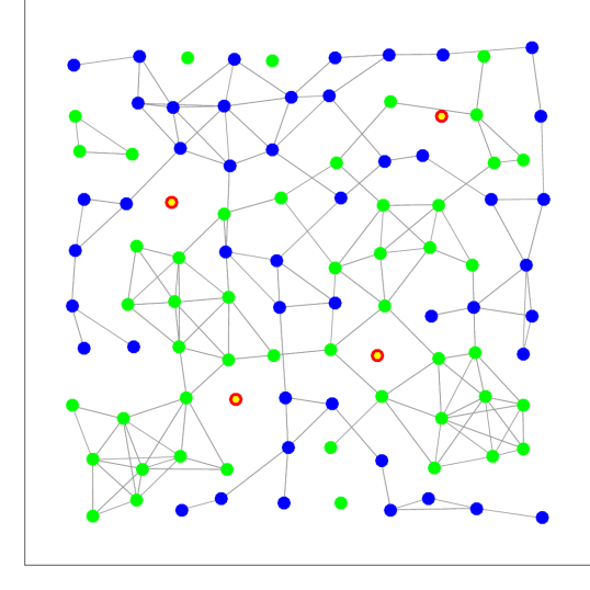
As a result, agents can rely on DLMSAW algorithm for the multi-target localization problem. Figure 2(a) shows the network topology before the application of diffusion algorithms. For better readability, we only illustrate the network topology of agents without showing targets.

For stationary target localization, the location of the two stationary targets are given by

$$w_{k}^{0}=\begin{cases}[0.1,0.1]^{\top},&\text{for }k\text{ depicted in blue}\\ [0.9,0.9]^{\top},&\text{for }k\text{ depicted in green}\end{cases}$$

Non-stationary targets are given by

$$\bm{w}_{k,i}^{0}=\begin{cases}\begin{bmatrix}0.1+0.1\cos(2\pi\omega i)\\ 0.1+0.1\sin(2\pi\omega i)\end{bmatrix},\text{for }k\text{ depicted in blue}\\ \\ \begin{bmatrix}0.9+0.1\cos(2\pi\omega i)\\ 0.9+0.1\sin(2\pi\omega i)\end{bmatrix},\text{for }k\text{ depicted in green}\end{cases}$$

where $\omega=\frac{1}{2000}$.

Regression data is white Gaussian with diagonal covariance matrices $R_{u,k}=\sigma_{u,k}^{2}I_{M}$ with $M=2$, $\sigma_{u,k}^{2}\in[0.8,1.2]$ and noise variance $\sigma_{k}^{2}\in[0.15,0.2]$. The step size of $\mu_{k}=0.01$ and the forgetting factor $\nu_{k}=0.01$ are set uniformly across the network. Note that we adopt a signal-to-noise ratio (SNR) of $5-10$ dB in our setup. However, the same results are generated if we choose low SNR values.

VII-A Strong Attacks

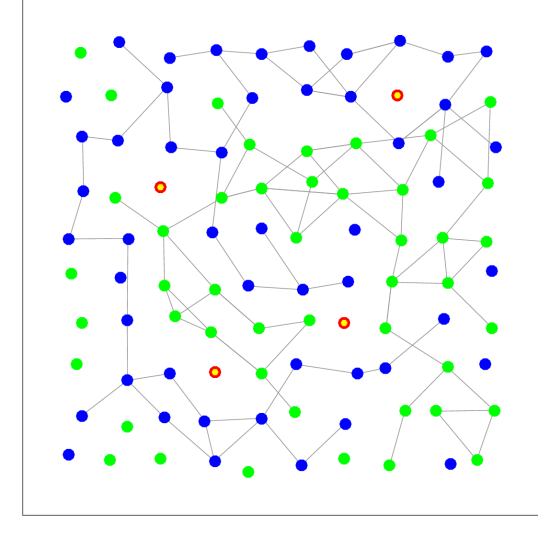
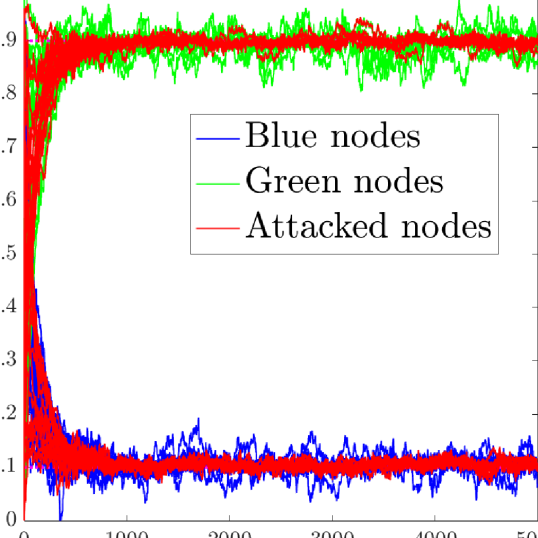
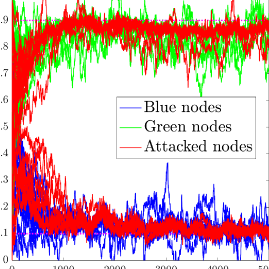
We consider the strong attack model discussed in Sections IV and V. The attacker aims at making the normal agents estimate a specific location selected by the attacker. In this evaluation, we select the attacker’s targeted location to be $w_{k}^{a}=[0.5,0.5]^{\top}$, and the attack parameters are selected uniformly across the compromised agents as $r_{k}^{a}=0.002$. For non-stationary estimation, we select $\theta_{k,i}^{a}=[0.1\cos(2\pi\omega_{a}i),$ $0.1\sin(2\pi\omega_{a}i)]^{\top}$, $\Delta\theta_{k,i}^{a}=[-0.2\pi\omega_{a}\sin(2\pi\omega_{a}i),$ $0.2\pi\omega_{a}\cos(2\pi\omega_{a}i)]^{\top}$, where $\omega_{a}=\frac{1}{2000}$. Figure 2(b) shows the network topology at the end of the simulation using DLMSAW with no attack for both stationary and non-stationary tasks. If the weights between agents $k$ and $l$ are such that $a_{lk}(i)<0.01$ and $a_{kl}(i)<0.01$, then we remove the link between such nodes from the network. We observe that only the links between agents estimating the same target are kept, that is green nodes are connected with green nodes only, and blue nodes are connected with only blue ones, thus, illustrating the robustness of DLMSAW in multi-task networks. Figure 3(a) and Figure 3(b) shows the estimation dynamics by DLMSAW for the targets’ locations $\bm{w}_{k,i}(1)$ and $\bm{w}_{k,i}(2)$ for every agent $k$ and iteration $i$ from 0 to $5000$ under no attack. Here $\bm{w}_{k,i}(1)$ and $\bm{w}_{k,i}(2)$ are the first and second element of the estimate respectively, that is $\bm{w}_{k,i}=[\bm{w}_{k,i}(1),\bm{w}_{k,i}(2)]^{\top}$. It is shown that the two groups of nodes converge to their goal state.

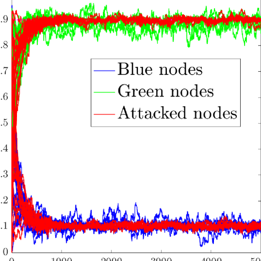
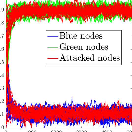
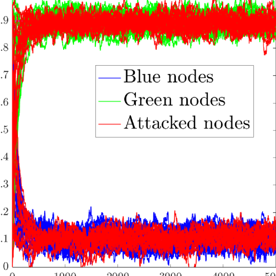
Figure 2(c) shows the initial network topology with compromised nodes. There are four compromised nodes (red nodes with yellow centres) in the network. Figure 2(d) shows the network topology at the end of DLMSAW in the case of a strong attack. All red nodes are the normal agents converging to $w_{k}^{a}$. We observe that neighbors of a compromised node communicate only with the compromised node, and not with any other node in the network. As a result, compromised nodes successfully drive all of their neighbors to desired states $w_{k}^{a}$ as discussed in Section V. Figure 3(c) and Figure 3(d) shows the estimation dynamics by DLMSAW for the targets’ location $\bm{w}_{k,i}(1)$ and $\bm{w}_{k,i}(2)$ for every agent $k$ and iteration from 0 to $5000$ under attack. The attacked nodes in the figure refer to the immediate neighbors of the compromised nodes. It is shown that all the immediate neighbors of compromised nodes are driven to converge to $w_{k}^{a}$ whereas all the other normal nodes converge to their original goal states.

(a) Initial network topology (no compromised nodes)

(b) At the end of DLMSAW with no attack

(c) Initial network topology (with compromised nodes)

(d) At the end of DLMSAW under strong attack

Figure 2: Network topologies in the case of DLMSAW algorithm.

(a) $\bm{w}_{k,i}(1)$ (under no attack)

(b) $\bm{w}_{k,i}(2)$ (under no attack)

(c) $\bm{w}_{k,i}(1)$ (under strong attack)

(d) $\bm{w}_{k,i}(2)$ (under strong attack)

Figure 3: Estimation dynamics for stationary target localization by DLMSAW.

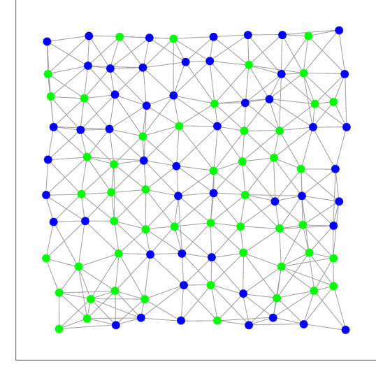
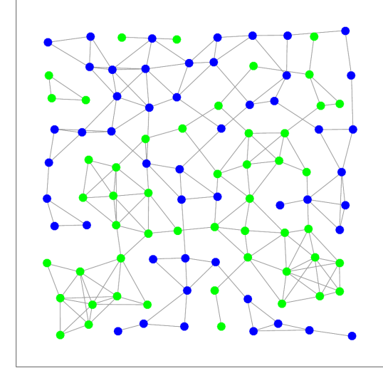
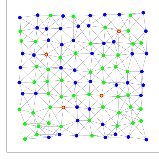
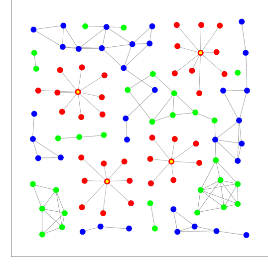
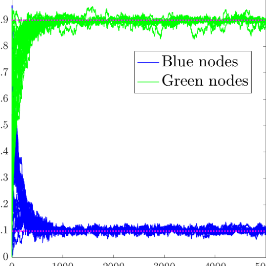
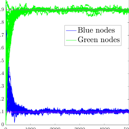
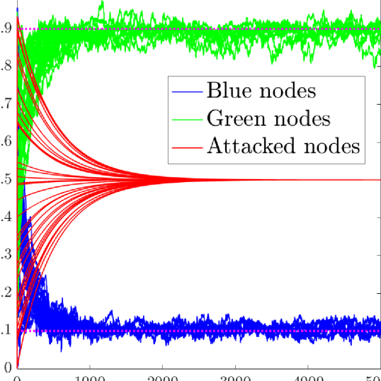
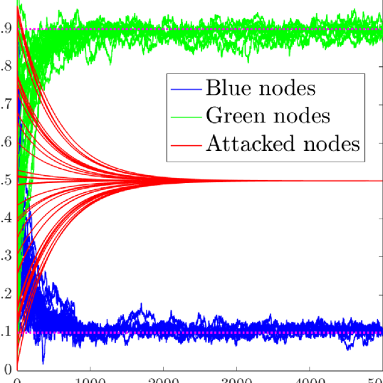
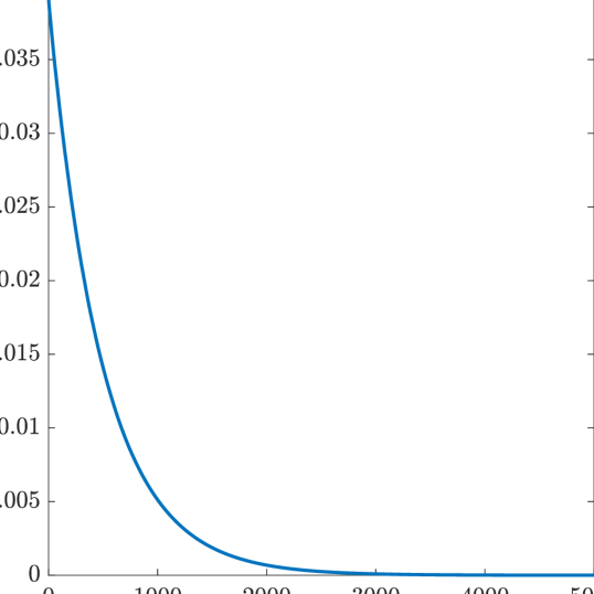
Figure 4(a) shows the convergence of nodes under attack (stationary targets). We note at around 3000 iterations, the difference between the average state of nodes under attack and the attacker’s desired state $w_{k}^{a}$ becomes almost zero. This observation is also consistent with the result in (15), as for $i=3000$ and $r_{k}^{a}=0.002$, the value of $\epsilon$ turns out to be $0.0025$, which is indeed quite small and indicates the convergence of node’s estimate to $w_{k}^{a}$.

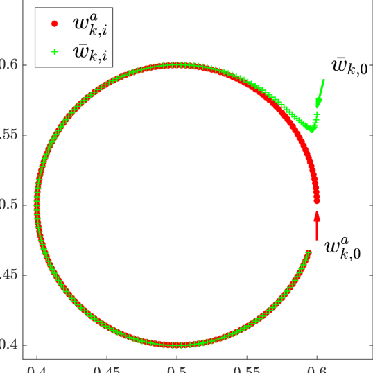
Figure 4(b) shows the average state dynamics of nodes under attack for non-stationary targets. Since states are changing over time, we illustrate the dynamics of average states’ changing with respect to the dynamics of attacker’s selected state, instead of a convergence plot like 4(a). Here, the $X$-coordinate denotes the first element of the estimation vector, i.e., $\bm{w}_{k,i}(1)$, and $Y$-coordinate denotes the second, i.e., $\bm{w}_{k,i}(2)$. At iteration $0$, the average state $\overline{w}_{k,i}$ of the nodes under attack is different than the attacker’s desired state $w_{k,i}^{a}$. As the attack proceeds, $\overline{w}_{k,i}$ gradually converges towards $w_{k,i}^{a}$, which shows the effectiveness of attack for non-stationary state estimation.

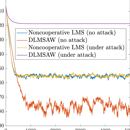
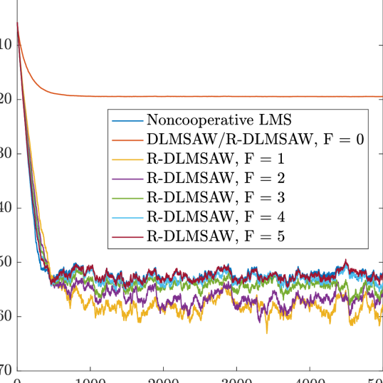
Figure 5 shows the steady-state MSD performance of DLMSAW and non-cooperative LMS. We observe that under no attack, cooperation indeed improves the steady-state MSD performance of DLMSAW. However, in the case of an attack, the steady-state MSD level of DLMSAW is quite high, whereas, the steady-state MSD level of non-cooperative LMS is barely affected by the attack.

(a) Stationary targets

(b) Non-stationary targets

Figure 4: Average state dynamics of compromised nodes’ neighbors
(under strong attack).

(c) Stationary targets

(d) Non-stationary targets

Figure 5: Steady-state MSD levels in non-cooperative LMS
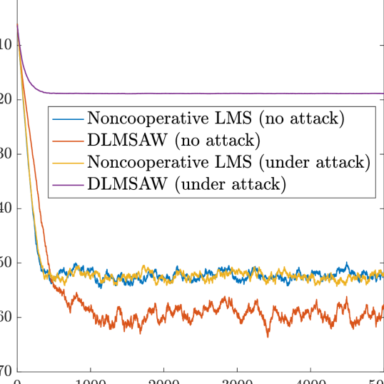
and DLMSAW (under strong attack).

VII-B Resilient Diffusion for Strong Attacks

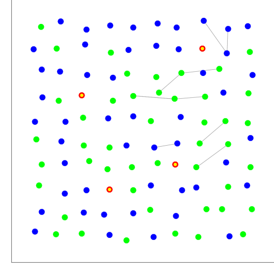
To evaluate R-DLMSAW, we compute the cost $J_{k}(\bm{\psi}_{l,i})$ using the streaming data from the latest 100 iterations. We adopt uniform $F$ for every normal agent but it can be distinct for each agent. R-DLMSAW behaves identically to DLMSAW at one extreme, that is when $F=0$, and on the other extreme it behaves like a non-cooperative LMS algorithm, that is for large $F$. We consider the same initial network as in Figure 2(a) and consider an attack consisting of four compromised nodes as previously. Note that there is at most one compromised node in the neighborhood of a normal agent. Figure 6 shows network topologies after executing R-DLMSAW for various values of $F$. Since there is at most one compromised node in the neighborhood of a normal agent, the selection of $F=1$ should be sufficient to guarantee that none of the normal nodes converge to attacker’s desired states, which is indeed the case as indicated by the removal of all links between normal and compromised nodes in Figure 6(a). As we increase $F$, resilience against attack is certainly achieved, but at the same time the network becomes sparser as illustrated in Figures 6(b) and 6(c). In the case of non-stationary state estimation, the resulting network topologies are similar, and hence, are not presented.

Figure 7 shows the estimation dynamics by R-DLMSAW for the targets’ location $\bm{w}_{k,i}(1)$ and $\bm{w}_{k,i}(2)$ for every agent $k$ and iteration $i$ from 0 to $5000$ under attack. The attacked nodes in the figure refer to the immediate neighbors of the compromised nodes. Since there is at most one compromised node in a normal node’s neighborhood, setting $F\geq 1$ will make R-DLMSAW algorithm resilient to attacks, which is demonstrated by the results from the figure. We also observe that by setting a smaller $F$ value, which is sufficient to to make the algorithm resilient, we achieve better estimation performance ($F=1$ has less noise than that of $F=5$).

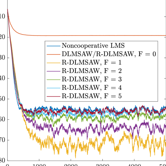
Figure 8 shows the steady-state MSD level of the network for the three algorithms, that is, non-cooperative LMS, DLMSAW, and R-DLMSAW. The simulation results validate claims in Section VI. We observe that in the presence of compromised nodes, DLMSAW performs the worst and has the highest steady-state MSD. Since there is at most one compromised node in the neighborhood of any normal node, the most appropriate value of $F$ for R-DLMSAW is 1. We note that the steady-state MSD is indeed minimum for $F=1$. As we increase $F$, the steady-state MSD also increases. In fact, for $F=5$, the performance of R-DLMSAW and non-cooperative LMS is almost the same as we expect.

(a) $F=1$

(b) $F=3$

(c) $F=5$

Figure 6: Network topologies at the end of R-DLMSAW under strong attack (stationary targets) for various values of $F$.

(a) $\bm{w}_{k,i}(1)$ ($F=1$)

(b) $\bm{w}_{k,i}(2)$ ($F=1$)

(c) $\bm{w}_{k,i}(1)$ ($F=5$)

(d) $\bm{w}_{k,i}(2)$ ($F=5$)

Figure 7: Estimation dynamics for stationary target localization by R-DLMSAW under strong attack.

(a) Stationary targets

(b) Non-stationary targets

Figure 8: A comparison of MSD performance of non-cooperative LMS, DLMSAW, and R-DLMSAW under strong attack.

VIII Weak Attacks

Though it is common to assume a strong attacker with complete knowledge when examining the resilience of a distributed system, it is interesting to examine what an attacker can do in practise if all the information is not available. In this section, we analyze how the attack can still be deployed on a normal agent $k$ without the assumption of a strong knowledge by the attacker (streaming data and parameters used by $k$). We assume that an attacker has access only to the intermediate estimates shared by agents with others in their neighborhood. For instance, if $l\in\mathcal{N}_{k}$ then agent $k$ receives $\bm{\psi}_{l,i}$ from $l$ and attacker also has an access to it. We show that the other knowledge needed by the attacker can actually be approximated in an alternative way, and the success of the attack relies on how accurate this information can be approximated. We refer to such an attack in which attacker can only gather intermediate estimates and not the other data (including streaming data and agent parameters) as the weak attack.

The strong attack in (10) relies essentially on the knowledge of $\bm{w}_{k,i-1}$, that is the estimated state of agent $k$ in the last iteration. If the attacker has complete knowledge, it can compute $\bm{w}_{k,i-1}$ exactly as Lemma 1 indicates. However, without such knowledge, $\bm{w}_{k,i-1}$ can only be approximately computed. We note that approximating $\bm{w}_{k,i-1}$ is equivalent to approximating the weight matrix $A_{k}(i)=[a_{lk}(i)],\forall l\in\mathcal{N}_{k}$. This is true because $\bm{w}_{k,i}=\sum_{l\in N_{k}}a_{lk}(i)\bm{\psi}_{l,i}$, and $\bm{\psi}_{l,i}$ is received by the attacker $a$ from $l$.

Next, we discuss how to compute the approximated weight matrix $\hat{A}_{k}(i-1)$ using only the information $\bm{\psi}_{l,i},\forall l\in\mathcal{N}_{k}$. Note that the adaptation step (2) of diffusion can be written as,

$$\bm{\psi}_{k,i}=\bm{w}_{k,i-1}+\nabla_{k,i}=A_{k}(i-1)\Psi_{k,i-1}+\nabla_{k,i}.$$

where $\nabla_{k,i}=\mu_{k}\bm{u}_{k,i}^{*}(\bm{d}_{k}(i)-\bm{u}_{k,i}\bm{w}_{k,i-1})$, $\Psi_{k,i-1}$ is an $|\mathcal{N}_{k}|\times M$ matrix $\Psi_{k,i-1}=[\bm{\psi}_{l,i-1}],\forall l\in\mathcal{N}_{k}$. Thus,

$$\nabla_{k,i}=\bm{\psi}_{k,i}-A_{k}(i-1)\Psi_{k,i-1},$$

and therefore,

$$\lim_{i\rightarrow\infty}\mathbb{E}\{\|\nabla_{k,i}\|^{2}\}=\lim_{i\rightarrow\infty}\mathbb{E}\{\|\bm{\psi}_{k,i}-A_{k}(i-1)\Psi_{k,i-1}\|^{2}\}.$$

Since $\lim_{i\rightarrow\infty}\mathbb{E}\{\|\nabla_{k,i}\|^{2}\}=0$, the value of $A_{k}(i)$ can be approximated by assigning a cost function

$$\ell(A_{k}(i))\triangleq\mathbb{E}\{\|\bm{\psi}_{k,i+1}-A_{k}(i)\Psi_{k,i}\|^{2}\},$$

where $A_{k}(i)$ is the global minimizer of $\ell(A_{k}(i))$ as $i\rightarrow\infty$. Next, we compute the successive estimators of the weight matrix based on stochastic gradient descent method as follows:

$$\hat{A}_{k}(i) =\hat{A}_{k}(i-1)-\mu^{\prime}_{A}\nabla_{A}\ell(\hat{A}_{k}(i-1))$$ (20)

$$=\hat{A}_{k}(i-1)+\mu_{A}\Psi_{k,i-1}(\bm{\psi}_{k,i}-\hat{A}_{k}(i-1)\Psi_{k,i-1}),$$

where $\mu_{A}=\frac{1}{2}\mu^{\prime}_{A}$.

Also recall weight matrix $A_{k}(i)$ has to satisfy the condition (4). Thus, to make the adaptive approximation of weight matrix hold condition (4), we introduce two more steps following (20), that is the clip step and the normalization step. In the clip step, the negative weights are clipped and are set to zero; and the in the normalization step, weights are divided by their sum. The operation for approximating weight matrix of a normal agent $k$ is summarized in Algorithm 2.

Input: $l\in N_{k}$, randomized $a_{lk}(0)$ satisfying (4), $\mu_{A}$, $\bm{\psi}_{k,i}$, $\Psi_{k,i-1}$

1 for $i>0$ do

2       $A_{k}(i)=A_{k}(i-1)+\mu_{A}\Psi_{k,i-1}(\bm{\psi}_{k,i}-A_{k}(i-1)\Psi_{k,i-1})$

3       for $l\in\mathcal{N}_{k}$ do

4             $a_{lk}(i)=\max(a_{lk}(i),0)$

5      $A_{k}(i)=\frac{A_{k}(i)}{\sum a_{lk}(i)}$

6       return $A_{k}(i)$

Algorithm 2 Approximate weight matrix for agent $k$

We then approximate normal agent $k$’s estimated state by

$$\hat{\bm{w}}_{k,i}=\hat{A}_{k}(i)\Psi_{k,i},$$

and use $\hat{\bm{w}}_{k,i}$ instead of $\bm{w}_{k,i}$. The attack model in (10) then becomes

$$\bm{\psi}_{a,i}=\hat{\bm{w}}_{k,i-1}+r_{k}^{a}(x_{i}-\hat{\bm{w}}_{k,i-1}).$$ (21)

Note that the sufficient condition listed in Proposition 1 guarantees the convergence of the attack objective. However, without an exact knowledge of $\bm{w}_{k,i-1}$ it is not guaranteed the sufficient condition can be satisfied. In other words, the success of the attack relies highly on how accurate the state $\hat{\bm{w}}_{k,i}$ can be approximated. In the following, we provide evaluation results for such an attack.

VIII-A Evaluation

We adopt the same evaluation set-up as we used in section vii@. Initial network topology is the same as in 2(a). Parameters we select are: $\sigma_{u,k}^{2}\in[0.75,0.85]$, $\sigma_{k}^{2}\in[0.75,0.85]$ for each agent $k$ and $\mu_{A}=0.002$, while all the other settings are the same as in section vii@.

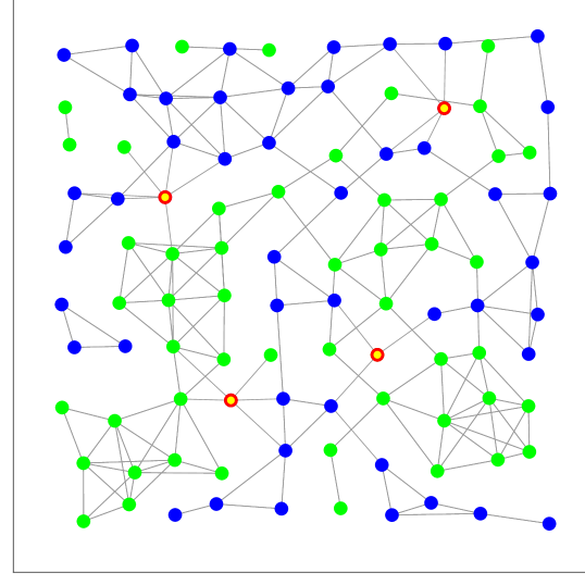
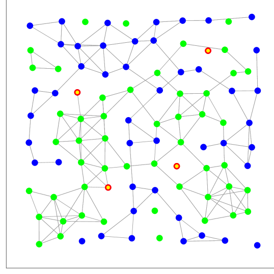
At the end of DLMSAW under weak attack, we reach the network topology as shown in Figure 9(a). From the plots, we find some of the agents maintain connection with the compromised nodes, while others do not, which is not the case with a strong attack, where all the neighboring agents of a compromised node end up cooperating only with the compromised node. The main reason for this is that the weak attack may not have an accurate approximation of normal agents’ state. Without an accurate approximation, compromised nodes may not be able to collect large weights from their neighbors and may not keep influencing the states of their neighbors.

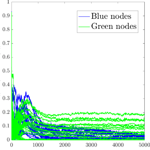
Figure 11 illustrates the estimation precision ($\|\hat{\bm{w}}_{k,i}-\bm{w}_{k,i}\|$) by the attacker. It shows that the attacker has different levels of accuracy to estimate the states of its neighboring agents. For some agents, the attacker has accurate approximation along the simulation iterations. As a result, the attacker is more likely to make its attack successful on those agents. However, for other agents, the attacker does not have very good approximation accuracy and therefore, it is hard for the attacker to successfully attack such agents. Figure 13 shows the state estimation dynamics of normal agents (wherein attacked nodes refer to the neighboring nodes of the compromised nodes). We find the attacker can only drive a few of its neighbors to its desired state, whereas most of the normal neighbors converge to their true goal state, which is consistent with the results of Figure 11. The steady-state MSD performance for the weak attack is shown in the yellow line in Figure 11. We find that such an attack still worsens the network steady-state MSD as compared to the non-cooperative LMS (the blue line) and DLMSAW without attack (the red line).

Next, we evaluate the proposed resilient diffusion algorithm R-DLMSAW against the weak attack. The network topology at the end of simulation is shown in Figure 9(b). Most normal agents have cut the link with the compromised nodes. Yet some links are maintained because these compromised nodes behave in a benign way as to send message with a smaller cost than a normal neighbor of the targeted node. In other words, these compromised nodes exchange a state message similar to normal nodes in order to maintain communication with them. Therefore, such links need not to be cut down to achieve the network resilience. Figure 13 shows the estimation dynamics of normal nodes by R-DLMSAW. We find none of the attacked nodes are driven to the attacker’s selected state. All the nodes successfully converge to their true goal states. The purple line in Figure 11 shows the steady-state MSD performance of R-DLMSAW with $F=1$. We observe that this line lies between the noncooperative LMS and DLMSAW (without attack), and has a much smaller steady-state MSD than DLMSAW under such attack. This illustrates the effectiveness of the proposed resilient diffusion algorithm by showing that the algorithm is resilient to not only strong but also to weak attacks, as well as other data falsification attacks.

(a) DLMSAW

(b) R-DLMSAW

Figure 9: Network topologies at the end of simulation
under weak attack.

Figure 10: Sate estimation
precision.

Figure 11: Steady-state MSD
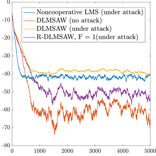
comparison under weak attack.

(a) $\bm{w}_{k,i}(1)$

(b) $\bm{w}_{k,i}(2)$

Figure 12: Estimation dynamics for stationary target localization
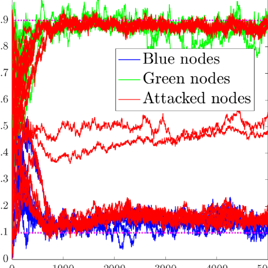
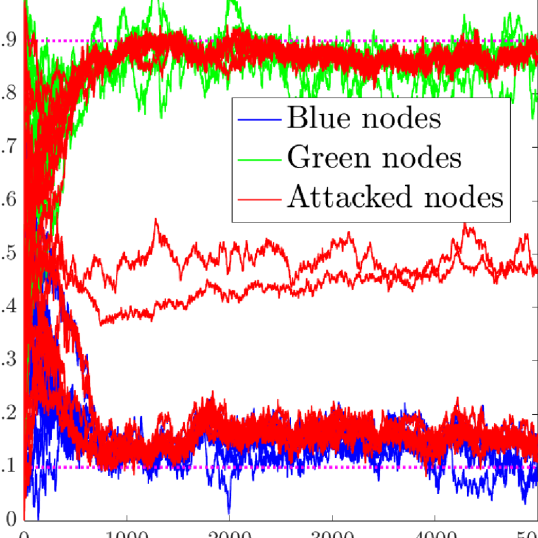
by DLMSAW under weak attack.

(c) $\bm{w}_{k,i}(1)(F=1)$

(d) $\bm{w}_{k,i}(2)(F=1)$

Figure 13: Estimation dynamics for stationary target localization
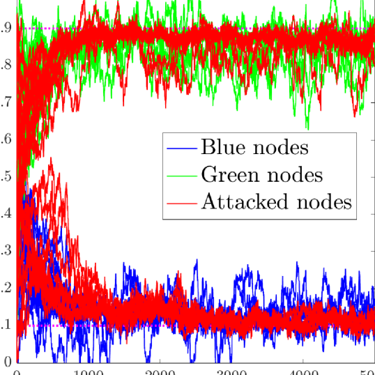
by R-DLMSAW under weak attack.

IX Related Work

Many distributed algorithms are vulnerable to cyber attacks. The existence of an adversarial agent may prevent the algorithm from performing the desired task. Distributed consensus and diffusion based strategies are often employed to resolve distributed estimation and optimization problems, for instance see [19, 20, 21, 22, 23, 2]. Resilience of consensus-based distributed algorithms in the presence of malicious nodes has received considerable attention in recent years. In particular, the approaches presented in [24, 25, 11, 26] consider the consensus problem for scalar parameters in the presence of attackers, and resilience is achieved by leveraging high connectivity. Resilient consensus in the case of special network structures, such as triangular networks for distributed robotic applications [27], has also been studied. To achieve resilience in sparse networks, [28] presents the idea of employing few trusted nodes, which are hardened nodes that cannot be attacked. Resilience for concensus+innovation problems have also been studied by [29, 30, 31] in a fully-distributed way via agents’ local observations and high network connectivity. Resilience can also be achieved via fault detection and isolation (FDI). For instance, [32] studied the FDI problem for linear consensus networks via high connectivity networks and global knowledge of the network structure by each agent. [33] considered a similar FDI problem for second-order systems. Authors in [34] presented distributed detection method for consensus+innovation algorithms via local observations of agents only. For attacks, typical approaches usually consider Byzantine adversaries with fixed target different than the true value [11] or with updates without time-dependent intention [34, 30] and assume that the goal of the attacker is to disrupt the convergence (stability) of the distributed algorithm. In contrast, this work focuses on attacks that do not disrupt convergence but drive normal agents to converge to states selected by the attacker. Moreover, in our attack model, the attacker continuously changes its values over time as compared to the fixed value attacks considered previously.

Resilience of diffusion-based distributed algorithms has been studied in [2, 5, 8]. Similar to the resilient consensus problems, fixed-value attacks are usually considered, and the main approach has been to use adaptive combination rules to counteract malicious values. This is an effective measure and has been applied to multi-task networks and distributed clustering problems [5]. Several variants focusing on adaptive weights applied to multi-task networks can be found in [35, 36, 18, 37]. Note that the essence of adaptive weights is similar to distributed detection. In contrast, it turns the detection method from a binary classification problem to a regression problem. Detection approach has also been applied in [35] for clustering over diffusion networks. Although adaptive weights provide some degree of resilience to byzantine adversaries with fixed values, we have shown in this work that adaptive weights may introduce vulnerabilities that allow time-dependent deception attacks.

Finally, there has been considerable work on applications of diffusion algorithms that include spectrum sensing in cognitive networks [3], target localization [4], distributed clustering [5], biologically inspired designs [6]. Although our approach can be used for resilience of various applications, we have focused on multi-target localization [18].

X Conclusions

In this paper, we studied distributed diffusion for multi-task networks and investigated vulnerabilities introduced by adaptive weights. Cooperative diffusion is a powerful strategy to perform optimization and estimation tasks, however, its performance and accuracy can deteriorate significantly in the presence of adversarial nodes. In fact, cooperative diffusion performs significantly better (in terms of steady-state MSD) as compared to non-cooperative diffusion if there are no adversarial nodes. However, with adversaries, cooperative diffusion could be even worse than the non-cooperative diffusion. To illustrate this, we proposed attack models that can drive normal agents—implementing distributed diffusion (DLMSAW)—to any state selected by the attacker, for both stationary and non-stationary estimation. We then proposed a resilient distributed diffusion algorithm (R-DLMSAW) to counteract adversaries’ effect. The proposed algorithm always performs at least as good as the non-cooperative diffusion, but if an input parameter $F$ in the algorithm is selected appropriately, it performs significantly better than the non-cooperative diffusion in the presence of adversaries. We also analyzed how the performance of R-DLMSAW changes with the selection of parameter $F$ by the nodes. We evaluated our approach by applying it to stationary and non-stationary multi-target localization. In future, we are interested in generalizing our model to other types of distributed diffusion algorithms and with the missing data. It is also worth investigating the relationship between the underlying network connectivity and the steady-state performance of such algorithms.

Appendix

Proof of Lemma 1

The message received by $a$ from $k\in\mathcal{N}_{a}$ is $\bm{\psi}_{k,i}$. Agent $a$ can compute $\bm{w}_{k,i-1}$ from $\bm{\psi}_{k,i}$ using

$$\bm{w}_{k,i-1}=\bm{\psi}_{k,i}-\mu_{k}\bm{u}_{k,i}^{*}(\bm{d}_{k}(i)-\bm{u}_{k,i}\bm{w}_{k,i-1}),$$

from which it can compute $\bm{w}_{k,i-1}$ as:

$$\bm{w}_{k,i-1}=\frac{\bm{\psi}_{k,i}-\mu_{k}\bm{u}_{k,i}^{*}\bm{d}_{k}(i)}{1-\mu_{k}\bm{u}_{k,i}^{*}\bm{u}_{k,i}}.$$

Given the knowledge of $\mu_{k}$, $\bm{d}_{k}(i)$, and $\bm{u}_{k,i}$, the value $\bm{w}_{k,i-1}$ can be computed exactly.

Proof of Lemma 2

We use $\delta_{a,k,i}$ to denote $\|\bm{\psi}_{a,i}-\bm{w}_{k,i-1}\|$, and $\delta_{l,k,i}$ to denote $\|\bm{\psi}_{l,i}-\bm{w}_{k,i-1}\|$, for $l\in\mathcal{N}_{k},l\neq a$. Since

$$\gamma_{lk}^{2}(i)=(1-\nu_{k})\gamma_{lk}^{2}(i-1)+\nu_{k}\|\bm{\psi}_{l,i}-\bm{w}_{k,i-1}\|^{2},l\in\mathcal{N}_{k},$$

Suppose the attack starts at $i_{a}$, then at iteration $(i_{a}+n)$,

$$\begin{split}&\gamma^{2}_{ak}(i_{a}+n)\\ =&(1-\nu_{k})\gamma^{2}_{ak}(i_{a}+n-1)+\nu_{k}\delta_{a,k,i_{a}+n}^{2}\\ =&(1-\nu_{k})((1-\nu_{k})\gamma^{2}_{ak}(i_{a}+n-2)+\nu_{k}\delta_{a,k,i_{a}+n-1}^{2})\\ &+\nu_{k}\delta_{a,k,i_{a}+n}^{2}\\ =&(1-\nu_{k})^{n+1}\gamma^{2}_{ak}(i_{a}-1)\\ &+\nu_{k}[(1-\nu_{k})^{n}\delta_{a,k,i_{a}}^{2}+(1-\nu_{k})^{n-1}\delta_{a,k,i_{a}+1}^{2}\\ &+\ldots+(1-\nu_{k})\delta_{a,k,i_{a}+n-1}^{2}+\delta_{a,k,i_{a}+n}^{2}],\end{split}$$

$$\begin{split}\gamma^{2}_{lk}(i_{a}+n)=&(1-\nu_{k})^{n+1}\gamma^{2}_{lk}(i_{a}-1)\\ &+\nu_{k}[(1-\nu_{k})^{n}\delta_{l,k,i_{a}}^{2}+(1-\nu_{k})^{n-1}\delta_{l,k,i_{a}+1}^{2}\\ &+\ldots+(1-\nu_{k})\delta_{l,k,i_{a}+n-1}^{2}+\delta_{l,k,i_{a}+n}^{2}].\end{split}$$

For large enough $n$, $(1-\nu_{k})^{n+1}\rightarrow 0$. Since we assume $\|\bm{\psi}_{a,i}-\bm{w}_{k,i-1}\|\ll\|\bm{\psi}_{l,i}-\bm{w}_{k,i-1}\|$, i.e., $\delta_{a,k,i}\ll\delta_{l,k,i}$, for $i\geq i_{a}+n$, $\gamma^{2}_{ak}(i)\ll\gamma^{2}_{lk}(i)$ holds. Thus,

$$\frac{a_{lk}(i)}{a_{ak}(i)}\propto\frac{\gamma^{-2}_{lk}(i)}{\gamma^{-2}_{ak}(i)}\rightarrow 0.$$ (22)

Given the property of weights, (13) is true.

Proof of Lemma 3

We use $\mathcal{A}$ to denote the set of compromised nodes targeting at the same normal node $k$. The proposed attack strategy results in the following condition holding as proved in Lemma 2:

$$\begin{split}&\frac{a_{lk}(i)}{a_{ak}(i)}\rightarrow 0,\qquad l\in\mathcal{N}_{k}\backslash\mathcal{A},a\in\mathcal{A},\\ &(i\geq i_{a}+n,\text{ subject to }(1-\nu_{k})^{n+1}=0).\end{split}$$

Given that $\sum_{l\in\mathcal{N}_{k}}a_{lk}=1$, we have

$$a_{lk}(i)=0,a_{ak}(i)=\frac{1}{|\mathcal{A}|},\qquad l\in\mathcal{N}_{k}\backslash\mathcal{A},a\in\mathcal{A},$$

where $|\mathcal{A}|$ denotes the number of nodes in $\mathcal{A}$. Since every compromised node $a\in\mathcal{A}$ sends the same message and is assigned the same weight that sums up to 1, it is equivalent to only one compromised node attacking the target node and being assigned a weight of 1. Therefore, there is no need for multiple compromised nodes attacking a single normal node.

Proof of Proposition 1

The constraint of $r_{k}^{a}$ is consistent with the condition of Lemma 2. Thus, from some point $i$, the state of node $k$ will be attacked as to be:

$$\begin{split}\bm{w}_{k,i}&=\bm{w}_{k,i-1}-r_{k}^{a}(\bm{w}_{k,i-1}-x_{i})\\ &=r_{k}^{a}x_{i}+(1-r_{k}^{a})\bm{w}_{k,i-1},\\ &(i\geq i_{a}+n,\text{ subject to }(1-\nu_{k})^{n+1}=0).\end{split}$$ (23)

Let $X_{i}$ be $\bm{w}_{k,i}$, $X_{i-1}$ be $\bm{w}_{k,i-1}$, $A_{i}$ be $r_{k}^{a}x_{i}$, and $B$ be $(1-r_{k}^{a})$. Equation (23) turns to:

$$X_{i}=A_{i}+BX_{i-1}.$$ (24)

Assume $\lim_{i\rightarrow\infty}X_{i-1}=X_{i-1}^{0}$ and $\lim_{i\rightarrow\infty}X_{i}=X_{i}^{0}$, then for $i\rightarrow\infty$ we get:

$$X_{i}^{0}=A_{i}+BX_{i-1}^{0}.$$ (25)

Subtract (25) from (24), we get $X_{i}-X_{i}^{0}=B(X_{i-1}-X_{i-1}^{0}).$ Let $\varepsilon_{i}=X_{i}-X_{i}^{0}$, for $i=0,1,2,\ldots$, then $\varepsilon_{i}=B\varepsilon_{i-1}=B^{2}\varepsilon_{i-2}=\ldots=B^{i}\varepsilon_{0}$. The necessary and sufficient requirement for convergence is $\lim_{i\to\infty}\varepsilon_{i}=0$ or, $\lim_{i\to\infty}B^{i}\varepsilon_{0}=0$, that is,

$$\lim_{i\to\infty}B^{i}=0.$$ (26)

Therefore, we get a necessary and sufficient requirement for convergence as $|B|<1$. Since $B=1-r_{k}^{a}$, and $r_{k}^{a}\in(0,1)$, we get $B\in(0,1)$. Therefore, $\lim_{i\rightarrow\infty}(X_{i}-X_{i}^{0})=0$. The assumption $\lim_{i\rightarrow\infty}X_{i}=X_{i}^{0}$ holds, and therefore, $X_{i}$ is convergent to $X_{i}^{0}$.

To get the value of $X_{i}^{0}$, we need to analyze the following two scenarios: stationary state estimation and non-stationary state estimation, separately.

-1 Stationary state estimation

In stationary scenarios, the convergence state is independent of time, that is, $X_{i}^{0}=X_{i-1}^{0}=X^{0}$. Therefore, equation (25) turns to:

$$X^{0}=A_{i}+BX^{0}.$$

Thus, $(1-B)X^{0}=A_{i}$, $X^{0}=\frac{A_{i}}{1-B}$. The convergent point is:

$$\bm{w}_{k,i}=\frac{r_{k}^{a}x_{i+1}}{1-(1-r_{k}^{a})}=\frac{r_{k}^{a}w_{k}^{a}}{1-(1-r_{k}^{a})}=w_{k}^{a}=\bm{w}_{k,i}^{a},\quad i\rightarrow\infty$$

which realizes the attacker’s objective (7).

-2 Non-stationary state estimation

In non-stationary scenarios, we first assume $x_{i}=w_{k}^{a}+\theta_{k,i-1}^{a}$ and later we will show how $\theta_{k,i-1}^{a}$ turns to $\theta_{k,i-1}^{a}+\frac{\Delta\theta_{k,i-1}^{a}}{r_{k}^{a}}$.

Assume the convergence point $X_{i}^{0}$ is a combination of a time-independent value and a time-dependent value, such that $X_{i}^{0}=X^{0}+\rho_{i}$. After taking original values into (25), we get

$$X^{0}+\rho_{i}=r_{k}^{a}(w_{k}^{a}+\theta_{k,i-1}^{a})+(1-r_{k}^{a})(X_{0}+\rho_{i-1}).$$ (27)

Next, we divide (27) into the time-independent and time-dependent components to get

$$X^{0}=w_{k}^{a},\quad\rho_{i}-\rho_{i-1}=r_{k}^{a}(\theta_{k,i-1}^{a}-\rho_{i-1}).$$

Let $\Delta\rho_{i-1}=\rho_{i}-\rho_{i-1}$, we get:

$$\rho_{i-1}=\theta_{k,i-1}^{a}-\frac{\Delta\rho_{i-1}}{r_{k}^{a}}\quad\text{ and }\quad\rho_{i}=\theta_{k,i}^{a}-\frac{\Delta\rho_{i}}{r_{k}^{a}}.$$ (28)

Thus, $\Delta\rho_{i-1}=\rho_{i}-\rho_{i-1}=\theta_{k,i}^{a}-\theta_{k,i-1}^{a}-\frac{1}{r_{k}^{a}}(\Delta\rho_{i}-\Delta\rho_{i-1})$. Let $\Delta\theta_{k,i-1}^{a}=\theta_{k,i}^{a}-\theta_{k,i-1}^{a}$ and $\Delta^{2}\rho_{i-1}=\Delta\rho_{i}-\Delta\rho_{i-1}$, then $\Delta\rho_{i-1}=\Delta\theta_{k,i-1}^{a}-\frac{\Delta^{2}\rho_{i-1}}{r_{k}^{a}}\quad\text{ or }\quad\Delta\rho_{i}=\Delta\theta_{k,i}^{a}-\frac{\Delta^{2}\rho_{i}}{r_{k}^{a}}$. If we assume $\frac{\Delta^{2}\rho_{i}}{r_{k}^{a}}\ll\Delta\theta_{k,i}^{a}$, then we have $\Delta\rho_{i}=\Delta\theta_{k,i}^{a}$. Therefore, (28) can be written as $\rho_{i}=\theta_{k,i}^{a}-\frac{\Delta\theta_{k,i}^{a}}{r_{k}^{a}}.$ Thus, the dynamic convergence point for $k$ is

$$\bm{w}_{k,i}=w_{k}^{a}+\theta_{k,i}^{a}-\frac{\Delta\theta_{k,i}^{a}}{r_{k}^{a}},\qquad i\rightarrow\infty.$$

This means when sending ${\bm{\psi}}_{a,i}=\bm{w}_{k,i-1}+r_{k}^{a}(w_{k}^{a}+\theta_{k,i-1}^{a}-\bm{w}_{k,i-1})$ as the communication message, the compromised node $a$ can make $k$ converge to $w_{k}^{a}+\theta_{k,i}^{a}-\frac{\Delta\theta_{k,i}^{a}}{r_{k}^{a}}$. To make agent $k$ converge to a desired state $w_{k}^{a}+\Omega_{k,i}^{a}$, we assume the message sent is

$${\bm{\psi}}_{a,i}=\bm{w}_{k,i-1}+r_{k}^{a}(w_{k}^{a}+m_{i-1}-\bm{w}_{k,i-1}).$$

The corresponding convergence point will be $w_{k}^{a}+m_{i}-\frac{\Delta m_{i}}{r_{k}^{a}}$. We want the following equation to hold,

$$w_{k}^{a}+m_{i}-\frac{\Delta m_{i}}{r_{k}^{a}}=w_{k}^{a}+\Omega_{k,i}^{a}.$$ (29)

Assuming $\Delta^{2}m_{i}\rightarrow 0$, the solution of (29) is: $m_{i}=\Omega_{k,i}^{a}+\frac{\Delta\Omega_{k,i}^{a}}{r_{k}^{a}}$, meaning to make $k$ converge to a desired state $w_{k}^{a}+\Omega_{k,i}^{a}$, the compromised node $a$ should send communication message:

$${\bm{\psi}}_{a,i}=\bm{w}_{k,i-1}+r_{k}^{a}(w_{k}^{a}+\Omega_{k,i-1}^{a}+\frac{\Delta\Omega_{k,i-1}^{a}}{r_{k}^{a}}-\bm{w}_{k,i-1}).$$

Thus, to make $k$ converge to $w_{k}^{a}+\theta_{k,i}^{a}$, the compromised node $a$ should send communication message:

$${\bm{\psi}}_{a,i}=\bm{w}_{k,i-1}+r_{k}^{a}(w_{k}^{a}+\theta_{k,i-1}^{a}+\frac{\Delta\theta_{k,i-1}^{a}}{r_{k}^{a}}-\bm{w}_{k,i-1}).$$

The convergence point is:

$$\bm{w}_{k,i}=w_{k}^{a}+\theta_{k,i}^{a}=\bm{w}_{k,i}^{a},\qquad i\rightarrow\infty,$$

which realizes the attacker’s objective (7).

We can verify the convergence point by putting $x_{i}=w_{k}^{a}+\theta_{k,i-1}^{a}+\frac{\Delta\theta_{k,i-1}^{a}}{r_{k}^{a}},\bm{w}_{k,i}=w_{k}^{a}+\theta_{k,i}^{a},\bm{w}_{k,i-1}=w_{k}^{a}+\theta_{k,i-1}^{a}$ back into equation (23), we get:

$$\begin{split}w_{k}^{a}+\theta_{k,i}^{a}&=r_{k}^{a}(w_{k}^{a}+\theta_{k,i-1}^{a}+\frac{\Delta\theta_{k,i-1}^{a}}{r_{k}^{a}})+(1-r_{k}^{a})(w_{k}^{a}+\theta_{k,i-1}^{a})\\ \theta_{k,i}^{a}&=r_{k}^{a}(\theta_{k,i-1}^{a}+\frac{\Delta\theta_{k,i-1}^{a}}{r_{k}^{a}})+(1-r_{k}^{a})\theta_{k,i-1}^{a}\\ \theta_{k,i}^{a}&=\theta_{k,i-1}^{a}+\Delta\theta_{k,i-1}^{a}.\end{split}$$

The resulting equation holds, illustrating the validity of the convergence state.

References

- [1] J. Li and X. Koutsoukos, “Resilient distributed diffusion for multi-task estimation,” in 14th International Conference on Distributed Computing in Sensor Systems (DCOSS). IEEE, 2018, pp. 93–102.
- [2] A. H. Sayed, S.-Y. Tu, J. Chen, X. Zhao, and Z. J. Towfic, “Diffusion strategies for adaptation and learning over networks: An examination of distributed strategies and network behavior.” IEEE Signal Processing Magazine, vol. 30, no. 3, pp. 155–171, 2013.
- [3] J. Plata-Chaves, N. Bogdanović, and K. Berberidis, “Distributed diffusion-based LMS for node-specific adaptive parameter estimation,” IEEE Transactions on Signal Processing, vol. 63, pp. 3448–3460, 2015.
- [4] A. Lotfzad Pak, A. Khalili, M. K. Islam, and A. Rastegarnia, “A distributed target localization algorithm for mobile adaptive networks,” ECTI Transactions on Electrical Engineering, Electronics, and Communications, vol. 14, pp. 47–56, 08 2016.
- [5] X. Zhao and A. H. Sayed, “Clustering via diffusion adaptation over networks,” in 3rd International Workshop on Cognitive Information Processing, May 2012, pp. 1–6.
- [6] S.-Y. Tu and A. H.Sayed, “Mobile adaptive networks,” IEEE Journal of Selected Topics in Signal Processing, vol. 5, no. 4, pp. 649–664, 2011.
- [7] J. Chen and A. H. Sayed, “Diffusion adaptation strategies for distributed optimization and learning over networks,” IEEE Transactions on Signal Processing, vol. 60, no. 8, pp. 4289–4305, Aug 2012.
- [8] S. Chouvardas, K. Slavakis, and S. Theodoridis, “Adaptive robust distributed learning in diffusion sensor networks,” IEEE Transactions on Signal Processing, vol. 59, no. 10, pp. 4692–4707, Oct 2011.
- [9] R. Nassif, C. Richard, A. Ferrari, and A. H. Sayed, “Proximal multitask learning over networks with sparsity-inducing coregularization,” IEEE Transactions on Signal Processing, vol. 64, no. 23, pp. 6329–6344, 2016.
- [10] A. Rastegarnia, W. M. Bazzi, A. Khalili, and J. A. Chambers, “Diffusion adaptive networks with imperfect communications: link failure and channel noise,” IET Signal Processing, vol. 8, no. 1, pp. 59–66, 2014.
- [11] H. LeBlanc, H. Zhang, X. D. Koutsoukos, and S. Sundaram, “Resilient asymptotic consensus in robust networks,” IEEE Journal on Selected Areas in Communications, vol. 31, no. 4, pp. 766–781, 2013.
- [12] A. Mitra and S. Sundaram, “Secure distributed observers for a class of linear time invariant systems in the presence of byzantine adversaries,” in 55th IEEE Conference on Decision and Control (CDC). IEEE, 2016, pp. 2709–2714.
- [13] Y. Chen, L. Su, and J. Xu, “Distributed statistical machine learning in adversarial settings: Byzantine gradient descent,” POMACS, vol. 1, no. 2, pp. 44:1–44:25, 2017.
- [14] P. Blanchard, E. M. E. Mhamdi, R. Guerraoui, and J. Stainer, “Machine learning with adversaries: Byzantine tolerant gradient descent,” in Annual Conference on Neural Information Processing Systems, 2017, pp. 118–128.
- [15] B. Li, Y. Wang, A. Singh, and Y. Vorobeychik, “Data poisoning attacks on factorization-based collaborative filtering,” in Annual Conference on Neural Information Processing Systems, 2016, pp. 1885–1893.
- [16] A. H. Sayed, “Diffusion adaptation over networks,” in Academic Press Library in Signal Processing, A. M. Zoubir, M. Viberg, R. Chellappa, and S. Theodoridis, Eds. Elsevier, 2014, vol. 3, ch. 9, pp. 323–453.
- [17] S. T. Hedetniemi, R. C. Laskar, and J. Pfaff, “A linear algorithm for finding a minimum dominating set in a cactus,” Discrete Applied Mathematics, vol. 13, no. 2-3, pp. 287–292, 1986.
- [18] J. Chen, C. Richard, and A. H. Sayed, “Multitask diffusion adaptation over networks,” IEEE Transactions on Signal Processing, vol. 62, no. 16, pp. 4129–4144, Aug 2014.
- [19] L. Xiao, S. Boyd, and S.-J. Kim, “Distributed average consensus with least-mean-square deviation,” Journal of Parallel and Distributed computing, vol. 67, no. 1, pp. 33–46, 2007.
- [20] A. Nedic and A. Ozdaglar, “Distributed subgradient methods for multi-agent optimization,” IEEE Transactions on Automatic Control, vol. 54, no. 1, pp. 48–61, 2009.
- [21] U. A. Khan, S. Kar, and J. M. Moura, “Higher dimensional consensus: Learning in large-scale networks,” IEEE Transactions on Signal Processing, vol. 58, no. 5, pp. 2836–2849, 2010.
- [22] I. Matei and J. S. Baras, “Consensus-based linear distributed filtering,” Automatica, vol. 48, no. 8, pp. 1776–1782, 2012.
- [23] J. Chen and A. H. Sayed, “Diffusion adaptation strategies for distributed optimization and learning over networks,” IEEE Transactions on Signal Processing, vol. 60, no. 8, pp. 4289–4305, 2012.
- [24] F. Pasqualetti, A. Bicchi, and F. Bullo, “Consensus computation in unreliable networks: A system theoretic approach,” IEEE Transactions on Automatic Control, vol. 57, no. 1, pp. 90–104, 2012.
- [25] C. Zhao, J. He, and J. Chen, “Resilient Consensus with Mobile Detectors Against Malicious Attacks,” IEEE Transactions on Signal and Information Processing over Networks, vol. 4, no. 1, pp. 60–69, 2018.
- [26] H. J. LeBlanc and F. Hassan, “Resilient distributed parameter estimation in heterogeneous time-varying networks,” in 3rd International Conference on High Confidence Networked Systems (part of CPS Week), HiCoNS ’14, Berlin, Germany, April 15-17, 2014, 2014, pp. 19–28.
- [27] D. Saldana, A. Prorok, M. F. Campos, and V. Kumar, “Triangular networks for resilient formations,” in 13th International Symposium on Distributed Autonomous Robotic Systems, 2016.
- [28] W. Abbas, A. Laszka, and X. Koutsoukos, “Improving network connectivity and robustness using trusted nodes with application to resilient consensus,” IEEE Transactions on Control of Network Systems, vol. 5, no. 4, pp. 2036–2048, 2018.
- [29] Y. Chen, S. Kar, and J. M. F. Moura, “Resilient Distributed Estimation: Sensor Attacks,” arXiv e-prints, p. arXiv:1709.06156, Sep 2017.
- [30] Y. Chen, S. Kar, and J. M. F. Moura, “Resilient distributed estimation: Exponential convergence under sensor attacks,” in 57th IEEE Conference on Decision and Control, Miami, FL, USA, December 17-19, 2018, pp. 7275–7282.
- [31] Y. Chen, S. Kar, and J. M. F. Moura, “Attack resilient distributed estimation: A consensus+innovations approach,” in American Control Conference (ACC), 2018.
- [32] F. Pasqualetti, A. Bicchi, and F. Bullo, “Consensus computation in unreliable networks: A system theoretic approach,” IEEE Transactions on Automatic Control, vol. 57, no. 1, pp. 90–104, Jan 2012.
- [33] I. Shames, A. M. Teixeira, H. Sandberg, and K. H. Johansson, “Distributed fault detection for interconnected second-order systems,” Automatica, vol. 47, no. 12, pp. 2757 – 2764, 2011.
- [34] Y. Chen, S. Kar, and J. M. F. Moura, “Resilient distributed estimation through adversary detection,” IEEE Transactions on Signal Processing, vol. 66, no. 9, pp. 2455–2469, May 2018.
- [35] S. Khawatmi, A. M. Zoubir, and A. H. Sayed, “Decentralized clustering over adaptive networks,” in 2015 23rd European Signal Processing Conference (EUSIPCO), Aug 2015, pp. 2696–2700.
- [36] J. Chen, C. Richard, and A. H. Sayed, “Diffusion LMS over multitask networks,” IEEE Transactions on Signal Processing, vol. 63, no. 11, pp. 2733–2748, 2015.
- [37] X. Zhao and A. H. Sayed, “Distributed clustering and learning over networks,” IEEE Transactions on Signal Processing, vol. 63, no. 13, pp. 3285–3300, July 2015.