A closed-form solution for optimal mean-reverting trading strategies

Abstract

When prices reflect all available information, they oscillate around an equilibrium level. This oscillation is the result of the temporary market impact caused by waves of buyers and sellers. This price behavior can be approximated through an Ornstein-Uhlenbeck (OU) process.

Market makers provide liquidity in an attempt to monetize this oscillation. They enter a long position when a security is priced below its estimated equilibrium level, and they enter a short position when a security is priced above its estimated equilibrium level. They hold that position until one of three outcomes occur: (1) they achieve the targeted profit; (2) they experience a maximum tolerated loss; (3) the position is held beyond a maximum tolerated horizon.

All market makers are confronted with the problem of defining profit-taking and stop-out levels. More generally, all execution traders acting on behalf of a client must determine at what levels an order must be fulfilled. Those optimal levels can be determined by maximizing the trader’s Sharpe ratio in the context of OU processes via Monte Carlo experiments, [35]. This paper develops an analytical framework and derives those optimal levels by using the method of heat potentials, [31, 32].

1 Introduction

Mean-reverting trading strategies in various contexts have been studied for decades, see, e.g., [43, 14, 15, 17, 21, 25, 26, 27, 18, 16, 41]. For instance, Elliott et al. explained how mean-reverting processes might be used in pairs trading and developed several methods for parameter estimation, [13]. Avellaneda and Lee used mean-reverting processes for pairs trading, and modeled the hitting time to find the exit rule of the trade, [1]. Bertram developed some analytic formulae for statistical arbitrage trading where the security price follows an Ornstein–Uhlenbeck (O-U) process, [6, 7]. Lindberg and his coauthors model the spread between two assets as an O-U process and study the optimal liquidation strategy for an investor who wants to optimize profit over the opportunity cost, [12, 11, 23, 29]. Lopez de Prado (Chapter 13) considered trading rules for discrete-time mean-reverting trading strategies and found optimal trading rules using Monte Carlo simulations, [35].

By its very nature, the energy market is particularly well suited to mean-reverting trading strategies. Numerous researchers discuss these strategies, see, e.g., [8, 5, 28], among others.

Usually, it is assumed that the stochastic process underlying mean-reverting trading strategies is the standard O-U process. However, in practice, jumps do play a major role. Hence, some attention had been devoted to Lévy-driven O-U processes, see, e.g., [23, 16, 10]. Although Endres and Stübinger, [10], present a fairly detailed exposition, their central equation (9) is incorrect because it ignores the possibility of a Lévy-driven O-U process to overshoot the chosen boundaries.

We emphasize that most, if not all, analytical results derived by the above authors, are asymptotic and valid for perpetual trading strategies only, see, e.g., [6, 7, 12, 11, 24, 23, 29, 45, 2]. While interesting from a theoretical standpoint, they have limited application in practice. In contrast, our approach deals with finite maturity trading strategies, and, because of that, has immediate applications.

When prices reflect all available information, they oscillate around an equilibrium level. This oscillation is the result of the temporary market impact caused by waves of buyers and sellers. The resulting price behavior can be approximated through an O-U process. The parameters of the process might be estimated using historical data.

Market makers provide liquidity in an attempt to monetize this oscillation. They enter a long position when a security is priced below its estimated equilibrium level, and they enter a short position when a security is priced above its estimated equilibrium level. They hold that position until one of three outcomes occurs: (A) they achieve a targeted profit; (B) they experience a maximum tolerated loss; (C) the position is held beyond a maximum tolerated horizon.

All traders are confronted with the problem of defining profit-taking and stop-out levels. More generally, all execution traders acting on behalf of a client must determine at what levels an order must be fulfilled. Lopez de Prado (Chapter 13) explains how to identify those optimal levels in the sense of maximizing the trader’s Sharpe ratio ($\operatorname{SR}$) in the context of O-U processes via Monte Carlo experiments, [35]. Although Lopez de Prado (p. 192) conjectured the existence of an analytical solution to this problem, he identified it as an open problem. In this paper, we solve the critical question of finding optimal trading rules analytically by using the method of heat potentials. These optimal profit-taking/stop-loss trading rules for mean-reverting trading strategies provide the algorithm that must be followed to exit a position. To put it differently, we find the optimal exit corridor to maximize the $\operatorname{SR}$ of the strategy.

The method of heat potential is a highly powerful and versatile approach popular in mathematical physics; see, e.g., [42, 40, 20, 44] among others. It has been successfully used in numerous important fields, such as thermal engineering, nuclear engineering, and material science. However, it is not particularly popular in mathematical finance,even though the first important use case was given by Lipton almost twenty years ago. Specifically, Lipton considered pricing barrier options with curvilinear barriers, see [30], Section 12.2.3, pp. 462–467. More recently, Lipton and Kaushansky described several important financial applications of the method, see [31, 34, 32, 33].

The $\operatorname{SR}$ is defined as the ratio between the expected returns of an execution algorithm and the standard deviation of the same returns. The returns are computed as the logarithmic ratio between the exit and entry prices, times the sign of the order side ($-1$ for a sell order, $+1$ for a buy order). Our choice of the $\operatorname{SR}$ as an objective function is due to two reasons: (A) The $\operatorname{SR}$ is the most popular criterion for investment efficiency, [3]; (B) The $\operatorname{SR}$ can be understood as a t-value of the estimated gains, and modelled accordingly for inferential purposes. The distributional properties of the $\operatorname{SR}$ are well-known, and this statistic can be deflated when the assumption of normality is violated, [4].

Having an analytical estimation of the optimal profit-taking and stop-out levels allows traders to deploy tactical execution algorithms, with maximal expected $\operatorname{SR}$. Rather than deriving an “all-weather” execution algorithm, which supposedly works under every market regime, traders can use our analytical solution for deploying the algorithm that maximizes the $\operatorname{SR}$ under the prevailing market regime, [36].

2 Definitions of variables

Suppose an investment strategy $S$ invests in $i=1,...I$ opportunities or bets. At each opportunity $i$, $S$ takes a position of $m_{i}$ units of security $X$, where $m_{i}\in(-\infty,\infty)$. The transaction that entered such opportunity was priced at a value $m_{i}P_{i,0}$, where $P_{i,0}$ is the average price per unit at which the $m_{i}$ securities were transacted. As other market participants transact security $X$, we can mark-to-market (MtM) the value of that opportunity $i$ after $t$ observed transactions as $m_{i}P_{i,t}$. This represents the value of opportunity $i$ if it were liquidated at the price observed in the market after $t$ transactions. Accordingly, we can compute the MtM profit/loss of opportunity $i$ after $t$ transactions as $\pi_{i,t}=m_{i}(P_{i,t}-P_{i,0})$.

A standard trading rule provides the logic for exiting opportunity $i$ at $t=T_{i}$. This occurs as soon as one of two conditions is verified:

• $\pi_{i,T_{i}}\geq\overline{\pi}$, where $\overline{\pi}>0$ is the profit-taking threshold.

• $\pi_{i,T_{i}}\leq\underline{\pi}$, where $\underline{\pi}<0$ is the  stop-loss threshold.

Because $\underline{\pi}<\overline{\pi}$, one and only one of the two exit conditions can trigger the exit from opportunity $i$. Assuming that opportunity $i$ can be exited at $T_{i}$, its final profit/loss is $\pi_{i,T_{i}}$. At the  onset  of each opportunity, the  goal  is to realize an expected profit

$$\begin{array}[]{c}\mathbb{E}_{0}[\pi_{i,T_{i}}]=m_{i}(\mathbb{E}_{0}[P_{i,T_{i}}]-P_{i,0}),\end{array}$$

where  $\mathbb{E}_{0}[P_{i,T_{i}}]$ is the forecasted price and $P_{i,0}$ is the entry level of opportunity $i$.

3 Parameter estimation

Consider the discrete O-U process on a price series $\left\{P_{i,t}\right\}$:

$$\begin{array}[]{c}P_{i,t}-\mathbb{E}_{0}[P_{i,T_{i}}]=\kappa\left(E_{0}[P_{i,T_{i}}]-P_{i,t-1}\right)+\sigma\varepsilon_{i,t},\end{array}$$

such that the random shocks are IID distributed $\varepsilon_{i,t}\sim\mathcal{N}\left(0,1\right)$. The seed value for this process is $P_{i,0}$, the level targeted by opportunity $i$ is $\mathbb{E}_{0}[P_{i,T_{i}}]$, and $\kappa$ determines the speed at which $P_{i,0}\$converges towards $\mathbb{E}_{0}[P_{i,T_{i}}]$.

We estimate the input parameters $\left\{\kappa,\sigma\right\}$, by stacking the opportunities as:

$$\begin{array}[]{c}X=\left(\mathbb{E}_{0}[P_{0,T_{0}}]-P_{0,0},\mathbb{E}_{0}[P_{0,T_{0}}]-P_{0,1},...,\mathbb{E}_{0}[P_{0,T_{0}}]-P_{0,T-1},...,\mathbb{E}_{0}[P_{I,T_{I}}]-P_{I,0},...,\mathbb{E}_{0}[P_{I,T_{I}}]-P_{I,T-1}\right)^{T},\\ \\ Y=\left(P_{0,1}-\mathbb{E}_{0}[P_{0,T_{0}}],P_{0,2}-\mathbb{E}_{0}[P_{0,T_{0}}],...,P_{0,T}-\mathbb{E}_{0}[P_{0,T_{0}}],...,P_{I,1}-\mathbb{E}_{0}[P_{I,T_{I}}],...,P_{I,T}-\mathbb{E}_{0}[P_{I,T_{I}}]\right)^{T},\end{array}$$

where $\left(...\right)^{T}$ denotes vector transposition. Applying OLS on the above equation, we can estimate the original O-U parameters as follows:

$$\begin{array}[]{c}\hat{\kappa}=\frac{\mathrm{cov}\left[Y,X\right]}{\mathrm{cov}\left[X,X\right]},\ \ \ \hat{\xi}=Y-\hat{\kappa}X,\ \ \ \hat{\sigma}=\sqrt{\mathrm{cov}\left[\hat{\xi},\hat{\xi}\right]},\end{array}$$

where, as usual, $\mathrm{cov}\left[.,.\right]$ is the covariance operator. We use the above estimations to find optimal stop-loss and take-profit bounds.

4 Explicit problem formulation

In this rather technical section, we perform transformations in order to formulate the problem in terms of heat potentials.

Consider a long investment strategy $S$ and suppose profit/loss opportunity is driven by an O-U process (see [35] among many others):

$$\begin{array}[]{c}dx^{\prime}=\kappa^{\prime}\left(\theta^{\prime}-x^{\prime}\right)dt^{\prime}+\sigma^{\prime}dW_{t^{\prime}},\ \ \ x^{\prime}\left(0\right)=0,\end{array}$$ (1)

and a trading rule $R=\{\underline{\pi}^{\prime},\overline{\pi}^{\prime},T^{\prime}\}$, $\underline{\pi}^{\prime}<0$, $\overline{\pi}^{\prime}>0$. It is important to understand what are the natural units associated with the O-U process (1). To this end we can use its steady-state. The steady-state expectation of the above process is $\theta$, while its standard deviation is given by $\Omega^{\prime}=\sigma^{\prime}/\sqrt{2\kappa^{\prime}}$.

As usual, an appropriate scaling is helpful to remove superfluous parameters. To this end, we define

$$\begin{array}[]{c}t=\kappa^{\prime}t^{\prime},\ \ \ \ T=\kappa^{\prime}T^{\prime},\ \ \ \ x=\frac{\sqrt{\kappa^{\prime}}}{\sigma^{\prime}}x^{\prime},\ \ \overline{\pi}=\frac{\sqrt{\kappa^{\prime}}}{\sigma^{\prime}}\overline{\pi}^{\prime},\ \ \ \underline{\pi}=\frac{\sqrt{\kappa^{\prime}}}{\sigma^{\prime}}\underline{\pi}^{\prime},\ \ \ \theta=\frac{\sqrt{\kappa^{\prime}}}{\sigma^{\prime}}\theta^{\prime}\ ,\ \ \ E=\frac{E^{\prime}}{\sqrt{\kappa^{\prime}}\sigma^{\prime}},\ \ \ F=\frac{F^{\prime}}{\kappa^{\prime}\sigma^{\prime 2}},\end{array}$$

and get

$$\begin{array}[]{c}dx=\left(\theta-x\right)dt+dW_{t},\end{array}$$

in the domain

$$\ \begin{array}[]{c}\underline{\pi}\leq x\leq\overline{\pi},\ \ \ 0\leq t\leq T.\end{array}$$

The steady-state distribution has the expectation of $\theta$, and the standard deviation $\Omega=1/\sqrt{2}$.

According to the trading rule, we exit the trade either when: (A) the price hits $\overline{\pi}$ to take profit; (B) the price hits $\underline{\pi}$ to stop losses; (C) the trade expires at $t=T$. For a short investment strategy, the roles of $\{\underline{\pi},\overline{\pi}\}$ are reversed - profits equal to $-\underline{\pi}$ are taken when when the price hits $\underline{\pi}$, and losses equal $-\overline{\pi}$ are realized when the price hits $\overline{\pi}$. Given the fact that the reflection $x\rightarrow-x$ leaves the initial condition unchanged and transforms the original O-U process into the O-U process of the form

$$\begin{array}[]{c}dx=\left(-\theta-x\right)dt+dW_{t},\ \ \ x\left(0\right)=0,\end{array}$$

we can restrict ourselves to the case $\theta\geq 0$. More explicitly and intuitively, we go long when $\theta\geq 0$ and short when $\theta<0$. Assuming that we know the trading rule $\{\underline{\pi}\left(\theta,T\right),\overline{\pi}\left(\theta,T\right),T\}$ for $\theta\geq 0$, the corresponding trading rule for $\theta<0$ has the form

$$\begin{array}[]{c}\{\underline{\pi}\left(\theta,T\right),\overline{\pi}\left(\theta,T\right),T\}=\{-\underline{\pi}\left(-\theta,T\right),-\overline{\pi}\left(-\theta,T\right),T\}.\end{array}$$

Thus, we are interested in the maximization of the $\operatorname{SR}$ for nonnegative $\theta\geq 0$. We formulate this mathematically below.

For a given $T$, we define the stopping time $\iota=\inf\{t:x_{t}=\overline{\pi}\text{ or }x_{t}=\underline{\pi}$ or $t=T\}$. We wish to determine optimal $\overline{\pi}>0,\underline{\pi}<0$,to maximize the $\operatorname{SR}$,

$$\begin{array}[]{c}\operatorname{SR}=\frac{\mathbb{E}\left\{x_{\iota}/\iota\right\}}{\sqrt{\mathbb{E}\left\{x_{\iota}^{2}/\iota^{2}\right\}-\left(\mathbb{E}\left\{x_{\iota}/\iota\right\}\right)^{2}}},\end{array}$$

We also need to know the expected duration of the trade,

$$\begin{array}[]{c}\operatorname{DUR}=\mathbb{E}\left\{\iota\right\}.\end{array}$$

In order to calculate the corresponding $\operatorname{SR}$ and $\operatorname{DUR}$ we proceed as follows. We solve three terminal boundary value problems (TBVPs) of the form

$$\begin{array}[]{c}E_{t}\left(t,x\right)+\left(\theta-x\right)E_{x}\left(t,x\right)+\frac{1}{2}E_{xx}\left(t,x\right)=0,\\ \\ E\left(t,\overline{\pi}\right)=\frac{\overline{\pi}}{t},\ \ \ E\left(t,\underline{\pi}\right)=\frac{\underline{\pi}}{t},\\ \\ E\left(T,x\right)=\frac{x}{T},\end{array}$$

$$\begin{array}[]{c}F_{t}\left(t,x\right)+\left(\theta-x\right)F_{x}\left(t,x\right)+\frac{1}{2}F_{xx}\left(t,x\right)=0,\\ \\ F\left(t,\overline{\pi}\right)=\frac{\overline{\pi}^{2}}{t^{2}},\ \ \ F\left(t,\underline{\pi}\right)=\frac{\underline{\pi}^{2}}{t^{2}},\\ \\ F\left(T,x\right)=\frac{x^{2}}{T^{2}},\end{array}$$

and

$$\begin{array}[]{c}G_{t}\left(t,x\right)+\left(\theta-x\right)G_{x}\left(t,x\right)+\frac{1}{2}G_{xx}\left(t,x\right)=0,\\ \\ G\left(t,\overline{\pi}\right)=t,\ \ \ G\left(t,\underline{\pi}\right)=t,\\ \\ G\left(T,x\right)=T,\end{array}$$

We represent the $\operatorname{SR}$ and $\operatorname{DUR}$ as

$$\begin{array}[]{c}\operatorname{SR}=\frac{E\left(0,0\right)}{\sqrt{F\left(0,0\right)-\left(E\left(0,0\right)\right)^{2}}},\end{array}$$

$$\begin{array}[]{c}\operatorname{DUR}=G\left(0,0\right).\end{array}$$

We wish to use the method of heat potentials to solve the above TBVPs. First, we define

$$\begin{array}[]{c}\tau=T-t,\end{array}$$

and get initial boundary value problems (IBVPs):

$$\begin{array}[]{c}E_{\tau}\left(\tau,x\right)=\left(\theta-x\right)E_{x}\left(\tau,x\right)+\frac{1}{2}E_{xx}\left(\tau,x\right),\\ \\ E\left(\tau,\overline{\pi}\right)=\frac{\overline{\pi}}{\left(T-\tau\right)},\ \ \ E\left(\tau,\underline{\pi}\right)=\frac{\underline{\pi}}{\left(T-\tau\right)},\\ \\ E\left(0,x\right)=\frac{x}{T},\end{array}$$

$$\begin{array}[]{c}F_{\tau}\left(\tau,x\right)=\left(\theta-x\right)F_{x}\left(\tau,x\right)+\frac{1}{2}F_{xx}\left(\tau,x\right),\\ \\ F\left(\tau,\overline{\pi}\right)=\frac{\overline{\pi}^{2}}{\left(T-\tau\right)^{2}},\ \ \ F\left(\tau,\underline{\pi}\right)=\frac{\underline{\pi}^{2}}{\left(T-\tau\right)^{2}},\\ \\ F\left(0,x\right)=\frac{x^{2}}{T^{2}},\end{array}$$

$$\begin{array}[]{c}G_{\tau}\left(\tau,x\right)=\left(\theta-x\right)G_{x}\left(\tau,x\right)+\frac{1}{2}G_{xx}\left(\tau,x\right),\\ \\ G\left(\tau,\overline{\pi}\right)=\left(T-\tau\right),\ \ \ G\left(\tau,\underline{\pi}\right)=\left(T-\tau\right),\\ \\ G\left(0,x\right)=T,\end{array}$$

$$\begin{array}[]{c}\operatorname{SR}=\frac{E\left(T,0\right)}{\sqrt{F\left(T,0\right)-\left(E\left(T,0\right)\right)^{2}}},\end{array}$$

$$\begin{array}[]{c}\operatorname{DUR}=G\left(T,0\right).\end{array}$$

Second, we define

$$\begin{array}[]{c}\upsilon=\frac{1-e^{-2\tau}}{2},\ \ \ \xi=e^{-\tau}\left(x-\theta\right),\end{array}$$

so that

$$\begin{array}[]{c}\partial_{\tau}=\left(1-2\upsilon\right)\partial_{\upsilon}-\xi\partial_{\xi},\ \ \ \partial_{x}=\sqrt{1-2\upsilon}\partial_{\xi}.\end{array}$$

Accordingly,

$$\begin{array}[]{c}E_{\upsilon}\left(\upsilon,\xi\right)=\frac{1}{2}E_{\xi\xi}\left(\upsilon,\xi\right),\\ \\ E\left(\upsilon,\overline{\Pi\left(\upsilon\right)}\right)=\frac{2\overline{\pi}}{\ln\left(\frac{\left(1-2\upsilon\right)}{\left(1-2\Upsilon\right)}\right)},\ \ \ \ \ E\left(\upsilon,\underline{\Pi\left(\upsilon\right)}\right)=\frac{2\underline{\pi}}{\ln\left(\frac{\left(1-2\upsilon\right)}{\left(1-2\Upsilon\right)}\right)},\\ \\ E\left(0,\xi\right)=-\frac{2\left(\xi+\theta\right)}{\ln\left(1-2\Upsilon\right)},\end{array}$$

$$\begin{array}[]{c}F_{\upsilon}\left(\upsilon,\xi\right)=\frac{1}{2}F_{\xi\xi}\left(\upsilon,\xi\right),\\ \\ F\left(\upsilon,\overline{\Pi\left(\upsilon\right)}\right)=\frac{4\overline{\pi}^{2}}{\left(\ln\left(\frac{\left(1-2\upsilon\right)}{\left(1-2\Upsilon\right)}\right)\right)^{2}},\ \ \ \ \ F\left(\upsilon,\underline{\Pi\left(\upsilon\right)}\right)=\frac{\underline{\pi}^{2}}{\left(\ln\left(\frac{\left(1-2\upsilon\right)}{\left(1-2\Upsilon\right)}\right)\right)^{2}},\\ \\ \ F\left(0,\xi\right)=\frac{4\left(\xi+\theta\right)^{2}}{\left(\ln\left(1-2\Upsilon\right)\right)^{2}},\end{array}$$

$$\begin{array}[]{c}G_{\upsilon}\left(\upsilon,\xi\right)=\frac{1}{2}G_{\xi\xi}\left(\upsilon,\xi\right),\\ \\ G\left(\upsilon,\overline{\Pi\left(\upsilon\right)}\right)=\frac{1}{2}\ln\left(\frac{\left(1-2\upsilon\right)}{\left(1-2\Upsilon\right)}\right),\ \ \ \ \ G\left(\upsilon,\underline{\Pi\left(\upsilon\right)}\right)=\frac{1}{2}\ln\left(\frac{\left(1-2\upsilon\right)}{\left(1-2\Upsilon\right)}\right),\\ \\ G\left(0,\xi\right)=-\frac{1}{2}\ln\left(1-2\Upsilon\right),\end{array}$$

$$\begin{array}[]{c}\operatorname{SR}=\frac{E\left(\Upsilon,\varpi\right)}{\sqrt{F\left(\Upsilon,\varpi\right)-\left(E\left(\Upsilon,\varpi\right)\right)^{2}}},\end{array}$$

$$\begin{array}[]{c}\operatorname{DUR}=G\left(\Upsilon,\varpi\right).\end{array}$$

Here

$$\begin{array}[]{c}\Upsilon=\frac{1-e^{-2T}}{2},~{}\ \ \ \varpi=-\sqrt{1-2\Upsilon}\theta,\\ \\ \overline{\Pi}(\upsilon)=\sqrt{1-2\upsilon}\left(\overline{\pi}-\theta\right),\ \ \ \underline{\Pi}(\upsilon)=\sqrt{1-2\upsilon}\left(\underline{\pi}-\theta\right).\end{array}$$

As usual, we have to account for the initial conditions. To this end, we introduce

$$\begin{array}[]{c}\hat{E}\left(\upsilon,\xi\right)=E\left(\upsilon,\xi\right)+\frac{2\left(\xi+\theta\right)}{\ln\left(1-2\Upsilon\right)},\\ \\ \hat{F}\left(\upsilon,\xi\right)=F\left(\upsilon,\xi\right)-\frac{4\left(\upsilon+\left(\xi+\theta\right)^{2}\right)}{\left(\ln\left(1-2\Upsilon\right)\right)^{2}},\\ \\ \hat{G}\left(\upsilon,\xi\right)=G\left(\upsilon,\xi\right)+\frac{1}{2}\ln\left(1-2\Upsilon\right),\end{array}$$

where

$$\begin{array}[]{c}\hat{E}_{\upsilon}\left(\upsilon,\xi\right)=\frac{1}{2}\hat{E}_{\xi\xi}\left(\upsilon,\xi\right),\\ \\ \hat{E}\left(\upsilon,\underline{\Pi}\left(\upsilon\right)\right)=\underline{e}\left(\upsilon\right),\ \ \ \hat{E}\left(\upsilon,\overline{\Pi}(\upsilon)\right)=\overline{e}\left(\upsilon\right),\\ \\ \hat{E}\left(0,\xi\right)=0,\end{array}$$

$$\begin{array}[]{c}\hat{F}_{\upsilon}\left(\upsilon,\xi\right)=\frac{1}{2}\hat{F}_{\xi\xi}\left(\upsilon,\xi\right),\\ \\ \hat{F}\left(\upsilon,\underline{\Pi}\left(\upsilon\right)\right)=\underline{f}\left(\upsilon\right),\ \ \ \hat{F}\left(\upsilon,\overline{\Pi}(\upsilon)\right)=\overline{f}\left(\upsilon\right),\\ \\ \hat{F}\left(0,\xi\right)=0,\end{array}$$

$$\begin{array}[]{c}\hat{G}_{\upsilon}\left(\upsilon,\xi\right)=\frac{1}{2}\hat{G}_{\xi\xi}\left(\upsilon,\xi\right),\\ \\ \ \ \hat{G}\left(\upsilon,\underline{\Pi}\left(\upsilon\right)\right)=\underline{g}\left(\upsilon\right),\ \ \ \hat{G}\left(\upsilon,\overline{\Pi}(\upsilon)\right)=\overline{g}\left(\upsilon\right),\\ \\ \hat{G}\left(0,\xi\right)=0,\end{array}$$

where

$$\begin{array}[]{c}\underline{e}\left(\upsilon\right)=\frac{2\underline{\pi}}{\ln\left(\frac{\left(1-2\upsilon\right)}{\left(1-2\Upsilon\right)}\right)}+\frac{2(\underline{\Pi}(\upsilon)+\theta)}{\ln\left(1-2\Upsilon\right)},\ \ \ \overline{e}\left(\upsilon\right)=\frac{2\overline{\pi}}{\ln\left(\frac{\left(1-2\upsilon\right)}{\left(1-2\Upsilon\right)}\right)}+\frac{2(\overline{\Pi}(\upsilon)+\theta)}{\ln\left(1-2\Upsilon\right)}\\ \\ \underline{f}\left(\upsilon\right)=\frac{4\underline{\pi}^{2}}{\left(\ln\left(\frac{\left(1-2\upsilon\right)}{\left(1-2\Upsilon\right)}\right)\right)^{2}}-\frac{4\left(\upsilon+(\underline{\Pi}\left(\upsilon\right)+\theta)^{2}\right)}{\left(\ln\left(1-2\Upsilon\right)\right)^{2}},\ \ \ \ \overline{f}\left(\upsilon\right)=\frac{4\overline{\pi}^{2}}{\left(\ln\left(\frac{\left(1-2\upsilon\right)}{\left(1-2\Upsilon\right)}\right)\right)^{2}}-\frac{4\left(\upsilon+(\overline{\Pi}(\upsilon)+\theta)^{2}\right)}{\left(\ln\left(1-2\Upsilon\right)\right)^{2}},\\ \\ \underline{g}\left(\upsilon\right)=\frac{1}{2}\ln\left(1-2\upsilon\right),\ \ \ \overline{g}\left(\upsilon\right)=\frac{1}{2}\ln\left(1-2\upsilon\right).\end{array}$$

Accordingly,

$$\begin{array}[]{c}\operatorname{SR}=\frac{\hat{E}\left(\Upsilon,\varpi\right)-\frac{2\left(\varpi+\theta\right)}{\ln\left(1-2\Upsilon\right)}}{\sqrt{\hat{F}\left(\Upsilon,\varpi\right)-\left(\hat{E}\left(\Upsilon,\varpi\right)\right)^{2}+\frac{4\left(\Upsilon+\ln\left(1-2\Upsilon\right)\left(\varpi+\theta\right)\hat{E}\left(\Upsilon,\varpi\right)\right)}{\left(\ln\left(1-2\Upsilon\right)\right)^{2}}}},\end{array}$$ (2)

$$\begin{array}[]{c}\operatorname{DUR}=\hat{G}\left(\Upsilon,\varpi\right)-\frac{1}{2}\ln\left(1-2\Upsilon\right).\end{array}$$

After the above transformations are performed, the problem becomes solvable by the method of heat potentials.

5 The method of heat potentials

Now we are ready to use the classical method of heat potentials to calculate the $\operatorname{SR}$. Consider $\hat{E}$. We have to solve the following coupled system of Volterra integral equations:

$$\begin{array}[]{c}\underline{\varepsilon}\left(\upsilon\right)+\frac{1}{\sqrt{2\pi}}\mathop{\displaystyle\int}\limits_{0}^{\upsilon}\frac{\left(\underline{\Pi}\left(\upsilon\right)-\underline{\Pi}\left(\zeta\right)\right)e^{-\frac{\left(\underline{\Pi}\left(\upsilon\right)-\underline{\Pi}\left(\zeta\right)\right)^{2}}{2\left(\upsilon-\zeta\right)}}}{\left(\upsilon-\zeta\right)^{3/2}}\underline{\varepsilon}\left(\zeta\right)d\zeta\\ \\ +\frac{1}{\sqrt{2\pi}}\mathop{\displaystyle\int}\limits_{0}^{\upsilon}\frac{\left(\underline{\Pi}\left(\upsilon\right)-\overline{\Pi}\left(\zeta\right)\right)e^{-\frac{\left(\underline{\Pi}\left(\upsilon\right)-\overline{\Pi}\left(\zeta\right)\right)^{2}}{2\left(\upsilon-\zeta\right)}}}{\left(\upsilon-\zeta\right)^{3/2}}\overline{\varepsilon}\left(\zeta\right)d\zeta=\underline{e}\left(\upsilon\right),\end{array}$$ (3)

$$\begin{array}[]{c}-\overline{\varepsilon}\left(\upsilon\right)+\frac{1}{\sqrt{2\pi}}\mathop{\displaystyle\int}\limits_{0}^{\upsilon}\frac{\left(\overline{\Pi}\left(\upsilon\right)-\underline{\Pi}\left(\zeta\right)\right)e^{-\frac{\left(\overline{\Pi}\left(\upsilon\right)-\underline{\Pi}\left(\zeta\right)\right)^{2}}{2\left(\upsilon-\zeta\right)}}}{\left(\upsilon-\zeta\right)^{3/2}}\underline{\varepsilon}\left(\zeta\right)d\zeta\\ \\ +\frac{1}{\sqrt{2\pi}}\mathop{\displaystyle\int}\limits_{0}^{\upsilon}\frac{\left(\overline{\Pi}\left(\upsilon\right)-\overline{\Pi}\left(\zeta\right)\right)e^{-\frac{\left(\overline{\Pi}\left(\upsilon\right)-\overline{\Pi}\left(\zeta\right)\right)^{2}}{2\left(\upsilon-\zeta\right)}}}{\left(\upsilon-\zeta\right)^{3/2}}\overline{\varepsilon}\left(\zeta\right)d\zeta=\overline{e}\left(\upsilon\right),\end{array}$$ (4)

Once these equations are solved, $\hat{E}\left(\upsilon,\xi\right)$ can be written as follows:

$$\begin{array}[]{c}\hat{E}\left(\upsilon,\xi\right)=\frac{1}{\sqrt{2\pi}}\mathop{\displaystyle\int}\limits_{0}^{\upsilon}\frac{\left(\xi-\underline{\Pi}\left(\zeta\right)\right)e^{-\frac{\left(\xi-\underline{\Pi}\left(\zeta\right)\right)^{2}}{2\left(\upsilon-\zeta\right)}}}{\left(\upsilon-\zeta\right)^{3/2}}\underline{\varepsilon}\left(\zeta\right)d\zeta+\frac{1}{\sqrt{2\pi}}\mathop{\displaystyle\int}\limits_{0}^{\upsilon}\frac{\left(\xi-\overline{\Pi}\left(\zeta\right)\right)e^{-\frac{\left(\xi-\overline{\Pi}\left(\zeta\right)\right)^{2}}{2\left(\upsilon-\zeta\right)}}}{\left(\upsilon-\zeta\right)^{3/2}}\overline{\varepsilon}\left(\zeta\right)d\zeta.\end{array}$$ (5)

We can find $\hat{F}\left(\upsilon,\xi\right)$ by the same token:

$$\begin{array}[]{c}\underline{\phi}\left(\upsilon\right)+\frac{1}{\sqrt{2\pi}}\mathop{\displaystyle\int}\limits_{0}^{\upsilon}\frac{\left(\underline{\Pi}\left(\upsilon\right)-\underline{\Pi}\left(\zeta\right)\right)e^{-\frac{\left(\underline{\Pi}\left(\upsilon\right)-\underline{\Pi}\left(\zeta\right)\right)^{2}}{2\left(\upsilon-\zeta\right)}}}{\left(\upsilon-\zeta\right)^{3/2}}\underline{\phi}\left(\zeta\right)d\zeta\\ \\ +\frac{1}{\sqrt{2\pi}}\mathop{\displaystyle\int}\limits_{0}^{\upsilon}\frac{\left(\underline{\Pi}\left(\upsilon\right)-\overline{\Pi}\left(\zeta\right)\right)e^{-\frac{\left(\underline{\Pi}\left(\upsilon\right)-\overline{\Pi}\left(\zeta\right)\right)^{2}}{2\left(\upsilon-\zeta\right)}}}{\left(\upsilon-\zeta\right)^{3/2}}\overline{\phi}\left(\zeta\right)d\zeta=\underline{f}\left(\upsilon\right),\end{array}$$ (6)

$$\begin{array}[]{c}-\overline{\phi}\left(\upsilon\right)+\frac{1}{\sqrt{2\pi}}\mathop{\displaystyle\int}\limits_{0}^{\upsilon}\frac{\left(\overline{\Pi}\left(\upsilon\right)-\underline{\Pi}\left(\zeta\right)\right)e^{-\frac{\left(\overline{\Pi}\left(\upsilon\right)-\underline{\Pi}\left(\zeta\right)\right)^{2}}{2\left(\upsilon-\zeta\right)}}}{\left(\upsilon-\zeta\right)^{3/2}}\underline{\phi}\left(\zeta\right)d\zeta\\ \\ +\frac{1}{\sqrt{2\pi}}\mathop{\displaystyle\int}\limits_{0}^{\upsilon}\frac{\left(\overline{\Pi}\left(\upsilon\right)-\overline{\Pi}\left(\zeta\right)\right)e^{-\frac{\left(\overline{\Pi}\left(\upsilon\right)-\overline{\Pi}\left(\zeta\right)\right)^{2}}{2\left(\upsilon-\zeta\right)}}}{\left(\upsilon-\zeta\right)^{3/2}}\overline{\phi}\left(\zeta\right)d\zeta=\overline{f}\left(\upsilon\right),\end{array}$$ (7)

$$\begin{array}[]{c}\hat{F}\left(\upsilon,\xi\right)=\frac{1}{\sqrt{2\pi}}\mathop{\displaystyle\int}\limits_{0}^{\upsilon}\frac{\left(\xi-\underline{\Pi}\left(\zeta\right)\right)e^{-\frac{\left(\xi-\underline{\Pi}\left(\zeta\right)\right)^{2}}{2\left(\upsilon-\zeta\right)}}}{\left(\upsilon-\zeta\right)^{3/2}}\underline{\phi}\left(\zeta\right)d\zeta+\frac{1}{\sqrt{2\pi}}\mathop{\displaystyle\int}\limits_{0}^{\upsilon}\frac{\left(\xi-\overline{\Pi}\left(\zeta\right)\right)e^{-\frac{\left(\xi-\overline{\Pi}\left(\zeta\right)\right)^{2}}{2\left(\upsilon-\zeta\right)}}}{\left(\upsilon-\zeta\right)^{3/2}}\overline{\phi}\left(\zeta\right)d\zeta.\end{array}$$ (8)

In particular,

$$\begin{array}[]{c}\hat{E}\left(\Upsilon,\varpi\right)=\frac{1}{\sqrt{2\pi}}\mathop{\displaystyle\int}\limits_{0}^{\Upsilon}\frac{\left(\varpi-\underline{\Pi}\left(\zeta\right)\right)e^{-\frac{\left(\varpi-\underline{\Pi}\left(\zeta\right)\right)^{2}}{2\left(\Upsilon-\zeta\right)}}}{\left(\Upsilon-\zeta\right)^{3/2}}\underline{\varepsilon}\left(\zeta\right)d\zeta+\frac{1}{\sqrt{2\pi}}\mathop{\displaystyle\int}\limits_{0}^{\Upsilon}\frac{\left(\varpi-\overline{\Pi}\left(\zeta\right)\right)e^{-\frac{\left(\varpi-\overline{\Pi}\left(\zeta\right)\right)^{2}}{2\left(\Upsilon-\zeta\right)}}}{\left(\Upsilon-\zeta\right)^{3/2}}\overline{\varepsilon}\left(\zeta\right)d\zeta,\\ \\ \hat{F}\left(\Upsilon,\varpi\right)=\frac{1}{\sqrt{2\pi}}\mathop{\displaystyle\int}\limits_{0}^{\Upsilon}\frac{\left(\varpi-\underline{\Pi}\left(\zeta\right)\right)e^{-\frac{\left(\varpi-\underline{\Pi}\left(\zeta\right)\right)^{2}}{2\left(\Upsilon-\zeta\right)}}}{\left(\Upsilon-\zeta\right)^{3/2}}\underline{\phi}\left(\zeta\right)d\zeta+\frac{1}{\sqrt{2\pi}}\mathop{\displaystyle\int}\limits_{0}^{\Upsilon}\frac{\left(\varpi-\overline{\Pi}\left(\zeta\right)\right)e^{-\frac{\left(\varpi-\overline{\Pi}\left(\zeta\right)\right)^{2}}{2\left(\Upsilon-\zeta\right)}}}{\left(\Upsilon-\zeta\right)^{3/2}}\overline{\phi}\left(\zeta\right)d\zeta.\end{array}$$

It is important to notice that $\left(\underline{\varepsilon}\left(\zeta\right),\overline{\varepsilon}\left(\zeta\right)\right)$ and $\left(\underline{\phi}\left(\zeta\right),\overline{\phi}\left(\zeta\right)\right)$ are singular at $\zeta=\Upsilon$. However, due to the dampening impact of the exponents $\exp\left(-\left(\varpi-\overline{\Pi}\left(\zeta\right)\right)^{2}/2\left(\Upsilon-\zeta\right)\right)$, the corresponding integrals still converge.

We now know $\hat{E}\left(\Upsilon,\varpi\right),\hat{F}\left(\Upsilon,\varpi\right)$ and calculate the $\operatorname{SR}$ by using Eq. (2). $\hat{G}\left(\Upsilon,\varpi\right)$ and $\operatorname{DUR}$ can be calculated in a similar fashion.

6 Numerical method

To compute the $\operatorname{SR}$, we need to find $\hat{E}(\Upsilon,\varpi)$ and $\hat{F}(\Upsilon,\varpi)$, and then apply Eq. (2). $\hat{E}(\Upsilon,\varpi)$ and $\hat{F}(\Upsilon,\varpi)$ can be computed using Eqs (5) and (8) by simple integration with pre-computed $\left(\underline{\varepsilon},\overline{\varepsilon}\right)$ and $\left(\underline{\phi},\overline{\phi}\right)$. In this section, we develop a numerical method to compute these quantities by solving Eqs (3)–(4), and (6)–(7) by extending the methods described in Lipton and Kaushansky, [31, 32]. For illustrative purposes we develop a simple scheme based on the trapezoidal rule for Stieltjes integrals.

We want to solve a generic system of the form:

$$\begin{array}[]{c}\nu^{1}(\upsilon)+\int_{0}^{\upsilon}\frac{K^{1,1}(\upsilon,s)}{\sqrt{\upsilon-s}}\nu^{1}(s)\,ds+\int_{0}^{\upsilon}K^{1,2}(\upsilon,s)\nu^{2}(s)\,ds=\chi^{1}(\upsilon),\\ \\ -\nu^{2}(\upsilon)+\int_{0}^{\upsilon}K^{2,1}(\upsilon,s)\nu^{1}(s)\,ds+\int_{0}^{\upsilon}\frac{K^{2,2}(\upsilon,s)}{\sqrt{\upsilon-s}}\nu^{2}(s)\,ds=\chi^{2}(\upsilon),\end{array}$$

with respect to variables $(\nu^{1}(\upsilon),\nu^{2}(\upsilon))$, where

$$\begin{array}[]{c}K^{1,1}(\upsilon,s)=\frac{1}{\sqrt{2\pi}}\frac{\underline{\Pi}(\upsilon)-\underline{\Pi}(s)}{\upsilon-s}\exp\left(-\frac{(\underline{\Pi}(\upsilon)-\underline{\Pi}(s))^{2}}{2(\upsilon-s)}\right),\\ \\ K^{1,2}(\upsilon,s)=\frac{1}{\sqrt{2\pi}}\frac{\underline{\Pi}(\upsilon)-\overline{\Pi}(s)}{\left(\upsilon-s\right)^{3/2}}\exp\left(-\frac{(\underline{\Pi}(\upsilon)-\overline{\Pi}(s))^{2}}{2(\upsilon-s)}\right),\\ \\ K^{2,1}(\upsilon,s)=\frac{1}{\sqrt{2\pi}}\frac{\overline{\Pi}(\upsilon)-\underline{\Pi}(s)}{\left(\upsilon-s\right)^{3/2}}\exp\left(-\frac{(\overline{\Pi}(\upsilon)-\underline{\Pi}(s))^{2}}{2(\upsilon-s)}\right),\\ \\ K^{2,2}(\upsilon,s)=\frac{1}{\sqrt{2\pi}}\frac{\overline{\Pi}(\upsilon)-\overline{\Pi}(s)}{\upsilon-s}\exp\left(-\frac{(\overline{\Pi}(\upsilon)-\overline{\Pi}(s))^{2}}{2(\upsilon-s)}\right).\end{array}$$

It is clear that

$$\begin{array}[]{c}K^{1,1}\left(\upsilon,\upsilon\right)=\frac{1}{\sqrt{2\pi}}\lim_{s\rightarrow\upsilon}\frac{\underline{\Pi}(\upsilon)-\underline{\Pi}(s)}{\upsilon-s}=\frac{\theta-\underline{\pi}}{\sqrt{2\pi}\sqrt{1-2\upsilon}},\\ \\ K^{1,2}\left(\upsilon,\upsilon\right)=0,\\ \\ K^{2,1}\left(\upsilon,\upsilon\right)=0,\\ \\ K^{2,2}\left(\upsilon,\upsilon\right)=\frac{1}{\sqrt{2\pi}}\lim_{s\rightarrow\upsilon}\frac{\overline{\Pi}(\upsilon)-\overline{\Pi}(s)}{\upsilon-s}=\frac{\theta-\overline{\pi}}{\sqrt{2\pi}\sqrt{1-2\upsilon}}.\end{array}$$

We can equally rewrite the relevant integrals as Stieltjes integrals

$$\begin{array}[]{c}\nu^{1}(\upsilon)-2\int_{0}^{\upsilon}K^{1,1}(\upsilon,s)\nu^{1}(s)\,d\sqrt{\upsilon-s}+\int_{0}^{\upsilon}K^{1,2}(\upsilon,s)\nu^{2}(s)\,ds=\chi^{1}(\upsilon),\\ \\ -\nu^{2}(\upsilon)+\int_{0}^{\upsilon}K^{2,1}(\upsilon,s)\nu^{1}(s)\,ds-2\int_{0}^{\upsilon}K^{2,2}(\upsilon,s)\nu^{2}(s)\,d\sqrt{\upsilon-s}=\chi^{2}(\upsilon).\end{array}$$

Consider a grid $0=\upsilon_{0}<\upsilon_{1}<\ldots<\upsilon_{n}=\Upsilon$, and let $\Delta_{k,l}=\upsilon_{k}-\upsilon_{l}$. Then, using the trapezoidal rule for approximation of integrals, we get the following approximation of last two equations:

$$\begin{array}[]{c}\nu_{k}^{1}+\sum_{i=1}^{k}\left(\frac{\left(K_{k,i}^{1,1}\nu_{i}^{1}+K_{k,i-1}^{1,1}\nu_{i-1}^{1}\right)}{\left(\sqrt{\Delta_{k,i}}+\sqrt{\Delta_{k,i-1}}\right)}+\frac{1}{2}\left(K_{k,i}^{1,2}\nu_{i}^{2}+K_{k,i-1}^{1,2}\nu_{i-1}^{2}\right)\right)\Delta_{i,i-1}=\chi_{k}^{1},\\ \\ -\nu_{k}^{2}+\sum_{i=1}^{k}\left(\frac{1}{2}\left(K_{k,i}^{2,1}\nu_{i}^{1}+K_{k,i-1}^{2,1}\nu_{i-1}^{1}\right)+\frac{\left(K_{k,i}^{2,2}\nu_{i}^{2}+K_{k,i-1}^{2,2}\nu_{i-1}^{2}\right)}{\left(\sqrt{\Delta_{k,i}}+\sqrt{\Delta_{k,i-1}}\right)}\right)\Delta_{i,i-1}=\chi_{k}^{2}.\end{array}$$

where

$$\begin{array}[]{c}\nu_{i}^{\alpha}=\nu^{\alpha}\left(\upsilon_{i}\right),\ \ \ \ \ \chi_{i}^{\alpha}=\chi^{\alpha}\left(\upsilon_{i}\right),\ \ \ \ \ K_{k,j}^{\alpha,\beta}=K^{\alpha,\beta}(\upsilon_{k},\upsilon_{i}),\ \ \ \ \ \alpha,\beta=1,2.\end{array}$$

Taking into account that

$$\begin{array}[]{c}\left(\nu_{0}^{1},\nu_{0}^{2}\right)=\left(\chi_{0}^{1},-\chi_{0}^{2}\right),\ \ \ \left(\nu_{1}^{1},\nu_{1}^{2}\right)=\left(\frac{\chi_{1}^{1}}{\left(1+K_{1,1}^{1,1}\sqrt{\upsilon_{1}}\right)},-\frac{\chi_{1}^{2}}{\left(1-K_{1,1}^{2,2}\sqrt{\upsilon_{1}}\right)}\right),\end{array}$$

and assuming that $\left(\nu_{2}^{1},\nu_{2}^{2}\right),\ldots,\left(\nu_{k-1}^{1},\nu_{k-1}^{2}\right)$ have been computed, we can easily find $\left(\nu_{k}^{1},\nu_{k}^{2}\right)$:

$$\begin{array}[]{c}\nu_{k}^{1}=\left(1+K_{k,k}^{1,1}\sqrt{\Delta_{k,k-1}}\right)^{-1}\left(\chi_{k}^{1}-K_{k,k-1}^{1,1}\nu_{k-1}^{1}\sqrt{\Delta_{k,k-1}}-\frac{1}{2}K_{k,k-1}^{1,2}\nu_{k-1}^{2}\Delta_{k,k-1}\right.\\ \\ \left.-\sum_{i=1}^{k-1}\left(\frac{\left(K_{k,i}^{1,1}\nu_{i}^{1}+K_{k,i-1}^{1,1}\nu_{i-1}^{1}\right)}{\left(\sqrt{\Delta_{k,i}}+\sqrt{\Delta_{k,i-1}}\right)}+\frac{1}{2}\left(K_{k,i}^{1,2}\nu_{i}^{2}+K_{k,i-1}^{1,2}\nu_{i-1}^{2}\right)\right)\Delta_{i,i-1}\right),\\ \nu_{k}^{2}=\left(-1+K_{k,k}^{2,2}\sqrt{\Delta_{k,k-1}}\right)^{-1}\left(\chi_{k}^{2}-\frac{1}{2}K_{k,k-1}^{2,1}\nu_{k-1}^{1}\Delta_{k,k-1}-K_{k,k-1}^{2,2}\nu_{k-1}^{2}\sqrt{\Delta_{k,k-1}}\right.\\ \\ \left.-\sum_{i=1}^{k-1}\left(\frac{1}{2}\left(K_{k,i}^{2,1}\nu_{i}^{1}+K_{k,i-1}^{2,1}\nu_{i-1}^{1}\right)+\frac{\left(K_{k,i}^{2,2}\nu_{i}^{2}+K_{k,i-1}^{2,2}\nu_{i-1}^{2}\right)}{\left(\sqrt{\Delta_{k,i}}+\sqrt{\Delta_{k,i-1}}\right)}\right)\Delta_{i,i-1}\right).\end{array}$$

The approximation error of the integrals is of order $O(\Delta^{2})$, where $\Delta=\max_{i}\Delta_{i,i-1})$. Hence, on uniform grid, the convergence is of order $O(\Delta)$. We emphasize that, due to the nature of $\left(\underline{e}(\upsilon),\overline{e}(\upsilon)\right)$, etc., it is necessary to use a highly inhomogeneous grid which is concentrated near the right endpoint.

6.1 Computation of the Sharpe ratio

Once $\left(\underline{\varepsilon}(\upsilon),\overline{\varepsilon}(\upsilon)\right)$ and $\left(\underline{\phi}(\upsilon),\overline{\phi}(\upsilon)\right)$ are computed, we can approximate $\hat{E}(\upsilon,\xi)$ and $\hat{F}(\upsilon,\xi)$. We interested to compute these functions at one point $(\Upsilon,\varpi)$, which can be done by approximation of the integrals using the trapezoidal rule:

$$\begin{array}[]{c}\hat{E}(\Upsilon,\varpi)=\frac{1}{2}\sum_{i=1}^{k}\left(\underline{w}_{n,i}\underline{\varepsilon}_{i}+\underline{w}_{n,i-1}\underline{\varepsilon}_{i-1}+\ \overline{w}_{n,i}\overline{\varepsilon}_{i}+\ \overline{w}_{n,i-1}\overline{\varepsilon}_{i-1}\right)\Delta_{i,i-1},\end{array}$$ (9)

and

$$\begin{array}[]{c}\hat{F}(\Upsilon,\varpi)=\frac{1}{2}\sum_{i=1}^{k}\left(\underline{w}_{n,i}\underline{\phi}_{i}+\underline{w}_{n,i-1}\underline{\phi}_{i-1}+\ \overline{w}_{n,i}\overline{\phi}_{i}+\ \overline{w}_{n,i-1}\overline{\phi}_{i-1}\right)\Delta_{i,i-1}.\end{array}$$ (10)

The corresponding weights are as follows:

$$\begin{array}[]{ccc}\underline{w}_{n,i}=\frac{\left(\varpi-\underline{\Pi}_{i}\right)e^{-\frac{\left(\varpi-\underline{\Pi}_{i}\right)^{2}}{2\Delta_{n,i}}}}{\sqrt{2\pi}\Delta_{n,i}^{3/2}},&\overline{w}_{n,i}=\frac{\left(\varpi-\overline{\Pi}_{i}\right)e^{-\frac{\left(\varpi-\overline{\Pi}_{i}\right)^{2}}{2\Delta_{n,i}}}}{\sqrt{2\pi}\Delta_{n,i}^{3/2}}&1\leq i<n,\\ \underline{w}_{n,i}=0&\overline{w}_{n,i}=0,&i=n.\end{array}$$

As a result, we get the following algorithm for the numerical evaluation of the $\operatorname{SR}$.

Algorithm 1 Numerical evaluation of the Sharpe ratio

Step 1	Define a time grid $0=\upsilon_{0}<\upsilon_{1}<\ldots<\Upsilon$.
Step 2	Compute $\underline{\epsilon}(\upsilon),\overline{\epsilon}(\upsilon),\underline{\phi}(\upsilon),\overline{\phi}(\upsilon)$ using numerical method in Section 6.
Step 3	Compute $\hat{E}(\Upsilon,\varpi)$ by using (9).
Step 4	Compute $\hat{F}(\Upsilon,\varpi)$ by using Eq. (10).
Step 5	Compute the Sharpe ratio by using Eq. (2).

7 Numerical results

7.1 Comparison with Monte Carlo simulations

We compute the $\operatorname{SR}$ for various values of $\underline{\pi}$ and $\overline{\pi}$, and as a result show the $\operatorname{SR}$ as a function of $(\underline{\pi},\overline{\pi})$. After that one can choose $(\underline{\pi},\overline{\pi})$ in order to maximize the $\operatorname{SR}$.

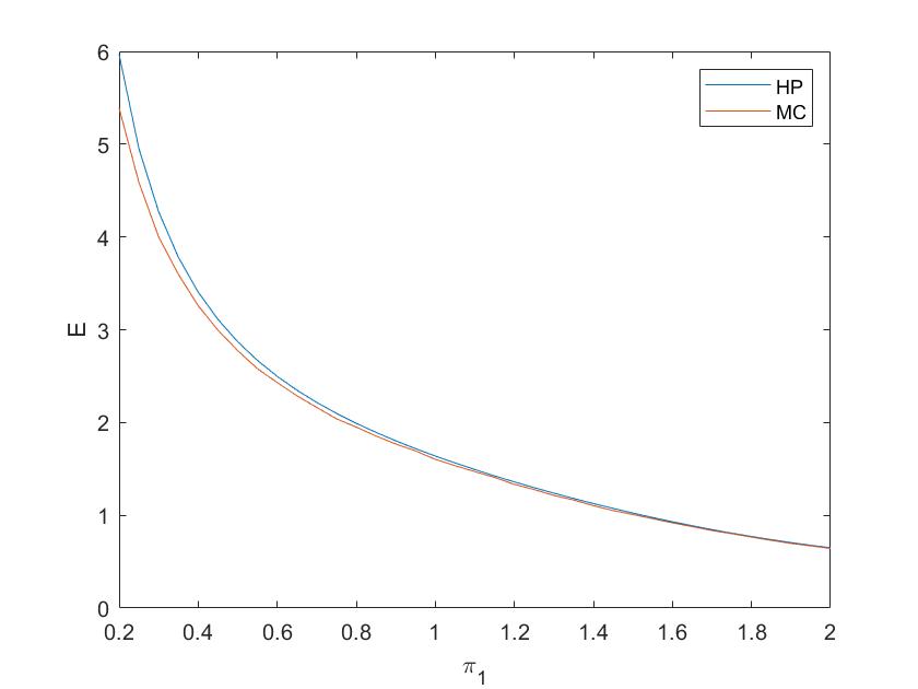
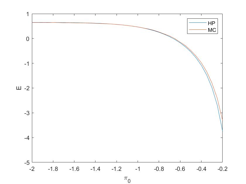
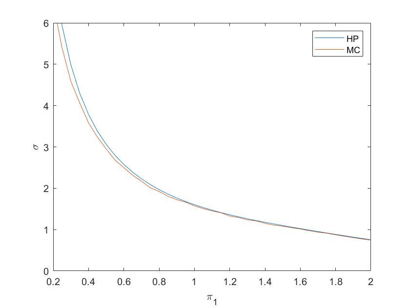
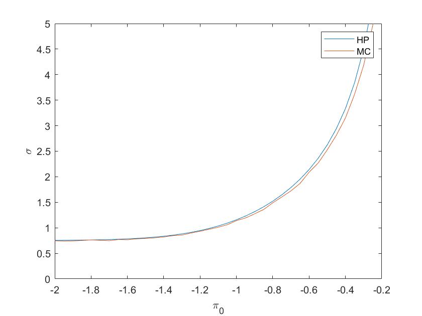
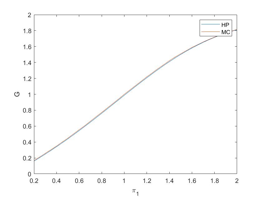
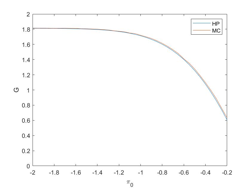
To be concrete, consider $\theta=1.0$ and $\Upsilon=0.49$, $T=1.96$. We compare our results with the Monte Carlo method, which simulates the process and compute its expectation and variance (see [35]). First, we compare separately $E$, $\sigma=\sqrt{F-E^{2}}$, and $G$ calculated by both methods in Figure 1:

Figure 1 near here.

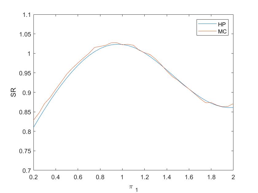
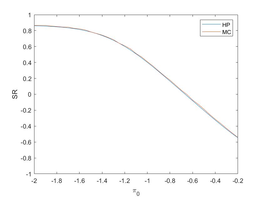
Second, we show the results for the $\operatorname{SR}$ itself in Figure 2:

Figure 2 near here.

We see that the relative difference between the method of heat potentials and the Monte Carlo method is small and mainly comes from the Monte Carlo noise.

7.2 Optimization of the Sharpe ratio

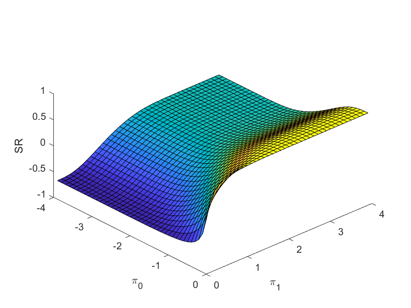
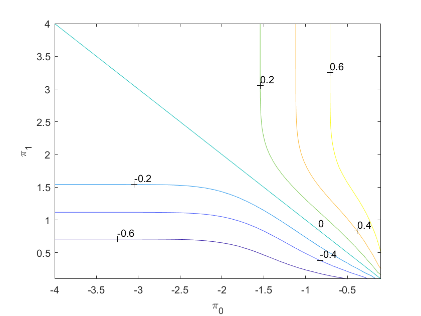
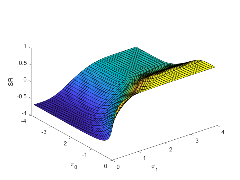
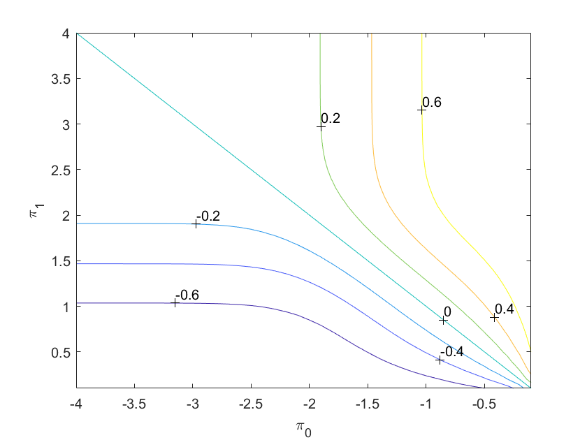
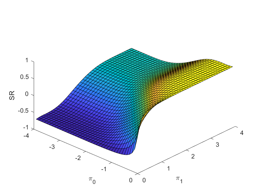
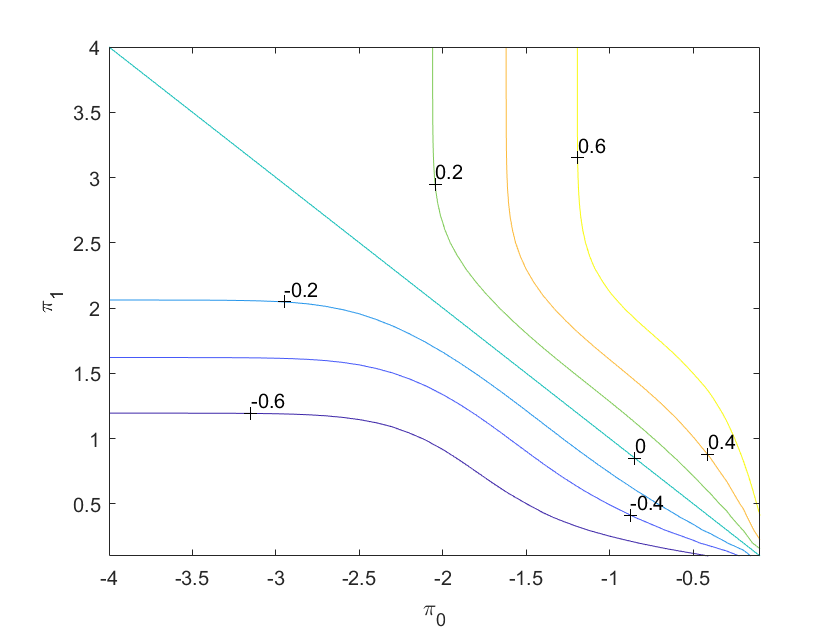
In this section we solve a problem of finding parameters to maximize the $\operatorname{SR}$ by analyzing it as a function of $(\underline{\pi},\overline{\pi})$ for different values of $\theta$ and $\Upsilon$. Two problems are considered: (A) Fix $\Upsilon$ and maximize the $\operatorname{SR}$ over $(\underline{\pi},\overline{\pi})$; (B) Maximize the $\operatorname{SR}$ over $(\underline{\pi},\overline{\pi},\Upsilon)$.

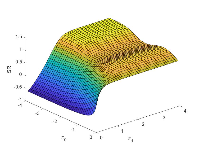
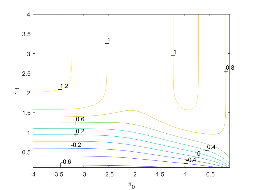
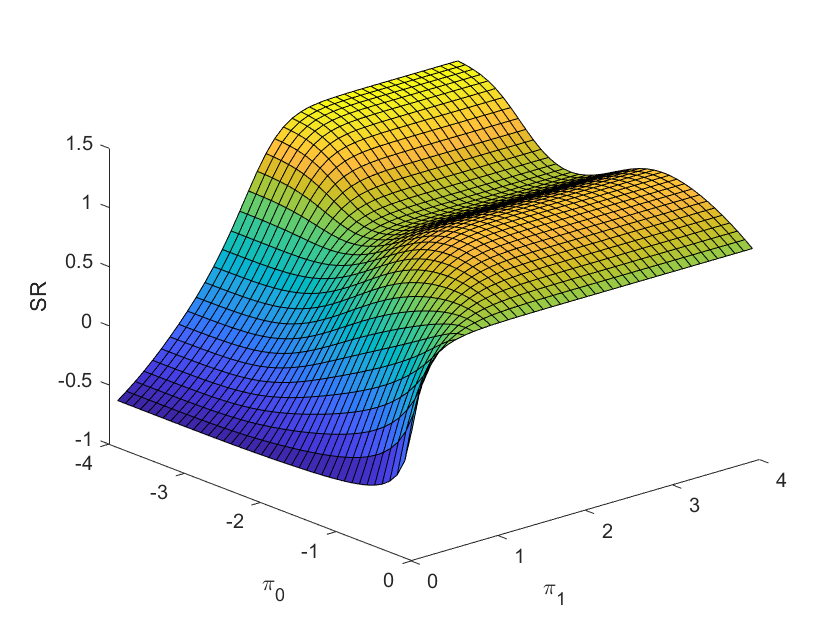
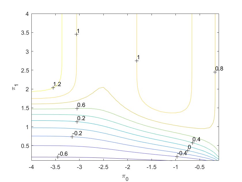
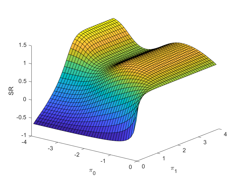
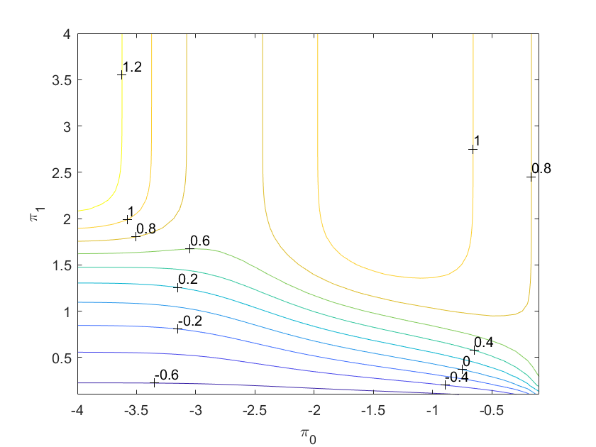
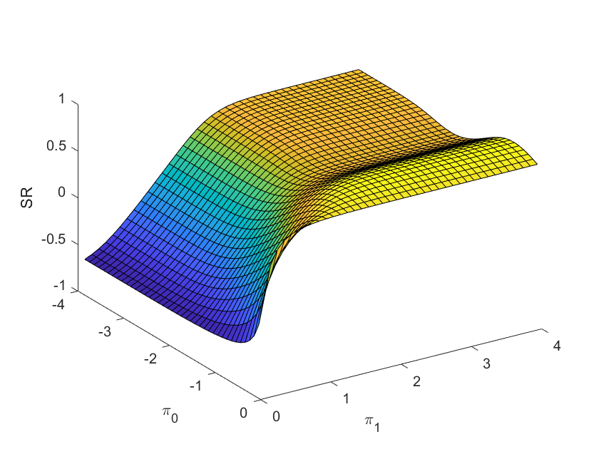
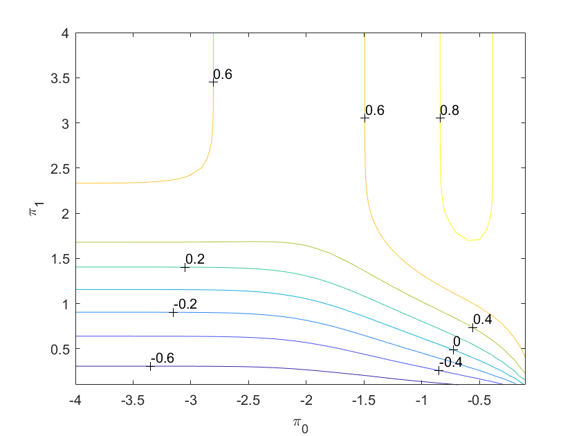
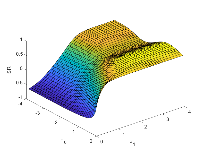
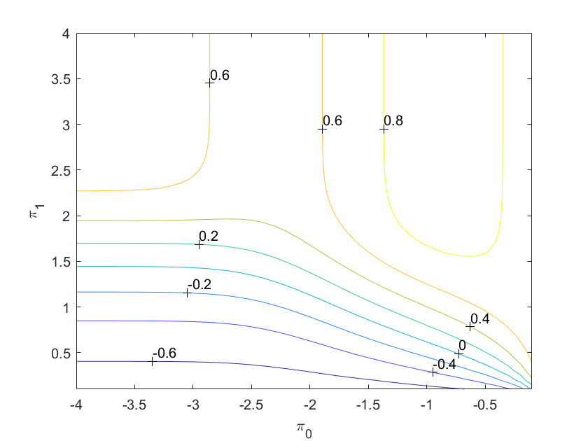
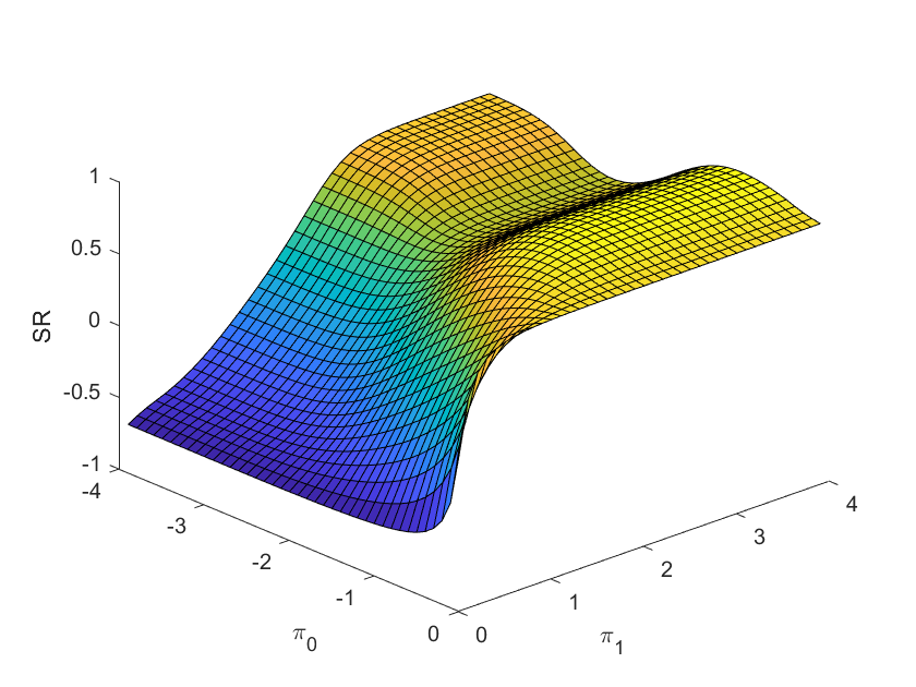
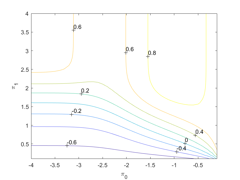
Given that the natural unit $\Omega=1/\sqrt{2}$, we consider three representative values of $\theta$, namely $\theta=1$, $\theta=0.5$, and $\theta=0$, corresponding to strong and weak mispricing and fair pricing, respectively. We choose three maturities, $\Upsilon=0.49$, $0.4999$, $0.499999$ or ,equivalently, $T=1.96$, $4.26$, $6.56$. For negative $\theta$, the corresponding $\operatorname{SR}$ can be obtained by reflection if needed.

We show the corresponding $\operatorname{SR}$ surfaces in Figures 3, 4, 5:

Figure 3 near here.

Figure 4 near here.

Figure 5 near here.

The optimal bounds $(\underline{\pi}^{\ast},\overline{\pi}^{\ast})$ are given in the Table 1 below:

Table 1 near here.

This table shows that in the case when the original mispricing is strong ($\theta=1$) it is not optimal to stop the trade early. When the mispricing is weaker ($\theta=0.5$) or there is no mispricing in the first place ($\theta=0$) it is not optimal to stop losses, but it might be beneficial to take profits. We emphasize that in practice one needs to use a highly reliable estimation of the O-U parameters to be able to use these rules with confidence.

8 Traditional approaches

8.1 Motivation

The method of heat potentials boils down to solving a system of Volterra equations of the second kind. However, there are certain quantities of interest, which can be calculated directly. To put it into a proper context, in this section we discuss several classical approached to the problem we are interested in. We emphasize that the method of heat potentials is dramatically different from other method because it allows one to consider strategies with finite duration, say $T$, whilst, to the best of our knowledge, all other methods are asymptotic in nature and assume that $T\rightarrow\infty$.

8.2 Expectation and variance of the trade’s duration

In this subsection, we calculate the expected value and the variance of the of duration of a trade, which terminates only when the spread hits one of the barriers, $T=\infty$ (or $\Upsilon=0.5$). Specifically, we show how to calculate these quantities analytically by solving inhomogeneous linear ordinary differential equations (ODEs).

In the case in question, the second change of variables is not necessary, so that we can concentrate on the following problems:

$$\begin{array}[]{c}G_{t}^{\left(1\right)}\left(t,x\right)+\left(\theta-x\right)G_{x}^{\left(1\right)}\left(t,x\right)+\frac{1}{2}G_{xx}^{\left(1\right)}\left(t,x\right)=0,\\ \\ G^{\left(2\right)}\left(t,\underline{\pi}\right)=t,\ \ \ G^{\left(1\right)}\left(t,\overline{\pi}\right)=t,\end{array}$$ (11)

$$\begin{array}[]{c}G_{t}^{\left(2\right)}\left(t,x\right)+\left(\theta-x\right)G_{x}^{\left(2\right)}\left(t,x\right)+\frac{1}{2}G_{xx}^{\left(2\right)}\left(t,x\right)=0,\\ \\ G^{\left(2\right)}\left(t,\underline{\pi}\right)=t^{2},\ \ \ G^{\left(2\right)}\left(t,\overline{\pi}\right)=t^{2}.\end{array}$$ (12)

with implicit terminal conditions at $T\rightarrow\infty$. The superscripts indicate the first and second moments, respectively.

We start with the expectation. We can represent the solution $G^{\left(1\right)}\left(t,x\right)$ of Eq. (11) in a semi-stationary form:

$$\begin{array}[]{c}G^{\left(1\right)}\left(t,x\right)=t+g^{\left(1\right)}\left(x\right),\end{array}$$

where

$$\begin{array}[]{c}\left(\theta-x\right)g_{x}^{\left(1\right)}\left(x\right)+\frac{1}{2}g_{xx}^{\left(1\right)}\left(x\right)=-1,\end{array}$$ (13)

$$\begin{array}[]{c}\ g^{\left(1\right)}\left(\underline{\pi}\right)=0,\ \ \ \ g^{\left(1\right)}\left(\overline{\pi}\right)=0.\end{array}$$ (14)

Eq. (13) can be solved by the method of variation of constants:

$$\begin{array}[]{c}g_{x}^{\left(1\right)}\left(x\right)=a_{1}e^{\left(x-\theta\right)^{2}}+\lambda\mathcal{F}\left(x-\theta\right),\\ \\ g^{\left(1\right)}\left(x\right)=a_{0}+a_{1}\mathcal{I}\left(x-\theta\right)+\lambda\mathcal{G}\left(x-\theta\right),\end{array}$$ (15)

where $a_{0}$, $a_{1}$ are arbitrary constants. Here $\mathcal{D}\left(x\right)$ is Dawson’s function, $\mathcal{E}\left(x\right)$ is its integral, and $\mathcal{F}\left(x\right),\mathcal{G}\left(x\right)$ are convenient abbreviations:

$$\begin{array}[]{c}\mathcal{I}\left(x\right)=\int_{0}^{x}e^{z^{2}}dz,\ \ \ \mathcal{D}\left(x\right)=e^{-x^{2}}\int_{0}^{x}e^{z^{2}}dz=e^{-x^{2}}\mathcal{I}\left(x\right),\\ \\ \mathcal{E}\left(x\right)=\int_{0}^{x}D\left(z\right)dz,\ \ \ \mathcal{F}\left(x\right)=\sqrt{\pi}N\left(\sqrt{2}x\right)e^{x^{2}},\\ \\ \mathcal{G}\left(x\right)=\sqrt{\pi}N\left(\sqrt{2}x\right)\mathcal{I}\left(x\right)-\mathcal{E}\left(x\right).\end{array}$$

We can use the Taylor series expansion for $\mathcal{G}\left(x\right)$ and represent it in the form

$$\begin{array}[]{c}\mathcal{G}\left(x\right)=\frac{1}{4}\mathop{\displaystyle\sum}\limits_{n=1}^{\infty}\frac{\Gamma\left(\frac{n}{2}\right)}{\Gamma\left(n+1\right)}\left(2x\right)^{n},\end{array}$$ (16)

see also [38], where this formula is obtained via the Laplace transform. Taking into account boundary conditions (14), we can represent $g$ as follows:

$$\begin{array}[]{c}g^{\left(1\right)}\left(x,\underline{\pi},\overline{\pi}\right)=2\left(\frac{\left(\mathcal{G}\left(\overline{\pi}-\theta\right)-\mathcal{G}\left(\underline{\pi}-\theta\right)\right)}{\left(\mathcal{I}\left(\overline{\pi}-\theta\right)-\mathcal{I}\left(\underline{\pi}-\theta\right)\right)}\left(\mathcal{I}\left(x-\theta\right)-\mathcal{I}\left(\underline{\pi}-\theta\right)\right)-\left(\mathcal{G}\left(x-\theta\right)-\mathcal{G}\left(\underline{\pi}-\theta\right)\right)\right).\end{array}$$ (17)

Finally, the expected duration is given by the following expression:

$$\begin{array}[]{c}\operatorname{DUR}=g\left(0\right).\end{array}$$ (18)

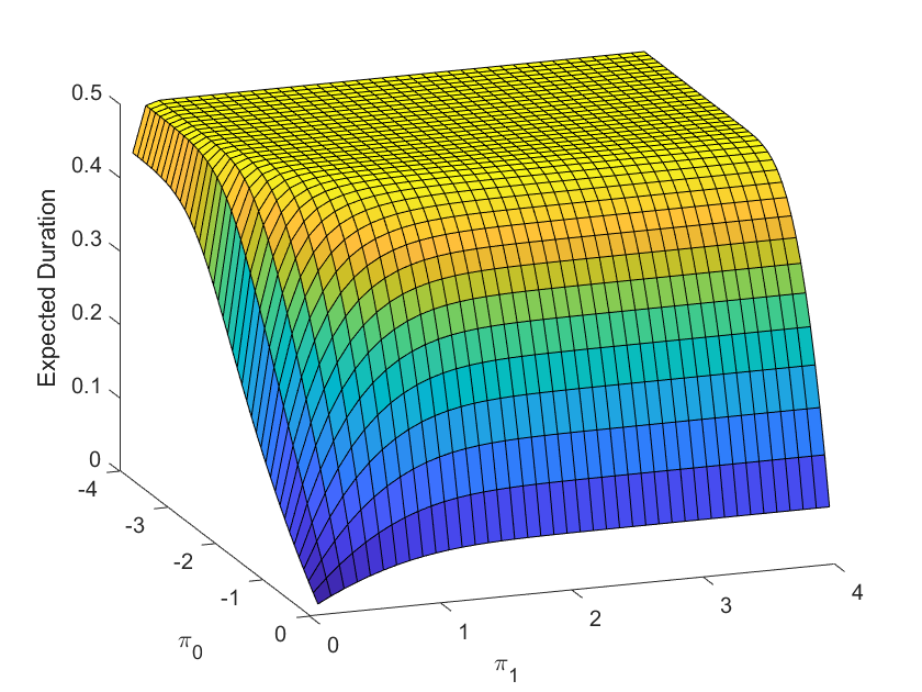
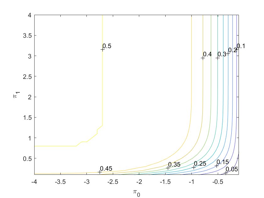
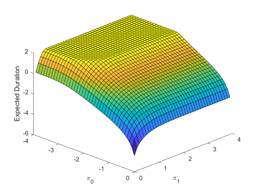
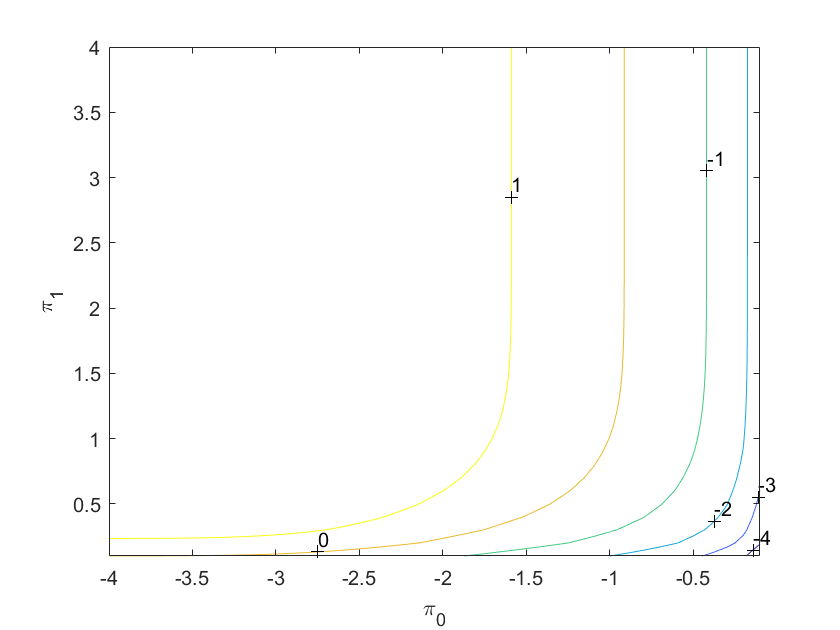
We show the expected duration as a function of $\underline{\pi},\overline{\pi}$ for $\theta=1$ in Figure 6:

Figure 6 near here.

Given the fact that $\Upsilon\rightarrow 0.5$ corresponds to $T\rightarrow\infty$, we can see from this Figure that for sufficiently remote $\underline{\pi},\overline{\pi}$ the process stays within the range $\left[\underline{\pi},\overline{\pi}\right]$ indefinitely, or, at least, for a very long time.

Now we consider Eq. (12) and write

$$\begin{array}[]{c}G^{\left(2\right)}\left(t,x\right)=t^{2}+tg^{\left(2,1\right)}\left(x\right)+g^{\left(2,0\right)}\left(x\right),\end{array}$$

where

$$\begin{array}[]{c}\left(\theta-x\right)g_{x}^{\left(2,1\right)}\left(x\right)+\frac{1}{2}g_{xx}^{\left(2,1\right)}\left(x\right)=-2,\\ \\ g^{\left(2,1\right)}\left(\underline{\pi}\right)=0,\ \ \ g^{\left(2,1\right)}\left(\overline{\pi}\right)=0,\end{array}$$

$$\begin{array}[]{c}\left(\theta-x\right)g_{x}^{\left(2,0\right)}\left(x\right)+\frac{1}{2}g_{xx}^{\left(2,0\right)}\left(x\right)=-g^{\left(2,1\right)}\left(x\right),\\ \\ g^{\left(2,0\right)}\left(\underline{\pi}\right)=0,\ \ \ g^{\left(2,0\right)}\left(\overline{\pi}\right)=0.\end{array}$$ (19)

In is clear that

$$\begin{array}[]{c}g^{\left(2,1\right)}\left(x\right)=2g^{\left(1\right)}\left(x,\underline{\pi},\overline{\pi}\right),\end{array}$$

where $g^{\left(1\right)}$ is given by Eq. (17).

Green’s function $\mathfrak{G}\left(x,y\right)$ for problem (19) has the form

$$\begin{array}[]{c}\mathfrak{G}\left(x,y\right)=\left\{\begin{array}[]{cc}2\frac{e^{-\left(y-\theta\right)^{2}}\left(\mathcal{I}\left(y-\theta\right)-\mathcal{I}\left(\underline{\pi}-\theta\right)\right)}{\left(\mathcal{I}\left(\overline{\pi}-\theta\right)-\mathcal{I}\left(\underline{\pi}-\theta\right)\right)}\left(\mathcal{I}\left(x-\theta\right)-\mathcal{I}\left(\overline{\pi}-\theta\right)\right)&y\leq x\leq\overline{\pi},\\ 2\frac{e^{-\left(y-\theta\right)^{2}}\left(\mathcal{I}\left(y-\theta\right)-\mathcal{I}\left(\overline{\pi}-\theta\right)\right)}{\left(\mathcal{I}\left(\overline{\pi}-\theta\right)-\mathcal{I}\left(\underline{\pi}-\theta\right)\right)}\left(\mathcal{I}\left(x-\theta\right)-\mathcal{I}\left(\underline{\pi}-\theta\right)\right)&\underline{\pi}\leq x\leq y.\end{array}\right.\end{array}$$

As usual,

$$\begin{array}[]{c}g^{\left(2,0\right)}\left(x\right)=-2\int_{-\infty}^{u}\mathfrak{G}\left(x,y\right)g^{\left(1\right)}\left(y,\underline{\pi},\overline{\pi}\right)dy.\end{array}$$

The explicit expression for the expected duration given by Eq. (18) is interesting in its own right and also can be used for benchmarking solutions obtained via the method of heat potentials.

8.3 Renewal theory approach

To facilitate the comparison with previously know results, from now on, we assume that $\theta=0$.

In this subsection, we revisit Bertram’s approach [6, 7]. In a nutshell, Bertram assumes that the underlying O-U process, representing portfolio’s log-price, is running in perpetuity. He envisions the following investment strategy. When the return process $x$ hits the lower level $l$, the underlying is bought. When the process $x$ hits the upper level $u$, the underlying is sold. Thus, the round trip is characterized by two transitions, $x=l\rightarrow x=u$, and $x=u\rightarrow x=l$; once the round trip is completed, the process starts again.

We can use the same ideas as in Section 8.2 to calculate $\mathbb{E}\left(T\right)$,$\mathbb{E}\left(T^{2}\right)$, and $\mathbb{V}\left(T\right)$ for the hitting time of a given level $u$, starting at the level $x=l$ by letting $\underline{\pi}\rightarrow-\infty,\overline{\pi}=u$:

$$\begin{array}[]{c}\mathbb{E}\left(T\right)=2\left(\mathcal{G}\left(u\right)-\mathcal{G}\left(l\right)\right),\\ \\ \mathbb{E}\left(T^{2}\right)=8\left(\mathcal{G}\left(u\right)\left(\mathcal{G}\left(u\right)-\mathcal{G}\left(l\right)\right)-\left(\mathcal{J}\left(u\right)-\mathcal{J}\left(l\right)\right)\right),\\ \\ \mathbb{V}\left(T\right)=4\left(\left(\mathcal{G}^{2}\left(u\right)-2\mathcal{J}\left(u\right)\right)-\left(\mathcal{G}^{2}\left(l\right)-2\mathcal{J}\left(l\right)\right)\right),\end{array}$$

where

$$\begin{array}[]{c}\mathcal{J}\left(x\right)=\int_{-\infty}^{x}e^{-y^{2}}\left(\mathcal{I}\left(x\right)-\mathcal{I}\left(y\right)\right)\mathcal{G}\left(y\right)dy\\ \\ =\mathcal{I}\left(x\right)\int_{-\infty}^{x}e^{-y^{2}}\mathcal{G}\left(y\right)dy-\int_{-\infty}^{x}\mathcal{D}\left(y\right)\mathcal{G}\left(y\right)dy.\end{array}$$

Similarly to Eq. (16), we can write:

$$\begin{array}[]{c}\mathcal{J}\left(x\right)=\frac{1}{16}\mathop{\displaystyle\sum}\limits_{n=1}^{\infty}\frac{\Gamma\left(\frac{n}{2}\right)\left(\psi\left(\frac{n}{2}\right)+\gamma\right)}{\Gamma\left(n+1\right)}\left(2x\right)^{n},\end{array}$$

where $\psi$ is the digamma function and $\gamma$ is the Euler-Mascheroni constant, $\gamma=-\psi\left(1\right)$, see also [38], where this formula is obtained via the Laplace transform.

In summary,

$$\begin{array}[]{c}\varepsilon\left(l\rightarrow u\right)\equiv\mathbb{E}\left(T\right)=2\left(\mathcal{G}\left(u\right)-\mathcal{G}\left(l\right)\right),\\ \\ \vartheta\left(l\rightarrow u\right)\equiv\mathbb{V}\left(T\right)=4\left(\left(\mathcal{G}^{2}\left(u\right)-2\mathcal{J}\left(u\right)\right)-\left(\mathcal{G}^{2}\left(l\right)-2\mathcal{J}\left(l\right)\right)\right).\end{array}$$

By symmetry,

$$\begin{array}[]{c}\varepsilon\left(u\rightarrow l\right)=\varepsilon\left(-u\rightarrow-l\right)=2\left(\mathcal{G}\left(-l\right)-\mathcal{G}\left(-u\right)\right),\\ \\ \vartheta\left(u\rightarrow l\right)=\vartheta\left(-u\rightarrow-l\right)=4\left(\left(\mathcal{G}^{2}\left(-l\right)-2\mathcal{J}\left(-l\right)\right)-\left(\mathcal{G}^{2}\left(-u\right)-2\mathcal{J}\left(-u\right)\right)\right).\end{array}$$

Finally,

$$\begin{array}[]{c}\varepsilon\left(l\rightarrow u\rightarrow l\right)\equiv\varepsilon\left(l\rightarrow u\right)+\varepsilon\left(u\rightarrow l\right)\\ \\ =2\left(\mathcal{G}\left(u\right)-\mathcal{G}\left(-u\right)-\left(\mathcal{G}\left(l\right)-\mathcal{G}\left(-l\right)\right)\right)\\ \\ =2\sqrt{\pi}\left(\mathcal{I}\left(u\right)-\mathcal{I}\left(l\right)\right),\end{array}$$

$$\begin{array}[]{c}\vartheta\left(l\rightarrow u\rightarrow l\right)\equiv\vartheta\left(l\rightarrow u\right)+\vartheta\left(u\rightarrow l\right)\\ \\ =4\left(\left(\mathcal{G}^{2}\left(u\right)-\mathcal{G}^{2}\left(-u\right)-2\left(\mathcal{J}\left(u\right)-\mathcal{J}\left(-u\right)\right)\right)-\left(\mathcal{G}^{2}\left(l\right)-\mathcal{G}^{2}\left(-l\right)-2\left(\mathcal{J}\left(l\right)-\mathcal{J}\left(-l\right)\right)\right)\right)\\ \\ =16\left(\left(\mathcal{G}^{\left(e\right)}\left(u\right)\mathcal{G}^{\left(o\right)}\left(u\right)-\mathcal{J}^{\left(o\right)}\left(u\right)\right)-\left(\mathcal{G}^{\left(e\right)}\left(l\right)\mathcal{G}^{\left(o\right)}\left(l\right)-\mathcal{J}^{\left(o\right)}\left(l\right)\right)\right)\end{array}$$

since $\mathcal{G}$, $\mathcal{J}$ are decomposed into the even and odd parts as follows:

$$\begin{array}[]{c}\mathcal{G}\left(x\right)=\mathcal{G}^{\left(e\right)}\left(x\right)+\mathcal{G}^{\left(o\right)}\left(x\right),\\ \\ \mathcal{G}^{\left(e\right)}\left(x\right)=\sqrt{\pi}\left(N\left(\sqrt{2}x\right)-\frac{1}{2}\right)\mathcal{I}\left(x\right)-\mathcal{E}\left(x\right),\\ \\ \mathcal{G}^{\left(o\right)}\left(x\right)=\frac{\sqrt{\pi}}{2}\mathcal{I}\left(x\right),\end{array}$$

$$\begin{array}[]{c}\mathcal{J}\left(x\right)=\mathcal{J}^{\left(e\right)}\left(x\right)+\mathcal{J}^{\left(o\right)}\left(x\right),\\ \\ \mathcal{J}^{\left(e\right)}\left(x\right)=\mathcal{I}\left(x\right)\int_{0}^{x}e^{-y^{2}}\mathcal{G}^{\left(e\right)}\left(y\right)dy-\int_{-\infty}^{0}\mathcal{D}\left(y\right)\mathcal{G}\left(y\right)dy-\int_{0}^{x}\mathcal{D}\left(y\right)\mathcal{G}^{\left(e\right)}\left(y\right)dy\\ \\ \mathcal{J}^{\left(o\right)}\left(x\right)=\mathcal{I}\left(x\right)\left(\int_{-\infty}^{0}e^{-y^{2}}\mathcal{G}\left(y\right)dy+\frac{\sqrt{\pi}}{2}\mathcal{E}\left(x\right)\right)-\frac{\sqrt{\pi}}{2}\int_{0}^{x}\mathcal{D}\left(y\right)\mathcal{I}\left(y\right)dy.\end{array}$$

Once the requisite quantities are computed, Bertram invokes classical results from renewal theory, [6, 7]. The classical result from renewal theory, see, e.g., [39], gives the asymptotic properties of the random variable $M\left(t,l,u\right)$ representing the number of round trips on the time interval $\left[0,t\right]$:

$$\begin{array}[]{c}M\left(t,l,u\right)\sim\mathfrak{N}\left(\frac{t}{\varepsilon\left(l\rightarrow u\rightarrow l\right)},\frac{\vartheta\left(l\rightarrow u\rightarrow l\right)t}{\varepsilon\left(l\rightarrow u\rightarrow l\right)^{3}}\right),\end{array}$$

where $\mathfrak{N}$ is the normal variable. Given that $x$ represents the log-price of the underlying portfolio, the return and asymptotic Sharpe ratio $\operatorname{SR}$ per unit of time are given by

$$\begin{array}[]{c}r=\frac{\left(u-l-c\right)}{\varepsilon\left(l\rightarrow u\rightarrow l\right)},\\ \\ \operatorname{SR}=\sqrt{\frac{\varepsilon\left(l\rightarrow u\rightarrow l\right)}{\vartheta\left(l\rightarrow u\rightarrow l\right)}}\frac{\left(u-l-c-r_{f}\right)}{\left(u-l-c\right)},\end{array}$$

where $c$, $r_{f}$ represent transaction fees, and risk-free rate, respectively. Bertram maximizes one of these quantities over the stop-loss/take profit thresholds $\left(l,u\right)$.

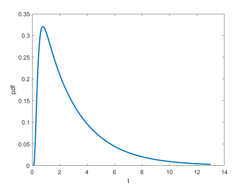
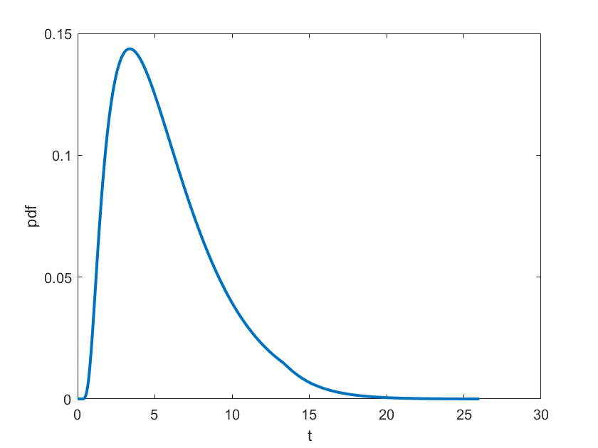
The main practical problem with this approach is that it assumes stationarity in perpetuity of the underlying process, which is a somewhat questionable assumption. The other problem is that, even for a stationary process, it takes a very long time for the strategy to reach its asymptotic state. The reason why these issues have not been discussed earlier, is that it is very hard to calculate the probability density function (pdf) for the processes $l\rightarrow u$, $u\rightarrow l$, and the round-trip process $l\rightarrow u\rightarrow l$. Recently, Lipton and Kaushansky proposed a very efficient method for calculating the pdfs for the processes $l\rightarrow u$, $u\rightarrow l$, see [31, 32]; the the round-trip process $l\rightarrow u\rightarrow l$ can be analyzed by convolution. We show the corresponding pdfs for a representative choice of $l$, $u$, namely $l=-1/\sqrt{2}$, $u=1/\sqrt{2}$ in Figure 7. This figure clearly shows that a very long right tail characterizes the round-trip process $l\rightarrow u\rightarrow l$, so that the strategy might never reach its asymptotic limit in practice.

Figure 7 near here.

8.4 Perpetual value function

In this section, we discuss results obtained in [12, 11, 23, 29], and rederive and improve their findings in a concise semi-analytic fashion.

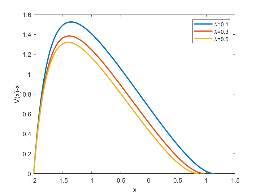
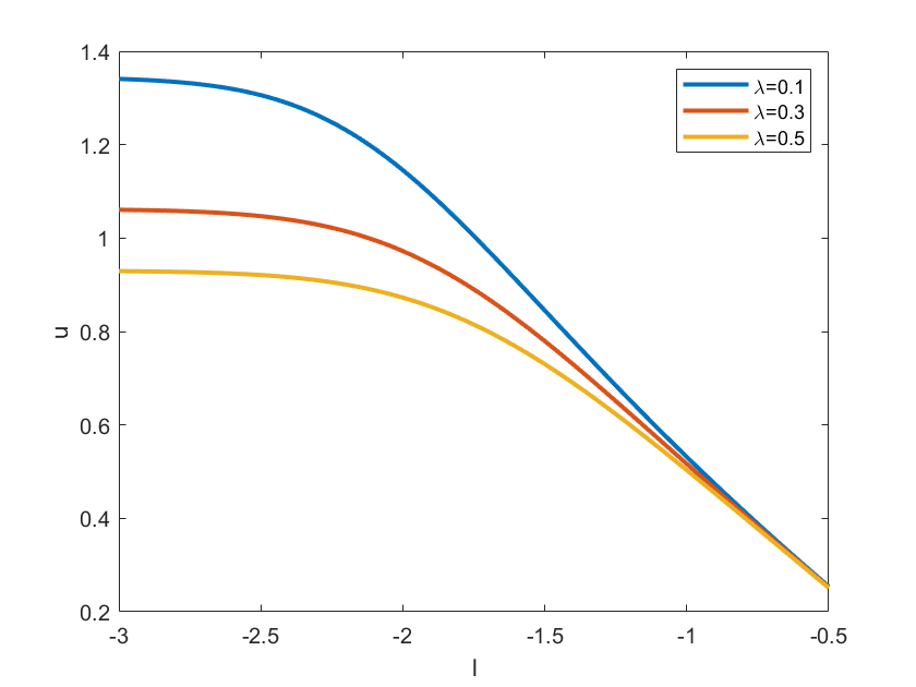
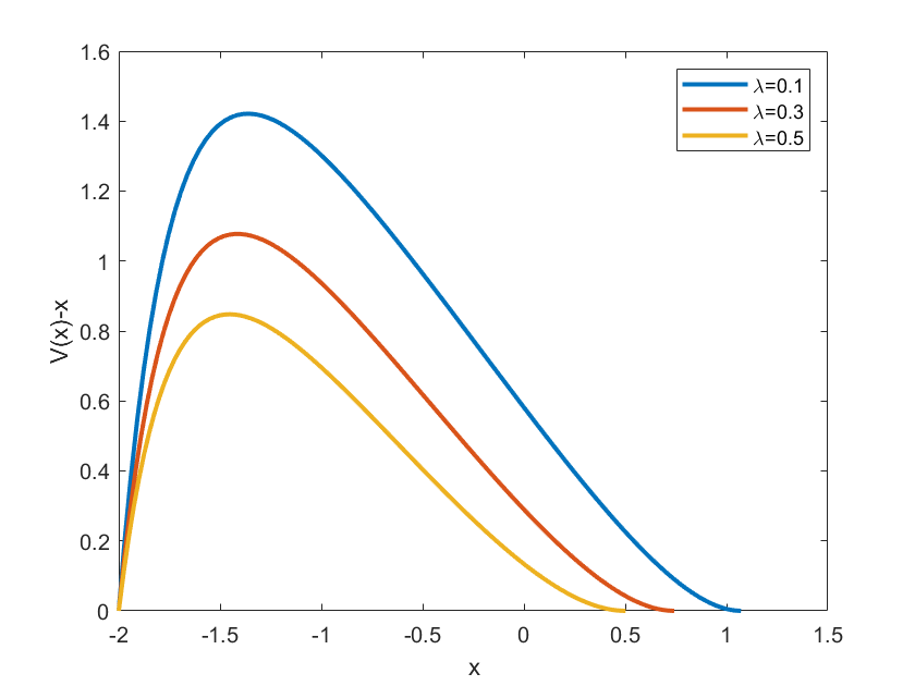
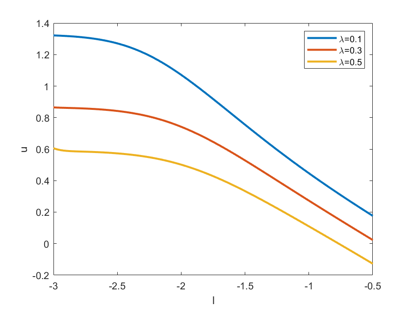
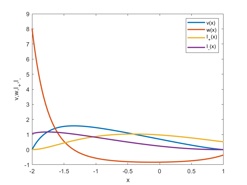
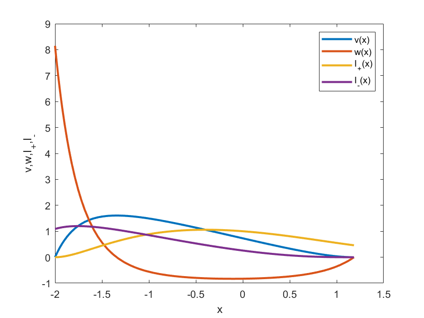
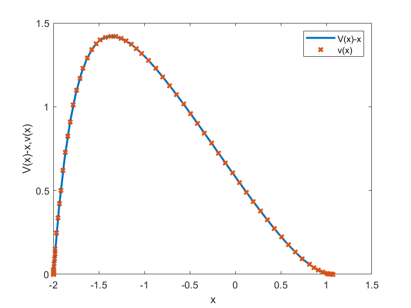
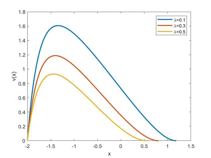
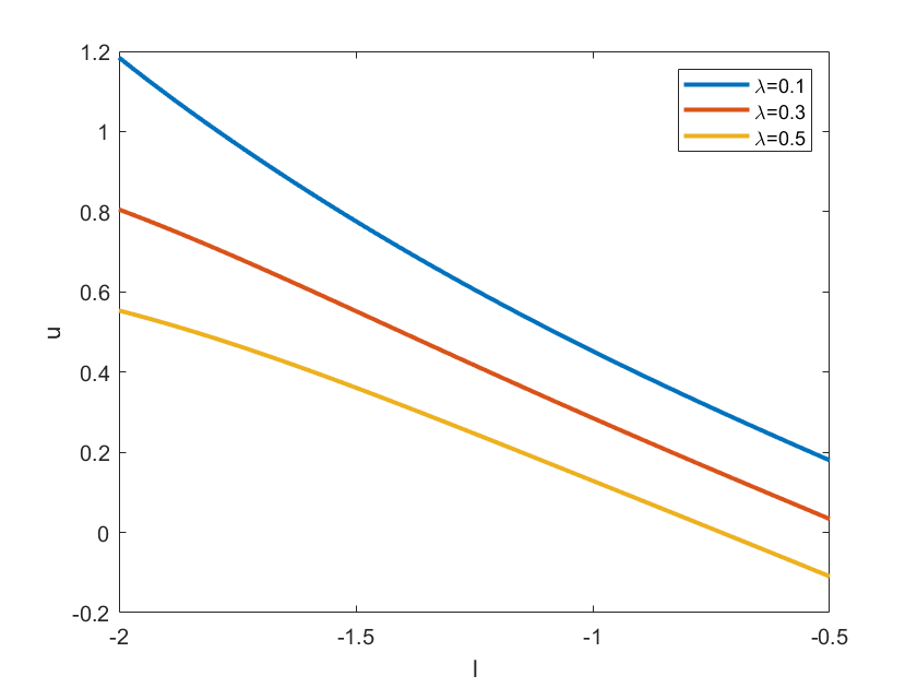
The stationary problem for determining the value function and the optimal take-profit level $u$ for a given stop-loss level $l$ (which is determined by the investor’s risk appetite) and the time value of money has the form:

$$\begin{array}[]{c}V_{xx}\left(x\right)-2xV_{x}\left(x\right)-\lambda V=0,\ \ \ l\leq x\leq u,\\ \\ V\left(l\right)=l,\ \ \ V\left(u\right)=u,\ \ \ V^{\prime}\left(u\right)=1.\end{array}$$ (20)

This problem is similar, but by no means identical, to the pricing problem for the perpetual American call option on a dividend-paying stock. Here $\lambda$ is the non-dimensional discount rate, $\lambda=2r/\kappa$.

The second-order ordinary differential equation (20) is the well-known Hermite differential equation. Its general solution has the form

$$\begin{array}[]{c}V\left(x\right)=a_{0}M\left(\frac{\lambda}{4},\frac{1}{2},x^{2}\right)+a_{1}xM\left(\frac{\lambda+2}{4},\frac{3}{2},x^{2}\right),\end{array}$$ (21)

where $M\left(a,b,z\right)$ is the celebrated Kummer function (a confluent hypergeometric function of the first kind), and $a_{0},a_{1}$ are arbitrary constants. Boundary conditions (20) yield:

$$\begin{array}[]{c}a_{0}M\left(\frac{\lambda}{4},\frac{1}{2},l^{2}\right)+a_{1}lM\left(\frac{\lambda+2}{4},\frac{3}{2},l^{2}\right)=l,\\ \\ a_{0}M\left(\frac{\lambda}{4},\frac{1}{2},u^{2}\right)+a_{1}uM\left(\frac{\lambda+2}{4},\frac{3}{2},u^{2}\right)=u,\\ \\ a_{0}\lambda uM\left(\frac{\lambda+4}{4},\frac{3}{2},u^{2}\right)+a_{1}\left(M\left(\frac{\lambda+2}{4},\frac{3}{2},u^{2}\right)+\frac{\left(\lambda+2\right)}{3}u^{2}M\left(\frac{\lambda+6}{4},\frac{5}{2},u^{2}\right)\right)=1.\end{array}$$

Here we use the fact that

$$\begin{array}[]{c}M_{z}\left(a,b,z\right)=\frac{a}{b}M\left(a+1,b+1,z\right).\end{array}$$

We eliminate $a_{0},a_{1}$:

$$\begin{array}[]{c}a_{0}=\frac{c_{11}l-c_{01}u}{c_{00}c_{11}-c_{01}c_{10}},\ \ \ a_{1}=\frac{-c_{10}l+c_{00}u}{c_{00}c_{11}-c_{01}c_{10}},\\ \\ c_{00}=M\left(\frac{\lambda}{4},\frac{1}{2},l^{2}\right),\ \ \ c_{01}=lM\left(\frac{\lambda+2}{4},\frac{3}{2},l^{2}\right),\\ \\ c_{10}=M\left(\frac{\lambda}{4},\frac{1}{2},u^{2}\right),\ \ \ c_{11}=uM\left(\frac{\lambda+2}{4},\frac{3}{2},u^{2}\right),\end{array}$$ (22)

and obtain the following nonlinear algebraic equation for $u$:

$$\begin{array}[]{c}\left(c_{11}l-c_{01}u\right)\lambda uM\left(\frac{\lambda+4}{4},\frac{3}{2},u^{2}\right)\\ \\ +\left(-c_{10}l+c_{00}u\right)\left(M\left(\frac{\lambda+2}{4},\frac{3}{2},u^{2}\right)+\frac{\left(\lambda+2\right)}{3}u^{2}M\left(\frac{\lambda+6}{4},\frac{5}{2},u^{2}\right)\right)=\left(c_{00}c_{11}-c_{01}c_{10}\right).\end{array}$$ (23)

We solve Eq. (23) via the Newton-Raphson method.

Once $u$ is found, we use Eqs (21), (22), to construct the value functions $V\left(x\right)$. We show $V\left(x\right)-x$ and $u\left(l\right)$ for several representative values of $\lambda$ in Figures 8 (a), (b).

Figure 8 near here.

The stationary problem for determining the value function and the optimal take-profit level $U$ for a given stop-loss level $L$ (which is determined by the investor’s risk appetite) and the opportunity cost $c$ has the nondimensional form:

$$\begin{array}[]{c}V_{xx}\left(x\right)-2xV_{x}\left(x\right)=\lambda,\ \ \ l\leq x\leq u,\\ \\ V\left(l\right)=l,\ \ \ V\left(u\right)=u,\ \ \ V_{x}\left(u\right)=1,\end{array}$$ (24)

where $\lambda$ is the non-dimensional opportunity cost, $\lambda=2c/\kappa$. It is easy to show that the general solution of Eq. (24) has the form given by Eq. (15). As before we get the following set of equations:

$$\begin{array}[]{c}a_{0}+a_{1}\mathcal{I}\left(l\right)=l-\lambda\mathcal{G}\left(l\right),\\ \\ a_{0}+a_{1}\mathcal{I}\left(u\right)=u-\lambda\mathcal{G}\left(u\right),\\ \\ a_{1}e^{u^{2}}=1-\lambda\mathcal{F}\left(u\right).\end{array}$$

Accordingly,

$$\begin{array}[]{c}a_{0}=\frac{\mathcal{I}\left(u\right)\left(l-\lambda\mathcal{G}\left(l\right)\right)-\mathcal{I}\left(l\right)\left(u-\lambda\mathcal{G}\left(u\right)\right)}{\left(\mathcal{I}\left(u\right)-\mathcal{I}\left(l\right)\right)},\\ \\ a_{1}=\frac{u-\lambda\mathcal{G}\left(u\right)-\left(l-\lambda\mathcal{G}\left(l\right)\right)}{\left(\mathcal{I}\left(u\right)-\mathcal{I}\left(l\right)\right)},\\ \\ \frac{e^{u^{2}}\left(u-\lambda\mathcal{G}\left(u\right)-\left(l-\lambda\mathcal{G}\left(l\right)\right)\right)}{\left(\mathcal{I}\left(u\right)-\mathcal{I}\left(l\right)\right)}=1-\lambda\mathcal{F}\left(u\right).\end{array}$$

In Figure 9(a), we show $V\left(x\right)-x$ for $l=-2.0$ for several representative values of $\lambda$, the corresponding optimal values of $u$ are $1.07$, $0.74$, $0.50$. In Figure 9(b) we show the optimal boundary $u\left(l\right)$.

Figure 9 near here.

It is natural to ask what happens when the underlying mean-reverting process has a jump component, so that

$$\begin{array}[]{c}dx=-xdt+dW_{t}+JdP_{t},\end{array}$$

where $P_{t}$ is a Poisson process with intensity $\nu$, and $J$ is the jump magnitude, which is assumed to be a random variable with density function $\phi\left(J\right)$, see [23]. Larsson et al. use the finite element method to solve the corresponding free boundary problem. However, if $J$ has a double exponential distribution density function $\phi\left(J\right)$,

$$\begin{array}[]{c}\phi\left(J\right)=\kappa e^{-\kappa\left|J\right|},\end{array}$$

or, more generally, a hyper-exponential distribution, see, e.g., [22], the problem can be solved in a semi-analytical fashion.

To this end, it is convenient to write the problem with jumps in terms of $v\left(x\right)=V\left(x\right)-x$:

$$\begin{array}[]{c}v^{\prime\prime}\left(x\right)-2xv^{\prime}\left(x\right)+\omega\left(I_{+}\left(x\right)+I_{-}\left(x\right)-v\left(x\right)\right)=\lambda+\left(2+\omega\right)x,\\ \\ I_{+}\left(x\right)=\mathop{\displaystyle\int}\limits_{0}^{x-l}v\left(x-z\right)e^{-\kappa z}dz=\mathop{\displaystyle\int}\limits_{l}^{x}v\left(z\right)e^{-\kappa\left(x-z\right)}dz,\\ \\ I_{-}\left(x\right)=\mathop{\displaystyle\int}\limits_{0}^{u-x}v\left(x+z\right)e^{-\kappa z}dz=\mathop{\displaystyle\int}\limits_{x}^{u}v\left(z\right)e^{-\kappa\left(z-x\right)}dz,\\ \\ v\left(l\right)=v\left(u\right)=v^{\prime}\left(u\right)=I_{+}\left(l\right)=I_{-}\left(u\right)=0,\end{array}$$

where $\omega=\kappa\nu$. It can be written as an inhomogeneous system of linear ODEs:

$$\begin{array}[]{c}v^{\prime}\left(x\right)-w\left(x\right)=0\\ \\ w^{\prime}\left(x\right)-2xw\left(x\right)+\omega\left(I_{+}\left(x\right)+I_{-}\left(x\right)-v\left(x\right)\right)=\lambda+\left(2+\omega\right)x,\\ \\ I_{+}^{\prime}\left(x\right)-v\left(x\right)+\kappa I_{+}\left(x\right)=0,\\ \\ I_{-}\left(x\right)+v\left(x\right)-\kappa I_{-}\left(x\right)=0,\\ \\ v\left(l\right)=0,\ \ \ w\left(l\right)=c,\ \ \ I_{+}\left(l\right)=0,\ \ \ I_{-}\left(l\right)=d.\end{array}$$

This system can be solved by the method of shooting by choosing initial values $c,d$ and the right endpoint of the computational interval $b$ to satisfy the remaining boundary conditions

$$\begin{array}[]{c}\ v\left(u\right)=w\left(u\right)=I_{-}\left(u\right)=0.\end{array}$$ (25)

or in the matrix form:

$$\begin{array}[]{c}\left(\begin{array}[]{c}v\\ w\\ I_{+}\\ I_{-}\end{array}\right)^{\prime}+\left(\begin{array}[]{cccc}0&-1&0&0\\ -\omega&-2x&\omega&\omega\\ -1&0&\kappa&0\\ 1&0&0&-\kappa\end{array}\right)\left(\begin{array}[]{c}v\\ w\\ I_{+}\\ I_{-}\end{array}\right)=\left(\begin{array}[]{c}0\\ \lambda+\left(2+\omega\right)x\\ 0\\ 0\end{array}\right).\end{array}$$

In Figure 10(a), we show the solution vector $\left(v\left(x\right),w\left(x\right),I_{+}\left(x\right),I_{-}\left(x\right)\right)$ corresponding to the suboptimal choice of $u$. The shooting parameters, $c,d$, are chosen in such a way, that two of the three boundary conditions (25) are satisfied, $v\left(u\right)=I_{-}\left(u\right)=0$. In Figure 10(b), we show what happens when the upper limit $u$ is chosen optimally, by using the Newton-Raphson method. For $u=1.18$ all three conditions (25) are met. In Figure 10(c), we demonstrate the quality of our numerical method by putting $\omega=0$ and comparing the corresponding numerical solution with the analytical solution given by Eq. (15). The figure shows that the agreement is excellent.

Figure 10 near here.

In Figure 11(a), we show $v\left(x\right)$ for $l=-2.0$, the corresponding optimal values of $u$ are $1.18$, $0.80$, $0.55$; we show $u\left(l\right)$ for several representative values of $\lambda$ in Figure 11(b), while

Figure 11 near here.

8.5 Linear transaction costs

Several researchers, including de Lataillade et al., [24], concentrated on the critical question on how linear transaction costs affect the profitability of mean-reverting trading strategies. An alternative treatment is given by [37], see also [9]. Denuded of all amenities, the approach of de Lataillade et al. is almost identical to the method used by Hyer et al., [19], for studying passport options.

de Lataillade et al. reduce the problem to solving the following Fredholm integral equation of the second kind

$$\begin{array}[]{c}g\left(x\right)-\int_{-q}^{q}K\left(x,y\right)g\left(y\right)dy=f\left(x\right),\end{array}$$ (26)

where

$$\begin{array}[]{c}K\left(x,y\right)=\frac{\Theta\exp\left(-\frac{\left(\Theta y-x\right)^{2}}{\left(\Theta^{2}-1\right)}\right)}{\sqrt{\pi\left(\Theta^{2}-1\right)}},\\ f\left(x\right)=x+\Gamma\left(N\left(-\frac{\sqrt{2}\left(\Theta q-x\right)}{\sqrt{\left(\Theta^{2}-1\right)}}\right)-N\left(-\frac{\sqrt{2}\left(\Theta q+x\right)}{\sqrt{\left(\Theta^{2}-1\right)}}\right)\right),\end{array}$$

where $\Theta=e^{\Delta}$. Eq. (26) is augmented with the matching condition

$$\begin{array}[]{c}g\left(q\right)=\Gamma.\end{array}$$ (27)

Here $\Gamma$ represents transaction cost, while $\Delta$ shows how far forward the behavior of the process can be predicted. The trader should not change her position when $-q<x<q$, and go maximally long when $x=q$, and short when $x=-q$.

While de Lataillade et al. use the path integral method to understand the behavior of Eqs (26,27), we prefer to attack the problem in question directly - by solving the corresponding Fredholm equation. As before, we solve Eq. (26) for a given $q$, and then adjust $q$ by using the Newton-Raphson method until the matching condition (27) is met. We notice in passing that $K\left(x,y\right)$ is even, $K\left(-x,-y\right)=K\left(x,y\right)$, while $f\left(x\right)$ is odd, $f\left(-x\right)=-f\left(x\right)$, so that $g\left(x\right)$ is even, $g\left(-x\right)=-g\left(x\right)$. Our analysis results in some unexpected findings. Namely, Eqs (26,27) have multiple solutions. We choose $\Gamma=0.1$, $\Delta=1$ and solve the equations in question. It turns out that at least two critical values of $q$ are possible, $q=0.0561$ and $q=1.0131$. We show the corresponding solutions in Figures 12(a), (b). It can be shown that $g\left(x\right)$, which has a single root at $x=0$ is the solution of interest. With this in mind, we can construct critical boundaries $q\left(\Delta\right)$ corresponding to several representative values of $\Gamma$. These boundaries are shown in Figure 12(c).

Figure 12 near here.

9 Conclusions

In this paper we create an analytical framework for computing optimal stop-loss/take-profit bounds $(\underline{\pi}^{\ast},\overline{\pi}^{\ast})$ for O-U driven trading strategies by using the method of heat potentials.

First, we present a method for calibrating the corresponding O-U process to market prices. Second, we derive an explicit expression for the $\operatorname{SR}$ given by Eq. (2), and maximize it with respect to the stop loss/ take profit bounds $(\underline{\pi},\overline{\pi})$. Third, for three representative values of $\theta$, we calculate the $\operatorname{SR}$ on a grid of $(\underline{\pi},\overline{\pi})$ and pre-chosen times and graphically summarize in Figures 3, 4, 5. Next, for each case, we perform optimization and present $(\underline{\pi}^{\ast},\overline{\pi}^{\ast})$ in Table 1. In agreement with intuition, in the case of strong misprising, it is optimal to wait until the trade’s expiration without imposing stop losses/ take profit bounds. For weaker mispricing, it is not optimal to stop losses, but it might be optimal to take profits early. Still, to be on the safe side, we recommend imposing stop losses chosen in accordance with one’s risk appetite to avoid unpleasant surprises caused by the misspecification of the underlying process.

Our rules help liquidity providers to decide how to offer liquidity to the market in the most profitable way, as well as by statistical arbitrage traders to optimally execute their trading strategies.

A very interesting and difficult multi-dimensional version of these rules (covering several correlated stocks) will be described elsewhere.

Acknowledgement 1

We greatly appreciate valuable discussions with Dr. Marsha Lipton, our partner at Investimizer.

Acknowledgement 2

We are grateful to Dr. Vadim Kaushansky for his help with an earlier version of this paper.

$\theta$ $\backslash$ $\Upsilon,T$	$0.49,\ 0.8$	$0.4999,\ 1.96$	$0.499999,\ 4.26$
$1.0$	$\underline{\pi}^{\ast}=-4.0$ $\overline{\pi}^{\ast}=4.0$ $\operatorname{SR}=1.2261$	$\underline{\pi}^{\ast}=-4.0$ $\overline{\pi}^{\ast}=4.0$ $\operatorname{SR}=1.3824$	$\underline{\pi}^{\ast}=-4.0$ $\overline{\pi}^{\ast}=4.0$ $\operatorname{SR}=1.3709$
$0.5$	$\underline{\pi}^{\ast}=-4.0$ $\overline{\pi}^{\ast}=0.6$ $\operatorname{SR}=0.8219$	$\underline{\pi}^{\ast}=-4.0$ $\overline{\pi}^{\ast}=0.9$ $\operatorname{SR}=0.8792$	$\underline{\pi}^{\ast}=-4.0$ $\overline{\pi}^{\ast}=1.0$ $\operatorname{SR}=0.8963$
$0.0$	$\underline{\pi}^{\ast}=-4.0$ $\overline{\pi}^{\ast}=0.1$ $\operatorname{SR}=0.7075$	$\underline{\pi}^{\ast}=-4.0$ $\overline{\pi}^{\ast}=0.4$ $\operatorname{SR}=0.7139$	$\underline{\pi}^{\ast}=-4.0$ $\overline{\pi}^{\ast}=0.1$ $\operatorname{SR}=0.7411$

Table 1: The Sharpe Ratio maximized over $(\underline{\pi},\overline{\pi})$ for fixed $\Upsilon$ or $T$.

(a)

(b)

(c)

(d)

(e)

(f)

Figure 1: (a) $E,\sigma=\sqrt{F-E^{2}}$ and $G$ as functions of $\overline{\pi}\equiv\pi_{1}$ computed by using the method of heat potentials and the Monte Carlo method for $\underline{\pi}=-2$; (b) Same quantities as functions of $\underline{\pi}\equiv\pi_{0}$ computed using the method of heat potentials and the Monte Carlo method for $\overline{\pi}=1$; $\theta=1.0$, $T=1.96$.

(a)

(b)

Figure 2: (a) The Sharpe ratio as a function of $\overline{\pi}\equiv\pi_{1}$ computed by using the method of heat potentials and the Monte Carlo method for $\underline{\pi}=-1$ (b) the Sharpe ratio as a function of $\underline{\pi}\equiv\pi_{0}$ computed using the method of heat potentials and the Monte Carlo method for $\overline{\pi}=1$; $\theta=1.0$, $T=1.96$.

(a)

(b)

(c)

(d)

(e)

(f)

Figure 3: The Sharpe Ratio as a function of $(\underline{\pi},\overline{\pi})$ for $\theta=1.0$ a)-b) $T=1.96$, c)-d) $T=4.26$, e)-f) $T=6.56$.

(a)

(b)

(c)

(d)

(e)

(f)

Figure 4: The Sharpe Ratio as a function of $(\underline{\pi},\overline{\pi})$ for $\theta=0.5$ a)-b) $T=1.96$, c)-d) $T=4.26$, e)-f) $T=6.56$.

(a)

(b)

(c)

(d)

(e)

(f)

Figure 5: The Sharpe Ratio as a function of $(\underline{\pi},\overline{\pi})$ for $\theta=0.0$ a)-b) $T=1.96$, c)-d) $T=4.26$, e)-f) $T=6.56$.

(a)

(b)

(c)

(d)

Figure 6: In Figures (a)-(b) we show the expected duration $\Upsilon=\left(1-\exp\left(-2G\right)/2\right)$ as a function of $\underline{\pi}$, $\overline{\pi}$; in Figures (c)-(d) we show the logarithm of the expected duration $G$. The corresponding $\theta=1.0$. Here and in Figures 3, 4, 5 $\pi_{0}\equiv\underline{\pi}$, $\pi_{1}\equiv\overline{\pi}$.

(a)

(b)

Figure 7: Figure (a) shows the pdf for the process $l\rightarrow u$; Figure (b) shows the pdf for the round-trip process $l\rightarrow u\rightarrow l$. The corresponding $l=-1/\sqrt{2}$, $u=1/\sqrt{2}$. We make this choice because one standard deviation of the stationary O-U distribution is $1/\sqrt{2}$.

(a)

(b)

Figure 8: Figure (a) shows the nondimensional value function $V\left(x\right)-x$ for several representative values of $\lambda$, the corresponding optimal values of $u$ are $1.15$, $0.97$, $0.87$; Figure (b) shows the nondimensional optimal take-profit boundary $u$ as a function of the nondimensional stop-loss boundary $l$.

(a)

(b)

Figure 9: Figure (a) shows the nondimensional value function $V\left(x\right)-x$ for $l=-2.0$, and several representative values of $\lambda$, the corresponding optimal values of $u$ are $1.07$, $0.74$, $0.50$; Figure (b) shows the nondimensional optimal execution boundary $u\left(l\right)$.

(a)

(b)

(c)

Figure 10: Figure (a) shows the nondimensional value functions $v\left(x\right)$ for $l=-2.0$, $\lambda=0.1$, $\omega=0.1$, $\kappa=1.0$. We choose $u=1$, which is not optimal. Hence, the matching condition is not satisfied. Figure (b) shows the value function $v\left(x\right)$ for the optimal value of $u=1.18$. Since $u$ is optimal, the matching condition is met, so that $w\left(u\right)=0$. Figure (c) shows the nondimensional value functions $v\left(x\right)$ for $l=-2.0$, $u=1.18$, $\lambda=0.1$, $\omega=0.0$, $\kappa=1.0$.

(a)

(b)

Figure 11: Figure (a) shows the nondimensional value functions $v\left(x\right)$ for $l=-2.0$, and several representative values of $\lambda$, the corresponding optimal values of $u$ are $1.18$, $0.81$Figure (b) shows the nondimensional optimal execution boundary $u\left(l\right)$. Here $\omega=0.1$, $\kappa=1.0$.

(a)

(b)

(c)

Figure 12: In Figure (a) we show $g\left(x\right)$ corresponding to the critical value $q=0.0561$; in Figure (b) we show $g\left(x\right)$ corresponding to the critical value $q=1.0131$. We can see that in the fist case $g\left(x\right)$ has a single root at $x=0$, while in the second case, there are three roots. In Figure (c) we show critical boundaries $q\left(\Delta\right)$ corresponding to three representative values of $\Gamma$, $\Gamma=0.05$, $0.10$, $0.20$. It is clear that for larger values of $\Gamma$, it is beneficial to wait longer before changing one’s position.

References

• [1] Avellaneda, M. and Lee, J.-H., 2010. Statistical arbitrage in the us equities market. Quantitative Finance, 10(7):761-782.
• [2] Bai, Y., Wu, L., 2018. Analytic value function for optimal regime-switching pairs trading rules. Quantitative Finance 18 (4), 637-654.
• [3] Bailey D. H. and Lopez De Prado, M., 2013. The Sharpe Ratio Efficient Frontier. Journal of Risk, 15(2).
• [4] Bailey D. H. and Lopez De Prado, M., 2014. The Deflated Sharpe Ratio: Correcting for Selection Bias, Backtest Overfitting and Non-Normality. Journal of Portfolio Management, 40(5):94-107.
• [5] Baviera, R., Baldi, T. S., 2017. Stop-loss and leverage in optimal statistical arbitrage with an application to energy market. Working paper, Politecnico di Milano.
• [6] Bertram, W.K., 2009. Optimal trading strategies for Ito diffusion processes. Physica A: Statistical Mechanics and its Applications, 388(14): 2865-2873.
• [7] Bertram, W.K., 2010. Analytic solutions for optimal statistical arbitrage trading. Physica A: Statistical Mechanics and its Applications, 389(11): 2234-2243.
• [8] Cummins, M., Bucca, A., 2012. Quantitative spread trading on crude oil and refined products markets. Quantitative Finance 12 (12): 1857-1875.
• [9] Do, B., Faff, R., 2012. Are pairs trading profits robust to trading costs? Journal of Financial Research 35 (2), 261-287.
• [10] Endres, S., Stübinger, J., 2017. Optimal trading strategies for Lévy-driven Ornstein-Uhlenbeck processes. FAU Discussion Papers in Economics, No. 17/2017, Friedrich-Alexander-Universität Erlangen-Nürnberg.
• [11] Ekstrom, E., Lindberg, C., Tysk, J., 2011. Optimal liquidation of a pairs trade. In: Di Nunno, G., Oksendal, B. (Eds.), Advanced mathematical methods for finance. Springer, Berlin, Heidelberg, pp. 247-255.
• [12] Ekstrom, E., Lindberg, C., Tysk, J., Wanntorp, H., 2010. Optimal liquidation of a call spread. Journal of Applied Probability 47, 586-593.
• [13] Elliott, R. J., Van Der Hoek, J., and Malcolm, W. P. (2005). Pairs trading. Quantitative Finance, 5(3):271-276.
• [14] Gatev, E., Goetzmann, W. N., Rouwenhorst, K. G., 2006. Pairs trading: Performance of a relative-value arbitrage rule. Review of Financial Studies 19 (3), 797-827.
• [15] Govender, K., 2011. Statistical arbitrage in South African financial markets. Working paper, University of Cape Town.
• [16] Goncu, A., Akyldirim, E., 2016. Statistical arbitrage with pairs trading. International Review of Finance 16 (2), 307-319.
• [17] Gregory, I., Ewald, C.-O., Knox, P., 2011. Analytical pairs trading under different assumptions on the spread and ratio dynamics. Working paper, University of Sydney.
• [18] Huck, N., Afawubo, K., 2015. Pairs trading and selection methods: Is cointegration superior? Applied Economics 47 (6), 599-613.
• [19] Hyer T., Lipton-Lifschitz, A., Pugachevsky D., 1997. Passport to success. Risk Magazine 10(9), 127-131.
• [20] Kartashov, E., 2001. Analytical Methods in the Theory of Heat Conduction of Solids. Vysshaya Shkola, Moscow 706.
• [21] Krauss, C., 2015. Statistical arbitrage pairs trading strategies: Review and outlook, IWQW Discussion Papers, No. 09/2015, Friedrich-Alexander-Universität Erlangen-Nürnberg.
• [22] Lipton, A., 2002. Assets with jumps. Risk Magazine 15 (9), 149-153.
• [23] Larsson, S., Lindberg, C., Warfheimer, M., 2013. Optimal closing of a pair trade with a model containing jumps. Applications of Mathematics 58 (3), 249-268.
• [24] de Lataillade, J., Deremble, C., Potters, M., Bouchaud, J-P. 2012. Optimal trading with linear costs. Journal of Investment Strategies 1(3): 91-115.
• [25] Leung, T., Li, X., 2015a. Optimal mean reversion trading: Mathematical analysis and practical applications. World Scientific, New Jersey, USA.
• [26] Leung, T., Li, X., 2015b. Optimal mean reversion trading with transaction costs and stop-loss exit. International Journal of Theoretical and Applied Finance 18 (3), 1550020.
• [27] Li, X., 2015. Optimal multiple stopping approach to mean reversion trading. PhD thesis, Columbia University.
• [28] Liu, B., Chang, L.-B., Geman, H., 2017. Intraday pairs trading strategies on high frequency data: The case of oil companies. Quantitative Finance 17 (1), 87-100.
• [29] Lindberg, C., 2014. Pairs trading with opportunity cost. Journal of Applied Probability 51, 282-286.
• [30] Lipton, A., 2001. Mathematical Methods for Foreign Exchange: A Financial Engineer’s Approach. World Scientific, Singapore.
• [31] Lipton, A. and Kaushansky, V., 2018. On the first hitting time density of an Ornstein-Uhlenbeck process. arXiv preprint arXiv:1810.02390.
• [32] Lipton, A. and Kaushansky, V., 2020. On the first hitting time density for a reducible diffusion process. Quantitative Finance, , DOI: 10.1080/14697688.2020.1713394.
• [33] Lipton, A. and Kaushansky, V., 2020. Physics and Derivatives: On Three Important Problems in Mathematical Finance. The Journal of Derivatives.
• [34] Lipton, A., Kaushansky, V. and Reisinger, C., 2019. Semi-analytical solution of a McKean–Vlasov equation with feedback through hitting a boundary. European Journal of Applied Mathematics, DOI: 10.1017/S0956792519000342.
• [35] Lopez De Prado, M., 2018. Advances in financial machine learning. John Wiley & Sons, Hoboken, NJ, USA.
• [36] Lopez De Prado, M., 2019. Tactical Investment Algorithms. https://ssrn.com/abstract=3459866.
• [37] Martin, R., Schöneborn, T., 2011. Mean reversion pays, but costs. Risk Magazine 24(2), 96-101.
• [38] Ricciardi, L.M., Sato, S., 1988. First-passage-time density and moments of the Ornstein–Uhlenbeck process. Journal of Applied Probability 25(1), 43–57.
• [39] Ross, S.M., 2010. Introduction to Probability Models. Tenth Edition. Academic Press, San Diego, CA, USA
• [40] Rubinstein, L. 1971. The Stefan Problem. Vol. 27 of Translations of Mathematical Monographs. American Mathematical Society, Providence, RI.
• [41] Suzuki, K., 2018. Optimal pair-trading strategy over long/short/square positions|||empirical study. Quantitative Finance 18 (1), 97-119.
• [42] Tikhonov, A. N., Samarskii, A.A., 1963. Equations of Mathematical Physics. Dover Publications, New York. English translation.
• [43] Vidyamurthy, G., 2004. Pairs trading: Quantitative methods and analysis. John Wiley & Sons, Hoboken, NY, USA.
• [44] Watson, N.A., 2012. Introduction to Heat Potential Theory. Number 182 in Mathematical Surveys and Monographs. American Mathematical Society, Providence, RI.
• [45] Zeng, Z., Lee, C.-G., 2014. Pairs trading: Optimal thresholds and profitability. Quantitative Finance 14 (11), 1881-1893.
θ𝜃\theta \\\backslash Υ,TΥ𝑇\Upsilon,T 0.49, 0.80.490.80.49,\ 0.8 0.4999, 1.960.49991.960.4999,\ 1.96 0.499999, 4.260.4999994.260.499999,\ 4.26
1.01.01.0
π¯=4.0superscript¯𝜋4.0\underline{\pi}^{\ast}=-4.0
π¯=4.0superscript¯𝜋4.0\overline{\pi}^{\ast}=4.0
SR=1.2261SR1.2261\operatorname{SR}=1.2261
SR=1.3824SR1.3824\operatorname{SR}=1.3824
SR=1.3709SR1.3709\operatorname{SR}=1.3709
0.50.50.5
π¯=0.6superscript¯𝜋0.6\overline{\pi}^{\ast}=0.6
SR=0.8219SR0.8219\operatorname{SR}=0.8219
π¯=0.9superscript¯𝜋0.9\overline{\pi}^{\ast}=0.9
SR=0.8792SR0.8792\operatorname{SR}=0.8792
π¯=1.0superscript¯𝜋1.0\overline{\pi}^{\ast}=1.0
SR=0.8963SR0.8963\operatorname{SR}=0.8963
0.00.00.0
π¯=0.1superscript¯𝜋0.1\overline{\pi}^{\ast}=0.1
SR=0.7075SR0.7075\operatorname{SR}=0.7075
π¯=0.4superscript¯𝜋0.4\overline{\pi}^{\ast}=0.4
SR=0.7139SR0.7139\operatorname{SR}=0.7139
SR=0.7411SR0.7411\operatorname{SR}=0.7411